

Submitted:
27 May 2026
Posted:
28 May 2026
You are already at the latest version
Abstract
Transforming energy supply systems is vital for achieving a sustainable, carbon-neutral future. However, this transformation entails significant complexity, driven by the integration of carbon-free energy sources, tightly coupled technical and economic subsystems, and the need to ensure reliability, resilience, and affordability. Addressing these challenges requires advanced planning approaches capable of capturing uncertainty, multiple stakeholder perspectives, and system dynamics across temporal and spatial scales. In response, this article presents an integrated planning and operational framework that combines multi-actor, multi-criteria, and multi-stage stochastic optimization with surrogate modelling and artificial intelligence. The proposed approach enhances scalability, computational efficiency, and precision in the planning and operation of future energy systems. A case study illustrates its effectiveness in supporting high-resolution, uncertainty-aware decision-making.
Keywords:
power system
; optimization
; planning
; electricity market
; artificial intelligence
; renewables
1. Introduction
1.1. Transforming Energy Supply
The widespread electrification, decentralized generation, and a heavy reliance on variable renewable energy sources (RES) such as solar and wind [1,2] introduces substantial complexity due to their inherent variability, limited dispatchability, and the consequent need for large-scale energy storage and flexible grid operation [3,4]. Ensuring reliability, operational flexibility, and long-term resilience in such a dynamic and uncertain environment requires advanced planning tools and robust decision support frameworks capable of addressing uncertainty, modeling complex interactions, and evaluating a vast space of technological and operational alternatives [5,6].
The inherent importance and complexity of energy supply sector have motivated a wide range of scholarly and practical efforts aimed at developing decision-support tools capable of facilitating rational and effective planning [7,8,9,10]. However, a review of the current scientific literature reveals that no universally accepted methodologies or tools have yet been developed to comprehensively address this multifaceted issue.
Among the principal challenges in large-scale energy planning are substantial computational complexities. A significant portion of the principal challenges in large-scale energy planning arises from the involvement of a diverse array of stakeholders – ranging from policymakers and utilities to investors, regulators, and end-users—each guided by distinct, and often conflicting, objectives, priorities, and decision-making criteria. This fragmentation can lead to suboptimal investment decisions, policy misalignment, and delayed implementation, ultimately undermining the efficiency and effectiveness of the energy transition [6].
The limited availability of computational resources significantly restricts the ability to conduct detailed analysis across a broad set of scenarios and alternatives. Scenarios in this context typically encompass diverse combinations of technological pathways, policy interventions, market dynamics, investment strategies, and demand evolution trajectories – each reflecting different assumptions about the future. Effective decision-making requires not only evaluating these scenarios individually, but also comparing them across multiple dimensions such as cost, emissions, reliability, and social acceptability. Moreover, different stakeholders may prioritize these criteria differently.
The vast number of plausible futures and the complexity of evaluating outcomes from multiple points of view make comprehensive scenario analysis computationally demanding. Consequently, planners are often forced to limit the number or granularity of scenarios considered, which can lead to oversimplified models and a loss of robustness, nuance, and reliability in the resulting strategies.
1.2. Power System Planning
The power system considered in this study is a large-scale, highly complex system composed of numerous interacting components and decision-makers operating across multiple time horizons. It comprises:
- dispatchable generation units, including thermal, nuclear, conventional reservoir hydropower, and pumped-storage hydropower facilities;
- variable renewable energy sources, such as solar, wind, and run-of-river hydropower;
- energy storage technologies, encompassing both short-duration and long-duration storage systems;
- the electrical transmission and distribution infrastructure;
- end-users, including both consumers and prosumers;
- institutional and market entities, including governmental authorities, Transmission System Operators (TSOs), and the market operator.
System behavior is influenced by decisions taken at both short- and long-term horizons, which differ fundamentally in their objectives and control variables. Short-term operational planning [11] focuses on the selection of energy volumes generated or consumed over short time intervals (e.g., hourly or daily), with the objective of maximizing operational profitability subject to technical and market constraints. In practice, short-term planning is typically carried out on an hourly or sub-hourly basis and is frequently coordinated through market-based mechanisms, including—but not limited to—the day-ahead electricity market. Within these frameworks, market participants submit bids and offers at the relevant time resolution, and market-clearing prices and traded volumes are determined through the interaction of supply and demand [12]. Such planning is performed for a given system configuration and installed generation capacities and does not involve investment decisions or structural modifications of the energy system.
In contrast, long-term planning decisions determine the structural evolution of the power system and involve the selection of generation technologies, installed capacities of generation and storage units, grid infrastructure elements, and, in some cases, the scale and characteristics of demand-side resources. These decisions do not directly determine short-term operational variables; rather, they define the feasible space within which short-term market decisions are realized. Accordingly, long-term decision-making is designed to enhance aggregated performance indicators that characterize the complete effectiveness of the system over extended time horizons (e.g., one year and more), while economic outcomes are evaluated based on the induced short-term operational equilibrium.
Due to significant uncertainty over extended planning horizons, long-term power system planning is often addressed using scenario-based approaches. Scenarios are constructed to represent plausible future developments and to facilitate the evaluation of planning decisions under varying external conditions. For each scenario, the economic performance of the system is assessed using an optimization framework that determines operational decisions and estimates profitability, defined as the difference between annual revenues and total costs. Long-term profit estimation relies on repeated short-term market simulations. System operation is modeled at a high temporal granularity, and the resulting outcomes are aggregated over extended time horizons to assess long-term economic performance [13,14,15]. Consequently, long-term planning problems are inherently more complex than short-term operational problems, as they must account simultaneously for structural investment decisions, operational responses, and uncertainty across multiple scenarios.
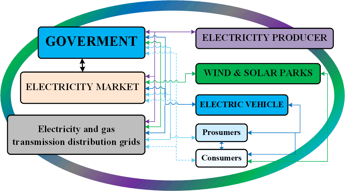
In addition to this structural complexity, system operation involves numerous interacting decision-makers. Decisions are made at different levels (Figure 1) when modeling future energy systems and the operation of their elements, based on a series of forecasts regarding energy production and consumption, climate impact, the use of primary energy resources, and costs. Furthermore, within this process, the best development option is sought.
It should be noted that the illustrations in Figure 1 are simplified and do not account for additional relevant systems, such as neighboring countries’ energy systems, district heating networks, or gas supply infrastructure. In practice, market rules and regulatory frameworks play a central role in shaping actors’ decisions. Each actor must therefore form expectations about the future state of the power system and market conditions, including the anticipated behavior of competitors within these rules. Such expectations are typically represented through a set of scenarios, defined by key parameters reflecting possible future developments. Based on these scenarios, each actor solves an individual planning problem corresponding to the assumed market environment. This representation reflects de-centralized decision-making at the actor level and illustrates how individual planning is guided by scenario-based expectations. The interactions among these actors—and their cumulative effects over time—shape long-term system development in ways that cannot be captured through disaggregated analysis alone. To account for these system-wide dynamics, literature increasingly emphasizes the need for integrated, long-term analytical frameworks. Strategic energy planning has emerged as a key approach in this context, providing tools to assess how different investment pathways, policy choices, and techno-logical developments influence the evolution of the energy system as a whole [16,17,18].
1.3. Objectives and Performance Variables
Strategic energy planning [19] is a comprehensive methodology to guide long-term investments in energy infrastructure. It inherently relies on capacity expansion planning and modelling, which enable the simulation and optimization of future energy system configurations under various policies, technological, and demand scenarios [2,17].
The primary objective of strategic energy planning is to optimize long-term system performance. This objective is not limited to a single metric, but rather reflects a combination of economic, technical, and policy-related criteria. In many modelling approaches [20,21,22,23], it is formulated as the maximization of expected profit or, equivalently, the minimization of total system costs, which provides a tractable representation of system-wide efficiency. More generally, profit can be interpreted as a composite performance measure that aggregates multiple economic and system-level components, including revenues, operational costs, investment expenditures, and, where relevant, reliability indicators and policy-related incentives or penalties. At the same time, it is acknowledged that strategic energy planning is inherently multi-objective, and alternative formulations may explicitly incorporate additional objectives such as environmental sustainability, security of supply, or social welfare.
In this paper, the term profit is adopted as a generalized objective function, with the understanding that alternative optimization objectives could be used in its place. The key requirement is that such objectives can be formally represented within a unified mathematical framework, as expressed in Equation (1). Accordingly, the objective function can be written in profit-maximization form as
where:
- x denotes the vector of decision variables, such as investment and operational decisions, belonging to the feasible set X(S). The vector x may include time-varying variables, for example taxation levels, generation outputs at each time step, or investment decisions such as generation and grid capacities. These variables should be specified at a sufficiently high temporal resolution, for example hourly or finer, over a multi-year planning horizon. The set X(S) denotes the feasible region for x, typically defined by technical, physical, economic, and regulatory constraints. Thus, the constraints of the optimization problem are represented implicitly through the definition of X(S).
- The random input process ξ (e.g., energy demand, weather conditions, market prices) is multidimensional and time-dependent and represents exogenous uncertainty. Such processes can exhibit diverse temporal patterns, including hourly, daily, and seasonal variations, as well as purely stochastic fluctuations, depending on the system under study and the external driving factors.
- s∈S denotes the scenario descriptors, including structural configuration of the system, installed capacities, network topology, and long-term constraints. The feasible set S contains all configurations that satisfy the relevant technical, economic, and regulatory requirements. The configuration may be time-dependent, i.e., s=s(t). Building on this, the feasible set X of operational decisions depends on external scenario-defining parameters. Accordingly, it is written as x(s)∈X(S), where s now denotes the scenario descriptors characterizing external conditions such as demand trajectories, fuel prices, technological costs, or policy settings. These descriptors may be specified exogenously by the decision maker or, in some formulations, treated as additional variables and optimized jointly with x. Set S may be represented either as a finite collection of deterministic scenarios or as a continuous uncertainty set describing the admissible range of uncertain parameters. Typically, these descriptors capture long-term forecast uncertainties, such as the growth of energy consumption and generation or evolutions in energy prices.
- Π(x(s), ξ) is a real-valued measurable function mapping decisions and uncertainty realizations to outcomes (e.g., profit, cost, utility). Hereafter, profit denotes the chosen performance indicator serving as the optimization objective.
- 𝔼[Π(x(s),ξ)] is the risk-neutral objective, representing the expected performance under the probability distribution of ξ.
In practice, the problem under consideration is further complicated by the presence of multiple decision-makers (agents) Figure 2. Each agent formulates an individual optimization problem, through which it defines its specific objectives and performance indicators, including profit, and determines its own set of decision variables.
The planning problem (1) often covers substantial computational and modelling challenges [5]. When the planning task encompasses the coordinated development of the entire power system—generation, transmission, storage, and supporting infrastructure—the resulting optimization problem becomes particularly demanding. Even for relatively small power systems, the dimensionality of the problem can be very high due to the time resolution (e.g., hourly or sub-hourly decisions over a full decade’s long planning period) and the number of decision variables. Moreover, the problem is typically nonlinear, with non-convexities introduced by technical constraints, system dynamics, and the stochastic nature of inputs. As a result, the maximization procedure becomes complex and computationally intensive [6]. Indeed, the general form of expected profit maximization can be expressed as an integral, which highlights the challenge of accounting for all possible realizations of the random inputs: Specifically, the problem can be formulated as:
where:
p(ξ) is its probability density function. Integral (2) is hard to compute when p(ξ) is unknown or intractable; ξ is high-dimensional and Π(x(s),ξ) is nonlinear, which is typical in many practical stochastic optimization problems.
That's why sample-based approximations like Sample Average Approximation (SAA) [24] or ergodic Time-Averaged Approximation (TAA) are broadly used [25]. The SAA is a method for approximating the expected value using a finite number of sampled scenarios. Instead of solving the original problem (1), you solve the SAA problem:
where:
are N independent scenario trajectories (time series realizations); is the sample average approximation of the expected profit; N is the sample size.
While SAA offers a useful way to approximate the expected profit, its effectiveness hinges critically on the number of scenarios N used [19]. To alleviate the computational challenges, an alternative approach is to exploit the temporal structure of the problem by using time averaging approximation. Instead of sampling many independent scenarios across the full uncertainty space, time averaging approximation make use of long historical time series – such as hourly data over one or multiple years – to represent the variability of inputs like demand, weather, or prices. If the underlying stochastic process ξt is ergodic and the time horizon T is sufficiently long, the time average converges to the ensemble (statistical) expectation [25].
In this case, the expectation of profit over the random input process ξ is approximated by a time average:
While the TAA eliminates the need for repeated sampling of exogenous stochastic factors, the resulting strategic planning problem remains computationally demanding. This challenge is compounded in practical applications, where the problem is often naturally formulated as a non-cooperative multi-agent decision problem in which each agent seeks to maximize its own expected profit [26].
Formally, let each decision maker i∈I choose a decision vector xi from a feasible set Xi, while the resulting profit depends not only on its own decisions but also on the decisions of competitors x−i. The profit function of the agent i can therefore be written as
where x-i denotes the vector of decisions of all other agents. Since competitor decisions are generally unknown at the planning stage, each agent must evaluate its strategy under multiple possible realizations of x-i. These alternative realizations represent different assumptions regarding competitor behavior and, when combined with stochastic inputs ξ, naturally define a set of scenarios that must be analyzed to assess the expected profitability of a candidate strategy.
From the perspective of agent i, both the competitor decisions x−i and the stochastic inputs ξ represent uncertain external influences. In the context of time-averaged evaluation, these influences can be naturally represented as time series and treated jointly as scenario realizations.
A single scenario can be defined as
where:
x−i represents a specific realization of competitors’ decisions, and ξ denotes a realization (i.e., a sample path) of the underlying stochastic processes over the planning horizon.
These two sources of uncertainty—strategic interactions and exogenous stochastic variability—are treated jointly and represented in a unified manner through the scenario definition. The set S therefore denotes the scenario space, i.e., the collection of all considered realizations of uncertain external influences. In practice, S is constructed by the decision maker to reflect relevant assumptions regarding competitor behavior and stochastic system conditions.
Within this framework, the strategic planning problem can be interpreted as the search for decisions that are robust or optimal with respect to a set of possible competitor actions and stochastic outcomes. Each realization s∈S defines a distinct strategic environment characterized by the joint occurrence of competitor decisions and exogenous uncertainty.
Consequently, profitability must be evaluated for each agent across all feasible combinations of scenario descriptors and stochastic realizations. In other words, for every candidate decision xi of agent i, the corresponding profit must be assessed over the entire scenario set s = {x−i,ξ}. Since the number of possible combinations of scenario descriptors can be exceedingly large, the scenario space rapidly becomes intractable, resulting in a prohibitive computational burden that severely limits both performance evaluation and strategic decision making.
The aforementioned challenges have prompted the development of a range of platforms, frameworks, and tools designed to support the simulation of energy systems and the assessment of their profitability.
1.4. Profit and Cost Estimation in Practice
Energy system simulations, particularly those focused on long-term planning, have been extensively studied in the literature [13,14,15,17,18,30]. Among the many specialized tools developed for these purposes are, for example, MESSAGE, MARKAL, PLEXOS, TIMES, GENeSYS-MOD, and LUT Energy System Transition Model [19], support detailed large-scale system representation and welfare-optimizing planning. In this context, social welfare represents the net economic benefit generated by the power system and is typically defined as the sum of consumer and producer surplus. Consumer surplus reflects the difference between consumers’ willingness to pay and the market price, while producer surplus corresponds to the difference between market revenues and production costs (i.e., the margin between price and marginal cost over the dispatched output). The use of social welfare as the objective function enables the formulation of the planning problem as a single-objective optimization task. Accordingly, these models maximize total social welfare over a given time horizon, subject to system and operational constraints.
Formally, the planning problem is formulated as the maximization of expected social welfare over the scenario set S [33,34]:
where the social welfare function is defined as:
Here, CSi,t and PSj,t denote the consumer and producer surplus associated with consumer i and producer j at time step t, respectively, while I and J represent the total number of consumers and producers. The scenario descriptor s∈S s is defined as:
where ξ captures exogenous (physical) uncertainty, such as demand, renewable generation, and fuel prices, while xb denotes the bids submitted by market participants [35]. These bids characterize the strategic offers submitted to the day-ahead market and reflect participants’ expectations regarding market conditions, anticipated outcomes, and revenue-maximizing behavior. From the perspective of an individual planner, both components are treated as uncertain inputs to the market-clearing process.
The decision variables are scenario-dependent, x=x(s), and must satisfy:
where X(s) denotes the feasible set determined by system and operational constraints, and Xb restricts decisions to admissible market bids.
The constraint x(s)∈Xb introduced in (8) restricts decision variables to feasible market actions derived from bids submitted to the day-ahead electricity market. This formulation reflects actual market practice, in which bidding and market-clearing procedures are executed on a daily basis. The set Xb represents all admissible combinations of bids from market participants, including generators, consumers, and prosumers. Each bid specifies a quantity of electricity to be supplied or consumed, together with an associated price, typically defined on an hourly or sub-hourly basis.
As illustrated in Figure 3, forecasting and scenario generation provide inputs to system simulations, which enable the evaluation of system performance, objectives, optimal configurations, and decision variables under given assumptions. This framework is referred to as the conventional approach. According to Figure 3, the optimization problem is solved conditional on a scenarios and forecasts of stochastic inputs ξi specified by each decision-maker (DMi). In a multi-agent setting, scenarios and input assumptions are defined individually, reflecting heterogeneous expectations and strategic perspectives. Consequently, each DMi faces a distinct realization of exogenous conditions ξi and competitor decisions x−i, resulting in an individualized optimal decision vector .
As illustrated in Figure 3, forecasting and scenario generation provide inputs to system simulations, forming the basis of the conventional optimization framework. This formulation reflects actual market practice, where bidding and market-clearing procedures are performed on a daily basis. However, substantial difficulties arise when the framework is extended to long-term planning problems involving multiple decision-makers.
In a multi-agent setting, the optimization problem is solved conditional on a scenarios and forecasts of stochastic inputs ξi, which are specified independently by each decision-maker. Consequently, the challenge becomes not only conceptual but also computational. Although the feasible set Xb is shared among all agents, each decision-maker constructs their own scenarios and input assumptions, reflecting heterogeneous expectations, forecasting methods, and strategic perspectives. As a result, agents solve distinct optimization problems conditioned on their individual realizations of exogenous inputs ξi and anticipated competitor decisions x−i, leading to different optimal decision vectors .
The complexity further increases in long-term settings, where uncertainty accumulates over time and the dimensionality of the scenario space grows rapidly. When combined with strategic interactions among multiple agents, this results in a substantial increase in computational burden, making direct solution approaches increasingly difficult to apply in practice.
From a practical standpoint, this heterogeneity substantially increases the number of scenarios that must be evaluated to assess profitability. Each DM must repeatedly solve the optimization problem across multiple scenarios to capture uncertainty and strategic interactions. Consequently, the main difficulty is not only the decentralized and belief-dependent nature of the problem, but also the high computational cost associated with large-scale scenario analysis.
This motivates the need for approaches that reduce the computational burden of scenario-based profitability assessment for individual agents, for example by limiting the number of required simulations, simplifying scenario representations, or improving the efficiency of the optimization procedure, while still preserving sufficient accuracy in the evaluation of outcomes.
1.5. Computational Complexity and the Need for Efficient Methods
The computational burden associated with long-term power system planning becomes substantial when profitability must be evaluated across numerous scenarios and interacting decision-makers. Since each stakeholder may employ different assumptions regarding future system evolution, repeated simulation-based evaluations become computationally expensive.
To address this challenge, an artificial neural network (ANN)-based surrogate model is introduced to approximate the profitability function Π(x, ξ). Surrogate enables scalable evaluation across large scenario spaces while significantly reducing computational effort.
Figure 4 illustrates the proposed multistage planning framework. The Framework Creator (FC) defines the long-term vision of the future power system and specifies the range of possible future developments rather than a single deterministic forecast. In this way, the FC establishes the scenario space by identifying plausible boundaries for demand growth, generation expansion, fuel and electricity prices, interconnection capacities, and other uncertain parameters. FM and SG provide inputs to the power system market model, whose outputs are collected into a dataset used to train the ANN surrogate. Once trained, the ANN provides fast approximations of scenario-dependent performance indicators, supporting decision-making related to objectives, structures, and parameters. Unlike the conventional framework shown in Figure 4, where decision-making relies on repeated direct simulations, the proposed approach replaces computationally intensive evaluations with surrogate-based approximations.
Although the computational challenges of long-term planning are widely recognized, relatively few studies have addressed them using dedicated surrogate models. Data-driven surrogate models learn the behavior of detailed simulation models from generated datasets and can efficiently approximate system responses under alternative scenarios [19,20,21,22,23,24,25]. This capability enables extensive simulation and optimization studies that would otherwise be computationally prohibitive.
In the present study, ANN-based surrogate models are developed to represent long-term planning interests while accounting for heterogeneous stakeholder expectations regarding future power system evolution. The surrogate approximation is formulated as
where FANN denotes the neural-network approximation mapping decision variables x and scenario descriptors s(ξ,xb)) to the corresponding performance indicators i (x, ξ). By replacing repeated high-fidelity simulations with ANN approximations, the proposed framework enables efficient analysis of large-scale planning problems while preserving the representation of diverse stakeholder perspectives.
The following section introduces the methodological framework proposed in this work and describes the ANN-based surrogate modeling approach in detail.
1.6. Contribution and Structure
The main contributions of this paper are as follows:
- A novel surrogate-assisted framework for multi-agent strategic energy planning that explicitly represents heterogeneous market participants and their boundedly rational decision behavior. The framework evaluates market outcomes through performance indicators defined as annual expectations estimated using a time-averaging approach, enabling consistent comparison across planning scenarios.
- A methodology for constructing artificial neural network-based surrogate models that integrate multiple planning perspectives and agents’ objectives, while accurately approximating market-driven performance indicators. These indicators represent expected annual outcomes derived from time-averaged market simulations, capturing the long-term economic effects of strategic decisions across different market participants.
- A computationally efficient approach for evaluating strategic performance indicators, which substantially reduces the computational cost of profit estimation while preserving high accuracy. By approximating annual performance metrics, the approach enables tractable analysis of large scenario sets and supports flexible strategic decision-making. Furthermore, it accommodates decisions made by multiple decision-makers, each of whom can define their own objectives and apply domain-specific knowledge to guide the evaluation process.
The article is organized as follows: Section II presents the proposed methodology, detailing the main components of the algorithms and providing the necessary theoretical background for the methods incorporated into the modelling framework. Section III summarizes the case study, while Section IV discusses the results and provides suggestions for future work.
2. Materials and Methods
2.1. Methodological Framework
This chapter presents a computational framework for multi-agent energy planning under stochastic uncertainty and heterogeneous stakeholder expectations. Building upon the ANN-based surrogate modeling approach introduced in the previous section, the framework is designed to support efficient evaluation of strategic decision-making in large-scale long-term planning problems. The proposed methodology consists of three main components.
First, a detailed multi-agent model of the electric power system and electricity market (PSMM) is employed to capture temporal dynamics and strategic interactions among multiple decision-makers operating within a shared market environment. Each agent—representing an existing or prospective asset owner—is associated with a specific portfolio of system elements (e.g., generation, storage, transmission and consumption units) and is characterized by its own state variables, decision variables, and resulting profitability indicators. State variables represent exogenous factors beyond the agent’s control, such as market conditions, system states, competitor behavior, and stochastic drivers (e.g., demand, fuel prices, and renewable generation). Decision variables are endogenously determined within feasible ranges defined by technological and economic constraints.
The model produces both system-level and stakeholder-specific outputs. At the system level, it maximizes social welfare (see (8)) by determining market-clearing prices, dispatch schedules, power flows, and total system costs. The resulting market outcomes define the quantities of energy produced or consumed and the corresponding market prices for each time period. Based on these outputs, revenues and operational costs can be evaluated over individual hours or aggregated across longer planning horizons to construct profitability indicators Π for the considered agents (stakeholders). This agent-based model is used to generate a dataset for surrogate modeling. Although the formulation in (8) resembles a conventional optimization problem, it is not solved to optimality. Instead, it is employed as a conditional performance evaluation operator, whereby state and decision variables are sampled within their feasible domains and each configuration is evaluated via simulation. The resulting input–output pairs establish a functional relationship between decision variables, system states, and performance measures Π, forming the dataset used to train the surrogate model. Simulation outputs are aggregated into representative performance indicators to reduce dimensionality. The dataset thus consists of scenario-dependent profitability measures derived from simulated market outcomes.
The long-term system performance is assessed by simulating the market-clearing procedure on an hourly basis over the multi-year planning horizon. The underlying market mechanism is a centralized day-ahead clearing process based on social welfare maximization, in which supply and demand bids are matched under a uniform pricing scheme. Market participants form price expectations and submit bids subject to operational and market constraints, while the market operator performs the welfare-maximizing clearing, determining both market prices and dispatch decisions. As such mechanisms are standard in the literature and widely implemented in markets such as Nord Pool [36], further details are omitted.
Second, to reduce the computational burden associated with detailed large-scale power system simulations and extensive scenario evaluation, a data-driven surrogate modeling approach is anticipated. Specifically, the surrogate model approximates the mapping between agents’ decision variables, system conditions (state variables), and the resulting performance indicators obtained from detailed power system and market simulations.
Importantly, the performance indicators Π(x,ξ,xb) are scenario-dependent, i.e., they are evaluated for specific realizations of uncertain parameters ξ. As a result, they represent the profitability of each individual agent under a given scenario, rather than aggregated system-level outcomes.
To this end, a dataset D is generated by evaluating the original model across multiple combinations of decision variables and scenario realizations. The scenarios are sampled from a scenario space S, which is designed to cover all stages of the planning horizon and span feasible combinations of uncertain parameters, ensuring that the training data adequately represents the underlying uncertainty. This enables the surrogate model to learn the conditional relationships between decisions, uncertainties, and system performance.
The evaluation of Π(x,ξ,xb) and the generation of dataset D can rely on a wide range of available computational tools and simulation models for power system and market analysis. The accuracy of the surrogate model depends on the quality, diversity, and coverage of dataset D, which must sufficiently represent both the uncertainty space and the decision space.
The resulting trained artificial neural network can then be used to rapidly estimate Π(x,ξ,xb) for a large number of new decision–scenario pairs, thereby enabling efficient solution of large-scale planning problems under uncertainty.
Third, a decision-maker-oriented platform is envisioned, designed to be explicitly constructed and parameterized by decision makers based on their individual knowledge, preferences, and expectations. Within this framework, agents define their own objectives and formulate corresponding optimization problems in accordance with their subjective perspectives. This structure enables decision makers to evaluate alternative strategies and identify preferred solutions using self-selected performance criteria. Each agent assesses the profitability of its decisions based on its expectations regarding the future state of the power system, as well as its specific problem formulation. The detailed formulation of this component is omitted, as it follows established approaches. The emphasis here is on enabling fast and computationally inexpensive evaluation of the objective function, which significantly broadens the range of tractable optimization tasks.
2.2. Performance Indicators and Variables
The described components are implemented through a sequence of operational modules, which together define the structure of the framework. In total, the framework is organized into eight functional blocks (see Figure 5), each representing a distinct stage of the overall modeling process.
The effective application of the framework presented in Figure 5 begins with outlining FB, SG, PSMM blocks defined by the system structure, core performance indicators, and modeling variables, including the selection and representation of key components such as generators, consumers, and the network. In long-term planning applications, this step also includes the identification and selection of relevant technologies and development options for the main system components over multi-decade planning horizons. At this stage, the main influencing factors, system processes, and interactions are identified together with the corresponding forecasting requirements necessary to represent their future evolution and associated uncertainties. The modeling process must be tailored to the specific characteristics of the power system under consideration; an illustrative example is provided in the case study.
The overall structure of the proposed methodology and the main computational blocks of the algorithm are described in the following sections.
2.3. Model Formulation: The Main Stages
2.3.1. Forecasting Framework and Scenario Descriptor Representation
Forecasting Block (FB) and Scenario Generator (SG). The proposed methodology begins with a forecasting module, hereafter referred to as the Forecasting Block. We assume that the long-term evolution of the power system over the planning horizon can be represented through time-dependent variables, as introduced in (6). These variables capture exogenous drivers of system evolution, including market conditions and the behavior of competing market participants. Their projection relies on well-established forecasting methods commonly used in power system analysis, such as load, price, and renewable generation forecasting [37,38,39,40,41]. Historical records of these processes, represented as time series , are assumed to be available or collectible and serve as the basis for model parameter estimation and scenario generation.
To enable the application of the time-averaging approach, the decision variables x and scenario descriptors s are decomposed along the temporal dimension, with the overall planning horizon partitioned into consecutive one-year intervals. The inherently nonstationary stochastic process is thereby approximated as locally stationary over finite time windows. Within each window, stationary and ergodic estimators are applied to approximate the expected profit . Furthermore, to alleviate the computational burden associated with repeated full-scale simulations, the performance indicators are not evaluated directly. Instead, they are approximated through the conditional expectation of profit-related indicators given the relevant decision and scenario variables, i.e. . This substitution preserves the economic interpretability of the indicators while significantly improving computational tractability in scenario-based analyses. It should be noted that the estimation of the conditional expectation E[Π(x∣s,ξ)] can be performed using sample-based Time Average Approximation (see equation (4)) methods, which do not require explicit specification of the underlying probability distributions. To enable this estimation procedure, appropriate variable preprocessing and representation techniques must be introduced.
To operationalize this framework, all model variables—comprising both decision variables x and scenario descriptors s—are classified into two groups (see Figure 6): quasi-fixed variables and time-varying variables.
Under this decomposition, each variable is represented as
where denotes the empirical annual mean and is treated as a quasi-fixed variable, remaining constant within a given year. The scaling factor σ, which controls the magnitude of variability, is also considered a quasi-fixed variable. In contrast, represents the centered time-varying deviation at hourly resolution. This component captures short-term operational variability and is assumed to preserve the same temporal structure throughout the considered planning interval.
This classification separates long-term strategic characteristics from short-term operational dynamics and establishes the conditions necessary for applying the Time-Average Approximation (see equation (4)).
Quasi-fixed variables, denoted as xqf and sqf, are assumed to remain constant within each one-year planning interval but may vary between intervals. These variables represent long-term strategic decisions and slowly evolving scenario descriptors, including installed generation and storage capacities, infrastructure configurations, and other structural characteristics of the system. They are modeled as uncertain parameters defined over feasibility intervals that must be estimated or forecasted by the planner, reflecting limited knowledge about future system development while preserving bounded rational expectations regarding plausible system configurations. This formulation ensures that structural changes occur only between planning intervals, thereby allowing system processes within each interval to be approximated as stationary.
Figure 7.
Variable Classification Diagram.
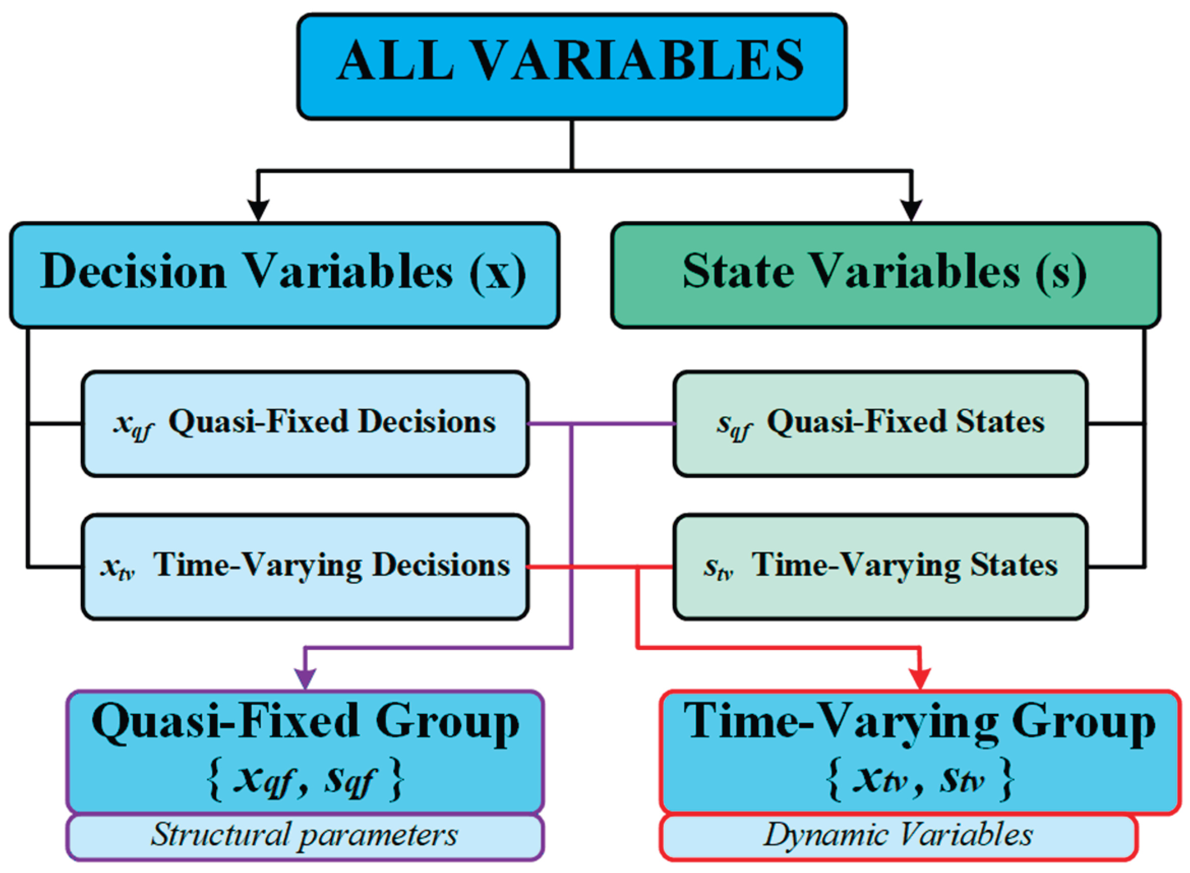
Time-varying variables, denoted as xtv and stv, are defined at a fine temporal resolution (hourly in this study). They represent operational decisions, such as dispatch levels, as well as short-term scenario descriptors, including prices, demand, weather conditions, and resource availability.
Within each one-year planning interval, these variables are modeled using historical recorded processes after centering and normalization. The centered component stv is treated as a stationary stochastic process with zero mean and is modeled using a persistence-based [42] representation derived from centered historical time series. For computational purposes, the resulting processes are represented deterministically as long time series. The original scale and long-term trend of the variables are subsequently reconstructed by combining the centered time-varying component with the quasi-fixed mean values and applying the corresponding scaling factors defined within the feasible space of the quasi-fixed variables. Uncertainty in quasi-fixed (QF) variables is represented through feasibility intervals that define the admissible range of values at each planning stage. It is assumed that the lower and upper bounds of these variables are forecasted in the first planning stage. Let
denote the vector of uncertain variables quasi fixed at stage t, including both exogenous uncertainties and strategic decisions of market participants. The set of all feasible multi-stage realizations is then given by
Thus, S0 defines the feasible uncertainty space over the entire planning horizon. Scenarios are constructed by sampling realizations from this space, such that each scenario corresponds to a point in S0.
Based on this representation, a scenario generator (see Figure 5, block SG) produces a set of scenarios describing possible future states of the power system by means of Monte Carlo sampling, assuming uniform distributions over the feasibility intervals. Each sampled realization s(t)∈S0 consists of simultaneous time series for all components (t).
For each realization s(t), the corresponding multivariate trajectory is provided as input to the Power System and Market Module (block PSMM), which solves the associated operational and market-clearing optimization problem to determine the decision variables x(t). The dataset is constructed by generating a sufficiently large number of scenario descriptors within the admissible space S0. This sampling procedure ensures systematic coverage of the scenario domain and provides representative input data for surrogate model development.
It is important to note that, at this stage, knowledge of the true probability distributions of the scenario parameters is not required. The primary objective is not stochastic optimization itself, but the construction of a surrogate model capable of approximating the relationship between decision variables, scenario descriptors, and performance indicators across the feasible region.
2.3.2. Power System and Market Module
The PSMM constitutes the computational backbone of the strategic planning problem by enabling the consistent integration of power system operation, market mechanisms, and expansion decisions within a unified modeling framework. Owing to the significance and complexity of power system and electricity market planning, problems of this type have been extensively studied in the literature [27,28,29,43]. As a result, a wide range of academic and commercial tools have been developed to support their implementation and analysis, thereby providing flexibility in selecting a modeling platform that is most suitable for the objectives and requirements of a particular study.
In the proposed approach, the PSMM block is not tied to a specific modeling platform; rather, any tool or framework may be employed, provided that if it satisfies a set of essential functional and modeling requirements. Accordingly, the PSMM block must fulfill the following requirements:
- Market-consistent operation: The PSMM shall implement the fundamental electricity market principle by determining operational decisions that maximize social welfare or minimize total system energy supply costs for each given ahead-of-time system state, subject to market rules and technical constraints.
- Comprehensive system representation: The model shall provide an integrated representation of the power system structure, including generation units, storage facilities, and network elements, while accounting for system expansion decisions determined within the planning problem.
- Detailed component modeling: Individual system components and network elements shall be represented with sufficient technical detail to capture their operational characteristics and constraints.
- Explicit market design modeling: Electricity market operation rules (e.g., market clearing mechanisms, pricing schemes, bidding structures) shall be explicitly specified and consistently implemented.
- Constraint verification: All relevant technical, operational, and environmental constraints must be enforced within the optimization framework.
- Performance assessment: The PSMM shall estimate market participants’ performance indicators under specified state-variable conditions using the time-averaging approach defined in Equation (4).
The selected power system structure determines the set of variables that must either be forecasted or treated as state and decision variables within the planning framework. In particular, the system configuration and market design define the relevant state variables (e.g., demand levels, fuel prices, generation profiles, and policy parameters) as well as the decision variables (e.g., investment capacities, generation and consumption dispatch levels, and control policy parameters). Moreover, the selection of performance indicators is jointly determined by the strategic objectives of the decision-makers and the envisioned system structure, reflecting assumptions about the future evolution of the power system, which together define the formulation of the objective function.
2.3.3. Data Repository and Artificial Neural Network [44,45]
The samples generated by the Scenario Generator and the Power System and Market Module (PSMM) are stored and processed in a centralized Dataset Repository DR (see Figure 5). For each generated scenario, the repository records hourly energy volumes for all generators and consumers, together with the common market price per unit of energy. Based on these samples, various performance indicators (∏) can be constructed. In this study, primary attention is given to approximating the expected values of () using the Time-Average Approximation approach presented in (4). By applying the Time-Average Approximation, the dataset collected by the Dataset Repository from the Power System and Market Module is preprocessed before surrogate model construction. In particular, the portion of the dataset used to train the surrogate model is compressed by replacing year-long time series with aggregated performance indicator values, thereby significantly reducing data dimensionality and improving its suitability for artificial neural network training. Specifically, year-long time series are replaced by aggregated performance indicator (Π) values, thereby improving the suitability of the dataset for training ANNs. This reduction significantly decreases the dimensionality of the problem while preserving the information required for accurate surrogate model construction. The training dataset is defined as:
where K denotes the number of simulated scenario samples generated by the Power System and Market Module, and I denotes the number of performance indicators representing the interests of different market participants. The sample size K is selected empirically to balance model accuracy and computational cost; this trade-off is examined in detail in the Case Study chapter. The resulting formulation supports the generation of a large number of scenarios, each corresponding to a specific realization of (xqf,sqf). Collectively, these scenarios constitute the dataset used for ANN training [40,41,46,47]. For each performance indicator, a separate ANN is trained to approximate the conditional mapping defined in (11). During ANN training, the inputs are restricted to the scenario descriptors S0 (see (13) and (14)). Importantly, S0 must be chosen to encompass all plausible visions of different decision makers, ensuring that the surrogate model is robust across diverse planning perspectives. As a result, the trained ANNs approximate the mapping implemented by the PSMM and enable efficient estimation of conditional performance indicators for a wide range of additional user-defined configurations reflecting the individual preferences and strategic objectives of decision-makers, without repeatedly solving the full long-term planning and market simulation problem.
The ANN architectures are selected to provide adequate predictive accuracy; however, the optimization of network structure is beyond the scope of this study. The purpose of the case study is solely to demonstrate that one of the widely used ANN training algorithms yields satisfactory results for the considered application. Owing to the extensive literature on ANN design and training, the reader is referred to [41,46,47,48] for comprehensive reviews. Implementation details and the selected ANN configuration are presented in the case study.
2.3.4. User Scenario Descriptor (USD)
The trained ANN enables rapid evaluation of performance indicators () for agent-defined scenarios, eliminating the need for repeated execution of the detailed Power System and Market Module.
The User Scenario Descriptor module serves as an interface through which agents define scenarios by combining structural decision variables with admissible state descriptors. This formulation enables agents to incorporate heterogeneous information, expectations, and preferences, thereby reflecting both feasible system configurations and individualized strategic perspectives. Consequently, different agents may construct distinct scenario sets even within the same underlying system representation.
The USD module also supports systematic exploration of the admissible solution space, facilitating the identification of preferred configurations according to agent-specific objectives. For each candidate scenario, the corresponding performance indicators are efficiently estimated using the trained ANN surrogate model.
2.3.5. Decision and Optimization Module (DOM)
The Decision Optimization Module constitutes the final layer of the platform, where performance indicators are utilized to formulate and solve a range of optimization problems. Depending on the application, selected performance indicators may be aggregated or transformed into objective functions representing economic, technical, environmental, or risk-related criteria.
Within the DOM, agents can exploit their knowledge of the statistical properties of the underlying variables—such as distributions, correlations, and scenario-dependent variability—to construct customized objective functions. Owing to the computational efficiency of the trained surrogate model, optimization procedures that require a large number of objective function evaluations can be performed efficiently. Furthermore, agents are free to select appropriate optimization algorithms based on the problem structure, computational requirements, and decision-making preferences.
The module supports both single- and multi-objective optimization. In multi-objective settings, customized objective functions may represent a scalarization scheme, weighting rule, or decision criterion applied to the vector of performance indicators. When these indicators reflect the interests of multiple agents, game-theoretic solution concepts—such as the Nash equilibrium or cooperative allocation mechanisms like the Shapley value—can be incorporated to ensure stable and economically consistent outcomes [49].
The Decision and Optimization Module can be viewed as interacting with the User Scenario Descriptor to support the exploration of the decision space. Based on the evaluation of candidate solutions, it may guide the adjustment of decision variables and the generation of new scenarios through the USD, forming a conceptual feedback process that facilitates the identification of agent-specific preferred or near-optimal solutions.
As a result, the DOM module facilitates the application of computationally intensive optimization methods, including search-based algorithms [50] that rely on repeated objective function evaluations. The specific selection, aggregation, and interpretation of performance indicators remain application-dependent and are therefore addressed in the case study.
3. Case Study and Results
3.1. Description of the Considered Power System
The Baltic power system (BPS) has been chosen as the case study to demonstrate the proposed approach. The BPS encompasses the union of the Estonian, Latvian and Lithuanian power systems, with a peak load of approximately 4700 MW [51].
Looking ahead to 2050, a major transformation of the BPS is not only planned but already well underway [52,53]. High-capacity solar and wind power plants will be developed, while facilities that produce significant carbon emissions will be phased out. The structure of the model used in this study is shown in Figure 8.
Depicted structure includes: hydropower plants (HP), pumped storage hydropower plants (PSHP), solar power plants (SPP), wind power plants (WPP), reserve power plants for maintaining energy balance (Reserve), combined heat and power plants (CHPP), and DC and AC interconnections, It incorporates key changes outlined in the National Climate and Energy plans and long-term energy system development strategies [54].
Let us assume that the list of possible changes can be represented by a number of scenarios. These scenarios involve a significant increase in power demand and the capacity of generators. We aim to demonstrate the effectiveness of the proposed approach.
3.2. Operationalization of the Planning Strategy
At the outset of this study, we establish a conceptual vision of the power system under development and define its structural configuration (see Figure 8). This is followed by the selection of performance indicators (Π), such as the average annual zonal electricity price, as well as the quantities and associated costs of energy generated, consumed, and transmitted by individual market participants or groups of participants. We also define the decision-makers, decision variables x, and the forecasting and scenario development framework.
We then construct a long-term, time-varying stochastic input process, ξ, and define the corresponding scenario bounds, S0 (see Table 1). The process ξ is derived from high-resolution (hourly) historical time-series data and extrapolated through 2050. It incorporates projections of electricity demand, river inflows for hydropower generation, solar electricity generation, wind power generation, and electricity prices in interconnected neighboring power systems. A significant increase in energy consumption is projected, along with the planned expansion of solar and wind farms and the construction of a nuclear power plant.
Examples of the resulting stochastic processes [55] are presented in Figure 9 and Figure 10, details are accessible in [56,57,58]. Future trends are estimated using appropriate forecasting methods (see [54,59,60] for methodological details), and the resulting components are structured in accordance with (11). All variables are classified into time-varying and quasi-fixed categories. Each variable is defined within a specified existence interval, restricted by its minimum Smin and maximum Smax values (presented in Table I The parameter ranges are defined subjectively and intentionally chosen to be sufficiently wide to ensure adequate representation of uncertainty. These intervals are subsequently utilized within a Monte Carlo sampling framework to generate realizations of S across the prescribed uncertainty space. A more refined specification of these intervals could be achieved through the application of surrogate modeling techniques.
Assuming that all scenario descriptors are uniformly and independently distributed within known limits, samples of their vector components are generated in a multidimensional space. In this study, the most influential descriptor ranges are summarized in Table I.
The Power System and Market Model is executed sequentially on a daily basis over the entire planning horizon, enabling the representation of cumulative and dynamic effects arising from operational decisions and system constraints. Based on the resulting market outcomes, a set of performance indicators, ∏(S), is computed, including consumer expenditures, installed and utilized generation capacities, investment volumes, and individual generation unit revenues. Such models are well-established in the literature [66,67,68,69]. In this paper, we use the tool described in our previous articles [68,70], However, the proposed methodology is not tool-specific and can be implemented using any approach capable of simulating generation scheduling in power systems with heterogeneous generation and storage technologies over long-term horizons. Market outcomes are determined through a linear programming formulation that captures bidding behavior, generation dispatch, and the market-clearing process. The model emulates the actions of a market operator by selecting the least-cost generation portfolio subject to system balance and network constraints. Electricity market bids are generated on an hourly basis using forecasted time series and scenarios throughout the simulation period. Prices in neighboring market areas (Poland, Finland, Sweden) are assumed to be forecasted with hourly resolution, and reserve power plants are activated only when required to maintain system balance. Renewable generators are modeled as price-takers with near-zero marginal production costs. Consequently, they adopt a bidding strategy aimed at ensuring dispatch rather than price-setting. For each market interval (e.g., hourly in the day-ahead market), generators submit bids equal to their forecasted production quantities at prices close to zero. This reflects their economic incentive to maximize acceptance in market clearing while minimizing curtailment risk. Hydropower plants are modeled taking into account water inflows and environmental restrictions [71,72,73,74]. Reserve power plants are activated only when renewable sources and storage cannot fully satisfy demand. The price of reserve energy is treated as a quasi-constant parameter. Nuclear power plants are modeled as inflexible baseload units characterized by high fixed costs and low marginal operating costs. Due to technical and economic constraints (e.g., limited ramping capability and high cycling costs), they operate at near-constant output levels. Accordingly, nuclear generators submit bids corresponding to their available capacity at zero (or near-zero) price to ensure continuous dispatch. This strategy reflects their preference for stable operation and revenue certainty over short-term price optimization.
ANN. In this study, we applied a Feed-Forward Neural Network (FFNN) – a well-established ANN architecture widely used in scientific research [75]. The training process of the ANN is carried out using the Levenberg–Marquardt optimization algorithm, which is known for its efficiency in minimizing the error surface during back-propagation training. The performance of the training is evaluated using the Mean Squared Error metric, which is a standard approach for assessing regression accuracy in ANN-based forecasting models. In the task under consideration, multiple performance indicators Πi may be required, and a separate ANN is constructed for each indicator. This separation is appropriate because each Πi is typically associated with a particular decision maker and reflects that agent’s specific objective function, decision variables, scenario descriptors, and feasibility constraints. Since the planning problem involves multiple decision makers, each with potentially different objectives and constraints, the corresponding performance indicators may exhibit substantially different functional dependencies. Once trained, each ANN enables rapid evaluation of the associated performance indicator, eliminating the need to repeatedly solve the underlying computationally intensive optimization problem.
The selected ANN architecture consists of an input layer, two consecutive hidden layers with 20 neurons each, and a single output layer. This configuration was determined according to our previously developed methodology [41] and was implemented using the Matlab 2024a software package.
3.3. Sample Inputs for Planning Task Scenarios
An example of the resulting samples of scenario descriptors, projected onto a representative three-dimensional subspace of the full input space, are illustrated in Figure 11
Using the obtained values of scenario descriptors and realizations of random processes from dataset D, we generate a set of estimates for the conditional annual averages of profits or expenses Πi (see equations (5), (6)). It is essential to mention that the results depicted in Figure 11 may raise questions or queries, as the samples generated using a large uniform distribution of variables. Some combinations of scenario descriptors may be unlikely in practice. However, these sampled results are used solely for training the ANN.
The accuracy of Πi estimation ultimately depends on the quality of information available to decision makers, as their strategic behavior directly shapes the input data. Accordingly, the predictive accuracy of the ANN can be enhanced by incorporating scenario descriptors provided by well-informed decision makers, who construct their optimization problems based on assumed probability distributions of these descriptors. This integration enables the model to better reflect realistic expectations and uncertainty perceptions, thereby improving its explanatory and predictive capability.
3.4. A Representative Subset of Πi Estimates
To demonstrate the practical value of the surrogate model, a limited subset of performance indicators Πi and a 16-dimensional scenario descriptor space were selected for the case study. A total of 22,000 samples were generated from the descriptor space. This restriction was introduced solely due to the page limitations of the present article and was not motivated by any computational constraints. Our goal is to show that providing market participants with access to a surrogate model enables them to rapidly solve their own planning tasks. Below, we present a focused set of Πi estimates relevant to key stakeholders, including government bodies (e.g., for import/export analysis), transmission system operators, large power producers, and prosumers. Even this compact selection effectively highlights the core challenges associated with a multitude of scenario descriptors in energy system planning.
The Figure 12 illustrates two Πi – annual incomes and expenses from export and import – calculated for ten combinations of SPP and WPP development scenario descriptors (SPP and WPP installed capacities). The remaining descriptors are taken from the ‘base’ scenario column in Table I. It is important to note that this figure does not represent the estimation of Πi for all possible descriptor combinations. However, such estimations can be readily obtained by enumerating the combinations of interest to the user.
We assume that import and export costs are of particular interest to high-level economic decision makers. Figure 13. shows the annual average import expenditure value as a function from SPP and WPP descriptors.
The subsequent diagram illustrates the profit of various types of electricity producers and expected electricity market price (Figure 14).
It is worth noting that similar estimates can, in principle, be obtained using only the detailed model. However, as will be shown below, this approach entails substantially higher computational costs while offering little to no improvement in accuracy. In contrast, the surrogate model produces results of comparable quality at a significantly reduced computational effort. Its advantages become particularly evident—and increasingly pronounced—as the number of scenarios under consideration grows.
3.5. Time and Accuracy of Indicator Estimation
This section presents an analysis of the time requirements and accuracy of estimating profitability indicators using a detailed and surrogate model. The results obtained using computer with parameters as follow: CPU: Intel i7-4770K 3.50GHz (4 cores), RAM: 32 GB DDR3 GPU NVIDIA GeForce GT 630 RAM: 2 GB
The total computation time for preparing dataset D depends on the number of samples. Each sample requires an individual run of the detailed model. One sample calculation time is about 70 seconds. In that way the total procedure for 20 000 samples takes around 1400000 seconds or 16 days.
An important question arises regarding the number of samples required to ensure accurate approximation by the surrogate model. To address this, numerical experiments were conducted in which an artificial neural network was trained using different numbers of samples. The model's accuracy was then evaluated using the Mean Absolute Percentage Error (MAPE) metric [76]. The results are presented in Figure 15 and Figure 16.
Figure 17 indicates that training the surrogate model with 2,000–3,000 samples is sufficient, as the model performance stabilizes and shows no significant improvement with additional data.
3.6. Model Accuracy and Computation Time
The accuracy of the surrogate model was evaluated by comparing its predictions with the outputs of the detailed model using a separate validation dataset that was not employed during the ANN training phase. Figure 16 illustrates the distribution of MAPE values [77] obtained during the final electricity price verification of the surrogate model against the detailed model. In 73% of the validation cases, the MAPE lies within the range of 0–1%, while the overall procedure results in an average inaccuracy of 1.27%.
A Feed-Forward Neural Network was used for this purpose, with each network taking approximately 0.005 seconds to train. This one-time computational effort enables fast estimations for new scenarios. The result indicates that the training process requires significantly less time compared to the dataset preparation and has a negligible impact on the overall computational cost.
After training, the surrogate model was used to estimate profitability indicators for new input scenarios. The average time per estimation was less than the second, demonstrating the efficiency of the approach compared to the detailed model, which required approximately 70 seconds per run.
4. Discussion
This study develops a surrogate-modelling framework for strategic power-system planning in which Artificial Neural Networks are trained on datasets generated by detailed power-system and market simulations. The surrogate model is then used to approximate profitability and system performance metrics across a large set of long-term development scenarios, thereby reducing reliance on repeated high-resolution operational simulations.
The results indicate that the trained ANN surrogate model reproduces the outputs of the detailed model with an average approximation error below 1.5%. In computational terms, the evaluation time per scenario decreases from tens of seconds to below one second, which materially expands the feasible scope of scenario enumeration and sensitivity analysis. This acceleration is particularly relevant for planning problems characterized by high-dimensional uncertainty and combinatorial design spaces (e.g., technology portfolios, interconnection capacities, and policy constraints).
In the Baltic power system case study, the surrogate model captures key structural dependencies linking generation expansion, cross-border exchanges, and market price formation. This suggests that the learning procedure preserves the dominant input–output relationships embedded in the underlying operational and market logic, supporting its use in multi-decade transition assessments where numerous candidate configurations must be compared consistently.
Methodologically, the main contribution is the integration of an explicit profit (or cost) estimation layer into long-term planning workflows, designed to reflect the influence of short-term operational behavior on long-term economic outcomes. By combining model decomposition with surrogate modelling, the framework embeds the effect of operational optimization within strategic evaluation without requiring full high-resolution dispatch simulation for each scenario.
A deliberate simplification is the use of aggregated annual indicators rather than full temporal operational trajectories. While this choice reduces the representation of short-term variability and extreme events at the strategic screening stage, it enables scalable analysis and is defensible when the primary objective is comparative evaluation of many structural alternatives. Nevertheless, this modelling choice implies that additional verification with temporally resolved simulations may be required for shortlisted scenarios, especially where adequacy, congestion, or scarcity pricing in rare hours materially affects conclusions.
Although the empirical demonstration focuses on a relatively small power system, the test set includes substantial structural changes and a diverse set of technologies (generation, storage, and cross-border options). This provides initial evidence that the approach is not restricted to incremental modifications. Its modular structure and computational efficiency make it transferable to larger and more complex systems, provided that the training data sufficiently covers the relevant operating regimes and that validation is repeated under expanded conditions.
5. Conclusions
An ANN-based surrogate model can be used as an effective approximation layer for long-term power-system planning when trained on outputs from detailed power-system and market simulations. In the demonstrated application, the surrogate achieves an average approximation error below 1.5% while reducing per-scenario evaluation time from tens of seconds to less than one second, enabling extensive scenario exploration and uncertainty analysis.
The proposed framework enhances strategic planning by accounting for short-term operational behavior in long-term economic assessment without executing high-resolution dispatch for every scenario. The approach is therefore suitable as an optimization-ready screening tool and a decision-support component for planners, regulators, and researchers, with the proviso that temporally resolved verification remains important for final design selection, particularly under conditions of high variability in electricity prices, demand, and renewable generation.
Author Contributions
AS and RP initiated the study; AS, DZ and RP developed the study approach; RP and AS formed the database and executed the simulation and results analysis; AS and DZ drafted the manuscript; GB, KB, EE and RP re-viewed and revised the manuscript.
Funding
This research is funded by the Latvian Council of Science, project No. LZP-2024/1-0568 “Navigating the Baltic Energy System to a Low Carbon Future: A Techno-Economic Exploration of Challenges and Innovative Opportunities (NAVIGATOR)” and project No. LZP – 2023/ 1- 0376 “Innovative emergency control of RES-dominated low-inertia power systems (INNOVA)”. As well, This activity/work has been supported by the EU Recovery and Resilience Facility within the Project No 5.2.1.1.i.0/2/24/I/CFLA/003 “Implementation of consolidation and management changes at Riga Technical University, Liepaja University, Rezekne Academy of Technology, Latvian Maritime Academy and Liepaja Maritime College for the progress towards excellence in higher education, science and innovation” academic career doctoral grant (ID 1013).
Data Availability Statement
The raw data supporting the model used and conclusions of this article will be made available by the authors, without undue reservation, to any qualified researcher.
Conflicts of Interest
The authors declare no conflict of interest.
References
- “Delivering the European Green Deal - European Commission.” Accessed: Jul. 26, 2025. [Online]. Available: https://commission.europa.eu/strategy-and-policy/priorities-2019-2024/european-green-deal/delivering-european-green-deal_en.
- M. Emmanuel, K. Doubleday, B. Cakir, M. Marković, and B.-M. Hodge, “A review of power system planning and operational models for flexibility assessment in high solar energy penetration scenarios,” Solar Energy, vol. 210, pp. 169–180, Nov. 2020. [CrossRef]
- F. Milano, F. Dörfler, G. Hug, D. J. Hill, and G. Verbič, “Foundations and Challenges of Low-Inertia Systems (Invited Paper),” in 2018 Power Systems Computation Conference (PSCC), Dublin, Ireland: IEEE, Jun. 2018, pp. 1–25. [CrossRef]
- A. Sauhats, D. Zalostiba, A. Utans, and R. Petricenko, “Enhancing resilience of low-inertia power systems through a novel load shedding method with synchronous condenser power control,” Environ Syst Decis, vol. 45, no. 3, p. 51, Sep. 2025. [CrossRef]
- L. Kotzur et al., “A modeler’s guide to handle complexity in energy systems optimization,” Advances in Applied Energy, vol. 4, p. 100063, Nov. 2021. [CrossRef]
- J. Priesmann, L. Nolting, and A. Praktiknjo, “Are complex energy system models more accurate? An intra-model comparison of power system optimization models,” Applied Energy, vol. 255, p. 113783, Dec. 2019. [CrossRef]
- H. Majidi et al., “Overview of energy modeling requirements and tools for future smart energy systems,” Renewable and Sustainable Energy Reviews, vol. 212, p. 115367, Apr. 2025. [CrossRef]
- M. Fodstad et al., “Next frontiers in energy system modelling: A review on challenges and the state of the art,” Renewable and Sustainable Energy Reviews, vol. 160, p. 112246, May 2022. [CrossRef]
- M. Chang et al., “Trends in tools and approaches for modelling the energy transition,” Applied Energy, vol. 290, p. 116731, May 2021. [CrossRef]
- S. Mohseni and A. C. Brent, “Long-term planning optimisation of sustainable energy systems: A systematic review and meta-analysis of trends, drivers, barriers, and prospects,” Energy Strategy Reviews, vol. 57, p. 101640, Jan. 2025. [CrossRef]
- G. Aquila, L. B. S. Morais, V. A. D. de Faria, J. W. M. Lima, L. M. M. Lima, and A. R. de Queiroz, “An Overview of Short-Term Load Forecasting for Electricity Systems Operational Planning: Machine Learning Methods and the Brazilian Experience,” Energies, vol. 16, no. 21, p. 7444, Jan. 2023. [CrossRef]
- M. Tostado-Véliz, A. Rezaee Jordehi, S. Amir Mansouri, and F. Jurado, “Day-ahead scheduling of 100% isolated communities under uncertainties through a novel stochastic-robust model,” Applied Energy, vol. 328, p. 120257, Dec. 2022. [CrossRef]
- P. Lopion, P. Markewitz, M. Robinius, and D. Stolten, “A review of current challenges and trends in energy systems modeling,” Renewable and Sustainable Energy Reviews, vol. 96, pp. 156–166, Nov. 2018. [CrossRef]
- T. Horschig and D. Thrän, “Are decisions well supported for the energy transition? A review on modeling approaches for renewable energy policy evaluation,” Energ Sustain Soc, vol. 7, no. 1, p. 5, Feb. 2017. [CrossRef]
- G. Savvidis et al., “The gap between energy policy challenges and model capabilities,” Energy Policy, vol. 125, pp. 503–520, Feb. 2019. [CrossRef]
- M. Howells et al., “OSeMOSYS: The Open Source Energy Modeling System: An introduction to its ethos, structure and development,” Energy Policy, vol. 39, no. 10, pp. 5850–5870, Oct. 2011. [CrossRef]
- D. Huppmann et al., “The MESSAGEix Integrated Assessment Model and the ix modeling platform (ixmp): An open framework for integrated and cross-cutting analysis of energy, climate, the environment, and sustainable development,” Environmental Modelling & Software, vol. 112, pp. 143–156, Feb. 2019. [CrossRef]
- A. Fattahi, J. Sijm, and A. Faaij, “A systemic approach to analyze integrated energy system modeling tools: A review of national models,” Renewable and Sustainable Energy Reviews, vol. 133, p. 110195, Nov. 2020. [CrossRef]
- S. Moret, F. Babonneau, M. Bierlaire, and F. Maréchal, “Decision support for strategic energy planning: A robust optimization framework,” European Journal of Operational Research, vol. 280, no. 2, pp. 539–554, Jan. 2020. [CrossRef]
- “Capacity planning of renewable energy systems using stochastic dual dynamic programming,” European Journal of Operational Research, vol. 322, no. 2, pp. 573–588, Apr. 2025. [CrossRef]
- N. S. Goteti, E. Hittinger, and E. Williams, “Stochastic Capacity Expansion Model Accounting for Uncertainties in Fuel Prices, Renewable Generation, and Demand,” Energies, vol. 18, no. 5, p. 1283, Jan. 2025. [CrossRef]
- “Stochastic long-term joint decarbonization planning for power systems and data centers: A case study in PJM,” International Journal of Electrical Power & Energy Systems, vol. 173, p. 111377, Dec. 2025. [CrossRef]
- A. Brenner, R. Khorramfar, D. Mallapragada, and S. Amin, “Learning-assisted Stochastic Capacity Expansion Planning: A Bayesian Optimization Approach,” 2024. [CrossRef]
- B. Verweij, S. Ahmed, A. J. Kleywegt, G. Nemhauser, and A. Shapiro, “The Sample Average Approximation Method Applied to Stochastic Routing Problems: A Computational Study,” Computational Optimization and Applications, vol. 24, no. 2, pp. 289–333, Feb. 2003. [CrossRef]
- M. Boshernitzan, G. Kolesnik, A. Quas, and M. Wierdl, “Ergodic averaging sequences,” J. Anal. Math., vol. 95, no. 1, pp. 63–103, Dec. 2005. [CrossRef]
- C.-S. Karavas, K. Arvanitis, and G. Papadakis, “A Game Theory Approach to Multi-Agent Decentralized Energy Management of Autonomous Polygeneration Microgrids,” Energies, vol. 10, no. 11, p. 1756, Nov. 2017. [CrossRef]
- S. Jebaraj and S. Iniyan, “A review of energy models,” Renewable and Sustainable Energy Reviews, vol. 10, no. 4, pp. 281–311, Aug. 2006. [CrossRef]
- J. DeCarolis et al., “Formalizing best practice for energy system optimization modelling,” Applied Energy, vol. 194, pp. 184–198, May 2017. [CrossRef]
- D. Bogdanov et al., “Low-cost renewable electricity as the key driver of the global energy transition towards sustainability,” Energy, vol. 227, p. 120467, Jul. 2021. [CrossRef]
- J. P. Deane, A. Chiodi, M. Gargiulo, and B. P. Ó Gallachóir, “Soft-linking of a power systems model to an energy systems model,” Energy, vol. 42, no. 1, pp. 303–312, Jun. 2012. [CrossRef]
- F. Paraschiv, D. Erni, and R. Pietsch, “The impact of renewable energies on EEX day-ahead electricity prices,” Energy Policy, vol. 73, pp. 196–210, Oct. 2014. [CrossRef]
- M. Howells et al., “OSeMOSYS: The Open Source Energy Modeling System,” Energy Policy, vol. 39, no. 10, pp. 5850–5870, Oct. 2011. [CrossRef]
- Y. Xi, Q. Zeng, Z. Chen, H. Lund, and A. J. Conejo, “A market equilibrium model for electricity, gas and district heating operations,” Energy, vol. 206, p. 117934, Sep. 2020. [CrossRef]
- I. A. Puiu and R. A. Hauser, “On market clearing of day ahead auctions for European power markets: Consumer payment minimisation versus social welfare maximisation,” Energy Economics, vol. 139, p. 107880, Nov. 2024. [CrossRef]
- P. Xiong, P. Jirutitijaroen, and C. Singh, “A Distributionally Robust Optimization Model for Unit Commitment Considering Uncertain Wind Power Generation,” IEEE Transactions on Power Systems, vol. 32, no. 1, pp. 39–49, Jan. 2017. [CrossRef]
- “See what Nord Pool can offer you.” Accessed: May 05, 2026. [Online]. Available: https://www.nordpoolgroup.com/en/.
- T. Hong and S. Fan, “Probabilistic electric load forecasting: A tutorial review,” International Journal of Forecasting, vol. 32, no. 3, pp. 914–938, Jul. 2016. [CrossRef]
- J. Zhang et al., “A suite of metrics for assessing the performance of solar power forecasting,” Solar Energy, vol. 111, pp. 157–175, Jan. 2015. [CrossRef]
- R. Weron, “Electricity price forecasting: A review of the state-of-the-art with a look into the future,” International Journal of Forecasting, vol. 30, no. 4, pp. 1030–1081, Oct. 2014. [CrossRef]
- R. Petrichenko, D. Sobolevsky, and A. Sauhats, “Short-Term Forecasting of District Heating Demand,” in Proc. - IEEE Int. Conf. Environ. Electr. Eng. IEEE Ind. Commer. Power Syst. Europe, EEEIC/I CPS Europe, Institute of Electrical and Electronics Engineers Inc., 2018. [CrossRef]
- K. Baltputnis, R. Petrichenko, and A. Sauhats, “ANN-based city heat demand forecast,” in 2017 IEEE Manchester PowerTech, Manchester, United Kingdom: IEEE, Jun. 2017, pp. 1–6. [CrossRef]
- A. K. Bansal, “Sizing and forecasting techniques in photovoltaic-wind based hybrid renewable energy system: A review,” Journal of Cleaner Production, vol. 369, p. 133376, Oct. 2022. [CrossRef]
- A. J. Conejo, M. Carrión, and J. M. Morales, Decision Making Under Uncertainty in Electricity Markets, vol. 153. in International Series in Operations Research & Management Science, vol. 153. Boston, MA: Springer US, 2010. [CrossRef]
- A. Mosavi, M. Salimi, S. Faizollahzadeh Ardabili, T. Rabczuk, S. Shamshirband, and A. R. Varkonyi-Koczy, “State of the Art of Machine Learning Models in Energy Systems, a Systematic Review,” Energies, vol. 12, no. 7, p. 1301, Jan. 2019. [CrossRef]
- R. Islam, M. A. H. Rivin, S. Sultana, M. A. B. Asif, M. Mohammad, and M. Rahaman, “Machine learning for power system stability and control,” Results in Engineering, vol. 26, p. 105355, Jun. 2025. [CrossRef]
- “What is a neural network? | Types of neural networks.” Accessed: Sep. 15, 2025. [Online]. Available: https://www.cloudflare.com/learning/ai/what-is-neural-network/.
- J. Ferrero Bermejo, J. F. Gómez Fernández, F. Olivencia Polo, and A. Crespo Márquez, “A Review of the Use of Artificial Neural Network Models for Energy and Reliability Prediction. A Study of the Solar PV, Hydraulic and Wind Energy Sources,” Applied Sciences, vol. 9, no. 9, p. 1844, Jan. 2019. [CrossRef]
- “feedforwardnet - Generate feedforward neural network - MATLAB.” Accessed: Sep. 15, 2025. [Online]. Available: https://se.mathworks.com/help/deeplearning/ref/feedforwardnet.html.
- W. Tushar, T. K. Saha, C. Yuen, D. Smith, and H. V. Poor, “Peer-to-Peer Trading in Electricity Networks: An Overview,” IEEE Transactions on Smart Grid, vol. 11, no. 4, pp. 3185–3200, Jul. 2020. [CrossRef]
- G. Zhang, Y. Ge, Z. Ye, and M. Al-Bahrani, “Multi-objective planning of energy hub on economic aspects and resources with heat and power sources, energizable, electric vehicle and hydrogen storage system due to uncertainties and demand response,” Journal of Energy Storage, vol. 57, p. 106160, Jan. 2023. [CrossRef]
- G. H. Valencia-Rivera et al., “A systematic review of metaheuristic algorithms in electric power systems optimization,” Applied Soft Computing, vol. 150, p. 111047, Jan. 2024. [CrossRef]
- “National Energy and Climate Plan for 2021-2030 | Ekonomikas ministrija.” Accessed: Jul. 25, 2025. [Online]. Available: https://www.em.gov.lv/en/national-energy-and-climate-plan-2021-2030.
- A. Sauhats, Z. Broka, and K. Baltputnis, “Energy Transition of the Baltic States: Problems and Solutions,” LPTS, vol. 58, no. 3, pp. 3–14, Jun. 2021. [CrossRef]
- J. Carvallo, N. Zhang, B. Leibowicz, T. Carr, S. Baik, and P. Larsen, “A Guide for Improved Resource Adequacy Assessments in Evolving Power Systems: Institutional and Technical Dimensions,” None, 1987650, ark:/13030/qt4dq364g2, Jun. 2023. [CrossRef]
- A. Sauhats, R. Petrichenko, and M. Zima-Bockarjova, “A Pragmatic Approach to the Economic Assessment of Green Synthetic Methane Power in the Baltics,” Energies, vol. 16, no. 22, 2023. [CrossRef]
- “ENTSO-E Transparency Platform.” Accessed: Jul. 25, 2025. [Online]. Available: https://transparency.entsoe.eu/dashboard/show.
- L. Petrichenko, R. Petrichenko, A. Sauhats, K. Baltputnis, and Z. Broka, “Modelling the Future of the Baltic Energy Systems: A Green Scenario,” Latvian Journal of Physics and Technical Sciences, vol. 58, no. 3, pp. 47–65, Jun. 2021. [CrossRef]
- R. Petrichenko, L. Petrichenko, A. Sauhats, A. Slivikas, S. Gudzius, and M. Zima-Bockarjova, “Profitability Study of Floating PV and Storage Pumped Hydropower Plant,” in Int. Conf. European Energy Market, EEM, IEEE Computer Society, 2020. [CrossRef]
- R. Petrichenko, J. Kozadajevs, L. Petrichenko, and A. Silis, “Reserve power estimation according to the Baltic power system 2050 development plan,” in ENERGYCON - IEEE Int. Energy Conf., Proc., Institute of Electrical and Electronics Engineers Inc., 2022. [CrossRef]
- European Commission. Directorate General for Mobility and Transport., Ref4e., Mercados., and E bridge., Identification of appropriate generation and system adequacy standards for the internal electricity market: final report. LU: Publications Office, 2014. Accessed: Sep. 10, 2025. [Online]. Available: https://data.europa.eu/doi/10.2832/089498.
- A. Sauhats, R. Varfolomejeva, R. Petrichenko, and J. Kucajevs, “A stochastic approach to hydroelectric power generation planning in an electricity market,” in 2015 IEEE 15th International Conference on Environment and Electrical Engineering (EEEIC), Jun. 2015, pp. 883–888. [CrossRef]
- “Estonia starts planning process for SMR plant,” World Nuclear News. Accessed: Sep. 16, 2025. [Online]. Available: https://world-nuclear-news.org/articles/estonia-starts-planning-process-for-smr-plant.
- F. Media, “Kruonis Pumped Storage Hydroelectric Power Plant (KPSHP) | Ignitis gamyba,” Kruonis Pumped Storage Hydroelectric Power Plant (KPSHP) | Ignitis gamyba. Accessed: Apr. 17, 2026. [Online]. Available: https://ignitisgamyba.lt/en/our-activities/electricity-generation/kruonis-pumped-storage-hydroelectric-power-plant-kpshp/4188.
- “Nord Pool Electricity Prices - Energy Market Data.” Accessed: May 13, 2026. [Online]. Available: https://nordpool.lv/.
- “BTD.” Accessed: May 13, 2026. [Online]. Available: https://baltic.transparency-dashboard.eu/.
- “GridView | Hitachi Energy.” Accessed: Mar. 01, 2026. [Online]. Available: https://www.hitachienergy.cn/cn/zh/products-and-solutions/energy-portfolio-management/enterprise/gridview?utm_source=chatgpt.com.
- “Aurora Energy Forecasting and Analysis Software | Energy Exemplar.” Accessed: Mar. 01, 2026. [Online]. Available: https://www.energyexemplar.com/aurora.
- T. Hong, P. Pinson, Y. Wang, R. Weron, D. Yang, and H. Zareipour, “Energy Forecasting: A Review and Outlook,” IEEE Open J. Power Energy, vol. 7, pp. 376–388, 2020. [CrossRef]
- T. Ahmad, H. Zhang, and B. Yan, “A review on renewable energy and electricity requirement forecasting models for smart grid and buildings,” Sustainable Cities and Society, vol. 55, p. 102052, Apr. 2020. [CrossRef]
- M. Papadimitrakis, N. Giamarelos, M. Stogiannos, E. N. Zois, N. a.-I. Livanos, and A. Alexandridis, “Metaheuristic search in smart grid: A review with emphasis on planning, scheduling and power flow optimization applications,” Renewable and Sustainable Energy Reviews, vol. 145, no. C, 2021, Accessed: Mar. 01, 2026. [Online]. Available: https://ideas.repec.org//a/eee/rensus/v145y2021ics1364032121003609.html.
- A. Sauhats, A. Utāns, and D. Žalostība, “Leveraging Pumped Storage Power Plants for Innovative Stability Enhancement of Weakly Interconnected Power Systems,” Energies, vol. 17, no. 15, p. 3754, Jan. 2024. [CrossRef]
- P. Ivanova, A. Sauhats, and O. Linkevics, “Towards optimization of combined cycle power plants’ start-ups and shut-down,” in 2016 57th International Scientific Conference on Power and Electrical Engineering of Riga Technical University (RTUCON), Oct. 2016, pp. 1–6. [CrossRef]
- A. Sauhats, K. Burcevs, R. Petrichenko, G. Bockarjova, and D. Zalostiba, “Comparing and Combining Nuclear with Solar, Wind, and Gas,” in IEEE Annu. Int. Sci. Conf. Power Electr. Eng. Riga Tech. Univ., RTUCON - Proc., Institute of Electrical and Electronics Engineers Inc., 2024. [CrossRef]
- A. Sauhats, R. Petrichenko, Z. Broka, K. Baltputnis, and D. Sobolevskis, “ANN-based forecasting of hydropower reservoir inflow,” in 2016 57th International Scientific Conference on Power and Electrical Engineering of Riga Technical University (RTUCON), Oct. 2016, pp. 1–6. [CrossRef]
- “Conditional expectation,” Wikipedia. Jun. 07, 2025. Accessed: Jul. 25, 2025. [Online]. Available: https://en.wikipedia.org/w/index.php?title=Conditional_expectation&oldid=1294313847.
- Alexander, “Mean Absolute Percentage Error (MAPE),” Statistics How To. Accessed: Jul. 28, 2025. [Online]. Available: https://www.statisticshowto.com/mean-absolute-percentage-error-mape/.
- R. J. Hyndman and A. B. Koehler, “Another look at measures of forecast accuracy,” International Journal of Forecasting, vol. 22, no. 4, pp. 679–688, Oct. 2006. [CrossRef]
Figure 1.
Decision-making levels in energy system development planning.
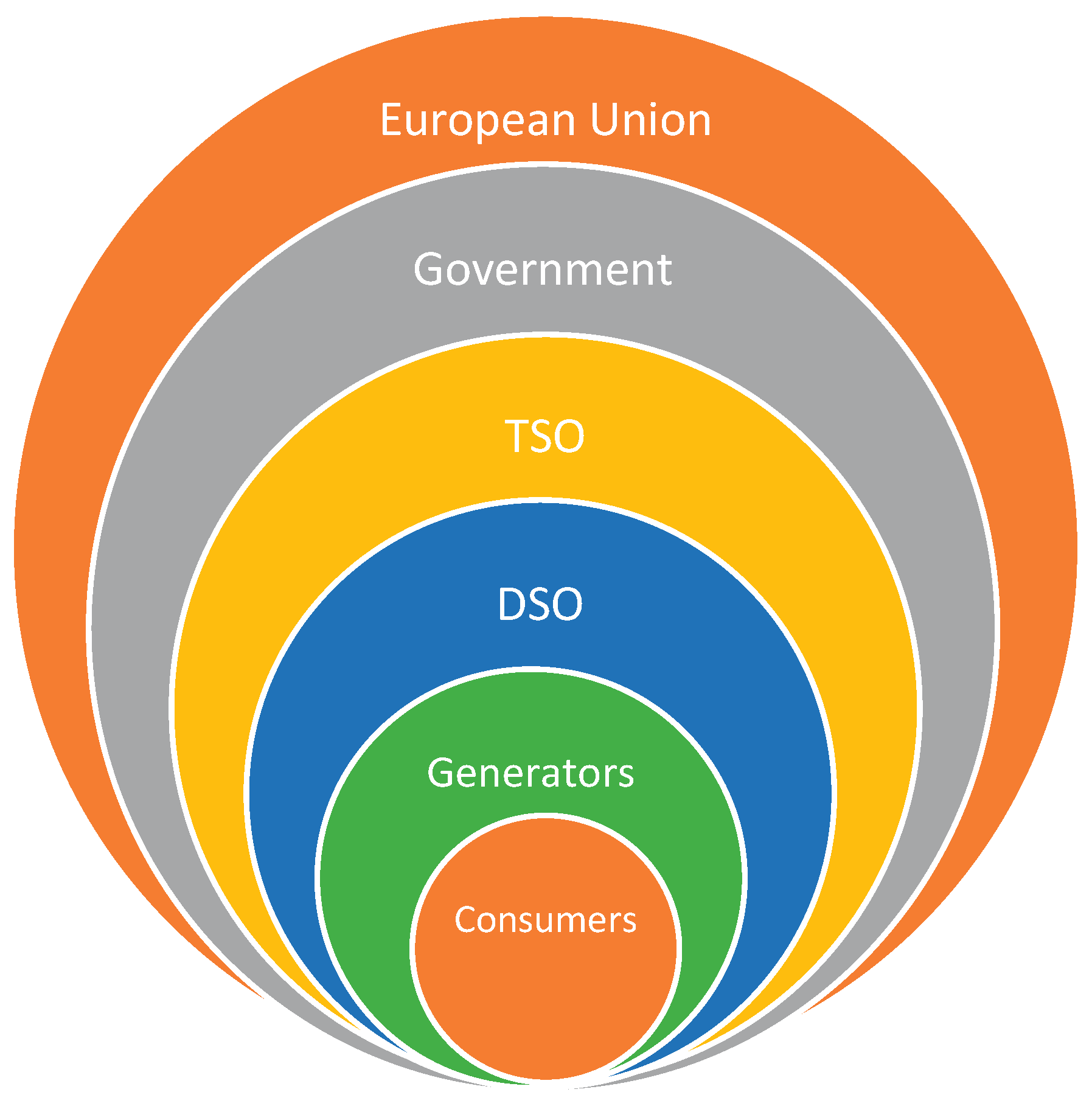
Figure 2.
Development decision-makers and their objectives.
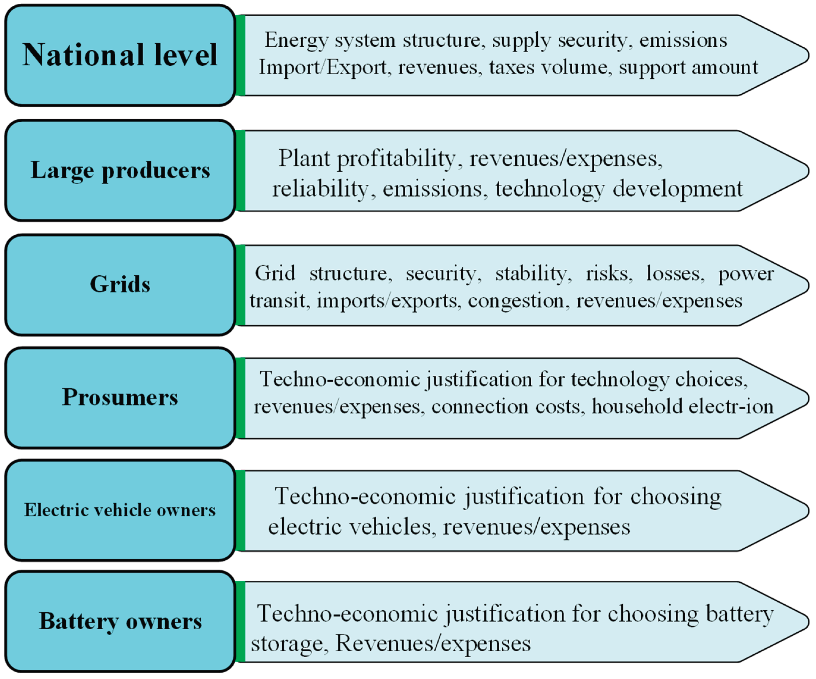
Figure 3.
Block Diagram of the Conventional Power System Planning Approach. FM – Forecasting Module; SG –Scenario Generator; DM – Decision Makers; PSMM – Power System and Market Module; OSD - Objectives, Structures and Decision variables.
Figure 3.
Block Diagram of the Conventional Power System Planning Approach. FM – Forecasting Module; SG –Scenario Generator; DM – Decision Makers; PSMM – Power System and Market Module; OSD - Objectives, Structures and Decision variables.
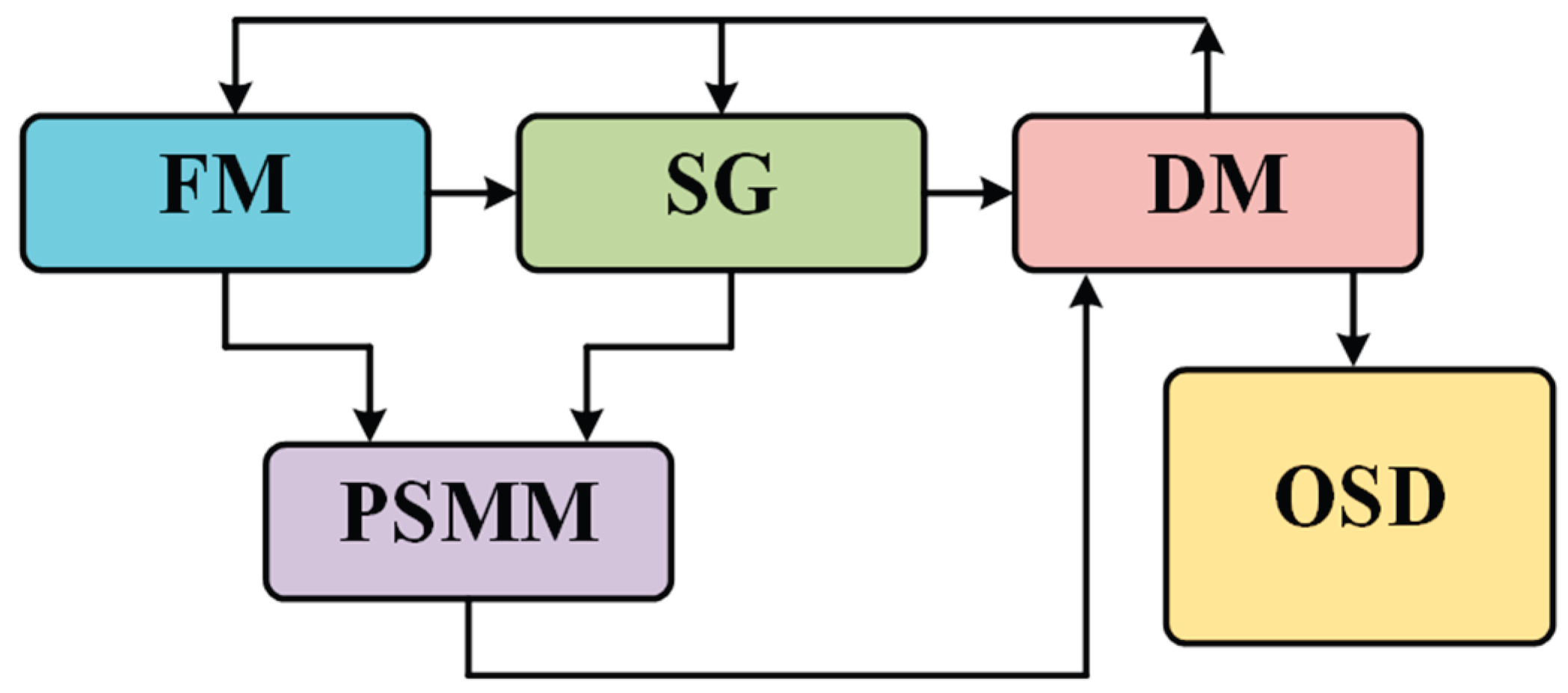
Figure 4.
Block Diagram of the Proposed Power System Planning Approach.
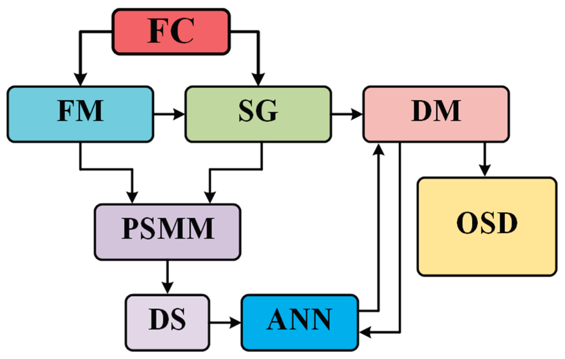
Figure 5.
Structure of the proposed scenario-based surrogate modeling framework.
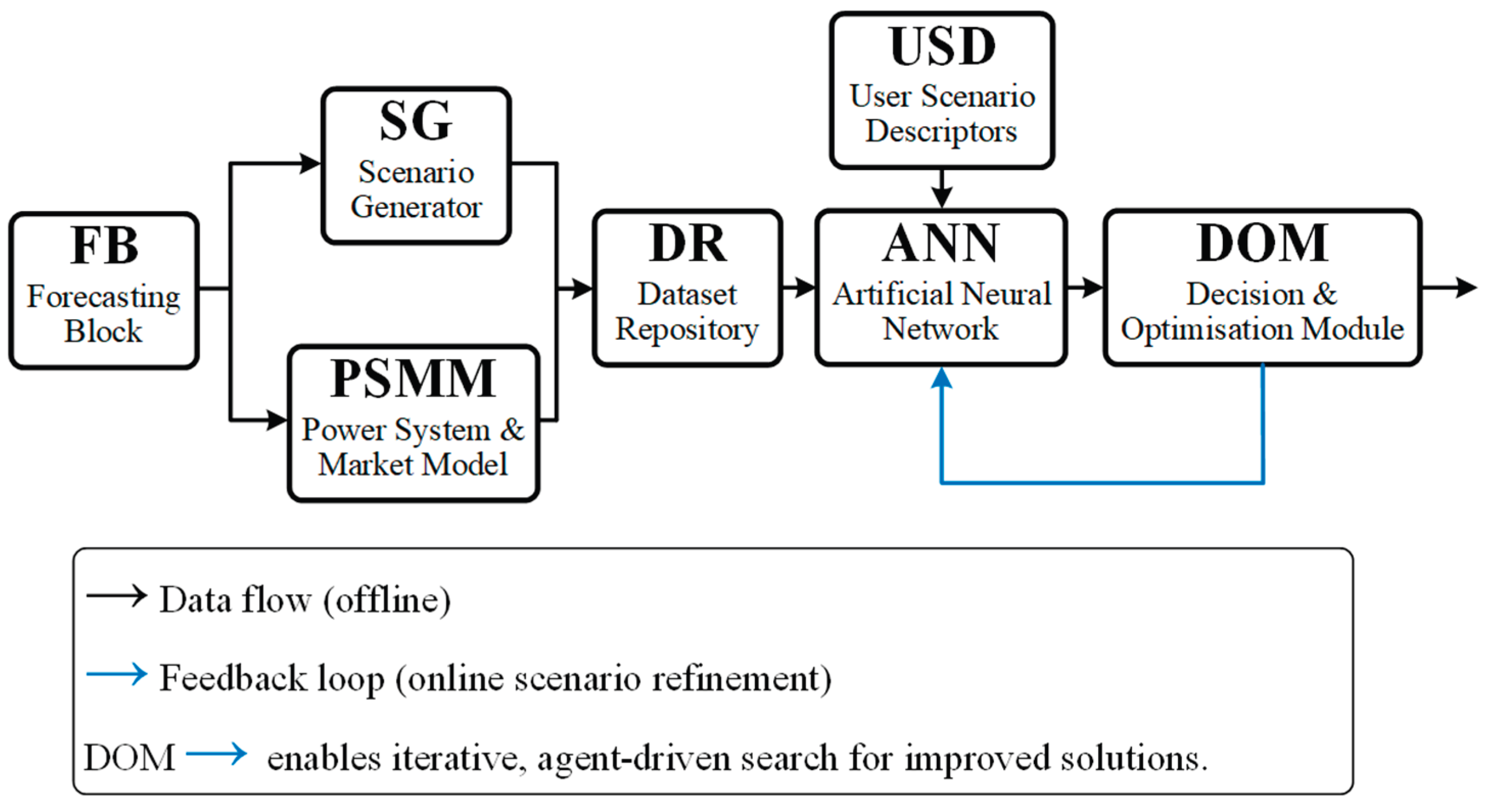
Figure 6.
Variable Decomposition Framework for Long-Term Forecasting.
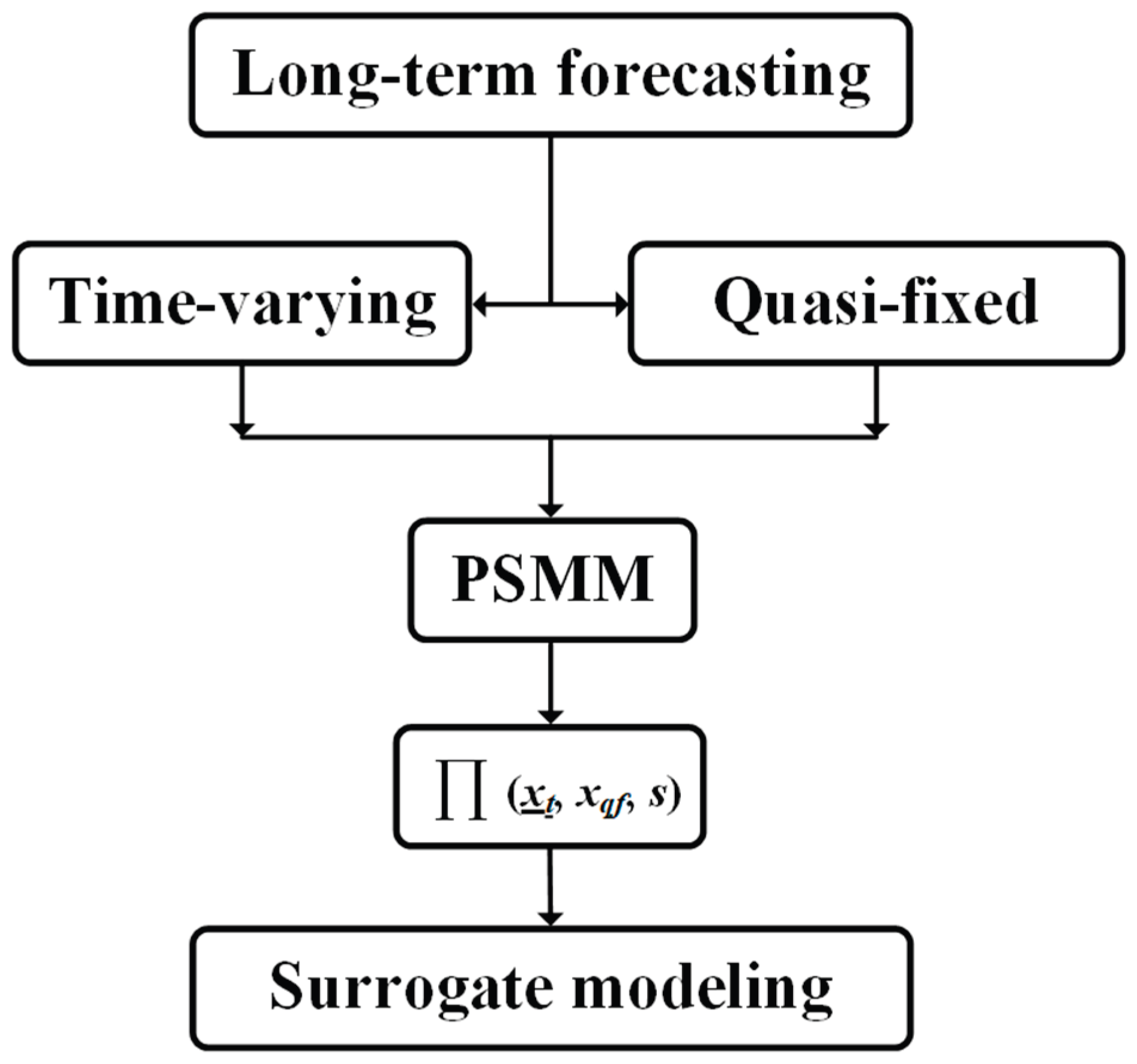
Figure 8.
The structure of energy system model.
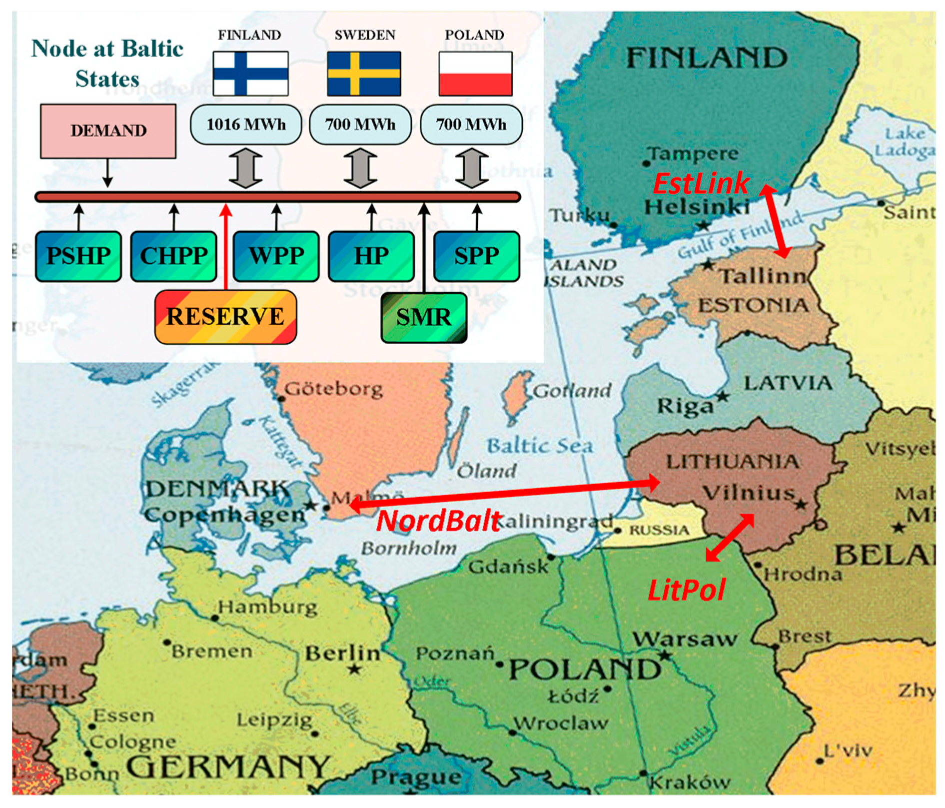
Figure 9.
Centered consumption deviation in the BPS at hourly resolution.
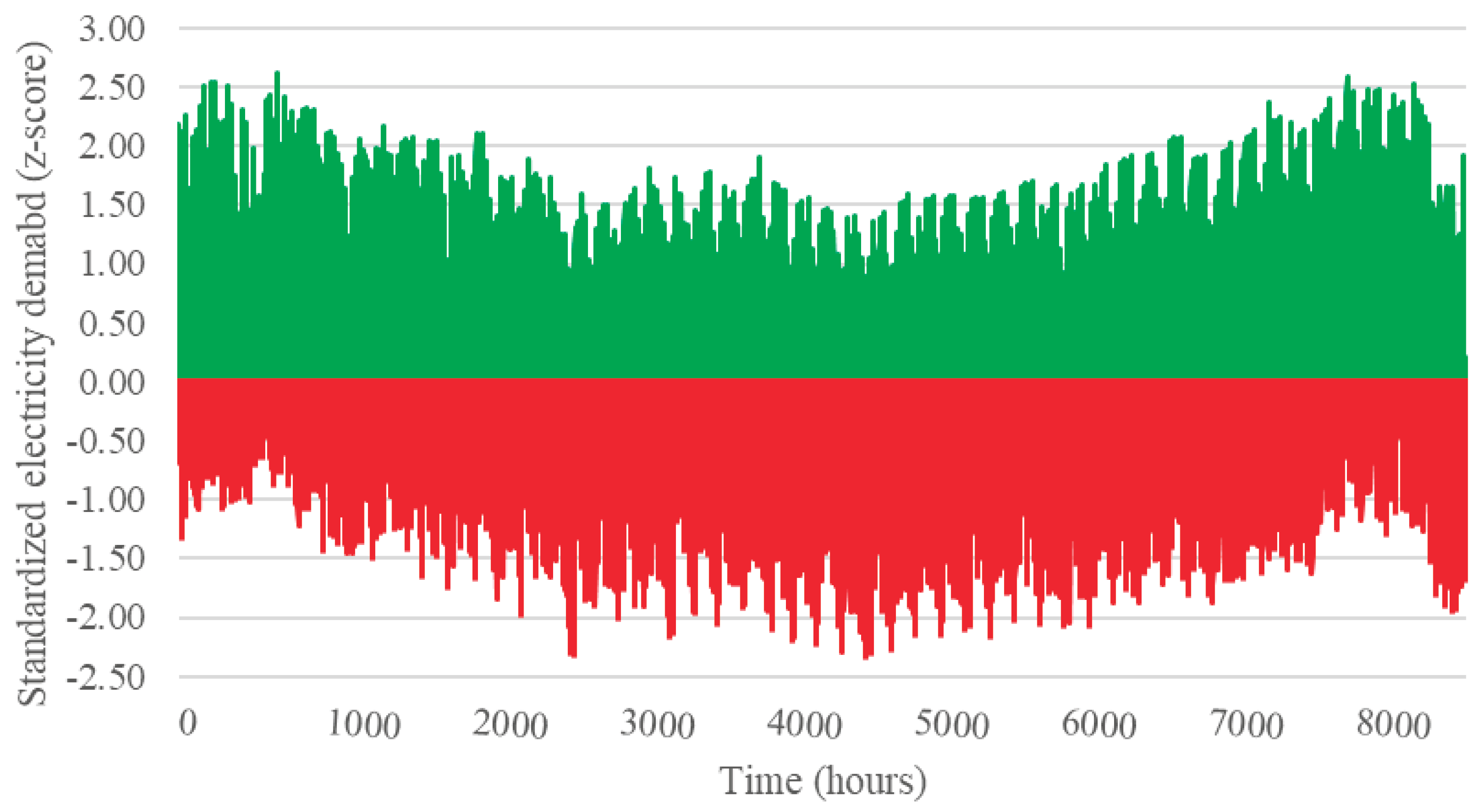
Figure 10.
Centered WES and SES generation in the BPS at hourly resolution.
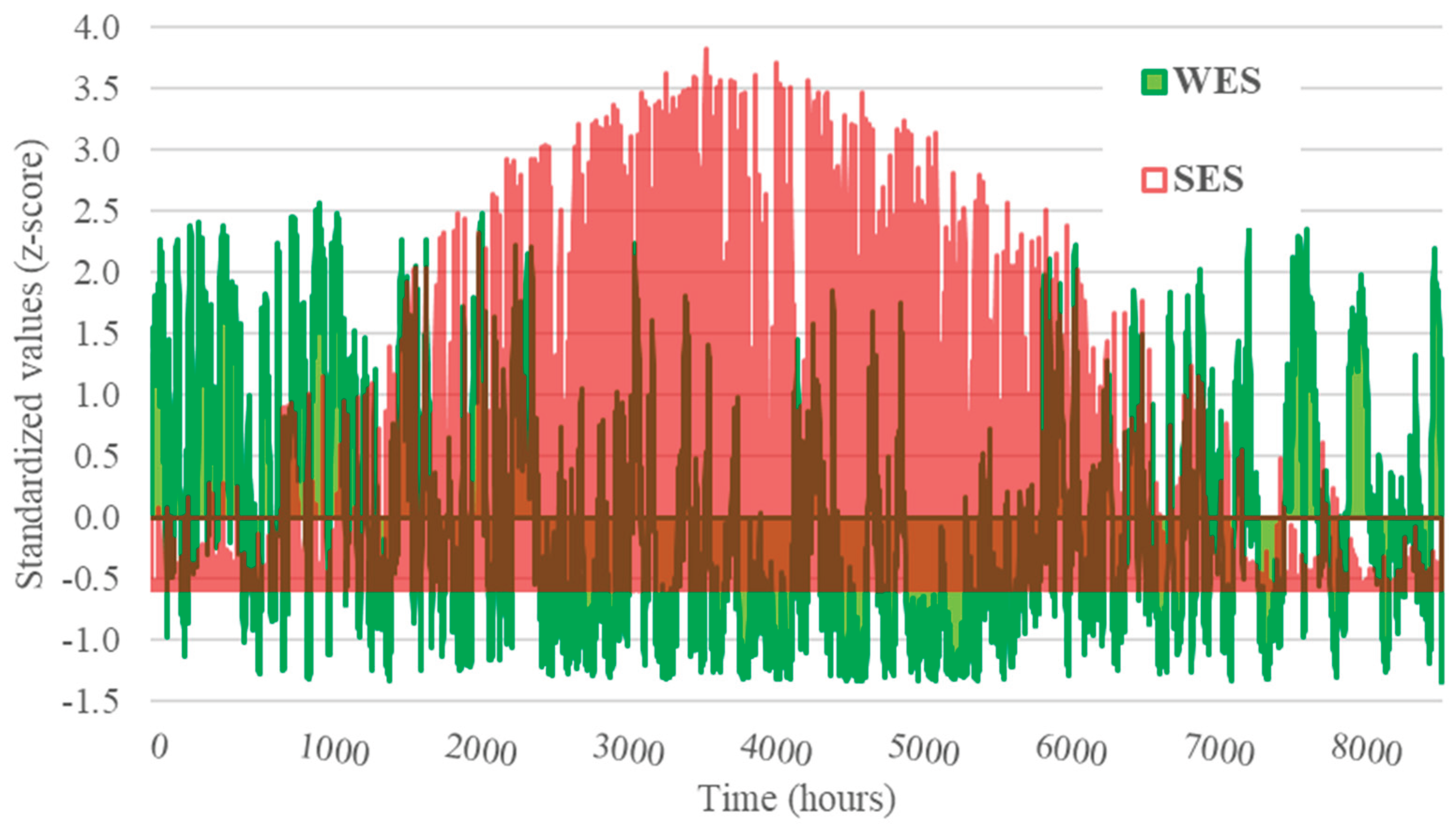
Figure 11.
Subspace of input parameters of the training dataset D.
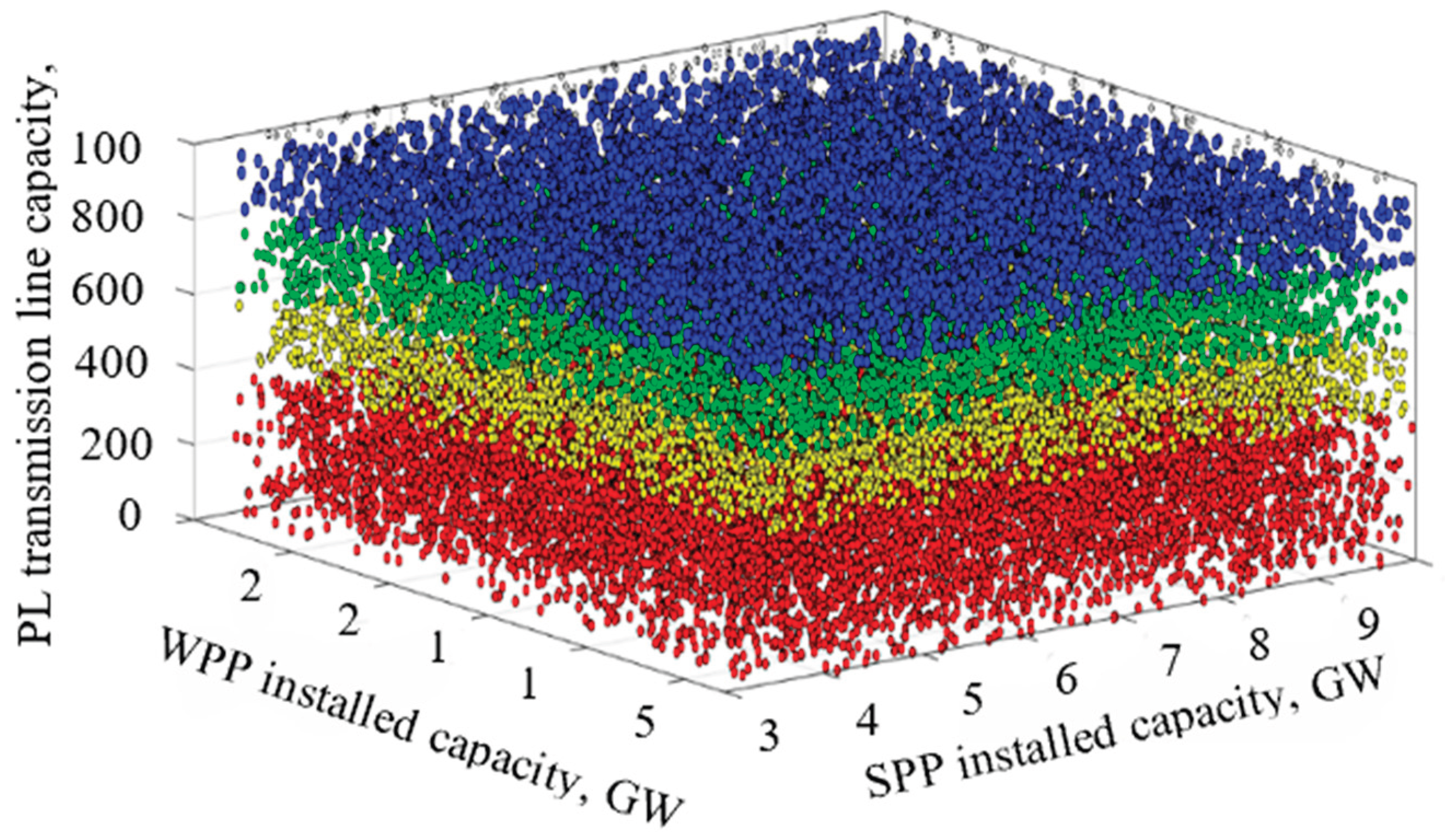
Figure 12.
Annual income and expenditure from exports and imports.
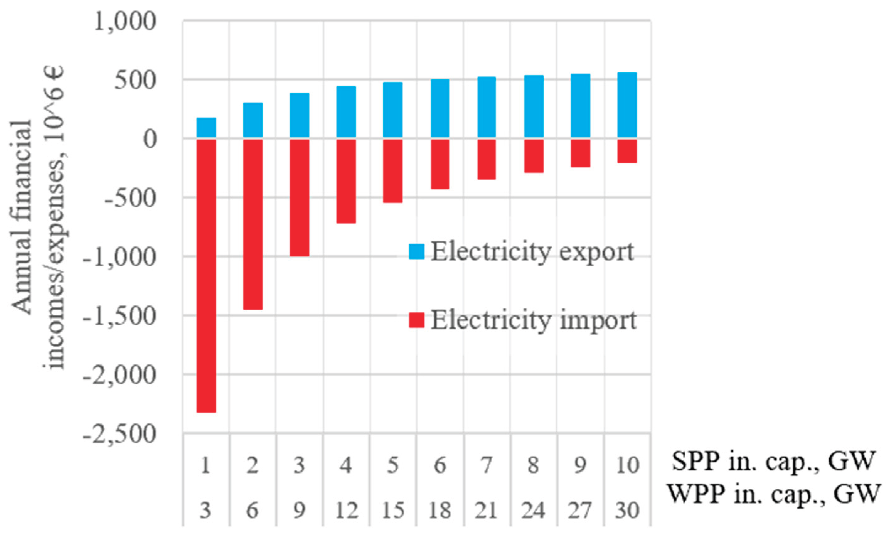
Figure 13.
Annual imports expenditure.
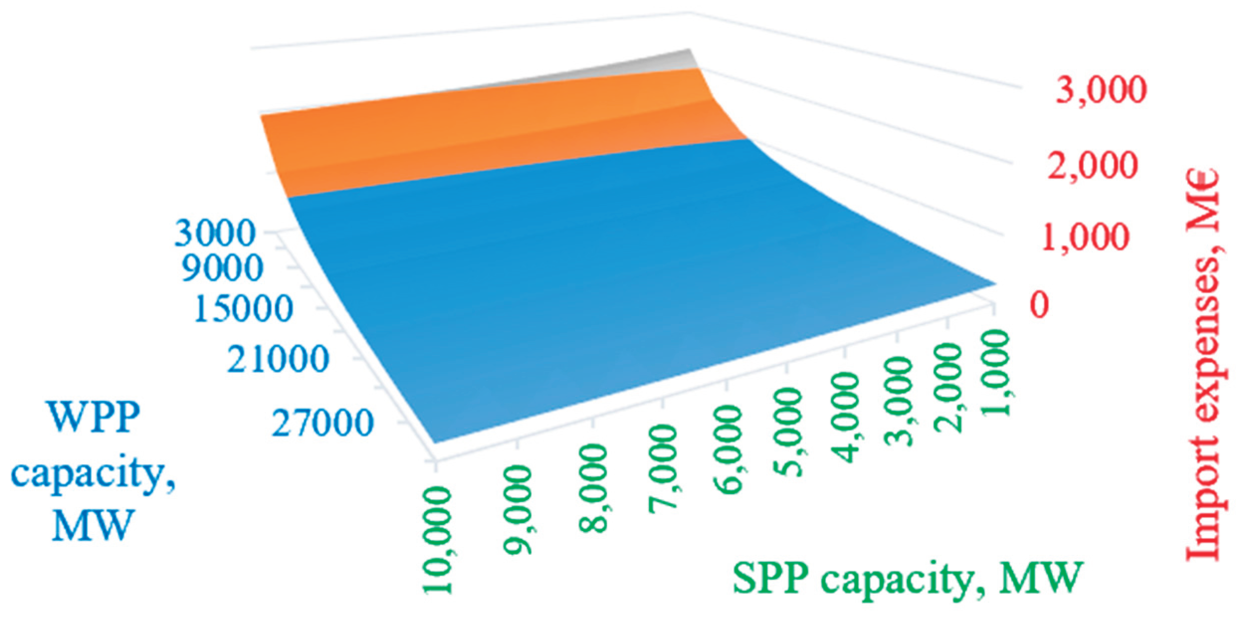
Figure 14.
Relationship between profit and average annual electricity price and the reserve energy price.
Figure 14.
Relationship between profit and average annual electricity price and the reserve energy price.
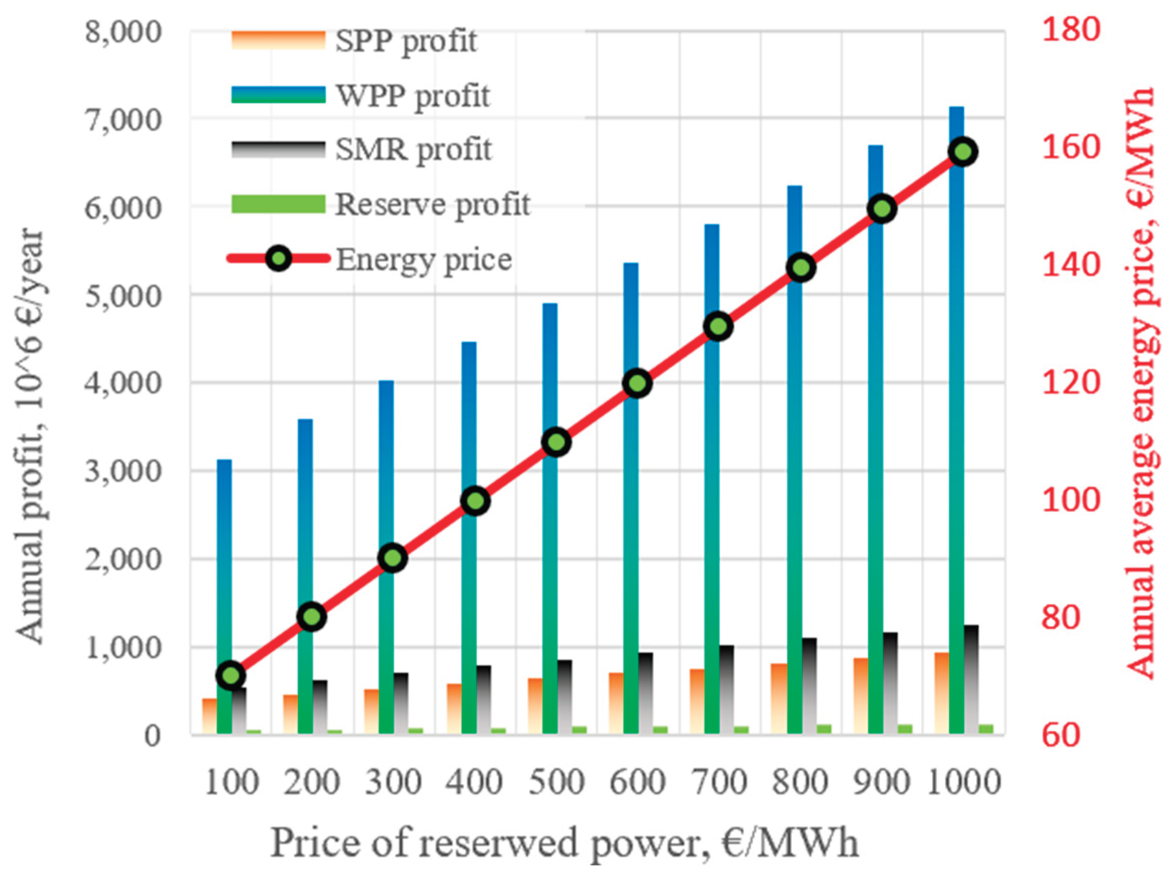
Figure 15.
Accuracy of surrogate model.
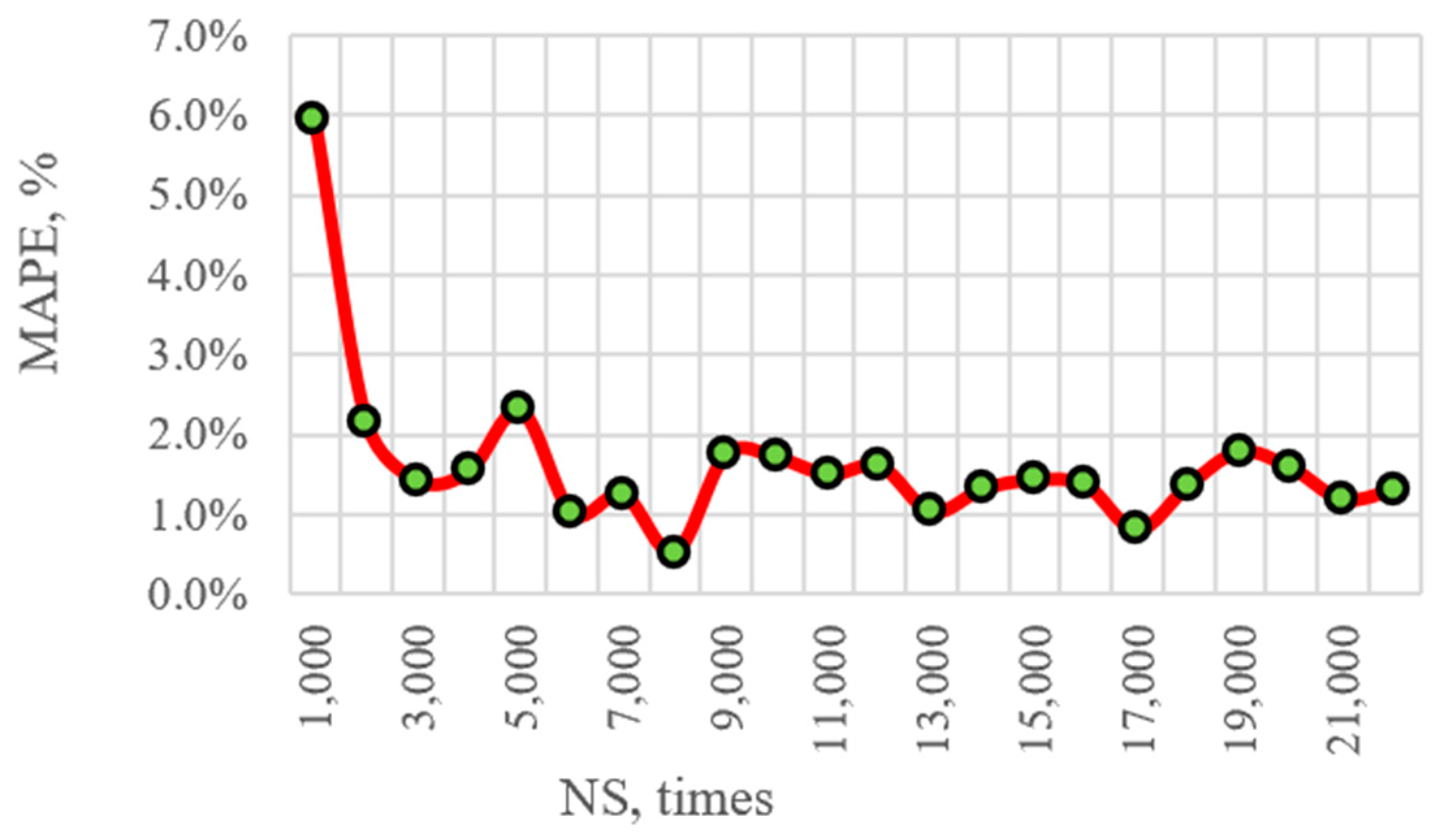
Figure 16.
Error Distribution in Average Market Price Estimation.
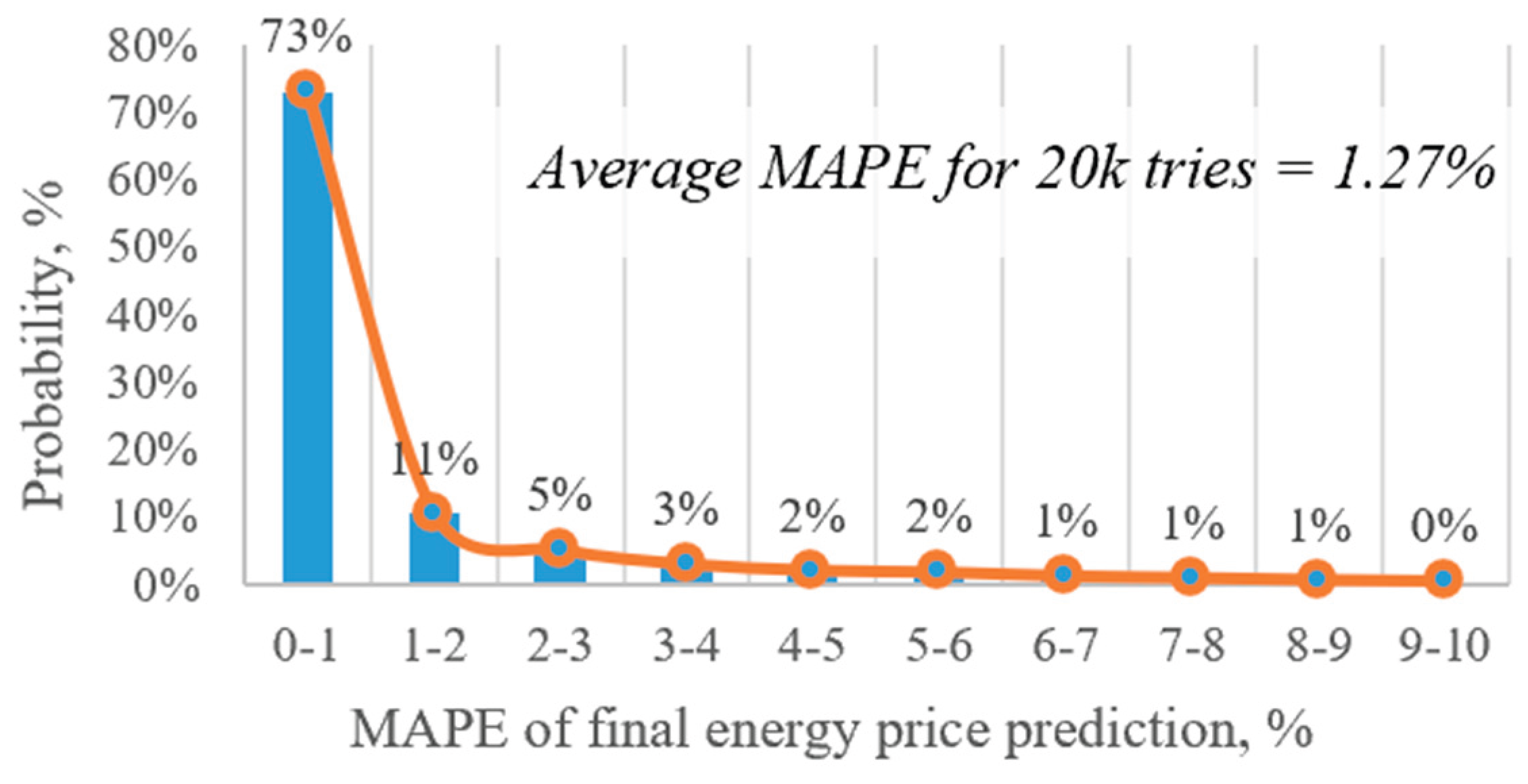

Table 1.
Time-varying (hourly) and quasi-fixed (annual) input variables for scenario generation.
| No | Variable / Process Description | Geographic Scope | Annual Avg (2025) |
Scenarios Range (2025 -2050) Smin/Smax |
Base Scenario | Sources |
| 1 | Solar generation, MWh/h | LV | 120 | 120/5000 | 5000 | [56] |
| 2 | Wind generation, MWh/h | LV | 250 | 250/15000 | 15000 | [56] |
| 3 | Water inflow / hydro, m3/s | LV | 600 | 600/600 | 600 | [61] |
| 4 | SMR* | EE/LV | 900 | 0/1200 | 600 | [62] |
| 5 | BPP**, MW | LV/EE/LT | 522 | 522 | 522 | [56] |
| 6 | PSHP***, MW | LT | 1625 | 1625 | 1625 | [56,63] |
| 7 | Reserve PP****,MW | EE/LV/LT | 1500 | 1500 | 1500 | [57,59] |
| 8 | Electricity demand, TWh/Y | EE/LV/LT | 28 | 28/132 | 43 | [56] |
| 9 | Zonal market prices, EUR/MWh | SE /FI / PL | 32/31/45 | 32/135 31/134 45/195 |
52/51/ 75 | [64] |
| 10 | Reserve PP energy price EUR/MWh | SE /FI / PL | 200 | 100/1000 | 300 | [65] |
* Small Modular Reactor [62]; ** Bio power plants; *** Pumped-Storage hydropower plants; **** Reserve power plants.
Disclaimer/Publisher’s Note: The statements, opinions and data contained in all publications are solely those of the individual author(s) and contributor(s) and not of MDPI and/or the editor(s). MDPI and/or the editor(s) disclaim responsibility for any injury to people or property resulting from any ideas, methods, instructions or products referred to in the content. |
© 2026 by the authors. Licensee MDPI, Basel, Switzerland. This article is an open access article distributed under the terms and conditions of the Creative Commons Attribution (CC BY) license (http://creativecommons.org/licenses/by/4.0/).
Copyright: This open access article is published under a Creative Commons CC BY 4.0 license, which permit the free download, distribution, and reuse, provided that the author and preprint are cited in any reuse.


