

Submitted:
27 May 2026
Posted:
27 May 2026
You are already at the latest version
Abstract
The integration of photovoltaic (PV) and wind turbine (WT) systems into modern power grids demands not only accurate component-level models but also a holistic understanding of their coordinated operation. This review bridges the gap between low-level device physics and high-level system coordination, offering a dual perspective often overlooked in existing surveys that treat generation and management separately. We systematically analyze PV models, from single-diode equivalent circuits to data-driven approaches, and WT models, ranging from aerodynamic and mechanical representations to simplified electrical equivalents suitable for stability studies. Critically, we then shift focus to the system level by examining Energy Management Systems (EMS) that enable hybrid PV–WT coordination. Unlike prior reviews that emphasize either component accuracy or dispatch strategies alone, this paper highlights the emerging synergy between hybrid PV–WT modeling and EMS architectures. By identifying mismatches between model fidelity and EMS requirements, this review maps a pathway towards more integrated hybrid renewable systems. The discussion synthesizes key trade-offs in scalability, uncertainty handling, and real-time feasibility, underscoring that true potential is unlocked only through intelligent integration of component models and control architectures.
Keywords:
photovoltaic modeling
; wind turbine modeling
; hybrid renewable energy systems
; energy management systems
; component-to-system coordination
; power system integration
; renewable energy control strategies
1. Introduction
The global energy landscape is undergoing a profound transformation driven by the need to mitigate climate change, reduce dependence on fossil fuels, and enhance energy access and security [1]. In response, governments worldwide have introduced new regulations and policies aimed at promoting renewable energy sources (RES) technologies, enhancing energy efficiency, and establishing conservation plans alongside supporting legislation. The advantages of renewable energy sources include the use of freely available resources, namely solar and wind, as fuel, together with low operating and maintenance expenses, and the absence of natural resource depletion. Among renewable energy sources, solar and wind power have emerged as the two dominant pillars, accounting for the majority of new generation capacity installed annually worldwide [2]. This growth is underpinned by decades of technological learning and manufacturing scale-up, which have steadily driven down the levelized cost of solar electricity. As shown in Figure 1, the PV costs dropped significantly in last 50 years [3].
Photovoltaic (PV) systems and wind turbines (WTs) offer complementary characteristics: solar irradiance exhibits diurnal and seasonal patterns, while wind availability often peaks during different hours or seasons, making their hybridization particularly attractive for smoothing power output and improving overall system reliability [4]. As a result, hybrid PV–WT installations, ranging from small off-grid microgrids to large utility-scale renewable plants, have become a mainstream solution for modern power systems [5]. These technologies are applied not only in microgrids but also in fields. For instance, long before the widespread grid integration of PV, the technology found one of its first practical applications in water pumping, with pioneering experiments conducted in the Soviet Union during the mid-1960s, and it is still widely used for pumping applications [6,7,8]
Despite the maturity of PV and WT technologies as standalone systems, their effective integration into hybrid configurations poses nontrivial challenges that span multiple temporal and spatial scales [9]. At the component level, accurate modeling is essential for predicting energy yield, designing power converters, and implementing maximum power point tracking (MPPT). The literature on PV modeling is extensive, encompassing equivalent-circuit models (e.g., single-diode, double-diode), empirical models, and more recently, data-driven approaches based on machine learning [10,11]. Similarly, wind turbine modeling spans aerodynamic representations (blade element momentum theory), mechanical drivetrain dynamics, and various generator-converter topologies (fixed-speed, doubly-fed induction generators, permanent magnet synchronous generators) [12,13]. Each model type involves trade-offs among accuracy, computational cost, and parameter availability, choices that have significant downstream consequences.
Based on an analysis of research trends in renewable energy, particularly hybrid PV-wind turbine system simulation, modelling, and optimization, the distribution of papers by major publishers is heavily concentrated among a few key academic publishers.
At the system level, the focus shifts from individual components to coordinated operation. Energy Management Systems (EMS) are responsible for dispatching power among PV arrays, wind turbines, storage units, and loads while satisfying technical constraints, economic objectives, and grid code requirements [14]. EMS strategies range from simple rule-based logic (e.g., state-of-charge thresholds) to advanced optimization methods (e.g., linear programming, model predictive control) and emerging reinforcement learning approaches [15]. Critically, the performance of any EMS depends not only on the control algorithm itself but also on the underlying models used for prediction, state estimation, and constraint formulation. A mismatch between component model fidelity and EMS requirements can lead to suboptimal decisions, instability, or excessive computational burden—a problem rarely addressed in existing reviews.
Existing survey papers tend to fall into three categories. The first focuses exclusively on PV or wind turbine modeling, with little attention to system coordination [16,17]. The second reviews EMS architectures for hybrid renewable systems but treats component models as black boxes, often assuming simplified linear or lookup-table representations without critically examining their limitations [18,19]. The third category addresses hybrid systems from a techno-economic sizing perspective yet again and deemphasizes the dynamic coupling between model choice and control strategy [20]. Consequently, a systematic bridge between component modeling and system coordination is not addressed properly. This gap is increasingly problematic as hybrid systems adopt more sophisticated control methods (e.g., stochastic MPC, learning-based policies) that explicitly rely on model structure and uncertainty characterization.
This review paper directly addresses that gap. We provide a unified examination of PV and WT models alongside EMS architectures, with a specific focus on how model decisions affect coordination outcomes. Our contribution is threefold: (i) a comparative analysis of PV and WT models organized by fidelity, parameter accessibility, and computational suitability for EMS applications; (ii) a structured review of EMS strategies categorized by their underlying model requirements (from model-free to model-based); and (iii) a critical discussion of mismatches, trade-offs, and future directions, including hybrid modeling (physics + machine learning) and real-time coordination under uncertainty.
The remainder of this paper is organized as follows. Section 1 (this section) has introduced motivation and scope. Section 2 reviews photovoltaic models, from equivalent circuits to empirical and data-driven approaches. Section 3 covers wind turbine models, including aerodynamic, mechanical, and electrical representations. Section 4 examines energy management systems at the system level, linking control objectives to model fidelity. Section 5 provides a discussion of key trade-offs, gaps, and future research directions. Section 6 concludes the paper.
2. PV Systems Models
Accurate modeling of photovoltaic systems is fundamental to predicting energy yield, designing power electronics, implementing maximum power point tracking, and evaluating grid integration performance. PV models span a spectrum from simple empirical representations to complex physical equivalent circuits and, more recently, data-driven architectures, Figure 3. The choice of model directly impacts simulation accuracy, computational cost, parameter identification complexity, and ultimately, the effectiveness of higher-level energy management systems that rely on these models for forecasting and optimization. This section provides a structured classification of PV models, organizing them by their underlying principles. Rather than exhaustively cataloging every variant, we focus on model families most relevant to hybrid renewable energy system studies, highlighting their mathematical formulations, key parameters, calibration requirements, and practical limitations in the context of system-level coordination.
2.1. Empirical/Black-Box PV Models
Empirical or black-box models represent photovoltaic systems using purely data-driven relationships without explicit knowledge of internal physical parameters such as diode ideality factors, series resistance, or recombination losses. These models treat the PV system as an unknown nonlinear function that maps inputs (irradiance, temperature, voltage) to outputs (current, power) based solely on measured I-V or P-V data [21]. The primary advantage of empirical models lies in their ability to approximate complex behaviors without requiring detailed physical characterization of the PV cell or module. However, their accuracy is fundamentally limited by the quality, quantity, and representativeness of training data, and they typically lack extrapolation capabilities outside the range of measured conditions.
From an EMS perspective, empirical models offer low computational overhead and rapid evaluation, making them attractive for real-time applications, but their static or quasi-static nature may fail to capture dynamic phenomena such as partial shading transients, bypass diode switching, or thermal hysteresis. Furthermore, black-box models provide no direct insight into physical degradation mechanisms, limiting their long-term reliability for system optimization.
2.1.1. Lookup Table (LUT) Models
Lookup table models pre-store current or power values for discrete combinations of irradiance and temperature, typically derived from manufacturer datasheets or experimental measurements. During operation, the model retrieves the output corresponding to the nearest grid point, often employing linear or bilinear interpolation between entries. The primary appeal of LUT models is their simplicity and deterministic execution time, making them suitable for embedded controllers with limited computational resources.
However, LUT models suffer from several fundamental limitations. First, discretization errors arise from finite table resolution; finer tables reduce error but increase memory requirements and calibration effort. Second, interpolation between points assumes linearity in a fundamentally nonlinear system, leading to systematic inaccuracies near the maximum power point knee region. Third, LUTs cannot adapt to cell aging, soiling, or manufacturing variations without complete recalibration. Fourth, as noted in comparative studies of PV parameter extraction, approximation-based methods (which include LUT approaches) tend to produce incorrect estimation of the simulation current, and the root mean square error (RMSE) compared to more accurate analytical or numerical methods such as the Lambert W or Newton–Raphson approaches [22]. These inaccuracies, while acceptable for rough energy yield estimation, can propagate into EMS optimization errors when used for economic dispatch or battery scheduling.
2.1.2. Polynomial Regression (PR) Models
Polynomial regression models fit low-to-mid-order polynomials to measured I-V or P-V data, expressing output power or current as a polynomial function of irradiance, temperature, and sometimes voltage. These models range from simple univariate quadratic fits to multivariate polynomial surfaces with cross-terms. Regression models were additionally employed to predict solar power output. The following equation represents a basic regression model for PV power [23]:
where:
Pout – is output power, W
G – is the solar irradiance, W/m2
kn – are regression coefficients
Tamb – is the ambient temperature, °C
v – is the air speed at 10m above grade, m/s
The primary advantage of polynomial regression is its analytical tractability: polynomial expressions are differentiable, continuous, and computationally trivial to evaluate—properties that align well with gradient-based optimization methods commonly used in EMS. In [24], authors demonstrated that multivariate polynomial regression could achieve greater accuracy compared to conventional analytical methods for modeling photovoltaic-thermal (PVT) systems, while maintaining minimal model complexity suitable for control applications. Similarly, authors in [25] employed exponential polynomial regression models to forecast daily PV power generation using daylight duration as the primary predictor, achieving a standard residual error of 0.3022 kWh.
Nevertheless, polynomial regression has well-documented drawbacks. High-degree polynomials are prone to Runge's phenomenon (oscillatory behavior at interval boundaries), necessitating careful order selection. Extrapolation beyond the training range is notoriously unreliable, as polynomial tails diverge rapidly. Furthermore, polynomial models assume a fixed functional form that may not capture abrupt changes due to partial shading, cloud edge effects, or bypass diode activation.
2.1.3. Artificial Neural Networks (ANN)
Artificial neural networks represent the most flexible and powerful class of black-box PV models. ANNs learn nonlinear input-output mappings from extensive datasets without requiring an explicit mathematical functional form. Common architectures applied to PV modeling include multilayer perceptron (MLP), recurrent neural networks (RNN), long short-term memory (LSTM), gated recurrent units (GRU), and convolutional neural networks (CNN).
ANNs excel at capturing complex, nonlinear relationships, including temperature-dependent efficiency variations, spectral effects, and partial shading patterns that are difficult to model analytically. In [26], the authors provide a comprehensive state-of-the-art review of five advanced ANN architectures for PV power forecasting, concluding that bidirectional GRU and LSTM offer higher forecasting accuracy, whether used as a standalone model or in a hybrid configuration. They also note that hybrid and upgraded metaheuristic algorithms have demonstrated exceptional performance when applied to standalone and hybrid ANN models.
For PVT systems integrated with phase change materials (PCM), authors in [27] reviewed ANN applications and found that MLPs can achieve high accuracy for stage limits when the models reach a steady situation, while recurrent networks like LSTM explain adequately the dynamic behaviour characteristics of the thermal responses.
However, ANNs carry substantial practical burdens. They require large, high-quality training datasets covering the full operational envelope, including rare events such as extreme temperatures or soiling conditions. Architecture selection (number of layers, neurons, activation functions) remains more art than science, often requiring extensive hyperparameter tuning. Overfitting is a persistent risk, particularly with limited data. Finally, the "black-box" nature of ANNs limits interpretability: it is difficult to diagnose why a model failed or to guarantee physically plausible outputs (e.g., negative power at zero irradiance) without explicit constraints.
From an EMS perspective, the computational demands of ANNs, particularly during training, may be prohibitive for embedded real-time applications, though inference (forward pass) is typically fast.
2.2. Physical/Grey-Box PV Models
Equivalent-circuit models, also referred to as physical or grey-box models, represent the photovoltaic cell as a network of ideal electronic components that mirror the underlying semiconductor physics. Unlike black-box approaches, these models incorporate explicit circuit elements, current sources, diodes, and resistors, each corresponding to a specific physical phenomenon within the cell. The photocurrent source represents electron-hole generation by incident photons, the diodes model the p-n junction behavior, series resistance accounts for bulk and contact resistances, and shunt (parallel) resistance captures leakage currents due to manufacturing imperfections or material impurities.
The primary advantage of equivalent-circuit models lies in their interpretability: each parameter has a physical meaning, enabling diagnosis of degradation mechanisms, prediction of performance under varying conditions, and extrapolation beyond measured data ranges. Furthermore, these grey-box models strike a balance between the complete opacity of black-box methods and the prohibitive complexity of full numerical device physics simulations.
However, the parameter estimation problem for equivalent-circuit models is inherently challenging [28]. As noted in comprehensive surveys, the characteristic equation of the single diode model is transcendental, meaning no closed-form analytical solution directly relates current and voltage without iterative or approximate methods. This mathematical property transforms parameter extraction into a non-convex optimization problem, requiring careful selection of numerical, analytical, or metaheuristic techniques. Moreover, the increased accuracy of more complex models (double-diode, triple-diode) comes at the cost of additional unknown parameters, exacerbating identifiability issues and computational demands.
From an EMS perspective, equivalent-circuit models are preferred for dynamic studies, MPPT design, and grid integration analyses where physical consistency and extrapolation capability are essential. Nevertheless, the computational burden of iterative parameter extraction and the propagation of parameter uncertainty into EMS optimization decisions remain significant practical concerns.
2.2.1. Single-Diode Model (SDM)
The single-diode model is the most widely adopted equivalent-circuit representation in PV literature, offering an optimal compromise between accuracy and complexity. The model consists of five key parameters: photocurrent Iph, diode reverse saturation Isat, diode ideality factor a, series resistance Rs, and shunt resistor Rsh, Figure 4.
The governing equation expresses the output current Io as a function of terminal voltage V0 [29]:
where:
I0 – is the output current, A
Iph – is the light generated current, A
Id – is the diode reverse saturation current, A
q – is electron charge, 1.602 ×10⁻¹⁹ C
a – is ideality factor,
k – is Boltzmann constant, 1.381×10⁻²³ J/K
V0 – is the output voltage, V
T – is the temperature, K
Rs – is the series resistance, Ω
Rsh – is the shunt resistance, Ω
ns – is the number of cells connected in series,
np – is the number of cells connected in parallel
The SDM captures the primary current-voltage characteristics of PV cells with remarkable fidelity across most operating conditions. Its five parameters correspond to distinct physical phenomena: Iph scales linearly with irradiance, Io and a describe recombination in the space-charge region, while Rs and Rsh account for ohmic losses and leakage paths, respectively. The model's popularity stems from its tractable parameter space (only five unknowns) and the availability of numerous extraction methods ranging from analytical approximations to sophisticated metaheuristic algorithms [30].
The SDM is the preferred choice for EMS applications requiring a balance between physical interpretability and computational feasibility. Its five-parameter structure enables temperature and irradiance corrections essential for forecasting and real-time optimization. However, the need for iterative current calculation can become a bottleneck in embedded EMS implementations with stringent timing constraints.
The SDM is widely used in literature, in [31] the authors investigated the PV power supply of a centrifugal pump system with the help of single diode model in Matlab/Simulink (R2018a) environment. The model allows to simulate the properties of a specific PV module (SunPower SPR-415E) with a nominal output power of approximately 400W, Figure 5. The model helps to estimate the energy yield and compare it to the pumping system’s consumption demand.
2.2.2. Double-Diode Model (DDM)
The double-diode model (DDM) extends the SDM by incorporating a second diode in parallel with the first, providing a more accurate representation of recombination phenomena within the solar cell, Figure 6.
The physical justification for the DDM lies in the distinct recombination mechanisms occurring in different regions of the cell. The first diode D1 represents recombination in the bulk neutral regions via the Shockley-Read-Hall mechanism. The second D2 accounts for recombination in the space-charge region (depletion layer) where carrier concentrations are lower [32]. At high irradiance levels (typical operating conditions), the ideality factor for first diode dominates, and the DDM effectively reduces to the SDM. However, at low irradiance, such as dawn, dusk, or cloudy conditions, space-charge recombination becomes proportionally significant, and the DDM achieves superior accuracy.
The DDM's seven-parameter space is considerably more challenging than the SDM's five-parameter problem. The increased dimensionality exacerbates identifiability issues, multiple parameter combinations can produce nearly identical I-V curves, making physical interpretation ambiguous. Furthermore, metaheuristic algorithms often require more iterations and careful hyperparameter tuning to avoid premature convergence to suboptimal solutions [33].
The DDM is most relevant for EMS applications that must operate accurately under variable irradiance conditions, such as microgrids in regions with frequent cloud cover or hybrid systems where PV forecasting during low-light periods is critical. The computational overhead of iterative current calculation or Lambert W function evaluation may, however, limit real-time applicability. Reduced-order approximations of the DDM represent an active research area for embedded EMS deployment.
2.2.3. Tripple-Diode Model (TDM)
The triple-diode model represents the most detailed equivalent-circuit formulation commonly found in the literature, incorporating three parallel diodes to capture recombination phenomena across multiple regions of the PV cell. The physical rationale for the third diode is the modeling of grain boundary effects and additional recombination centers present in polycrystalline and thin-film technologies. While the SDM and DDM were originally developed for monocrystalline silicon cells, emerging PV technologies, including polycrystalline, perovskite, and thin-film, exhibit more complex recombination behavior that may benefit from additional circuit elements.
In [34], the authors proposed a novel, scalable triple-diode based generalized PV model implemented in MATLAB/Simulink. Their model offers the flexibility to represent SDM, DDM, or TDM configurations by including nine or fewer parameters, enabling inclusive comparison across model complexities. Validation against nine commercial PV modules under standard test conditions yielded modeling errors ranging from 0.2% to 7.31%, demonstrating accuracy comparable to or superior to widely referenced practical models. Furthermore, scalability was verified by modeling a 100 kW PV array under hot climatic conditions (Jodhpur, Rajasthan, reaching 50°C ambient temperature), where the model correctly simulated a 13.26% average output power reduction.
A comparative study in [35] evaluated SDM, DDM, and TDM for fitting I-V curves of perovskite solar cells using a hybrid PSO-SQP optimization algorithm. Their results indicate that the TDM exhibited better performance in capturing the I-V characteristics of PSCs with greater precision and fewer iterations, surpassing both the SDM and DDM. However, the authors noted a critical caveat: for all three models, the extracted ideality factors deviated from the conventional range expected for single-junction cells. Constraining ideality factors within this physically plausible range compromised fitting accuracy, suggesting that the physical interpretation of the model parameters that are commonly accepted for single junction semiconductor cells is not applicable for PSCs. This finding underscores a broader concern: increased model complexity does not guarantee physically meaningful parameters, and validation should consider both curve-fitting metrics and parameter plausibility.
The TDM is generally too computationally intensive for real-time EMS applications, given the nine-parameter optimization and iterative current calculation. However, its value lies in offline applications such as technology assessment, degradation studies, and the development of reduced-order models for specific cell types.
2.3. Approximate Models
Approximate PV models deliberately sacrifice a degree of accuracy in exchange for computational speed, analytical tractability, or ease of implementation. These models are particularly valuable in applications where absolute precision is less critical than rapid evaluation, convex optimization guarantees, or minimal parameter requirements. Common use cases include preliminary system sizing, real-time EMS with limited computational resources, educational demonstrations, and optimization problems where the non-linearities of full equivalent-circuit models would render the problem intractable.
The fundamental trade-off across all approximate models is between fidelity and simplicity. While these models may introduce systematic errors, sometimes exceeding 10–15% near the maximum power point, they enable closed-form analytical solutions, reduce simulation time by orders of magnitude, and allow the use of linear programming or quadratic programming techniques that guarantee global optimality [36].
2.3.1. Ideal Current Source (ICS) Model
The ideal current source model represents the simplest possible PV abstraction, neglecting all diodes and resistances [37]. In this model, the PV generator is treated as a current source whose output current depends only on irradiance, remaining constant regardless of terminal voltage until the open-circuit voltage is approached, at which point the current drops abruptly to zero. The short-circuit current scales linearly with irradiance, meaning that at half the standard irradiance, the current is also halved, while the open-circuit voltage is typically assumed constant or only weakly dependent on temperature [38].
This model captures only the most basic PV behavior: current proportional to irradiance, independent of voltage until open circuit [39]:
where:
ILref – is the short circuit current, A
α – is the current-temperature coefficient, A/ °C
TC – is the cell temperature, °C
It completely ignores the exponential diode characteristic, the voltage-dependent current roll-off, and the existence of a maximum power point distinct from the short-circuit and open-circuit conditions. As a result, the model cannot predict power output for any operating point other than short circuit, making it essentially useless for maximum power point tracking or power flow analysis. Despite these limitations, the ideal current source model finds occasional use in extremely high-level system studies where PV is aggregated with other sources and only annual energy yield estimates are required. Some very early microgrid sizing tools employed this model, assuming the PV array always operates at its maximum power point, which the model cannot represent [40]. Contemporary applications are limited to educational contexts or first-order feasibility checks.
The ideal current source model is unsuitable for any EMS application requiring dispatch decisions based on actual PV power availability. Its only possible use is in preliminary system sizing where worst-case or average irradiance conditions suffice, and even then, a simple fixed derating factor applied to nameplate capacity would be more accurate.
2.3.2. Linear Approximation (LA) Model
Linear approximation models replace the nonlinear exponential current-voltage relationship of PV cells with piecewise linear or globally linearized representations. These models are motivated by the desire to embed PV systems into linear programming, quadratic programming, or mixed-integer linear programming EMS formulations, where convexity and linearity guarantees enable efficient solution using commercial solvers such as CPLEX, Gurobi, or open-source alternatives.
The simplest linearization replaces the entire current-voltage curve with a single straight line connecting the short-circuit point (zero voltage, short-circuit current) and the open-circuit point (open-circuit voltage, zero current) [41]. This linear relationship implies a constant negative slope, meaning the PV behaves like a fixed resistor. The corresponding power becomes a quadratic function of voltage, reaching its maximum at exactly half the open-circuit voltage, with maximum power equal to one-quarter of the product of short-circuit current and open-circuit voltage. For typical crystalline silicon cells, where the fill factor ranges from 0.7 to 0.85, this linear approximation overestimates the true maximum power point voltage and underestimates maximum power.
To improve accuracy while retaining linearity, researchers have developed piecewise linear models that partition the current-voltage curve into multiple linear segments [42]. A common approach uses three segments: a shallow-slope region near short circuit, a steep-slope region near the maximum power point, and a near-vertical region approaching open circuit. Each segment is represented by a simple linear equation of the form current equals slope times voltage plus intercept, with each equation valid only within a specific voltage range.
Linear approximation models are valuable for EMS formulations that require convexity or linearity guarantees, such as real-time dispatch using linear programming, unit commitment with PV uncertainty represented via linear chance constraints, and coordinated control of PV-storage systems where quadratic costs are acceptable. However, users must compensate for systematic underestimation of PV power at the maximum power point, typically by scaling the linear model or incorporating a correction factor derived from offline simulation.
2.3.3. Fractional Open-Circuit Voltage (FOCV) Model
The fractional open-circuit voltage method is one of the simplest and most widely implemented approaches for maximum power point tracking in small-scale PV systems [43]. Rather than modeling the full current-voltage curve, this method exploits an empirical observation: for most PV technologies, the maximum power point voltage is approximately a fixed fraction of the open-circuit voltage across a wide range of operating conditions. This fraction, typically denoted as k, generally ranges from 0.71 to 0.80 depending on cell technology. For crystalline silicon cells, the commonly cited value is approximately 0.76, while for thin-film technologies such as amorphous silicon or CIGS, the fraction may be lower, typically between 0.70 and 0.75, due to different recombination characteristics [44].
In practical implementation, the fractional open-circuit voltage method operates as follows. First, the system periodically disconnects the PV array from the load or briefly opens the circuit. Second, it measures the open-circuit voltage, which requires only a simple voltage measurement and no current sensing. Third, it calculates the target maximum power point voltage by multiplying the measured open-circuit voltage by the fixed fraction k. Fourth, it adjusts the power converter duty cycle to regulate the PV voltage at this calculated target. Finally, it resumes normal operation until the next sampling interval.
The primary advantage of the fractional open-circuit voltage method is its extreme simplicity: no current sensor is required, the control law involves only a single multiplication, and convergence is instantaneous because there is no perturbation or iteration. This makes the method particularly attractive for very low-cost microcontrollers, energy harvesting applications, and systems where the power loss during periodic open-circuit voltage measurement is acceptable.
The fractional open-circuit voltage method is unsuitable as a PV model for EMS applications because it does not provide a continuous power-versus-voltage relationship needed for dispatch optimization. Instead, it is a control technique for local maximum power point tracking. In hierarchical EMS architectures, the local maximum power point tracking controller implementing this method reports available power to the supervisory EMS as a scalar value, which the EMS treats as a parameter rather than as a variable.
2.4. PV Simulation Tools
Beyond component-level mathematical modeling, practical implementation of PV systems for planning, sizing, and energy yield assessment requires specialized simulation tools. These software platforms translate the physical and empirical models described in Section 2.1 through 2.3 into user-friendly interfaces that enable engineers, researchers, and system designers to predict energy production and optimize system configurations [45]. The choice of simulation tool significantly impacts design outcomes, as different software packages employ varying algorithms for irradiance transposition, temperature modeling, shading analysis, and inverter efficiency calculations.
2.4.1. MATLAB/Simulink
In scientific literature, MATLAB/Simulink is the prevailing simulation tool because it is a high-fidelity, equation-based simulation environment widely used for research and development of PV systems, particularly for MPPT algorithm design, power electronics integration, and dynamic system studies [46]. The software includes a built-in PV Array block within the Simscape Electrical toolbox and supports custom implementation of single-diode and double-diode models. For hybrid renewable energy systems, MATLAB/Simulink enables co-simulation of PV arrays alongside wind turbines, battery storage, and grid interfaces, making it a preferred platform for academic research.
2.4.2. PV*SOL
PV*SOL is a professional system-based simulation tool for detailed design and financial analysis of grid-connected PV systems, including building-integrated and off-grid configurations. It distinguishes itself through advanced 3D shading analysis capabilities, enabling accurate modeling of complex rooftop installations with nearby obstructions. The authors in [47] conducted comparative validation study and found that PV*SOL exhibited the lowest error among seven software tools when validated against real-world data from an 84.5 kW solar plant.
2.4.3. Helioscope
A web-based simulation platform Helioscope has a cloud-native PV design known for its intuitive user interface and rapid 3D modeling capabilities. The platform excels at detailed shade analysis using 3D scene reconstruction and supports both fixed-tilt and single-axis tracking systems. Helioscope is particularly popular among commercial solar installers and project developers due to its rapid simulation turnaround time and professional report generation [48].
2.4.4. Solarius PV
A comprehensive system-based simulation tool Solarius PV is offering integrated design, shading analysis, and financial reporting for residential, commercial, and utility-scale PV systems. The tool features a built-in 3D modeling environment for accurate shading assessment and supports a wide range of module and inverter databases [49]. In validation studies, Solarius PV demonstrates among the lowest errors compared to real-world performance data, indicating high credibility for accurate energy yield prediction.
2.4.5. HOMER Pro
A specialized simulation and optimization tool HOMER Pro is optimized for hybrid renewable energy systems, including PV-wind-diesel-battery configurations, with a strong focus on techno-economic analysis for off-grid and grid-connected applications [50]. The software performs thousands of iterative simulations across different system configurations to identify the least-cost combination meeting specified reliability constraints. The main feature is that HOMER Pro uniquely bridges component modeling and system-level EMS design, making it particularly relevant for hybrid PV-wind system studies.
2.4.6. SolarGis
A simulation tool, SolarGis, specializes in solar resource assessment and PV performance modeling. It is distinguished by its high-resolution satellite-derived irradiance database [51]. The platform's core strength lies in its long-term time series of global horizontal, direct normal, and diffuse horizontal irradiance, derived from geostationary satellite observations. Solargis is widely used by project developers and financiers for bankable energy yield reports, often in conjunction with other detailed simulation tools.
An overview of the mentioned simulation tools for photovoltaic systems is presented in Table 1.
3. Wind Turbine Models
Wind turbine modeling presents fundamentally different challenges than photovoltaic systems, primarily due to the conversion of mechanical energy from moving air into electrical energy through rotating machinery. Unlike PV cells, which have no moving parts and respond almost instantaneously to irradiance changes, wind turbines exhibit complex multi-physics dynamics spanning aerodynamic forces and electrical generator characteristics across timescales from milliseconds to seconds. These dynamics are further complicated by the stochastic and spatially distributed nature of wind resources, including turbulence, shear, wake effects, and gusts [52]. Consequently, wind turbine models span a broad spectrum from highly detailed aerodynamic simulations to simplified lookup-table or constant power models.
The choice of wind turbine model fidelity has profound implications for simulation accuracy and computational cost. Overly detailed models may be computationally prohibitive for optimization, while overly simplified models may fail to capture critical phenomena such as wake-induced power deficits in wind farms. This section provides a focused classification of essential wind turbine models, Figure 7.
3.1. Power Capture Models
Aerodynamic models describe how a wind turbine extracts kinetic energy from the moving air mass and converts it into mechanical torque on the rotor shaft. This conversion process is governed by the fundamental physics of fluid flow around the turbine blades, and the accuracy of the aerodynamic model directly determines the fidelity of the entire wind turbine representation.
The fundamental equation governing wind turbine power capture expresses the electrical power output as a function of wind speed, turbine geometry, and efficiency factors. The electrical power extracted by a wind turbine is given by the product of the available kinetic power in the wind and two efficiency terms: the aerodynamic power coefficient and the generator efficiency. This relationship is captured by the well-known wind turbine power equation [53]:
where:
PWT – is the wind turbine, W
ρ – is the air density, kg/m3
AWT – is the wind turbine rotor’s swept area with radius R, m2
V3 – is the wind speed, m/s
CWT – is the power coefficient that represents the turbine's aerodynamic efficiency,
ηg – is the efficiency of a generator coupled to WT’s shaft directly or through a step-up gearbox
This fundamental equation forms the basis for nearly all wind turbine models used in power system analysis and EMS applications, from the most detailed aerodynamic simulations to the simplest constant power approximations. Among the two most relevant aerodynamic modeling approaches are the blade element momentum theory and the simplified power coefficient lookup tables. Blade element momentum theory represents the highest fidelity among these, combining momentum conservation principles with local airfoil aerodynamics to predict the power coefficient from first principles without relying on precomputed lookup tables. Simplified power coefficient lookup tables, which store precomputed values of CWT as a function of tip-speed ratio and blade pitch angle, are the most common choice for EMS applications because they evaluate the complete power equation in a single table lookup, avoiding iterative calculations.
3.1.1. Blade Element Momentum (BEM)
Blade element momentum theory is the industry-standard aerodynamic model for wind turbine design and performance analysis, balancing reasonable computational cost with sufficient physical accuracy. The theory combines two complementary approaches: momentum theory, which considers the overall momentum balance of the air flowing through the rotor disk, and blade element theory, which considers the local lift and drag forces on individual blade segments [54]. By solving these two formulations iteratively until convergence, blade element momentum theory predicts the axial and tangential induction factors, from which the power capture and thrust force can be calculated [55].
The key challenge in blade element momentum theory is that the momentum and blade element components are coupled through the induction factors, which are not known a priori. The theory therefore, requires an iterative solution procedure: the induction factors are guessed initially, the blade element calculations are performed, the resulting forces are used to update the induction factors via the momentum equations, and the process repeats until the induction factors stabilize. Under certain operating conditions, such as turbulent wake or heavily loaded rotor states, the standard momentum equations become invalid, and empirical corrections must be applied to ensure convergence. In [56], authors combine the BEM method with PGD to optimize the blade profile of a horizontal axis wind turbine, achieving a 21.7% improvement in the power coefficient for the turbine compared to a 20 kW reference baseline.
3.1.2. Simplified Power Coefficient (SPC) Lookup Table
The simplified power coefficient lookup table model represents the most common and practical aerodynamic model for many applications. Rather than solving the iterative blade element momentum equations online or performing computationally expensive computational fluid dynamics simulations, this model precomputes the power coefficient CWT for a range of operating conditions and stores the results in a lookup table [57]. The tip-speed ratio is defined as the ratio of the blade tip speed to the wind speed. The blade tip speed is the product of the rotor rotational speed and the blade radius. A low tip-speed ratio indicates that the rotor is turning slowly relative to the wind, while a high tip-speed ratio indicates fast rotation. The power coefficient CWT is a strong function of this tip-speed ratio, typically rising from zero at standstill to a maximum at an optimal tip-speed ratio, then gradually decreasing as the rotor spins too fast and encounters increased drag. For modern three-bladed horizontal-axis wind turbines, the optimal tip-speed ratio typically falls between 6 and 8, where the power coefficient reaches its maximum value of 0.45 to 0.50 [58].
The blade pitch angle is the angle between the blade chord line and the plane of rotation. Most large wind turbines employ active pitch control, where the blades can be rotated about their longitudinal axis to adjust aerodynamic forces. In [59,60], the authors propose a two-stage power stabilization control framework for floating offshore wind turbines that integrates field data fusion forecasting with adaptive pitch regulation to mitigate wind-wave coupling perturbations, achieving a 95% reduction in wind power ramp events and a 43.6% reduction in power slope variability.
At wind speeds below rated, the blades are typically set to a fine pitch angle, often zero degrees, to maximize power capture. At wind speeds above rated, the blades are pitched toward feather, reducing the angle of attack and deliberately spilling excess aerodynamic power to prevent generator overload. The power coefficient lookup table therefore, becomes a two-dimensional array, with tip-speed ratio as one dimension and blade pitch angle as the other.
The primary advantage of the lookup table model is its computational efficiency [61,62]. Evaluating the fundamental power equation with a table lookup requires only a few microprocessor operations and can be executed in microseconds, making it suitable for real-time EMS optimization involving hundreds of turbines. Additionally, the model retains physical interpretability because it is directly derived from blade element momentum theory and respects the fundamental physics captured in the power equation. The lookup table also naturally handles the nonlinear relationship between wind speed and power, including the cut-in, rated, and cut-out regions of the turbine operating curve.
3.2. Reduced Order Models
Simplified and reduced-order wind turbine models deliberately sacrifice aerodynamic and mechanical detail to achieve computational speed, analytical tractability, and low parameters. While the full aerodynamic models described in Section 3.1 are essential for turbine design and detailed simulation studies, they are generally too computationally intensive to embed directly within EMS optimization loops that must solve dispatch problems in seconds or minutes [63]. Simplified models bridge this gap by representing the wind turbine as a static or quasi-static power source whose output depends primarily on wind speed, with all internal dynamics, including blade pitch response, generator transients, and drivetrain oscillations, either neglected or aggregated into simple empirical relationships [64].
3.2.1. Constant Power (CP) Model
The constant power model is one of the simplest possible representations of a wind turbine, treating the turbine as a dispatchable power source with a fixed maximum power output. In this model, the wind turbine is assumed to be capable of delivering constant power PWT, up to its rated capacity, whenever wind conditions permit [65]. The control system receives either a forecasted time series of expected power output for day-ahead scheduling or a real-time measurement for intra-day dispatch, and the underlying wind speed, aerodynamic efficiency, and generator dynamics are entirely abstracted away.
The primary justification for the constant power model is that modern wind turbines with fast pitch control and power electronics can regulate their output to a commanded setpoint with high accuracy and rapid response [66]. From the perspective of an EMS operating on minute-to-hour timescales, the wind turbine appears as a controllable power source that can track a dispatch signal, subject to the constraint that the requested power cannot exceed the instantaneous available power determined by wind conditions. Many grid codes now require wind farms to provide dispatchable power, meaning they must be able to curtail output to a specified level below the available power [67].
The limitations of the constant power model become apparent in several scenarios. First, during above-rated wind speeds, the turbine's pitch control system actively limits power to the rated value, and the constant power model correctly captures this behavior. However, during below-rated operation, the available power varies with the cube of wind speed according to Equation (4), and a constant power assumption would be grossly inaccurate if the forecast error is large. Second, the model ignores the turbine's inertial response, which can provide temporary power support during frequency disturbances, a capability increasingly valued by grid operators. Third, the constant power model cannot represent the reactive power capability of modern wind turbines, which can provide voltage support even when active power is curtailed. Fourth, the model assumes perfect tracking of the dispatch signal, whereas real turbines have ramping limits and minimum power thresholds [68].
3.2.2. Linearized Small-Signal (LSS) Model
The linearized small-signal model represents a wind turbine as a linear transfer function relating small perturbations in wind speed to small perturbations in power output around a nominal operating point. This model is derived by taking the first-order Taylor series expansion of the nonlinear power equation around a specific operating condition, such as a particular wind speed, rotor speed, and pitch angle [69]. The resulting linear model captures the local dynamic response of the turbine to small disturbances, such as wind gusts or grid frequency deviations, and is widely used in stability studies and control system design.
The LSS model reveals several important dynamic properties of wind turbines. First, the model includes the inertial response, which describes how the turbine's rotating mass provides temporary power support during frequency disturbances. This inertial response appears as a lead-lag transfer function that can be tuned by the generator controller [70]. Second, the model captures the pitch actuator dynamics, which limit how quickly the turbine can reduce power during above-rated wind conditions. Third, the model includes the drivetrain torsional modes, which are lightly damped oscillations that can affect power quality and mechanical loads.
The linearized small-signal model is primarily relevant for studies that require assessment of wind turbine contribution to grid frequency response or small-signal stability. For example, when a hybrid PV-wind system operates in islanded mode [71], the linearized models of all generators can be combined to analyze the overall system's stability margin and design appropriate controllers. However, for routine dispatch optimization and scheduling, the linearized model is unnecessarily complex, and the simpler lookup table or constant power models are preferred.
3.3. Software Tools for Wind Turbine Simulation
Wind turbine simulation tools span a wide spectrum from flexible equation-based environments for control design to high-fidelity aerodynamic solvers and dedicated controller frameworks. Unlike PV simulation tools that focus primarily on energy yield prediction, wind turbine software must address the multi-physics nature of rotating machinery, including aerodynamics, structural dynamics, and control systems. This subsection reviews four essential software tools often used in the literature for wind turbine simulation: MATLAB/Simulink, OpenFAST, AMR-Wind, and ROSCO.
3.3.1. MATLAB/Simulink
Like for PV systems, this simulation environment is widely used for wind turbine control system design, power converter modeling, and grid integration studies [72]. The software includes specialized blocks for simplified generator modeling, enabling maximum power point tracking implementation and grid synchronization studies without the computational burden of detailed aerodynamic models. For educational and research applications, Simulink models support both induction and synchronous generators, advanced control strategies, and scalable architectures for various wind farm sizes [73]. Its primary limitation is the lack of native high-fidelity aerodynamic models, requiring users to implement custom blade element momentum formulations or couple with external tools.
3.3.2. OpenFAST (FAST)
The industry-standard open-source wind turbine simulation tool OpenFAST is developed by the U.S. National Renewable Energy Laboratory (NREL). It builds upon the legacy FAST v8 code, integrating aerodynamics, hydrodynamics, control systems, and structural dynamics to enable comprehensive coupled nonlinear aero-hydro-servo-elastic time-domain simulations of wind turbines [74]. OpenFAST supports various configurations, including land-based, fixed-bottom offshore, and floating offshore turbines, and is widely used for reference turbine designs such as the IEA 3.4 MW, 10 MW, 15 MW, and 22 MW models. The platform fosters an open-source developer community with robust software engineering, unit testing, and multi-platform build capabilities, making it the foundation for most wind turbine research and development workflows.
3.3.3. AMR-Wind
This tool is a high-fidelity computational fluid dynamics solver developed by NREL for modeling wind farm aerodynamics and atmospheric boundary layer interactions. The solver features adaptive mesh refinement (AMR) capabilities, enabling blade-resolved simulations of wind turbines with unprecedented detail while managing computational cost through dynamic mesh refinement [75]. AMR-Wind is a core component of the ExaWind software stack, which couples it with Nalu-Wind (near-body flow solver), TIOGA (overset grid assembly), and OpenFAST (structural dynamics) to enable large-scale simulations of entire wind farms with blade-resolved turbines [76]. The solver is designed for high-performance computing environments, with simulations scaling to hundreds of millions of cells on GPU-accelerated supercomputers.
3.3.4. Reference Open Source Controller (ROSCO)
ROSCO is NREL's reference controller framework that facilitates the design and implementation of wind turbine and wind farm controllers for fixed and floating offshore turbines. The framework includes a large set of modular controllers and advanced functionalities, including yaw control, individual blade pitch control, and floating platform feedback, that can be combined based on the intended application [77]. ROSCO integrates directly with OpenFAST, enabling representative dynamic simulations with controller models, and supports a Python-based toolbox that allows generic controller tuning without requiring aeroelastic simulations or linearized state-space models [78]. The framework has been used to provide reference controllers for many recent reference turbines, including the IEA 3.4 MW, 10 MW, 15 MW, and 22 MW designs, enabling comparison of controller capabilities across different turbine models.
An overview of the described simulation tools for wind turbines and their advantages is presented in Table 2.
4. Energy Management System for Hybrid PV–WT
While previous Section 2 and Section 3 were focused on component-level models for PV arrays and wind turbines, this section shifts attention to the system level, where energy management systems coordinate multiple generators, storage devices, and loads to achieve reliable, economical, and sustainable operation [79]. An EMS is the decision-making core of a hybrid renewable energy system, responsible for dispatching power among available sources, managing energy storage, scheduling grid interactions, and responding to forecast uncertainties [80]. The performance of any EMS is fundamentally constrained by the fidelity and structure of the underlying component models: a highly simplified constant power PV model enables fast linear programming but cannot capture voltage-dependent curtailment, while a detailed single-diode model provides physical accuracy at the cost of solving nonlinear equations that may be prohibitive in real-time optimization scenarios. EMS architecture can be organized into three broad categories:
- Rule-based;
- Optimization-based;
- Learning-based.
It is important to keep in mind that mismatches between EMS requirements and component model fidelity lead to suboptimal outcomes: overly simple models may cause constraint violations or missed economic opportunities, while overly complex models may render the EMS computationally intractable for real-time deployment, Figure 8.
4.1. Rule-Based EMS
One of the most commonly used approaches in practice is rule-based EMS that relies on deterministic if-then-else logic, state machines, or look-up tables to make dispatch decisions without solving an optimization problem in real time [81]. Common rules can include simplified logical statements like: "If battery state of charge (SOC) exceeds 80 percent and load is low, curtail PV output" or "If wind power exceeds load and battery is full, sell to grid", Figure 9. These rules are typically derived from engineering heuristics, operator experience, or offline simulation studies [82].
This type of EMS requires simplified, low-fidelity component models that can be evaluated in microseconds on embedded hardware. The constant power model for wind mentioned in Section 3.2.1 is sufficient because the EMS only needs to know whether available renewable power exceeds the load or not. It is not necessary to know the precise shape of the I-V curve or the aerodynamic power coefficient [83]. The power versus wind speed lookup tables described in Section 3.2.2 may be used to improve accuracy when rules depend on specific wind speed thresholds. The low computational cost of rule-based EMS makes it compatible with simple PV models such as the ideal current source mentioned in Section 2.3.1 for very basic systems, though this is rarely advisable due to the model's poor accuracy [84].
The primary advantages of a rule-based energy management system are extreme simplicity, deterministic behavior, and minimal computational requirements. Rule-based EMS can be implemented on an industrial-grade microcontroller with decent amount of available memory. However, rule-based EMS is inherently suboptimal because the rules are static and do not adapt to changing electricity prices, weather forecasts, or battery degradation. Performance degrades significantly as system complexity increases, such as multiple wind turbines, different PV orientations, time-varying tariffs, because the number of possible rules grows combinatorially [85].
Rule-based EMS is common in small off-grid systems, educational microgrids, and backup power systems where cost and simplicity outweigh optimality [86]. In a hybrid PV-wind context, rule-based EMS is often used as a fallback when communication or computation fails, or as a baseline for comparing more advanced EMS.
In [87], the authors propose an enhanced rule-based (ERB) energy management for an islanded microgrid comprising PV, wind turbine, ESS, and diesel generator, incorporating a day-ahead load shifting mechanism to maximize renewable energy utilization, achieving reductions of 2827.96 in operational costs, 87.87 in greenhouse gas (GHG) emissions costs, and 1742.77 kW in power losses compared to other rule-based EMSs. In [88], the authors propose a rule-based energy management system for a remote area hybrid energy system comprising solar PV, battery, electrolyzer, hydrogen tank, and fuel cell, achieving optimal component sizing and energy coordination with a minimum levelized cost of electricity of 0.2743 USD per kWh while reliably meeting a maximum load of 20 kW.
4.2. Optimization-Based EMS
Another energy management system is optimization-based. This EMS formulates the dispatch problem as a mathematical program that minimizes a cost function, for instance, operating cost, fuel consumption, battery degradation, or subject to system constraints, such as power balance, generation limits, ramp rates, state of charge bounds [89]. The optimization is solved at regular intervals, with the solution providing setpoints for generators, storage, and grid exchange until the next update. Common formulations include linear programming, quadratic programming, mixed-integer linear programming, and model predictive control [90].
Optimization-based EMS requires component models that are differentiable, convex, or linearizable to enable efficient solution algorithms. The choice of PV and wind turbine models directly determines the optimization class and solver feasibility:
- Linear Programming (LP) EMS requires linear component models. The constant power approximation for PV and wind is ideal because power appears as a simple parameter [91]. The globally linearized PV model discussed in Section 2.3.2 can also be used if the EMS optimizes voltage setpoints, but the quadratic power function becomes a linear constraint only with additional binary variables [92];
- Quadratic Programming (QP) EMS can accommodate convex quadratic cost functions, such as penalizing deviations from a dispatch schedule or modeling inverter efficiency as a quadratic function of power [93]. The piecewise linear PV model can be reformulated as a quadratic program with convex constraints. For wind, the power versus wind speed lookup table discussed in Section 3.2.2 can be approximated as a quadratic function around the nominal operating point;
- Model Predictive Control (MPC) EMS solves a receding-horizon optimization at each time step, requiring a dynamic model of the system [94]. For PV, the single-diode model mentioned in Section 2.2.1 can be used if simplified to an explicit form to avoid iterative solves [95]. For wind, a linearized small-signal model around the current operating point enables linear MPC formulations. However, nonlinear MPC that retains the full single-diode or blade element momentum models is rarely used in practice due to computational intractability.
Using overly complex models, such as double-diode PV or blade element momentum wind, in optimization-based EMS is almost never justified because the additional accuracy is lost in the presence of forecast errors, while the computational cost may increase by orders of magnitude [96]. Conversely, using overly simple models, such as ideal current source PV, can lead to constraint violations, as the EMS may assume power can be drawn at any voltage when it actually cannot.
Optimization-based EMS can approach globally optimal operation if the model and forecasts are accurate, and can handle complex constraints, time-varying tariffs, and multiple objectives simultaneously. However, it requires solving an optimization problem at each step, which demands sufficient computational resources and may suffer from convergence issues for non-convex formulations. The accuracy of optimization-based EMS is fundamentally limited by the accuracy of renewable generation forecasts and component models.
In [97], the authors propose a linear programming framework for modeling distribution network characteristics and market-clearing processes for flexible loads and distributed renewable energy resources providing reserve and reactive power compensation, demonstrating that the Nash equilibrium between utility and customers can be approximated by a linear program when customers are numerous and infinitesimal, with market prices revealed as marginal costs for the utility.
A nonlinear model predictive control is implemented in a MATLAB-TRNSYS co-simulation environment, in [98] for a hybrid renewable energy system combining wind turbines, photovoltaic arrays, and hydrogen storage, such as electrolysis, compressed-gas storage, and proton exchange membrane (PEM) fuel cell, achieving a 34.6% reduction in hydrogen consumption, halving state-of-charge variance, and 37% increase in H₂/O₂ co-production rate compared to a deterministic single-step strategy.
Optimization-based EMS is standard in grid-connected microgrids, islanded systems with multiple generators, and systems participating in energy markets [99]. For hybrid PV-wind systems, LP, QP, and MPC formulations with piecewise linear PV models and wind lookup tables are quite common in the literature.
4.3. Learning-Based EMS
Reinforcement Learning-based (RL) EMS trains an agent, such as a neural network, to make sequential dispatch decisions by interacting with an environment, either simulated or real, and learning from rewards [100]. Unlike optimization-based EMS that solves a model explicitly at each time step, reinforcement learning-based EMS learns a policy that maps system states, including load, renewable generation, battery state of charge, time of day, and electricity price, directly to control actions. Common algorithms include deep Q-networks, proximal policy optimization, and soft actor-critic [101].
Reinforcement Learning-based EMS has different model requirements (Figure 10) depending on the training approach:
- Model-free reinforcement learning does not require explicit component models during online operation because the policy is learned offline and deployed as a neural network that outputs actions given observations. However, training requires synthetic data from a simulation environment that accurately represents PV and wind behavior. This simulation environment typically uses a constant power model for computational speed during training, because millions of training episodes must be simulated. Some studies use the power versus wind speed lookup table to capture nonlinearities without increasing the simulation significantly [102];
- Model-based reinforcement learning learns or uses an explicit model of the environment to plan actions, then interacts with the real system to refine the model. In this case, the model requirements mirror those of optimization-based EMS: the component models must be differentiable to enable gradient-based planning. The simplified single-diode PV model and linearized wind model are suitable because they are differentiable and computationally efficient [103].
In [104], the authors propose a novel RL EMS for predicting renewable energy generation and load demand, integrated into a two-level optimization dispatch framework with dynamic pricing-based demand response for grid-connected microgrids, achieving mean absolute error (MAE) reductions of 1.6391 kW for loads, 0.3027 kW for wind turbine, and 0.761 kW for photovoltaic. A reinforcement learning optimization framework with a parameterized action space for Net-Zero Energy Buildings integrating solar photovoltaic, biomass power generation, and battery storage is proposed in [105]. It is shown that the system can achieve a 4% improvement in off-grid operational performance and a 90% increase in battery operation time within the safe range compared to the baseline model, without additional computational burden.
In [106], the authors propose a novel multi-criteria sizing approach for hybrid renewable energy systems (HRES) based on deep reinforcement learning (DRL), where the DRL agent is guided by a reward function integrating three essential performance metrics, such as levelized cost of energy (LCOE), renewable energy fraction (REF), and loss of power supply probability (LPSP), along with a penalty function to discourage reliance on external sources such as diesel generators and the public grid. The proposed approach was tested on three distinct demand profiles using hourly data over one year and benchmarked against particle swarm optimization, and multi-objective particle swarm optimization (MOPSO). Results demonstrate that DRL significantly outperforms all benchmark methods in economic efficiency, achieving LCOE reductions of 21.33%–30.09% compared to PSO, and 27.89%–30.27% compared to MOPSO, while maintaining system reliability and promoting greater autonomy and renewable usage.
By interacting with the environment, the agent in reinforcement learning learns the best course of action. A policy is a mapping between states to the probability of choosing each feasible course of action. A program agent can be conceptualized as a decision-maker or action-taker that learns via recurrent trial and error and is characterized by a reward system that aims to maximize the overall reward over a long period of time. The reward serves as a means of expressing how successfully the agent is progressing. In order to attain the intended performance, reward shaping is crucial. The benefits of reinforcement learning algorithms can be summed up as follows: 1) they may be instructed offline, retrieving optimal solutions for the entire optimization horizon, which eliminates the necessity to iterate during online operation for all of these reasons, RL is appropriate for sequential decision-making in a dynamic setting, particularly when combined with deep learning for enhanced scalability and efficient feature extraction from data; 2) in contrast to techniques based on mathematical modeling, reinforcement learning can learn without a precise representation of the environment by interaction with the environment through trial and error.
Reinforcement learning-based EMS can in principle, use any PV or wind model during training, including high-fidelity models, for instance, double-diode equivalent circuits. However, the computational cost of training increases linearly with the simulation time per episode, so practical implementations overwhelmingly use the simplest possible models to reduce training time from weeks to hours. The gap between the simple models used for training and the complex physical behavior of real PV and wind systems is a source of the "simulation-to-real" gap that limits reinforcement learning deployment in practice. It can handle high-dimensional state and action spaces, learn non-intuitive strategies, and adapt to changing conditions through continuous learning. However, it requires extensive training data, either from simulation or real operation, lacks formal performance guarantees, and may exhibit unsafe behavior during exploration. The trained policy is a black-box neural network, making it difficult to interpret or certify. The simulation-to-real gap, where a policy trained on simplified PV or wind turbine models fails when deployed on real hardware, remains a significant challenge.
With growing real-world deployment in building microgrids, EV charging stations, and community energy systems, RL-based EMS is an active research area. For hybrid PV-wind systems, reinforcement learning-based EMS is particularly attractive when weather forecasts are unreliable or when the system has multiple conflicting objectives, such as cost, emissions, and battery lifetime.
To guide the selection of an appropriate EMS for a given hybrid PV-wind application, Table 3 summarizes the key characteristics of the three main architectural approaches discussed in this section. The comparison highlights fundamental trade-offs between optimality, computational cost, interpretability, and implementation complexity, providing a high-level reference for system designers.
5. Discussion
Advancing the sustainability of hybrid renewable energy systems necessitates a dual transition: improving the accuracy and reliability of component-level models while enabling effective system-level coordination through intelligent energy management systems. This review has examined the critical nexus between these goals, focusing on photovoltaic and wind turbine models and their integration within EMS architectures. While the individual modeling of PV and wind systems has reached considerable maturity, their effective coordination under variable weather conditions and dynamic grid requirements introduces significant challenges that cannot be resolved by component improvements alone. Addressing this mismatch requires a holistic understanding of how model fidelity choices propagate through to EMS performance.
A central observation from this review is the pronounced disparity between the maturity of individual component models and the relative scarcity of systematic guidance on matching model complexity to EMS requirements. As detailed in Section 2 and Section 3, component-level research is highly advanced. Significant progress has been made in empirical and equivalent-circuit PV models, starting from single-diode to data-driven approaches [115,116], aerodynamic and simplified wind turbine models [117], and a wide array of simulation tools for both technologies. Section 4 discussed a broad spectrum of EMS architectures, from rule-based logic to optimization-based formulations and reinforcement learning agents. However, publications that systematically address the coupling between specific model choices and EMS performance, for example, how using a constant power PV model instead of a single-diode model affects the optimality or feasibility of a linear programming dispatch, remain limited. The field is thus at a critical level where the priority must shift from isolated model development to holistic model-EMS co-design, where the real-world trade-offs between accuracy, computational cost, and scalability can be fully confronted.
The synergy between component models and EMS, when properly matched, reveals the true potential for system-level efficiency gains. A key finding is that the value of a high-fidelity model is fully unlocked only when paired with an EMS that can exploit its information content. For instance, a detailed single-diode PV model presented in Section 2.2.1 captures the full current-voltage curve, enabling an EMS to perform voltage-based curtailment or reactive power support. However, this fidelity is wasted if the EMS employs a simple rule-based strategy that only requires the maximum power point. Conversely, a sophisticated model predictive control EMS can leverage the explicit relationship between wind speed, tip-speed ratio, and power coefficient from a SPC lookup table introduced in Section 3.1.2, but it requires a wind model that provides differentiable forecasts, something a simple constant power model cannot offer. The role of BEM models in wind farms further highlights this interdependence [118]. An EMS that ignores wake effects will systematically overestimate power output from downstream turbines, leading to dispatch decisions that violate power balance constraints [119]. The EMS must, therefore, incorporate not just individual turbine models but also their aerodynamic interactions.
The EMS architecture itself must be chosen with explicit awareness of the available component models. The three EMS categories described in Section 4, rule-based, optimization-based, and learning-based, provide a necessary framework for matching control strategy to model fidelity and system complexity. Rule-based EMS may suffice for small-scale, battery-buffered hybrid systems where simple state-of-charge thresholds and constant power renewable models ensure basic reliability [120]. However, for larger systems with multiple PV arrays and wind turbines, or for grid-connected systems participating in energy markets, more advanced strategies become essential. Optimization-based EMS, particularly linear and mixed-integer linear programming, can exploit piecewise linear PV models and wind lookup tables to achieve near-optimal dispatch while respecting physical constraints. Predictive EMS and reinforcement learning-based EMS, as discussed in Section 4.2 and Section 4.3, can perform look-ahead optimization or learn adaptive policies from historical data. They can, for example, schedule battery charging to coincide with forecasted wind ramps, curtail PV output to avoid negative electricity prices, or modulate hydrogen electrolyzer operation to follow renewable generation. This transforms the hybrid system from a collection of independent generators into a coordinated, flexible asset, a paradigm shift crucial for high renewable penetration.
In summary, the discussion synthesizes three key trade-offs that must be navigated in designing hybrid PV-wind systems:
- Model accuracy versus computational cost, where higher fidelity enables richer EMS capabilities but may exceed real-time feasibility;
- EMS complexity versus interpretability, where black-box learning agents may outperform rule-based systems but lack certification guarantees;
- Component-level detail versus system-level scalability, where individual turbine or PV module models must be aggregated to make farm-level optimization tractable.
Actionable guidelines derived from this review for small off-grid systems, rule-based EMS with constant power models, are sufficient. In the case of grid-connected microgrids, optimization-based EMS with piecewise linear PV and lookup table wind models is recommended. For complex or uncertain environments with multiple objectives, learning-based EMS warrants consideration, provided adequate training data and validation protocols are in place. The path forward lies not in pursuing maximum fidelity in every component but in achieving conscious, intentional alignment between model capabilities and EMS requirements.
6. Conclusions
This review has provided a comprehensive analysis of photovoltaic and wind turbine models and their integration within energy management systems for hybrid renewable energy applications, synthesizing the technological, modeling, and coordination challenges inherent to this critical nexus of component-level fidelity and system-level control. Drawing from 120 references from 1994 to 2026 and spanning the fields of PV equivalent circuits, aerodynamic wind turbine theory, simplified reduced-order representations, and EMS architectures, this work maps the pathway towards more efficient, reliable, and scalable hybrid renewable energy systems.
The paper underscores that while individual modeling approaches for PV and wind technologies have reached a significant level of maturity, from single-diode equivalent circuits to blade element momentum theory and from constant power approximations to physics-informed neural networks, their true potential is unlocked only through intelligent integration with appropriate EMS architectures. The inherent intermittency of solar and wind resources necessitates a sophisticated, multi-fidelity modeling strategy. Effective hybrid systems must seamlessly combine source-level models with supervisory EMS that can exploit the information content of these models without exceeding computational constraints. The review particularly highlights the role of hybrid models and the transformative potential of predictive optimization-based and reinforcement learning-based EMS in transforming renewable generation from an uncontrollable stochastic input into a partially dispatchable, coordinated asset.
Ultimately, the transition to hybrid PV-wind systems is not merely a matter of adding more generation sources but a fundamental re-engineering of modeling philosophy and control architecture. Future progress depends on bridging the identified gap between component-focused model development and system-level EMS validation. By prioritizing the development and field validation of robust, computationally efficient, and intelligent control frameworks that can harmonize the dynamics of meteorology, power electronics, and multi-source generation, the vision of resilient, cost-effective, and high-renewable-penetration energy systems can be realized, securing a sustainable energy future.
Author Contributions
Conceptualization, L.G.; methodology, J.L.D.-G. and L.T.; investigation, L.G., D. H. A. and P.A.; writing—review and editing, L.G. All authors have read and agreed to the published version of the manuscript.
Funding
“This research was funded by the European Union, grant number 101216330. Views and opinions expressed are however those of the author(s) only and do not necessarily reflect those of the European Union or the European Research Executive Agency (REA). Neither the European Union nor the granting authority can be held responsible for them.”
Data Availability Statement
No new data were created or analyzed in this study. Data sharing is not applicable to this article.
Conflicts of Interest
The authors declare no conflicts of interest.
Abbreviations
The following abbreviations are used in this manuscript:
| AMR | Adaptive Mesh Refinement |
| ANN | Artificial Neural Networks |
| BEM | Blade Element Momentum |
| CIGS | Copper Indium Gallium Selenide |
| CNN | Convolutional Neural Networks |
| DDM | Double-Diode Model |
| DRL | Deep Reinforcement Learning |
| EMS | Energy Management System |
| ERB | Enhanced Rule Based |
| ICS | Ideal Current Source |
| GHG | Greenhouse Gas |
| GRU | Gated Recurrent Units |
| HRES | Hybrid Renewable Energy Systems |
| LA | Linear Approximation |
| LCOE | Levelized Cost of Energy |
| LP | Linear Programming |
| LPSP | Loss of Power Supply Probability |
| LSTM | Long Short-Term Memory |
| LUT | Lookup Table |
| MAE | Mean Absolute Error |
| MLP | Multilayer Perceptron |
| MOPSO | Multi-Objective Particle Swarm Optimization |
| MPC | Model Predictive Control |
| MPPT | Maximum Power Point Tracking |
| PCM | Phase Change Materials |
| PEM | Proton Exchange Membrane |
| PGD | Proper Generalized Decomposition |
| PR | Polynomial Regression |
| PSC | Perovskite Solar Cells |
| PSO | Particle Swarm Optimization |
| PV | Photovoltaic |
| PVT | Photovoltaic-Thermal |
| QP | Quadratic Programming |
| REF | Renewable Energy Fraction |
| RES | Renewable Energy Sources |
| RL | Reinforcement Learning |
| RMSE | Root Mean Square Error |
| RNN | Recurrent Neural Networks |
| SDM | Single-Diode Model |
| SOC | State of Charge |
| SQP | Sequential Quadratic Programming |
| SPC | Simplified Power Coefficient |
| TDM | Tripple-Diode Model |
| WT | Wind Turbine |
References
- IPCC. Climate Change 2022: Mitigation of Climate Change. Contribution of Working Group III to the Sixth Assessment Report of the Intergovernmental Panel on Climate Change; Shukla, P.R., Skea, J., Slade, R., Al Khourdajie, A., van Diemen, R., McCollum, D., Pathak, M., Some, S., Vyas, P., Fradera, R., Belkacemi, M., Hasija, A., Lisboa, G., Luz, S., Malley, J., Eds.; Cambridge University Press: Cambridge, UK and New York, NY, USA, 2022. [Google Scholar] [CrossRef]
- IRENA. Renewable Capacity Statistics 2024; International Renewable Energy Agency: Abu Dhabi, 2024. [Google Scholar]
- Evolution of Solar PV Module Cost by Data Source. IEA: Paris, France, 2020; Available online: https://www.iea.org/data-and-statistics/charts/evolution-of-solar-pv-module-cost-by-data-source-1970-2020 (accessed on 25 April 2026).
- Jurasz, J.; Canales, F.A.; Kies, A.; Guezgouz, M.; Beluco, A. A Review on the Complementarity of Renewable Energy Sources: Concept, Metrics, Application and Future Research Directions. Sol. Energy 2020, 195, 703–724. [Google Scholar] [CrossRef]
- Olabi, A.G.; Abdelkareem, M.A. Renewable Energy and Climate Change. Renew. Sustain. Energy Rev. 2022, 158, 112111. [Google Scholar] [CrossRef]
- Gevorkov, L.; Smidl, V. Simulation Model for Efficiency Estimation of Photovoltaic Water Pumping System. In Proceedings of the 19th International Symposium INFOTEH-JAHORINA (INFOTEH), East Sarajevo, Bosnia and Herzegovina, 18–20 March 2020; pp. 1–5. [Google Scholar]
- Gevorkov, L.; Domínguez-García, J.L.; Rassõlkin, A.; Vaimann, T. Comparative Simulation Study of Pump System Efficiency Driven by Induction and Synchronous Reluctance Motors. Energies 2022, 15, 4068. [Google Scholar] [CrossRef]
- Bakman, I.; Gevorkov, L.; Vodovozov, V. Predictive control of a variable-speed multi-pump motor drive. In Proceedings of the 2014 IEEE 23rd International Symposium on Industrial Electronics (ISIE), Istanbul, Turkey, 1–4 June 2014; pp. 1409–1414. [Google Scholar]
- Li, L.; Wang, X. Design and Operation of Hybrid Renewable Energy Systems: Current Status and Future Perspectives. Curr. Opin. Chem. Eng. 2021, 31, 100669. [Google Scholar] [CrossRef]
- Chin, V.J.; Salam, Z.; Ishaque, K. Cell Modelling and Model Parameters Estimation Techniques for Photovoltaic Simulator Application: A Review. Appl. Energy 2015, 154, 500–519. [Google Scholar] [CrossRef]
- Gu, Z.; Xiong, G.; Fu, X. Parameter Extraction of Solar Photovoltaic Cell and Module Models with Metaheuristic Algorithms: A Review. Sustainability 2023, 15, 3312. [Google Scholar] [CrossRef]
- Slootweg, J.G.; Polinder, H.; Kling, W.L. Representing Wind Turbine Electrical Generating Systems in Fundamental Frequency Simulations. IEEE Trans. Energy Convers. 2003, 18, 516–524. [Google Scholar] [CrossRef]
- Sartika, L.; Umemura, A.; Takahashi, R.; Tamura, J. Wind Turbines Cluster System Composed of Fixed Speed Wind Generators Controlled by Cluster Converter Based VSC-HVDC System. IEEJ Trans. Power Energy 2018, 138, 205–215. [Google Scholar] [CrossRef]
- Olatomiwa, L.; Mekhilef, S.; Ismail, M.S.; Moghavvemi, M. Energy Management Strategies in Hybrid Renewable Energy Systems: A Review. Renew. Sustain. Energy Rev. 2016, 62, 821–835. [Google Scholar] [CrossRef]
- Munir, M.S.; Shahid, U.; Nasir, U.; Hasan, M.Z.; Hussain, M.Z.; Fatima, H.; Yaqub, M.A. Machine Learning in Renewable Energy Systems. In Proceedings of the 2024 4th International Conference on Electrical, Computer, Communications and Mechatronics Engineering (ICECCME), 2024; pp. 1–5. [Google Scholar] [CrossRef]
- Presciutti, A.; Fagotti, L.; Martiniello, L.; Moretti, E. Simulation Tools for Renewable Energy Communities: A Comparative Multi-Scenario Analysis in Residential Contexts with High Energy Sharing Potential. Energies 2026, 19, 1490. [Google Scholar] [CrossRef]
- Zúñiga, N.; Bufanio, R.; Scarone, N.; Monte, G.; Marasco, D.; Agnello, A.; Thomas, R.; Burgos, M. Low-Power Wind Turbine Emulator for Distributed Generation Applications. Energies 2026, 19, 1543. [Google Scholar] [CrossRef]
- Ichim-Burlacu, C.; Rat, C.; Panoiu, M. A Look at Lookup Tables as PV MPPT Methods. In Proceedings of the 2024 6th Global Power, Energy and Communication Conference (GPECOM), 2024; pp. 51–56. [Google Scholar] [CrossRef]
- Cockcroft, R.; Thornber, B. Computational Fluid Dynamics and Digital Twins for Wind Turbines: A Review. Appl. Energy 2026, 415, 127890. [Google Scholar] [CrossRef]
- Lian, J.; Zhang, Y.; Ma, C.; Yang, Y.; Chaima, E. A Review on Recent Sizing Methodologies of Hybrid Renewable Energy Systems. Energy Convers. Manag. 2019, 199, 112027. [Google Scholar] [CrossRef]
- Moradi, K.; Jafari, F.; Moghaddam, F.; Shafiee, Q. Modeling of Photovoltaic-Thermal Systems Using Multivariate Polynomial Regression. IFAC-PapersOnLine 2024, 58, 136–143. [Google Scholar] [CrossRef]
- Qin, C.; Li, J.; Yang, C.; Ai, B.; Zhou, Y. Comparative Study of Parameter Extraction from a Solar Cell or a Photovoltaic Module by Combining Metaheuristic Algorithms with Different Simulation Current Calculation Methods. Energies 2024, 17, 2284. [Google Scholar] [CrossRef]
- Kroposki, B.; Emery, K.; Myers, D.; Mrig, L. A Comparison of Photovoltaic Module Performance Evaluation Methodologies for Energy Ratings. In Proceedings of the 1994 IEEE First World Conference on Photovoltaic Energy Conversion, 1994. [Google Scholar] [CrossRef]
- Ridha, H.M.; Hizam, H.; Mirjalili, S.; Othman, M.L.; Ya'acob, M.E.; Bin Abdul Wahab, N.I.; Ahmadipour, M. A Novel Prediction of the PV System Output Current Based on Integration of Optimized Hyperparameters of Multi-Layer Neural Networks and Polynomial Regression Models. Next Energy 2025, 8, 100256. [Google Scholar] [CrossRef]
- Bandura, A.; Batsala, Y. Use of Regression Models for Estimation of Electric Power Generation by Photovoltaic Power Plants. Environ. Res. Eng. Manag. 2025, 81, 64–77. [Google Scholar] [CrossRef]
- Asghar, R.; Fulginei, F.R.; Quercio, M.; Mahrouch, A. Artificial Neural Networks for Photovoltaic Power Forecasting: A Review of Five Promising Models. IEEE Access 2024, 12, 90461–90485. [Google Scholar] [CrossRef]
- Chetnouf, H.; El Alami, Y.; Ouerradi, F.; Bannour, Y.; Regragui, I.; Faize, A.; Benhala, B.; Elhadi, B. Review of Artificial Neural Network Applications for the Optimization of Photovoltaic-Thermal Systems Integrated with Phase Change Materials. E3S Web Conf. 2025, 680, 00149. [Google Scholar] [CrossRef]
- El-Dabah, M.A.; El-Sehiemy, R.A.; Hasanien, H.M.; Saad, B. Photovoltaic Model Parameters Identification Using an Innovative Optimization Algorithm. IET Renew. Power Gener. 2023, 17, 1783–1796. [Google Scholar] [CrossRef]
- Gevorkov, L.; Domínguez-García, J.L.; Romero, L.T. Review on Solar Photovoltaic-Powered Pumping Systems. Energies 2023, 16, 94. [Google Scholar] [CrossRef]
- Deotti, L.M.; da Silva, I.C. A Survey on the Parameter Extraction Problem of the Photovoltaic Single Diode Model from a Current–Voltage Curve. Sol. Energy 2023, 263, 111930. [Google Scholar] [CrossRef]
- Gevorkov, L.; Kirpichnikova, I. Model of Solar Photovoltaic Water Pumping System for Domestic Application. In Proceedings of the 2021 28th International Workshop on Electric Drives: Improving Reliability of Electric Drives (IWED), Moscow, Russia, 27–29 January 2021; pp. 1–5. [Google Scholar]
- Ali, Z.; Calasan, M.; H. Mostafa, M.; Abdel Aleem, S. Analytical Modeling of Novel Equivalent Circuits of Double Diode Solar Cell Circuits Using a Special Transcendental Function Approach. PLoS ONE 2024, 19, e0313713. [Google Scholar] [CrossRef] [PubMed]
- Moshksar, E. Two Datasheet-Based Approaches for Double-Diode PV Modeling with an Efficient Trade-Off Between Accuracy and Simplicity. Heliyon 2024, 10, e36424. [Google Scholar] [CrossRef]
- Khyani, H.K.; Vajpai, J. Development of Triple-Diode Based Generalized Model of Photovoltaic Module. e-Prime 2025, 12, 100964. [Google Scholar] [CrossRef]
- Halal, A.; Plesz, B. Comparative Analysis of Single, Double, and Triple Diode Models for Accurate I-V Curve Fitting of Perovskite Solar Cells. In Proceedings of the 2024 IEEE 7th International Conference and Workshop Óbuda on Electrical and Power Engineering (CANDO-EPE), 2024; pp. 000027–000031. [Google Scholar] [CrossRef]
- Szabo, R.; Gontean, A. Photovoltaic Cell and Module I-V Characteristic Approximation Using Bézier Curves. Appl. Sci. 2018, 8, 655. [Google Scholar] [CrossRef]
- Villalva, M.G.; Gazoli, J.R.; Filho, E.R. Comprehensive Approach to Modeling and Simulation of Photovoltaic Arrays. IEEE Trans. Power Electron. 2009, 24, 1198–1208. [Google Scholar] [CrossRef]
- Saloux, E.; Teyssedou, A.; Sorin, M. Explicit Model of Photovoltaic Panels to Determine Voltages and Currents at the Maximum Power Point. Sol. Energy 2011, 85, 713–722. [Google Scholar] [CrossRef]
- Massi Pavan, A.; Vergura, S.; Mellit, A.; Lughi, V. Explicit Empirical Model for Photovoltaic Devices. Experimental Validation. Sol. Energy 2017, 155, 647–653. [Google Scholar] [CrossRef]
- Lian, J.; Zhang, Y.; Ma, C.; Yang, Y.; Chaima, E. A Review on Recent Sizing Methodologies of Hybrid Renewable Energy Systems. Energy Convers. Manag. 2019, 199, 112027. [Google Scholar] [CrossRef]
- Shi, N.; Lv, Y.; Zhang, Y.; Zhu, X. Linear Fitting Rule of I–V Characteristics of Thin-Film Cells Based on Bezier Function. Energy 2023, 278, 127997. [Google Scholar] [CrossRef]
- Wang, Y.-J.; Sheu, R.-L. A New Piecewise Linear Circuit Model for Photovoltaic Cells and Modules. J. Chin. Inst. Electr. Eng. 2015, 22, 181–188. [Google Scholar] [CrossRef]
- Hassan, A.; Bass, O.; Masoum, M.A.S. An Improved Genetic Algorithm Based Fractional Open Circuit Voltage MPPT for Solar PV Systems. Energy Rep. 2023, 9, 1535–1548. [Google Scholar] [CrossRef]
- Baimel, D.; Tapuchi, S.; Levron, Y.; Belikov, J. Improved Fractional Open Circuit Voltage MPPT Methods for PV Systems. Electronics 2019, 8, 321. [Google Scholar] [CrossRef]
- Deville, L.; Anderson, K.S.; Sutterlueti, J.; Chambers, T.L.; De Brabandere, K.; Perez Cicala, F.; Lopez-Lorente, J.; Mirletz, B.; Neubert, A.; Nikam, M.; et al. Feature Review of Photovoltaic Modeling Software Utilizing Blind Performance Assessment. Sol. Energy 2026, 304, 114207. [Google Scholar] [CrossRef]
- Kumar, N.M.; Chakraborty, S.; Yadav, S.K.; Singh, J.; Chopra, S.S. Advancing Simulation Tools Specific to Floating Solar Photovoltaic Systems – Comparative Analysis of Field-Measured and Simulated Energy Performance. Sustain. Energy Technol. Assess. 2022, 52, 102168. [Google Scholar] [CrossRef]
- Kaleshwarwar, A.; Bahadure, S. Validating the Credibility of Solar Simulation Tools Using a Real-World Case Study. Energy Build. 2023, 301, 113697. [Google Scholar] [CrossRef]
- Available online: https://www.helioscope.com/ (accessed on 25 April 2026).
- Milosavljevic, D.; Kevkić, T.; Jovanovic, S. Review and Validation of Photovoltaic Solar Simulation Tools/Software Based on Case Study. Open Phys. 2022, 20, 431–451. [Google Scholar] [CrossRef]
- Pérez Uc, D.A.; de León Aldaco, S.E.; Aguayo Alquicira, J. Techno-Economic and Environmental Assessment of a Hybrid Photovoltaic–Diesel–Grid System for University Facilities. Processes 2026, 14, 1185. [Google Scholar] [CrossRef]
- Alzubi, E.; Noche, B. A Multi-Objective Model to Find the Sustainable Location for Citrus Hub. Sustainability 2022, 14, 14463. [Google Scholar] [CrossRef]
- Jiménez-Ruiz, J.; Villena-Ruiz, R.; Honrubia-Escribano, A.; Fortmann, J.; Gómez-Lázaro, E. Generic Wind Turbine Models for Power System Stability Assessment Based on IEC 61400-27: A Review. Renew. Sustain. Energy Rev. 2026, 231, 116740. [Google Scholar] [CrossRef]
- Gevorkov, L.; Saebnoori, E.; Domínguez-García, J.L.; Trilla, L. Renewable Energy-Driven Pumping Systems and Application for Desalination: A Review of Technologies and Future Directions. Appl. Sci. 2026, 16, 862. [Google Scholar] [CrossRef]
- Ledoux, J.; Riffo, S.; Salomon, J. Analysis of the Blade Element Momentum Theory. SIAM J. Appl. Math. 2021, 81, 2596–2621. [Google Scholar] [CrossRef]
- Zhao, D.; Han, N.; Goh, E.; Cater, J.; Reinecke, A. Chapter 5 - Offshore Wind Turbine Aerodynamics Modelling and Measurements. In Wind Turbines and Aerodynamics Energy Harvesters; Zhao, D., Han, N., Goh, E., Cater, J., Reinecke, A., Eds.; Academic Press, 2019; pp. 373–400. [Google Scholar] [CrossRef]
- Boumezbeur, N.E.; Smaili, A. An Aerodynamic Optimization Approach for Wind Turbine Blades Using Proper Generalized Decomposition. Energies 2025, 18, 5846. [Google Scholar] [CrossRef]
- Hansen, A.D.; Michalke, G. Modelling and Control of Variable-Speed Multi-Pole Permanent Magnet Synchronous Generator Wind Turbine. Wind Energy 2008, 11, 537–554. [Google Scholar] [CrossRef]
- Ragheb, M.; Ragheb, A.M. Wind Turbines Theory - The Betz Equation and Optimal Rotor Tip Speed Ratio. In Fundamental and Advanced Topics in Wind Power; InTech, 2011. [Google Scholar] [CrossRef]
- Ren, H.; Tian, Z.; Han, L.; Meng, S.; Yang, Y. Adaptive Pitch Control for Power Stabilization of Floating Offshore Wind Turbines. Renew. Energy 2026, 262, 125392. [Google Scholar] [CrossRef]
- del Pozo Gonzalez, H.; Kallinger, M.D.; Rapha, J.I.; Domínguez-García, J.L. Modern Floating Wind Energy Technologies. In Energy Systems Integration for Multi-Energy Systems; Green Energy and Technology; Ocampo-Martinez, C., Quijano, N., Eds.; Springer: Cham, 2025. [Google Scholar] [CrossRef]
- Trejos, A.; Guarnizo, C.; Serna-Garcés, S. Overall Description of Wind Power. Ing. Cienc. 2014, 10, 99–126. [Google Scholar] [CrossRef]
- del Pozo Gonzalez, H.; Domínguez-García, J.L.; Gomis-Bellmunt, O. Structural Motion Control of Waked Floating Offshore Wind Farms. Ocean Eng. 2024, 293, 116709. [Google Scholar] [CrossRef]
- Dave, S.; Korobenko, A. Consistent Reduced Order Modeling for Wind Turbine Wakes Using Variational Multiscale Method and Actuator Line Model. Comput. Methods Appl. Mech. Eng. 2025, 446, 118194. [Google Scholar] [CrossRef]
- Zhao, X.; Dao, M.H.; Le, Q.T. Digital Twining of an Offshore Wind Turbine on a Monopile Using Reduced-Order Modelling Approach. Renew. Energy 2023, 206, 531–551. [Google Scholar] [CrossRef]
- Qin, S.; Ngu, S.; Zeng, T. Optimal Constant Power Control of Wind Turbine Generators Based on Takagi-Sugeno Fuzzy Model. Alex. Eng. J. 2022, 61, 5977–5982. [Google Scholar] [CrossRef]
- Hansen, A.D.; Michalke, G. Modelling and Control of Variable-Speed Multi-Pole Permanent Magnet Synchronous Generator Wind Turbine. Wind Energ. 2008, 11, 537–554. [Google Scholar] [CrossRef]
- Bao, X.; Zhang, L. Review of Grid Codes and Implementation for Wind Farm Frequency Regulation. E3S Web Conf. 2022, 352, 02012. [Google Scholar] [CrossRef]
- D’Amico, G.; Petroni, F.; Vergine, S. Ramp Rate Limitation of Wind Power: An Overview. Energies 2022, 15, 5850. [Google Scholar] [CrossRef]
- Krpan, M.; Kuzle, I. Linearized Model of Variable Speed Wind Turbines for Studying Power System Frequency Changes. In Proceedings of the 2017 IEEE EUROCON, 2017; pp. 393–398. [Google Scholar] [CrossRef]
- Jonkman, J.M.; Jonkman, B.J. FAST Modularization Framework for Wind Turbine Simulation: Full-System Linearization. J. Phys. Conf. Ser. 2016, 753, 082010. [Google Scholar] [CrossRef]
- Tsiaras, E.; Coutelieris, F.A. Future Directions of Hybrid Off-Grid Renewable Energy Systems for Remote Islands. Energies 2025, 18, 6524. [Google Scholar] [CrossRef]
- Zúñiga, N.; Bufanio, R.; Scarone, N.; Monte, G.; Marasco, D.; Agnello, A.; Thomas, R.; Burgos, M. Low-Power Wind Turbine Emulator for Distributed Generation Applications. Energies 2026, 19, 1543. [Google Scholar] [CrossRef]
- Hu, J.; Dong, X.; Zhang, Y.; Chen, Z.; Fang, Z.; Ren, J. Collaborative Control Strategy of Wind Farms for Frequency Support Considering the Frequency Distribution Characteristic. Electronics 2026, 15, 820. [Google Scholar] [CrossRef]
- Mulders, S.; Zaaijer, M.; Bos, R.; Van Wingerden, J. Wind Turbine Control: Open-Source Software for Control Education, Standardization and Compilation. J. Phys. Conf. Ser. 2020, 1452, 012010. [Google Scholar] [CrossRef]
- Abedi, H.; Eskilsson, C. Wind Turbine Aerodynamics Simulation Using the Spectral/hp Element Framework Nektar++. Wind 2025, 5, 6. [Google Scholar] [CrossRef]
- Kuhn, M.B.; Henry de Frahan, M.; Mohan, P.; Deskos, G.; Churchfield, M.; Cheung, L.; Almgren, A.; Ananthan, S.; Brazell, M.; Martínez Tossas, L.; et al. AMR-Wind: A Performance-Portable, High-Fidelity Flow Solver for Wind Farm Simulations. Wind Energy 2025, 28, e70010. [Google Scholar] [CrossRef]
- Liu, Y.; Wang, Y.; Wang, X. Independent Pitch Adaptive Control of Large Wind Turbines Using State Feedback and Disturbance Accommodating Control. Energies 2024, 17, 4619. [Google Scholar] [CrossRef]
- Fowler, M.; Lenfest, E.; Viselli, A.; Goupee, A.; Kimball, R.; Bergua, R.; Wang, L.; Zalkind, D.; Wright, A.; Robertson, A. Wind/Wave Testing of a 1:70-Scale Performance-Matched Model of the IEA Wind 15 MW Reference Wind Turbine with Real-Time ROSCO Control and Floating Feedback. Machines 2023, 11, 865. [Google Scholar] [CrossRef]
- Zia, M.F.; Elbouchikhi, E.; Benbouzid, M. Microgrids Energy Management Systems: A Critical Review on Methods, Solutions, and Prospects. Appl. Energy 2018, 222, 1033–1055. [Google Scholar] [CrossRef]
- Clemente, A.; Arias, P.; Gevorkov, L.; Trilla, L.; Obrador Rey, S.; Roger, X.S.; Domínguez-García, J.L.; Filbà Martínez, À. Optimizing Performance of Hybrid Electrochemical Energy Storage Systems through Effective Control: A Comprehensive Review. Electronics 2024, 13, 1258. [Google Scholar] [CrossRef]
- Modu, B.; Abdullah, M.P.; Alkassem, A.; Hamza, M.F. Optimal Rule-Based Energy Management and Sizing of a Grid-Connected Renewable Energy Microgrid with Hybrid Storage Using Levy Flight Algorithm. Energy Nexus 2024, 16, 100333. [Google Scholar] [CrossRef]
- Hussain, A.; Kim, H.-M. A Rule-Based Modular Energy Management System for AC/DC Hybrid Microgrids. Sustainability 2025, 17, 867. [Google Scholar] [CrossRef]
- Zhang, J.; Xu, D.; Wu, D.; Huang, X.; Wen, C. Impact of Rotor Size and Axial Spacing on the Aerodynamic Performance and Power Generation of Offshore Floating Dual-Rotor Wind Turbines. Ocean Eng. 2025, 341, 122820. [Google Scholar] [CrossRef]
- Udeh, G.T.; Michailos, S.; Ingham, D.; Hughes, K.J.; Ma, L.; Pourkashanian, M. A Modified Rule-Based Energy Management Scheme for Optimal Operation of a Hybrid PV-Wind-Stirling Engine Integrated Multi-Carrier Energy System. Appl. Energy 2022, 312, 118763. [Google Scholar] [CrossRef]
- Chen, Y.-K.; Wu, Y.-C.; Song, C.-C.; Chen, Y.-S. Design and Implementation of Energy Management System With Fuzzy Control for DC Microgrid Systems. IEEE Trans. Power Electron. 2013, 28, 1563–1570. [Google Scholar] [CrossRef]
- Shanmugarjah, V.; Lidula, N.W.A.; Rajapakse, A.D. A Comparative Analysis of Rule-Based and Optimization-Based Energy Management for a Campus Microgrid in Sri Lanka. In Proceedings of the 2024 International Conference on Sustainable Energy: Energy Transition and Net-Zero Climate Future (ICUE), Pattaya City, Thailand, 2024; pp. 1–6. [Google Scholar] [CrossRef]
- Wee, N.R.; Jamian, J.J.; Syed Nasir, S.N.; Zaid, N.M. Enhanced Rule-Based Energy Management System for an Islanded Microgrid. In Proceedings of the 2022 IEEE International Conference on Power and Energy (PECon), Langkawi, Kedah, Malaysia, 2022; pp. 144–148. [Google Scholar] [CrossRef]
- Roy, T.K.; Mahmud, M.A.; Than Oo, A.M. A Rule-Based Energy Management System for Remote Area Hybrid Standalone Energy Systems with Hydrogen Energy Storage Systems to Improve the Reliability. In Proceedings of the 2024 IEEE International Conference on Power Electronics, Drives and Energy Systems (PEDES), Mangalore, India, 2024; pp. 1–6. [Google Scholar] [CrossRef]
- Elkazaz, M.; Sumner, M.; Davies, R.; Pholboon, S.; Thomas, D. Optimization Based Real-Time Home Energy Management in the Presence of Renewable Energy and Battery Energy Storage. In Proceedings of the 2019 International Conference on Smart Energy Systems and Technologies (SEST), Porto, Portugal, 2019; pp. 1–6. [Google Scholar] [CrossRef]
- Ismail, M.S.; Moghavvemi, M.; Mahlia, T.M.I. Design of an Optimized Photovoltaic and Microturbine Hybrid Power System for a Remote Small Community: Case Study of Palestine. Energy Convers. Manag. 2013, 75, 271–281. [Google Scholar] [CrossRef]
- Abedi, S.; Alimardani, A.; Gharehpetian, G.B.; Riahy, G.H.; Hosseinian, S.H. A Comprehensive Method for Optimal Power Management and Design of Hybrid RES-Based Autonomous Energy Systems. Renew. Sustain. Energy Rev. 2012, 16, 1577–1587. [Google Scholar] [CrossRef]
- Ju, Z.; Guo, L.; Li, J.; Ju, Q. Energy Management and Control for Linear–Quadratic–Gaussian Systems with Imperfect Acknowledgments and Energy Constraints. Axioms 2025, 14, 791. [Google Scholar] [CrossRef]
- Killian, M.; Zauner, M.; Kozek, M. Comprehensive Smart Home Energy Management System Using Mixed-Integer Quadratic-Programming. Appl. Energy 2018, 222, 662–672. [Google Scholar] [CrossRef]
- Maleki, M.; Gorginpour, H. Model Predictive Control Based Energy Management of a Grid-Connected Microgrid with Renewable Sources and Electric Vehicles. In Proceedings of the 2025 5th International Conference on Electrical Machines and Drives (ICEMD), Tehran, Iran, Islamic Republic of, 2025; pp. 1–5. [Google Scholar] [CrossRef]
- Bai, W.; Wang, J.; Muttaqi, K.M.; Sutanto, D.; Raad, R. An MPC-Based Energy Management System for Curtailing Grid Supply to Solar-Powered Water Pumping Stations with Battery Back-Up. In Proceedings of the 2025 IEEE International Conference on Energy Technologies for Future Grids (ETFG), Wollongong, Australia, 2025; pp. 1–6. [Google Scholar] [CrossRef]
- Bruni, G.; Cordiner, S.; Mulone, V.; Rocco, V.; Spagnolo, F. A Study on the Energy Management in Domestic Micro-Grids Based on Model Predictive Control Strategies. Energy Convers. Manag. 2015, 102, 50–58. [Google Scholar] [CrossRef]
- Babonneau, F.; Caramanis, M.; Haurie, A. A Linear Programming Model for Power Distribution with Demand Response and Variable Renewable Energy. Appl. Energy 2016, 181, 83–95. [Google Scholar] [CrossRef]
- Benzzine, H.; Labrim, H.; el Aouni, I.; Achour, Y.; bajit, A.; Saad, A.; Ettahri, H.; Balli, M.; Zejli, D.; El Bouayadi, R. MATLAB-TRNSYS Simulation Framework for MPC-Based Optimization of Hybrid Renewable Energy Systems. Sci. Afr. 2025, 28, e02751. [Google Scholar] [CrossRef]
- Cadena-Zarate, C.; Tucci, I.; Della Scalla, D.; Garcia, J.; Crouzier, M.; Cambron, P.; Carreau, M.; Rousse, D.R.; Ilinca, A. Renewable Energy Optimization in Isolated Microgrids: A Python-Based Tool for Cost-Effective Solutions Using Genetic Algorithms. Energy Convers. Manag. X 2026, *30*, 101709. [Google Scholar] [CrossRef]
- Deepak, K.; Reddy, G.P.R.; Raj Kumar, S.; Singh, B.J.; Kumar, J.A.; Jayanth, P. Reinforcement Learning Based Energy Management Strategy for Hybrid Renewable Micro Grid with EV Integration. In Proceedings of the 2026 International Conference on Smart Electronic Devices and Intelligent Systems (ICSEDIS), Chiramanangad, India, 2026; pp. 547–555. [Google Scholar]
- Saha, U.; Jawad, A.; Shahria, S.; Harun-Ur Rashid, A.B.M. Proximal Policy Optimization-Based Reinforcement Learning Approach for DC-DC Boost Converter Control: A Comparative Evaluation Against Traditional Control Techniques. Heliyon 2024, 10, e37823. [Google Scholar] [CrossRef]
- Frutos, M.; Marino-Sanchez, O.; Huergo, D.; Ferrer, E. Deep Reinforcement Learning for Multi-Objective Optimization: Enhancing Wind Turbine Energy Generation while Mitigating Noise Emissions. arXiv 2024, arXiv:2407.13320. [Google Scholar] [CrossRef]
- Alshahr, S.; Alshahir, A.; Alnuman, H.; Alanazi, M.D.; Yousef, A.; Abbas, G. Dynamic Renewable Energy Integration for EV Charging via Model-Based Reinforcement Learning. Ain Shams Eng. J. 2026, 17, 104040. [Google Scholar] [CrossRef]
- Wang, H.; Meng, Y.; Zhang, N.; Sun, S. Optimal Dispatch of Grid-Connected Microgrids Considering the Uncertainty of Renewable Energy Generation Based on Deep Reinforcement Learning. Energy Rep. 2026, 15, 109275. [Google Scholar] [CrossRef]
- Gao, Y.; Hu, Z.; Matsunami, Y.; Qu, M.; Chen, W.-A.; Liu, M. Optimizing Renewable Energy Systems with Hybrid Action Space Reinforcement Learning: A Case Study on Achieving Net Zero Energy in Japan. Renew. Energy 2026, 256, 124493. [Google Scholar] [CrossRef]
- Legrene, I.; Wong, T.; Dessaint, L.-A. Deep Reinforcement Learning Approach for Hybrid Renewable Energy Systems Optimization. Eng. Appl. Artif. Intell. 2025, 159, 111650. [Google Scholar] [CrossRef]
- Chowdhury, N.; Calais, M.; Shafiullah, G.M. Optimization Approaches for Renewable Microgrid Applications with Hydrogen and Battery Energy Storage – A Comprehensive Review. J. Energy Storage 2026, 170, 122744. [Google Scholar] [CrossRef]
- Modu, B.; Abdullah, M.P.; Bukar, A.L.; Hamza, M.F. A Systematic Review of Hybrid Renewable Energy Systems with Hydrogen Storage: Sizing, Optimization, and Energy Management Strategy. Int. J. Hydrog. Energy 2023, 48, 38354–38373. [Google Scholar] [CrossRef]
- Mohammadi, P.; Darshi, R.; Shamaghdari, S.; Siano, P. Comparative Analysis of Control Strategies for Microgrid Energy Management with a Focus on Reinforcement Learning. IEEE Access 2024, 12, 171368–171395. [Google Scholar] [CrossRef]
- Esparza, A.; Blondin, M.; Trovão, J.P.F. A Review of Optimization Strategies for Energy Management in Microgrids. Energies 2025, 18, 3245. [Google Scholar] [CrossRef]
- Khawaja, Y.; Allahham, A.; Giaouris, D.; Patsios, C.; Walker, S.; Qiqieh, I. An Integrated Framework for Sizing and Energy Management of Hybrid Energy Systems Using Finite Automata. Appl. Energy 2019, 250, 257–272. [Google Scholar] [CrossRef]
- Basnet, S.; Deschinkel, K.; Le Moyne, L.; Péra, M.C. A Review on Recent Standalone and Grid Integrated Hybrid Renewable Energy Systems: System Optimization and Energy Management Strategies. Renew. Energy Focus 2023, 46, 103–125. [Google Scholar] [CrossRef]
- Ammari, C.; Belatrache, D.; Touhami, B.; Makhloufi, S. Sizing, Optimization, Control and Energy Management of Hybrid Renewable Energy System—A Review. Energy Built Environ. 2022, 3, 399–411. [Google Scholar] [CrossRef]
- Ghoudelbourk, S.; Yousfi, R.; Benbouhenni, H. Energy Management of an Autonomous Hybrid Renewable Power System. In Proceedings of the 2025 IEEE 13th International Conference on Smart Energy Grid Engineering (SEGE), Oshawa, ON, Canada, 2025; pp. 190–194. [Google Scholar] [CrossRef]
- Marić, P.; Marasović, I.; Bevanda, I.; Betti, T. Extraction of PV Module Electrical Parameters Based on the Single Diode and Double Diode Model of a PV Cell. In Proceedings of the 2022 7th International Conference on Smart and Sustainable Technologies (SpliTech), Split/Bol, Croatia, 2022; pp. 01–05. [Google Scholar] [CrossRef]
- Cui, Z.; Hu, W.; Zhang, G.; Huang, Q.; Chen, Z.; Blaabjerg, F. A Novel Data-Driven Online Model Estimation Method for Renewable Energy Integrated Power Systems With Random Time Delay. IEEE Trans. Power Syst. 2023, 38, 5930–5933. [Google Scholar] [CrossRef]
- Hu, D.; Zhao, Z.; Lin, Z.; Chen, N. Aerodynamic Characterization of a Floating Offshore Wind Turbine under Pitch Motion. In Proceedings of the 2025 4th International Conference on Green Energy and Power Systems (ICGEPS), Hangzhou, China, 2025; pp. 659–662. [Google Scholar] [CrossRef]
- Oliveira, H.A.; Gomes de Matos, J.; de Souza Ribeiro, L.A.; Ronald Saavedra, O.; Santana, C.A.; Branco, C. BEM Model Extended to Analyze the Performance of Medium and Large Size Wind Turbines. In Proceedings of the IECON 2021 – 47th Annual Conference of the IEEE Industrial Electronics Society, Toronto, ON, Canada, 2021; pp. 1–6. [Google Scholar] [CrossRef]
- Guo, P.; Zheng, Y.; Zou, Y.; Liu, Q.; Han, X. An Uncertain Wind Power Output Simulation Method Considering Wake Effects and the Influence of Extreme Weather. In Proceedings of the 2025 8th International Conference on Power and Energy Applications (ICPEA), Shanghai, China, 2025; pp. 639–644. [Google Scholar] [CrossRef]
- Singh, S.P.; Singh, V.P.; Benedetto, F. Rule-Based Controller Design for Frequency Control in Islanded Microgrids. In Proceedings of the 2024 IEEE International Conference on Power Electronics, Drives and Energy Systems (PEDES), Mangalore, India, 2024; pp. 1–5. [Google Scholar] [CrossRef]
Figure 1.
Evolution of prices for generated PV power from 1970 to 2020.
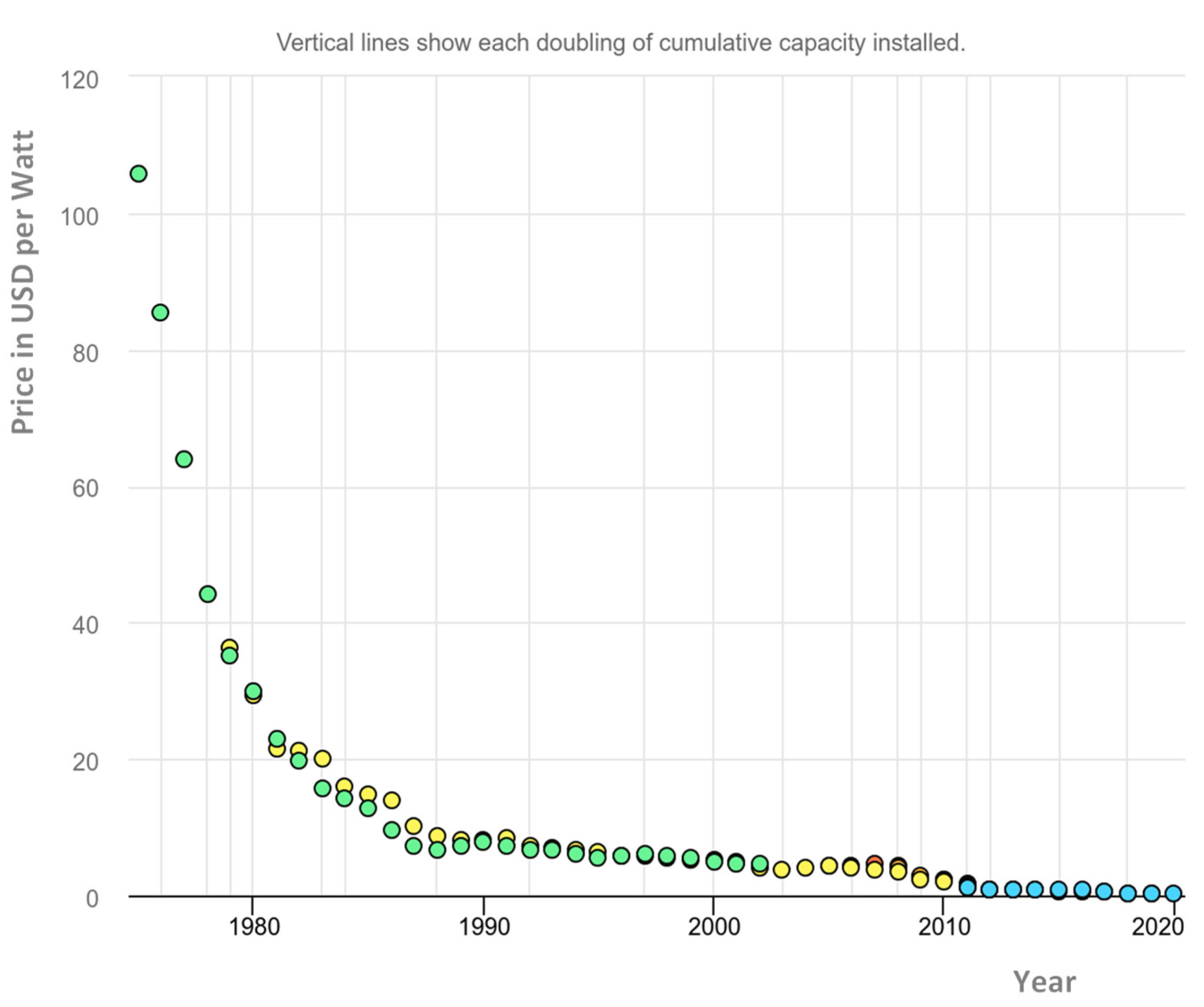
Figure 2.
Distribution of PV and wind turbine simulation papers by publisher.
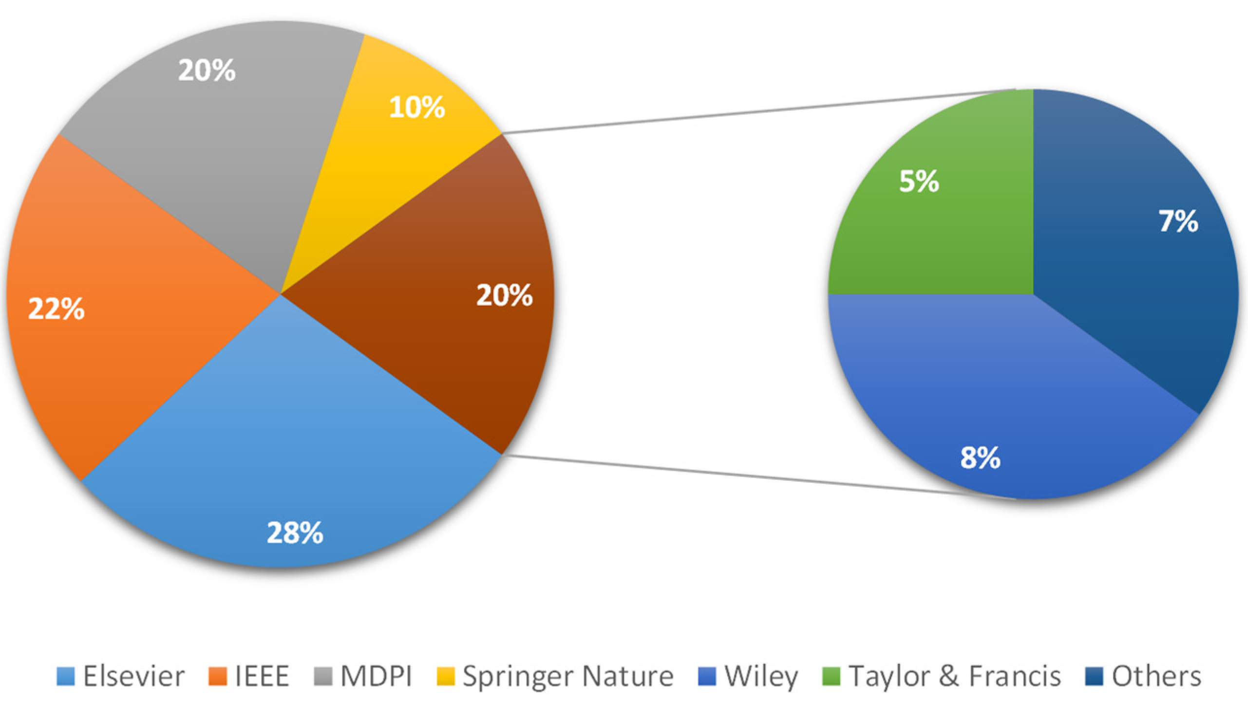
Figure 3.
Hierarchical classification of PV models.
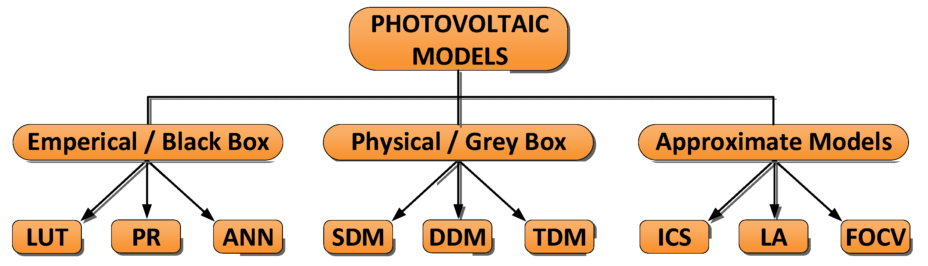
Figure 4.
SDM equivalent circuits for photovoltaic cells.
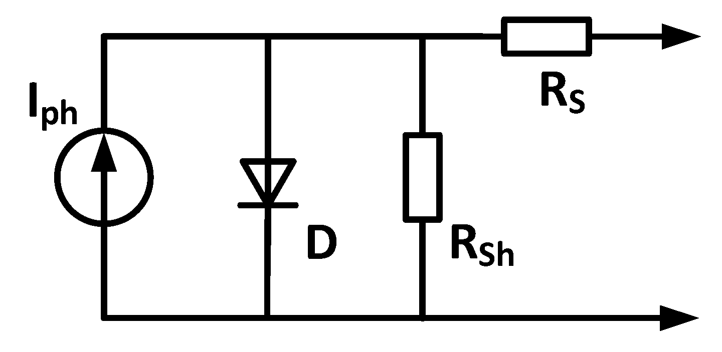
Figure 5.
SDM-based equivalent circuit for a photovoltaic powered pumping system.
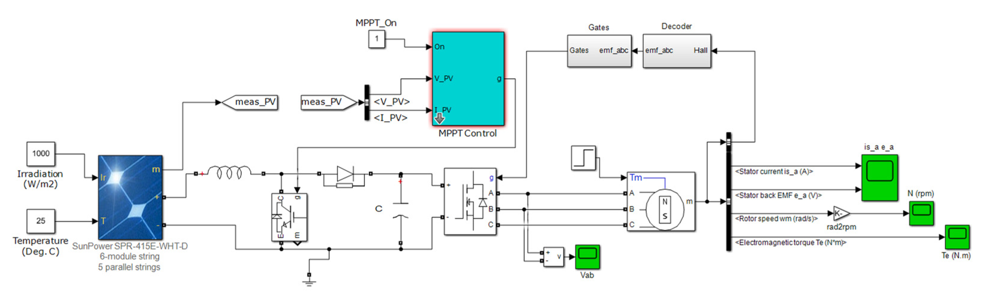
Figure 6.
DDM equivalent circuits for photovoltaic cells.
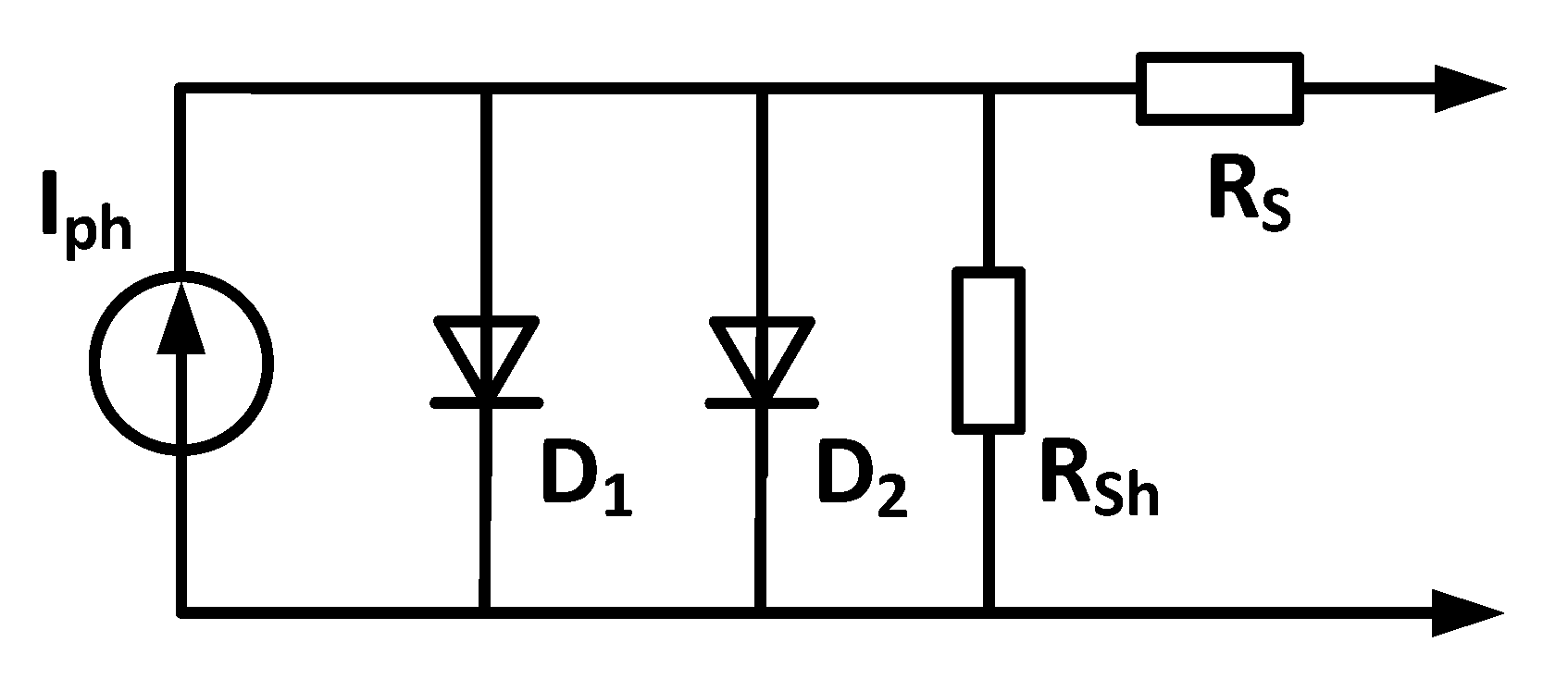
Figure 7.
Hierarchical classification of Wind Turbine models.
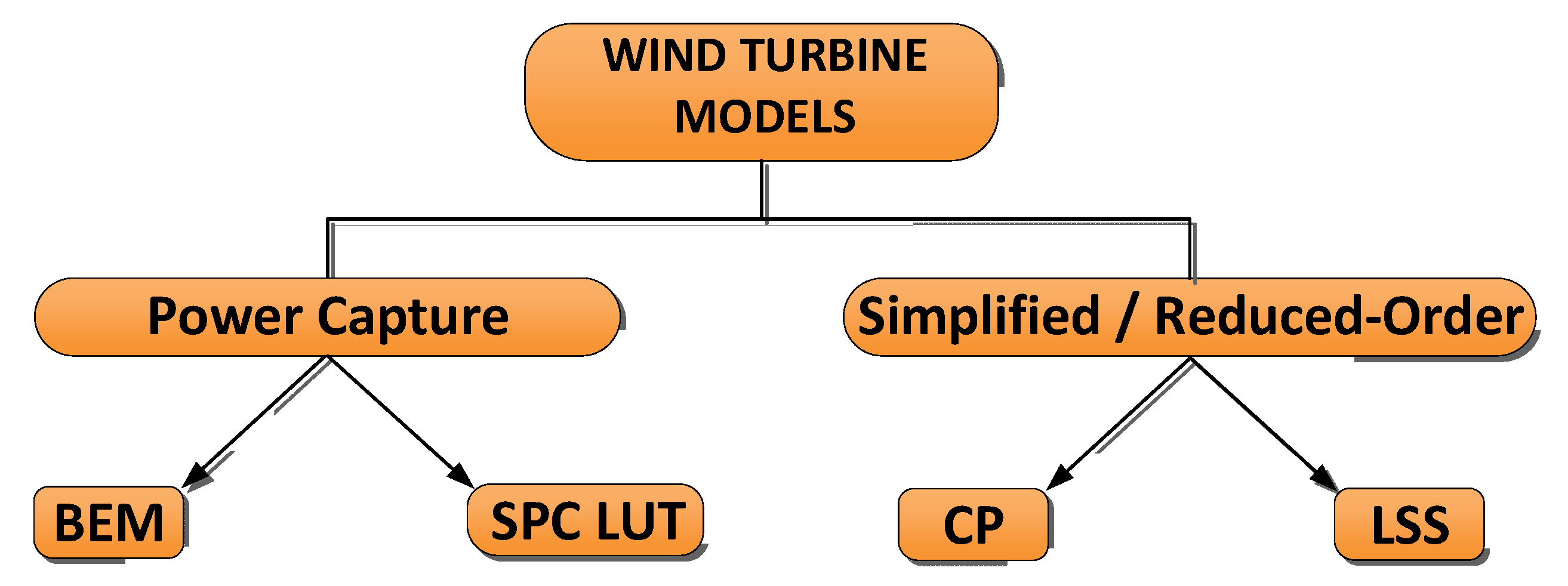
Figure 8.
Classification of main EMS categories for hybrid PV–WT.

Figure 9.
Simple rule-based EMS.
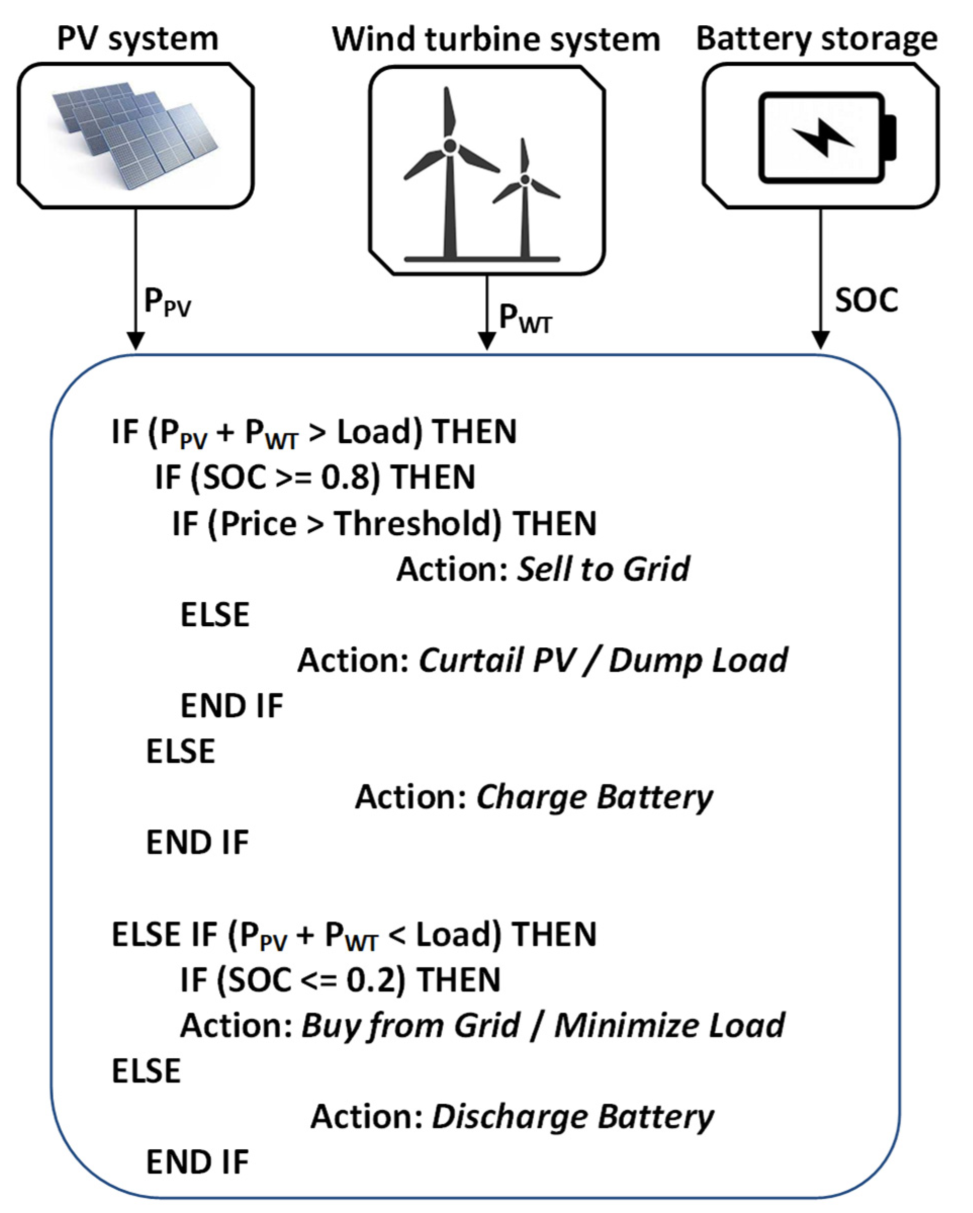
Figure 10.
RL EMS algorithm layout.
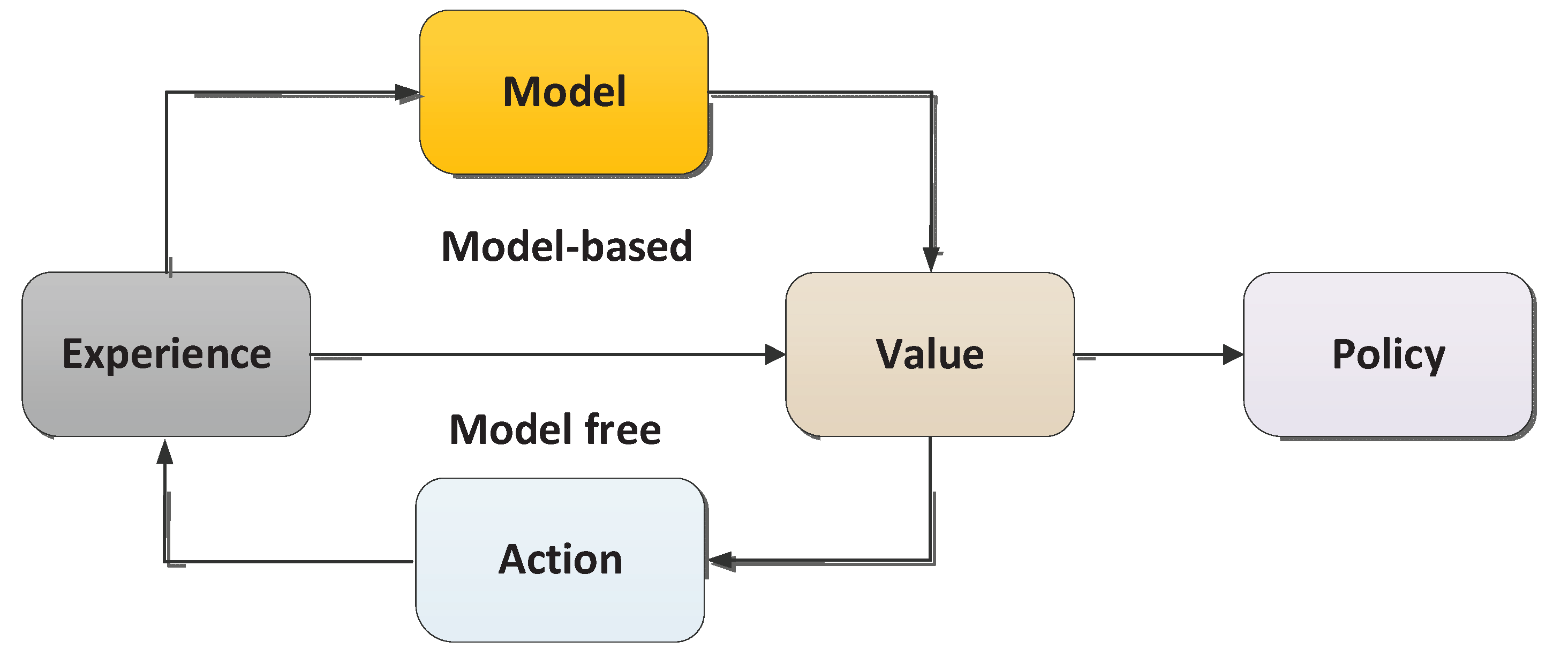

Table 1.
PV Simulation Tools Comparison.
| Simulation tool | Modeling Approach | Key Strengths |
|---|---|---|
| MATLAB/Simulink | Equation-based (custom models). | Flexibility, custom MPPT, co-simulation with other tools. |
| PV*SOL | 3D ray-tracing. | High accuracy, advanced 3D shading. |
| Helioscope | Cloud-native 3D modeling. | Web-based, rapid layout. |
| Solarius PV | 3D modeling + economic analysis. | High accuracy, integrated reporting. |
| HOMER Pro | Iterative optimization. | Multi-source optimization, energy management focus. |
| SolarGis | Satellite-derived irradiance. | High-resolution resource data, high accuracy simulation |
Table 2.
Wind Turbine Simulation Tools Comparison.
| Simulation tool | Primary Application | Key Strengths |
|---|---|---|
| MATLAB/Simulink | Control design, grid integration. | Flexibility, MPPT, education. |
| OpenFAST | Aero-hydro-servo-elastic simulation. | Industry standard, multi-physics. |
| AMR-Wind | High-fidelity CFD, wake modeling. | Blade-resolved, HPC scalability. |
| ROSCO | Controller design and tuning. | Open reference, OpenFAST compatible. |
Table 3.
Wind Turbine Simulation Tools Comparison.
| Feature | Rule-Based | Optimization-Based | Learning-Based |
|---|---|---|---|
| Decision Logic [107] | If-then-else rules | Mathematical programming | Neural network |
| Optimality | Suboptimal | Near optimal | Training-dependent |
| Computational Cost [108] | Very low | Medium to high | High |
| Training Required [109] | No | No | Yes |
| Handling Uncertainty [110,111] | Poor | Good | Good |
| Real-Time Feasibility [112] | Excellent | Good (if solver fast) | Excellent |
| Implementation Complexity [113] | Low | Medium to high | High |
| Typical Application [114] | Small off-grid systems | Grid-connected microgrids | Complex grid-connected microgrids |
Disclaimer/Publisher’s Note: The statements, opinions and data contained in all publications are solely those of the individual author(s) and contributor(s) and not of MDPI and/or the editor(s). MDPI and/or the editor(s) disclaim responsibility for any injury to people or property resulting from any ideas, methods, instructions or products referred to in the content. |
© 2026 by the authors. Licensee MDPI, Basel, Switzerland. This article is an open access article distributed under the terms and conditions of the Creative Commons Attribution (CC BY) license (http://creativecommons.org/licenses/by/4.0/).
Copyright: This open access article is published under a Creative Commons CC BY 4.0 license, which permit the free download, distribution, and reuse, provided that the author and preprint are cited in any reuse.


