

Submitted:
25 May 2026
Posted:
26 May 2026
You are already at the latest version
Abstract
Why does a quantum measurement yield one definite outcome rather than another? Decoherence theory explains the disappearance of interference, yet it leaves the selection of a particular result unexplained—and says nothing about what role, if any, the observer plays. This paper confronts both gaps head-on. We construct an Extended Hilbert Space HTotal=HPhys⊗HHigher in which information-processing agents carry their own quantum degrees of freedom, coupled to the physical sector through an explicit interaction Hamiltonian. The resulting Intention Field Theory (IFT) draws on von Neumann’s two-process picture and Stapp’s arguments for mental causation, but goes further by deriving—rather than postulating—a Lindblad-form master equation from the coupling term. Four results follow: agent-dependent decoherence rates that scale with intentional coherence; observer-dependent corrections to Born-rule probabilities; preferred-basis selection fixed by the measurement interaction; and an entropic quantification theorem linking intentional coupling to entropy production, physical–higher mutual information, and a Landauer heat-dissipation bound per measurement event. We test these predictions against eleven landmark experiments—quantum Zeno, which-path, delayed-choice, Bell-inequality, and matter-wave platforms among them—and find per-event entropy increases spanning 10−14 to 10−1 bits, depending on coupling strength and interaction time. When the intentional coupling is switched off, every prediction collapses back to standard quantum mechanics, so the framework is conservative by construction. We compare IFT with nine major interpretations and several dynamical-collapse models, map out the theory’s current limitations, and design specific falsification protocols. The mathematical development is deductive: axioms first, then lemmas, propositions with full proofs, and finally testable corollaries whose numerical signatures differ from those of all existing frameworks.
Keywords:
quantum measurement problem
; entropy production
; observer agency
; extended Hilbert space
; Lindblad master equation
; intentional coupling
; decoherence
; mutual information
; Landauer bound
; information-processing agents
1. Introduction
Quantum mechanics predicts the statistics of measurement outcomes with extraordinary precision, yet it is silent on a deceptively simple question: why does this outcome occur rather than that one? Despite nearly one hundred years of endeavor since Schrödinger, Heisenberg, and Bohr articulated the question [1,2], no resolution of the measurement problem has attained consensus [3,4].
Von Neumann [5] was the first to formalise the tension explicitly. His formulation distinguishes unitary evolution (Process 2, governed by the Schrödinger equation) from state reduction (Process 1, triggered upon measurement), and he noted that Process 1 involves a “free choice” by the observer—one not dictated by physical law. Stapp took this observation seriously [6,7]. He argued that quantum theory, as it stands, is incomplete: without accounting for the observer’s mental causation, no dynamical rule specifies when or why a superposition collapses. He further proposed the quantum Zeno effect as a concrete mechanism for mind–matter interaction.
Decoherence theory has made significant progress since then [8,9,10]. It explains convincingly why interference terms vanish in the reduced density matrix. What it does not explain is the emergence of a single definite outcome from the resulting mixture [11]—the so-called “and/or” problem. Wheeler and Zurek [12] collected perspectives spanning decades; the core puzzle has outlasted every attempt at resolution.
Spontaneous collapse models—GRW [13] and CSL [14]—take a different tack: they modify the Schrödinger equation itself so that superpositions of macroscopic distinctness decay automatically. The price is a set of new constants (collapse rate, localisation width) that must be tuned against experiment without deeper justification. Bassi and Ghirardi [15] surveyed these models and their empirical constraints in detail. Penrose [16] proposed that gravity triggers collapse; this is an interesting idea, but it too leaves the observer out of the picture.
Everett’s Many-Worlds interpretation [17,18] dispenses with collapse altogether—at the cost of a preferred-basis problem and unresolved difficulties with probability [19,20]. The pilot-wave formulation of Bohm and Hiley [21] restores determinism, yet it demands explicit nonlocality while yielding no new empirical content. Mermin [22] put the point memorably: the sheer persistence of interpretational disagreement hints that something about the role of information and observers has been missed. Bohr’s complementarity principle [23] and Schrödinger’s cat paradox [24] remain the touchstones of the debate.
Given the length and inconclusiveness of this debate, we contend that progress now requires formal mathematical structure rather than additional philosophical argumentation. In this paper we start from explicit postulates, introduce an intentional coupling Hamiltonian, and derive the consequences—including a Lindblad master equation, modified Born-rule probabilities, and entropic bounds—through standard proof techniques. The paper is organised as follows. Section 2 reviews consciousness-related quantum phenomena and the prior theoretical frameworks that motivate this work. Section 3 lays out definitions, axioms, and supporting lemmas. Section 4 proves the master equation and its physical predictions. Section 5 proposes experimental tests and compares IFT with existing interpretations. Section 6 applies the framework to eleven landmark experiments and offers concluding reflections.
2. Consciousness and Quantum Phenomena: A Critical Review
The question of whether the observer belongs inside the formalism of quantum mechanics or outside it has been debated since the 1920s, and remains far from settled. Before developing the mathematical framework that forms the core of this paper, we review the principal theoretical and experimental developments: what has been tried, what the experiments show, and where the existing proposals fall short.
2.1. Historical Development of Observer-Consciousness in Quantum Theory
The concept that observation assumes a foundational function in quantum mechanics can be traced to the initial formulations of the theory. Bohr’s complementarity principle [23] established that the experimental arrangement—chosen by the observer—determines which properties of a quantum system become manifest. Von Neumann [5] formalized this insight by distinguishing two processes: deterministic unitary evolution (Process 2) and non-deterministic state reduction upon measurement (Process 1). Crucially, von Neumann showed that the boundary between measured system and measuring apparatus—the so-called Heisenberg cut—can be shifted arbitrarily along the measurement chain without altering predictions, terminating only at the observer’s consciousness. This logical structure, sometimes called the von Neumann chain, placed the observer’s subjective experience at a foundational position in the theory’s formalism.
London and Bauer [25] made this implication explicit in 1939, arguing that the observer’s faculty of introspection—the ability to create a new objectivity by asserting “I am in state x”—is what distinguishes measurement from ordinary physical interaction and thereby resolves the measurement problem. Wigner [26] further developed this position, contending that consciousness is necessary for the collapse of the wavefunction and that the linearity of quantum mechanics must break down when conscious beings are involved. Wigner’s friend paradox, which accentuates the discord between two observers’ descriptions of the identical quantum occurence, persists as a pivotal thought experiment in quantum foundations [27,28].
Stapp [6,7,29] provided perhaps the most sustained modern defense of observer participation in quantum mechanics, building on von Neumann’s Process 1 to argue that the observer’s “free choice” of which question to pose to nature—the probing action—is a genuinely causal act not reducible to physical law. Stapp identified the quantum Zeno effect as a specific mechanism through which mental effort could stabilize neural quantum states, thereby influencing brain dynamics and, through them, physical reality. His account preserves the causal closure of physics at the level of the total (psychophysical) system while allowing irreducible mental causation at the level of Process 1.
Pauli’s collaboration with Jung on synchronicity [30] and Wheeler’s “participatory universe” [31] represent further historical threads connecting observation, information, and physical reality. Wheeler’s delayed choice gedanken experiment demonstrated that the observer’s present choice of measurement can determine the description of past events, reinforcing the view that observation is not passive recording but active participation in the constitution of physical phenomena.
2.2. Contemporary Theoretical Frameworks
Among contemporary theoretical efforts, four initiatives are characterized by their breadth and accuracy. Each addresses a distinct facet of the consciousness–quantum interface, bringing notable strengths alongside identifiable limitations.
2.2.1. Orchestrated Objective Reduction (Orch-OR)
Penrose [16,32] proposed that quantum state reduction is an objective physical process triggered when gravitational self-energy of the superposition reaches a threshold , where is the collapse timescale. Hameroff and Penrose [33] combined this gravitational collapse mechanism with a biological substrate: microtubules within neurons, whose tubulin protein conformations are hypothesized to sustain quantum coherence long enough for orchestrated objective reduction to occur. The theory predicts that consciousness arises when orchestrated quantum computations in microtubule networks undergo objective reduction at the Diósi-Penrose threshold [34].
Orch-OR has been criticized on multiple grounds. Tegmark [35] calculated that decoherence timescales in warm, wet biological environments ( s for microtubule superpositions) are approximately 10 orders of magnitude shorter than the timescales relevant to neural processing (– s), arguing that quantum coherence cannot be maintained in brain tissue. Hameroff and Penrose [33] responded by citing evidence for quantum effects in biological systems, including quantum coherence in photosynthesis [36] and avian magnetoreception [37], though the relevance of these specific mechanisms to neural microtubules remains debated. The Diósi-Penrose collapse threshold has been experimentally constrained by optomechanical experiments [38,39], with results narrowing but not yet excluding the parameter space.
Orch-OR is arguably the most falsifiable consciousness–quantum proposal available: it names a substrate (microtubules), writes down a collapse condition (), and predicts a timescale. That specificity is rare in this field. The obstacle is that all of these merits depend on one untested assumption—that quantum coherence in microtubules persists within the thermal, aqueous environment of a living neuron. Three decades of experimental effort have not demonstrated this in vivo. There is also a logical gap worth flagging: the gravitational collapse threshold is a physics claim, testable in principle through optomechanical experiments, whereas the assertion that such collapse in microtubules produces consciousness is a neuroscience claim with no independent evidence. Confirming the former would not establish the latter.
2.2.2. Quantum Brain Dynamics
Umezawa and collaborators [40,41] proposed Quantum Brain Dynamics (QBD), applying quantum field theory to the brain’s water molecules and electromagnetic field. In this framework, the electric dipole field of water molecules confined within neuronal membranes supports coherent quantum states through dynamical symmetry breaking, producing Nambu-Goldstone bosons (termed “corticons”) that serve as quantum carriers of mental information. Vitiello [42,43] extended this into a dissipative quantum field theory model, arguing that memory arises from the multiplicity of unitarily inequivalent representations in infinite-dimensional quantum field theory, naturally explaining memory capacity and recall without the decoherence difficulties facing finite-dimensional proposals.
QBD avoids some of Tegmark’s decoherence objections by operating at the level of collective field excitations rather than individual molecular superpositions. However, it remains unclear whether the coherent dipole oscillations postulated by QBD can be experimentally distinguished from classical electromagnetic field dynamics in neural tissue.
QBD is, in many respects, the mirror image of Orch-OR. Its use of quantum field theory rather than finite-dimensional quantum mechanics sidesteps Tegmark’s decoherence bound entirely, and Vitiello’s dissipative extension—which exploits the system–environment doubling to explain memory without information loss—is mathematically elegant. The cost of this elegance is empirical thinness. QBD does not tell us what measurement, performed on what system, would come out differently if QBD-mediated cognition is real versus if ordinary classical neural computation suffices. No effect size is predicted for any conceivable experiment. Where Orch-OR commits to specific empirical predictions, QBD remains uncommitted—and consequently faces the risk of unfalsifiability.
2.2.3. The Beck-Eccles Model
Beck and Eccles [44] proposed that quantum tunneling processes at synaptic vesicle release sites provide a mechanism for mental causation in the brain. Their model identifies the exocytosis probability at synaptic boutons as the locus of quantum indeterminacy, with the conscious mind influencing which synaptic vesicles are released through modification of tunneling probabilities. At characteristic energies of eV and length scales of nm, these processes lie firmly within the quantum-mechanical domain. However, the model does not specify the mechanism by which consciousness influences tunneling rates, leaving the central explanatory gap unfilled.
Of the four proposals reviewed here, the Beck-Eccles model is arguably the least vulnerable to the decoherence critique: synaptic tunnelling operates at energy scales ( eV) and length scales ( nm) where nobody disputes the relevance of quantum mechanics. The problem, however, is of a different sort. Beck and Eccles identify where consciousness might couple to quantum dynamics—at the synaptic bouton—yet remain silent on how. The mind is said to modify tunnelling probabilities, yet no dynamical equation governs this modification. It is precisely this kind of gap—a missing coupling Hamiltonian—that motivated the construction of in the present work. A second, less discussed worry: even granting that consciousness influences exocytosis at individual synapses, neural networks are highly redundant and noise-tolerant. Whether single-synapse quantum effects can propagate to macroscopic cognition is far from obvious.
2.2.4. Integrated Information Theory
Tononi’s Integrated Information Theory (IIT) [45,46,47] identifies consciousness with integrated information (), a mathematical quantity measuring the degree to which a system generates information above and beyond its parts. While IIT is primarily a classical information-theoretic framework, its axioms and postulates have been explored in quantum settings [48], where entanglement can contribute to integration. IIT’s panpsychist implications—that any system with possesses some degree of consciousness—resonate with aspects of quantum observer theories, though IIT itself does not require quantum mechanics for its core formalism. The theory’s principal limitation is computational: calculating is intractable for systems larger than approximately 20 elements, making empirical validation of its central claims exceedingly difficult.
IIT holds a unique status in this examination: it does not necessitate quantum mechanics at all. Its axioms (existence, composition, information, integration, exclusion) yield a scalar measure of consciousness, , that can in principle be computed for any system—quantum or classical. That makes it immune to the decoherence objection, which is a real advantage. But it also means IIT has nothing to say about the measurement problem, Born-rule probabilities, or any quantum-mechanical observable. For the purposes of the present paper, IIT is orthogonal rather than competitive. Two additional concerns deserve mention: the theory’s panpsychist commitment (any system with is, to some degree, conscious—including a photodiode) strikes many physicists as counterintuitive; and computing for systems larger than ∼20 elements is computationally intractable, making the theory’s central prediction effectively untestable for biological brains.
2.2.5. Comparative Effectiveness of Contemporary Frameworks
Taken together, these four programmes each make a genuine contribution, yet each is incomplete in a different way. Orch-OR commits to a specific substrate and collapse mechanism, yielding falsifiable predictions that are, however, under pressure from decoherence data. QBD is mathematically sophisticated but does not generate testable predictions. Beck-Eccles pinpoints a plausible interaction site without supplying dynamics. IIT sidesteps quantum mechanics entirely.
What none of them provides is a derived master equation—an equation of motion for the physical density matrix, obtained from an explicit coupling Hamiltonian linking observer degrees of freedom to quantum observables. Orch-OR postulates a collapse trigger but never derives the resulting dynamics from a coupling term. QBD describes the field-theoretic structure but predicts no measurable deviation from standard quantum mechanics. Beck-Eccles locates the quantum process at the synapse but leaves the coupling unspecified. IIT quantifies consciousness through but makes no contact with quantum dynamics whatsoever. This shared absence—a Hamiltonian-derived, Lindblad-form master equation—is the gap we set out to fill in Section 3 and 4.
2.3. Experimental Investigations of Consciousness-Quantum Interactions
Can consciousness actually do anything to a quantum system, or is the whole idea empirically empty? Several experimental initiatives have attempted to resolve the issue. The results are controversial, but they cannot simply be ignored: any theoretical proposal that claims observer agency matters must eventually be measured against them.
2.3.1. Random Event Generator Studies
The Princeton Engineering Anomalies Research (PEAR) laboratory conducted extensive investigations over nearly three decades (1979–2007) into whether human intention could influence the output of random event generators (REGs) [49,50]. The PEAR REG devices employed electronic noise diodes (typically Zener diode reverse-bias junctions at –8 V) operating at room temperature ( K), generating random bits at rates of 200–1000 bits/s with hardware autocorrelation . Operators were seated at distances of –2 m from the device, with trial durations of –50 s per run. Across approximately trials involving 91 operators, the program reported small but statistically significant deviations from chance expectation correlated with operator intention, with a mean effect size of approximately bits per trial. A comprehensive meta-analysis by Bösch et al. [51] covering 380 studies confirmed a small overall effect (, ) but noted that effect sizes were heterogeneous across laboratories and correlated with methodological quality, raising concerns about publication bias and selective reporting. Alcock [52] provided systematic critiques of the parapsychological evidence, questioning whether the observed effects survive rigorous methodological scrutiny.
The Global Consciousness Project [53] extended REG methodology to a network of devices distributed worldwide, testing whether collective human attention during major global events correlates with deviations from randomness. Results have been reported as statistically significant, though the post-hoc selection of events and analysis windows remains a point of contention.
The REG data present an uncomfortable pattern. Cumulative statistics across thousands of sessions yield p-values that look impressive, yet individual effect sizes are tiny—around bits per trial—and, crucially, they shrink as experimental rigour increases. The Bösch et al. meta-analysis [51] found an inverse correlation between effect size and study quality. That is the signature one expects from publication bias or uncontrolled artifacts, not from a genuine physical coupling. A deeper problem is the absence of a predictive model: without specifying how consciousness biases a Zener-diode noise source, a bare statistical anomaly cannot be distinguished from a systematic error.
For our purposes, the REG literature is useful not as evidence that the effect is real, but as an upper bound. If intentional coupling exists at all, its strength must be consistent with the very small reported deviations. The implied magnitude, (Lemma 2), serves as an empirical anchor throughout the rest of the paper.
2.3.2. Double-Slit Consciousness Experiments
Radin et al. [54,55] conducted systematic experiments testing whether focused human attention could modulate a double-slit interference pattern. The apparatus consisted of a 5 mW HeNe laser ( nm) illuminating a double-slit assembly (slit width m, slit separation m) with the interference pattern recorded by a 16-bit CCD camera (active area , pixel pitch m) at a distance of m from the slits. The optical path was enclosed in a triple-shielded chamber (Faraday cage with dB electromagnetic attenuation at 1 GHz), maintained at room temperature ( K) with thermal stability K over experimental sessions. Participants were positioned at distances of –3 m from the apparatus, with alternating attention-toward and attention-away epochs of 15–30 s duration. The researchers measured the spectral ratio of double-slit to single-slit spectral power during these epochs. Across six experiments with 137 participants (50 experienced meditators, 87 non-meditators), the combined result yielded (), with meditators producing significantly stronger effects than non-meditators ( versus ). Control sessions (1153 total) without observers showed no effect ().
These results, while striking, await independent replication by groups outside the original research team. The small effect sizes and potential for subtle environmental confounds (despite extensive shielding) demand caution in interpretation. Several attempted replications have yielded mixed results, underscoring the need for preregistered, multi-laboratory protocols with rigorous blinding.
2.3.3. Neuroscience of Quantum-Consciousness Claims
Neuroimaging and electrophysiological studies have sought neural correlates that might mediate consciousness-quantum interactions. Fisher [56] proposed that nuclear spins of phosphorus atoms (31P, spin-, natural abundance 100%) in Posner molecules (, diameter nm) could serve as biological qubits with coherence times estimated at – s (hours to days) at body temperature ( K), protected from decoherence by the tetrahedral symmetry of the groups which suppresses electric quadrupole interactions. The estimated spin-spin coupling within a Posner cluster is –10 Hz, potentially sufficient for entanglement generation on biologically relevant timescales. This “quantum cognition” proposal is notable for identifying a specific biochemical mechanism that could sustain quantum coherence at biological temperatures, though experimental confirmation of Posner molecule quantum coherence in vivo remains lacking.
Koch and Hepp [57] argued that the vast majority of proposals connecting quantum mechanics to consciousness fail because they either invoke quantum effects where classical descriptions suffice or require coherence timescales incompatible with neural dynamics. The fundamental premise of their argument is that proponents of quantum consciousness possess the responsibility to demonstrate that quantum coherence performs a computational role in neural networks which classical dynamics alone cannot reproduce.
2.4. Assessment and Motivation for the Present Work
What lessons should we draw from all of this? We see five that bear directly on the construction attempted in the next sections.
The measurement problem is still open. Decoherence has not solved it [3,10]. Interference terms disappear from the reduced density matrix, yes—but the question of why one outcome obtains rather than another is exactly where decoherence falls silent [11]. The “and/or” problem persists.
Observer-collapse ideas lack equations. From von Neumann’s original observation to Stapp’s sustained philosophical arguments, the case for observer agency in quantum mechanics has been stated in words. What has been missing is a coupling Hamiltonian, a derived master equation, and numerical predictions that could be checked against data. Supplying these is the aim of the present paper.
If the effect is real, it is very weak. The Radin experiments [54] report decoherence-rate shifts of order –. Whether or not those particular results survive further replication, they set the scale: any intentional coupling must be feeble enough to have escaped routine detection. Our estimate, , is consistent with this constraint and with the obvious fact that people do not collapse wavefunctions by thinking hard in everyday life.
Existing theories each leave something out. Orch-OR is bold but fragile; QBD is safe but vague; Beck-Eccles identifies a site without a mechanism; IIT is self-contained but ignores quantum mechanics. None derives a master equation from a coupling Hamiltonian. Our approach fills this gap by remaining agnostic about the physical substrate of intentional states and working instead at the level of abstract Hilbert-space degrees of freedom, coupled to quantum observables through an explicit .
We need explicit criteria for success. Any theory of this kind should satisfy at least the following: (i) mathematical consistency—well-defined Hilbert-space structure with positive, trace-preserving dynamics; (ii) decoherence resilience—the proposal must not be killed by thermal noise in biological systems; (iii) falsifiability—specific, quantitative deviations from standard quantum mechanics must be predicted; (iv) explanatory completeness—a dynamical mechanism, not merely an interaction site; and (v) substrate independence—no reliance on unverified claims about particular biological structures. Whether the framework developed below actually meets all five is for the reader to judge; that it is designed to meet them should become clear as the axioms and proofs are laid out.
3. Definitions and Axioms
3.1. Definitions
Definition 1
(Physical Hilbert Space). The Physical Hilbert Space is the complex separable Hilbert space in which standard quantum mechanical states reside, equipped with inner product and satisfying the axioms of quantum mechanics as established by von Neumann [5].
Definition 2
(Extended Hilbert Space). The Extended Hilbert Space for an information-processing system S is the tensor product
where contains degrees of freedom orthogonal to spacetime, such that . The architecture of and its subspaces is illustrated in Figure 1.
Remark 1.
Definition 3
(Intention). An intention is an internal representational state of an information-processing system that encodes a disposition toward particular measurement outcomes or physical configurations. Intentions are not necessarily conscious or deliberate; they represent the system’s internal orientation toward specific states in . Intentions are not directly observable in but manifest through coupling to physical degrees of freedom.
Definition 4
(Expression). An expression is an externally manifested configuration through which an information-processing system’s internal states couple to the physical world. Expressions represent the actualized interface with , whether through measurement apparatus settings, motor outputs, or any physical configuration mediating the interaction with observed quantum systems.
Definition 5
(Intentional Space). The Intentional Space is the subspace where are orthonormal basis states representing distinct intentions, and with M the intentional dimensionality determined by the information-processing capacity of system S.
Definition 6
(Expressive Space). The Expressive Space is the subspace where are orthonormal basis states representing distinct expressions, and with K the expressive dimensionality of system S.
Definition 7
(Intention Operator). The Intention Operator is the Hermitian operator
where denote the eigenvalues representing the intentional potential of each mode.
Remark 2.
Definition 8
(Expression Operator). The Expression Operator is the Hermitian operator
where are eigenvalues representing the expressive clarity of each mode.
Definition 9
(Alignment Operator). The Alignment Operator quantifying the internal coherence is
where are fundamental constants defining correspondence between intention m and expression k.
Definition 10
(Universal Coupling Constant). The Universal Coupling Constant g has dimensions and quantifies the fundamental strength of coupling between the intentional and physical degrees of freedom.
Definition 11
(Mode-Coupling Strength). The Mode-Coupling Strength for intentional state has dimensions [Intentional Potential] and determines the efficacy with which that intentional mode couples to physical observables.
Definition 12
(Characteristic Length Scale). The Characteristic Length Scale is the fundamental length scale at which intentional coupling is defined, corresponding to the atomic-scale quantum coherence typical of molecular and condensed matter systems.
Definition 13
(Intentional Potential Unit). One Intentional Potential (1 IP) is defined operationally by fixing a standard reference system and a reference decoherence effect. The standard reference system consists of a single electron in a harmonic potential with frequency , prepared in the spatial superposition with . A mode-coupling strength of , combined with a single focused intentional mode (), produces in this reference system an additional decoherence rate beyond the environmental baseline. This definition, together with Proposition 6, uniquely determines the numerical value of the coupling constant g.
3.2. Axioms and Laws
Axiom 1
(Extension of State-Space). Every information-processing system capable of representing and interacting with quantum states possesses degrees of freedom in the Extended Hilbert Space .
Remark 3
(Structural versus Agent-Mediated Coupling). Axiom 1 defines “information-processing system” broadly: any physical system configured to represent and interact with quantum states—including measurement apparatus, detectors, and feedback-controlled experimental protocols—possesses degrees of freedom in . This yields a natural two-layer decomposition of the intentional decoherence rate:
Structural coupling is activated whenever a measurement configuration extracts which-state information from a quantum system; it depends on apparatus parameters (detector efficiency, measurement basis, spatial separation) but is independent of whether a conscious agent is present.Agent-mediated coupling is an additional contribution arising when a conscious intentional agent directs focused attention toward the system. The structural layer ensures that IFT’s predictions for measurement-induced decoherence are consistent with automated, unobserved experiments—resolving the question of “whose intention?” by grounding the baseline coupling in the information-extracting structure of the protocol itself. The agent layer provides a testable enhancement: experiments comparing outcomes with and without trained intentional agents (Section 5.1–5.11) directly probe , with the Radin double-slit experiments (Section 5.8) constituting the most direct existing test.
Axiom 2
(Orthogonality of Higher Space). The higher-dimensional space is orthogonal to spacetime coordinates, representing an abstract state space analogous to spin space rather than geometric extra dimensions.
Remark 4.
Law 1
(Law of Intentional-Physical Interaction). An agent with an intentional state in couples to a physical system through the interaction Hamiltonian
where is the position operator of system and is the characteristic length scale.
Remark 5.
The Law of Intentional-Physical Interaction establishes position as the coupling observable because position is the most fundamental classical observable [64], measurements typically localize systems in position space [65], linear coupling represents minimal interaction analogous to dipole coupling in quantum electrodynamics [66], and alternative couplings to momentum or spin could be explored in future investigations. The choice of position coupling is not unique but represents the simplest and most natural starting point. The characteristic length scale ensures dimensional consistency and reflects the atomic-scale regime, where quantum coherence is typically maintained [3]. In subsequent derivations, we employ the reduced coupling constant , which has dimensions , so that . The effective coupling absorbs the bath correlation timescale (see Proposition 6 proof). For notational brevity, we write g in place of throughout the remainder of this paper; all instances of g in Section 4–6 refer to this reduced effective coupling, and the numerical estimate (Lemma 2) incorporates .
Law 2
(Law of Weak Coupling). The interaction Hamiltonian satisfies where is the free Hamiltonian, ensuring perturbative treatment remains valid.
Remark 6.
Weak coupling is a familiar working assumption in quantum optics [67] and cavity QED [68]. Perturbative series converge provided the interaction strength remains well below the dominant energy scales of the free Hamiltonian—a requirement comfortably satisfied by the numerical bound established in Lemma 2.
Law 3
(Conservation of Probability). All dynamical evolution in preserves trace and positivity: for all t and for all t.
3.3. Lemmas
Lemma 1
(Dimensional Consistency). The coupling constant g, mode strengths , and characteristic length must satisfy the following:
to ensure has the correct dimensions. Here denotes the dimensions of the position operator’s eigenvalues (Length).
Proof.
From the definition of in the Law of Intentional-Physical Interaction, each term has the form . Since is a Hamiltonian, it must have dimensions of Energy. The position operator’s eigenvalues have dimensions of Length, and has dimensions of Length. Therefore , whence . The reduced coupling then has dimensions , and , confirming that has the required energy dimensions. This dimensional analysis follows standard practice in theoretical physics [72]. □
Corollary 1.
The universal coupling constant has dimensions
and mode coupling strengths have dimensions
Lemma 2
(Order-of-Magnitude Estimation). For focused intention with , characteristic coupling strength , and position separation , requiring intentional decoherence to produce the standard reference rate (Definition 11) yields a reduced coupling constant
corresponding to an unreduced coupling .
Proof.
From Proposition 6 (proven below), the intentional decoherence rate for a superposition with spatial separation is (where g is the reduced coupling ). For focused intention, , and at the characteristic separation . Setting gives , hence . Substituting , , , and yields . The unreduced coupling is , which characterizes the coupling strength at the reference scale . The dimension arises because the Proposition 6 formula absorbs the bath correlation time into the effective coupling (see proof of Proposition 6). For notational convenience, in subsequent sections we write g and quote with the understanding that has been absorbed into the reduced coupling (see Remark following Law 1). The numerical estimate employs standard order-of-magnitude techniques [73]. □
Remark 8.
The numerical value is aneffectivereduced coupling that absorbs the bath correlation time (see Proposition 6 proof). The bare coupling constant appearing in has dimensions (Lemma 1); the additional arises from integrating out the bath correlation function in the Born-Markov approximation. This extraordinarily weak coupling explains the absence of macroscopic intentional effects in everyday experience. Only in highly isolated quantum systems at low temperatures, where environmental decoherence is suppressed below [3,10], do intentional effects become comparable to environmental effects and thus potentially observable.
Lemma 3
(Born Approximation). Under the Law of Weak Coupling, the total density matrix remains approximately factorized:
to second order in .
Proof.
The exact evolution is where is the time evolution operator [63]. Expanding in powers of using and the Magnus expansion [74,75], and assuming uncorrelated initial conditions , the first-order correction vanishes if in the initial state. The second-order correction produces correlations of order , justifying the factorization to leading order. This Born approximation is standard in open quantum systems theory [76]. □
Lemma 4
(Markov Property). If the correlation time of intentional states satisfies where is the characteristic evolution time of , then the reduced dynamics of depend only on the current state and not on history.
Proof.
The memory kernel in the exact master equation [76] is which decays on the timescale . The correlation function satisfies for [77]. For , the integral by pulling out of the integral since varies slowly compared to K’s decay. This establishes the Markov property following the standard Nakajima-Zwanzig projection operator formalism [78,79]. □
Remark 9.
The validity of this lemma for cognitive systems warrants careful scrutiny. Intentional states in human agents persist over seconds to minutes (–), while the characteristic evolution time of quantum systems of interest ranges from nanoseconds for superconducting qubits () to microseconds for trapped ions (). Since in all cases of practical interest, the Markov condition is violated. However, the opposite limit corresponds to a quasi-static intentional state, which simplifies rather than complicates the dynamics: the intentional state can be treated as approximately constant during the physical system’s evolution, and the Born-Markov master equation remains valid with replaced by its time-averaged value. Generalisations to non-Markovian dynamics via memory-kernel formalisms [80,81] are taken up in Section 5.3.
4. Propositions and Theorems
4.1. Derivation of the Master Equation
Proposition 1
(Interaction Picture Evolution). In the interaction picture defined by , the evolution satisfies:
where .
Proof.
By definition, . Taking the time derivative:
Proposition 2
(Formal Integration). The interaction picture density matrix satisfies
Proof.
Direct integration of Proposition 1 from zero to t. This is a formal solution to the first-order differential equation [82]. □
Proposition 3
(Second-Order Evolution). To second order in , the evolution equation becomes
Proof.
Substituting the formal integration result from Proposition 2 into the original evolution equation (Eq. 11), replacing in the integrand. This yields a second-order expansion in powers of :
Proposition 4
(Reduced Dynamics Under Born Approximation). Tracing over the intentional degrees of freedom and applying the Born approximation yields
Proof.
The partial trace operation is applied to the second-order evolution equation (Eq. 14). This procedure embodies a completely affirmative, trace-preserving (CPTP) map [58,69]. The first-order term vanishes, assuming , which holds when the intentional state has a zero mean in the coupling basis. Apply the Born approximation (Lemma 3) where is the quasi-static intentional state. This approximation is valid under weak coupling and justified by the factorization property proven in Lemma 3. □
Proposition 5
(Markovian Master Equation). Under the Markov approximation, extending integration to infinity and replacing yields
Proof.
The integration variable is changed from s to . Under the Markov property (Lemma 4), the state can be replaced by since the density matrix varies slowly compared to the correlation time of the memory kernel. The upper limit can be extended to infinity because the memory kernel decays exponentially for [76,84]. This Markovian master equation derivation follows the standard projection operator technique [78,79,85]. □
Theorem 1
(IFT Master Equation). The reduced density matrix of the physical system under intentional influence evolves in the Schrödinger picture as follows:
where the intentional dissipator is
and is the probability of an intentional state .
Proof.
From the Law of Intentional-Physical Interaction (Eq. 5), where we used the static intentional state assumption that is time-independent in the interaction picture. Evaluating the double commutator in Eq. (17):
Using orthogonality and the trace property where is the probability of being in the intentional state , we obtain:
Corollary 2
(Lindblad Form). The dissipator has a Lindblad form, ensuring complete positivity and trace preservation.
Proof.
The double commutator structure is the standard Lindblad form [71] guaranteed by the Gorini-Kossakowski-Sudarshan theorem [70] to preserve complete positivity and trace. Specifically, for any operator , the superoperator
is the most general form of a Lindblad dissipator, preserving trace and complete positivity [86]. The double commutator in Eq. (19) can be rewritten in this standard form, establishing the result. □
Remark 10.
The Lindblad structure is essential for ensuring that the dynamics remain physical. Complete positivity prevents evolution into unphysical negative probability states, while trace preservation ensures normalization [69,87]. The complete mechanism by which intentional coupling produces decoherence and modified Born rule predictions is depicted schematically in Figure 2.
4.2. Physical Predictions
Proposition 6
(Intentional Decoherence Rate). The decoherence rate induced by intentional coupling for a spatial superposition with separation is
where g denotes the reduced coupling constant with dimensions as defined following Law 1.
Proof.
From Theorem 1, the intentional dissipator in the position representation yields the decoherence term (cf. Proposition 7, Eq. 26):
where is the position autocorrelation function, which is dimensionless when is measured in the units absorbed into the reduced coupling g. The integral evaluates to a timescale of order unity in the natural units of the system (set by where is the characteristic energy scale). For the standard reference system defined in Definition 11, , which is absorbed into the numerical value of g. The resulting off-diagonal decay is exponential:
with [3,10]. Dimensional verification: Since g is the effective coupling absorbing , . Then ; multiplying by and yields . This confirms . □
Corollary 3
(Recovery of Standard Quantum Mechanics). When , we have and the master equation reduces to standard quantum mechanics. When with , the dissipator does not vanish but produces a uniform decoherence rate independent of the agent’s state, indistinguishable from an environmental contribution.
Proof.
Setting eliminates the intentional interaction entirely (), whereupon Eq. (18) collapses to the ordinary Liouville-von Neumann evolution [5,63]. For , the sum reduces to a single term: with . This is nonzero if , but since there is only one intentional mode, the decoherence rate is a fixed constant independent of the agent’s intentional state distribution. Such a state-independent contribution is operationally indistinguishable from environmental decoherence and can be absorbed into the environmental decoherence rate . The agent-dependent predictions of IFT therefore require , corresponding to an agent capable of directing intention among distinct modes. □
Corollary 4
(Agent Control). For focused intention on state k with , the decoherence rate is controlled by the intentional state of the agent.
Proof.
When , the probability distribution is peaked: . Therefore , giving . □
Corollary 5
(Preferred Basis). The intentional dissipator induces position as the preferred basis through coupling to .
Proof.
Theorem 2
(Entropic Quantification of Intentional Coupling). Let denote the reduced density matrix of a physical system initially prepared in the spatial superposition with separation , evolving under the intentional decoherence of Proposition 6 at rate . Then:
- (i)
-
Entropy evolution.The von Neumann entropy of the physical subsystem iswhere is the binary entropy function, increasing monotonically from (pure state) at to (one bit) as .
- (ii)
-
Two-layer entropy decomposition.Under the decomposition (Eq. 5), the agent-mediated entropy enhancement at observation time τ iswhich is directly measurable by comparing entropy in with-agent versus without-agent conditions.
- (iii)
-
Mutual information.If the total state in remains pure during the coupling, the mutual information satisfiesEvery bit of coherence lost by the physical subsystem generates two bits of correlation with : information is not destroyed but transferred.
- (iv)
-
Landauer bound.The minimum energy dissipated during intentional decoherence satisfieswhere T is the environment temperature. Complete decoherence of one qubit requires at least of energy, providing a thermodynamic consistency requirement for the coupling constant g.
Proof
Part (i). From Proposition 6, the off-diagonal elements of in the position basis decay as . The density matrix of the two-state superposition takes the form
with eigenvalues . The von Neumann entropy [5,58]. At : , , giving . As : , giving . Monotonicity follows from and the strict concavity of on : both derivatives are negative, so their product [58].
Part (ii). Substituting into Part (i), the entropy with agent present is and without agent is . Since , the argument of in is no greater than in , and since is monotonically decreasing on , we have . For , Taylor expansion gives , confirming linear dependence on agent coupling strength.
Part (iii). The evolution under in is unitary (Law 3, Conservation of Probability), preserving at all times. For a bipartite pure state, the Schmidt decomposition gives [58]. The mutual information is therefore [58,87]. Physically, coherence information is not destroyed by intentional decoherence but transferred to correlations between and .
Part (iv). Landauer’s principle [88,89] states that erasing of information from a system in thermal contact at temperature T requires minimum energy dissipation . The intentional decoherence process erases coherence information from , increasing its entropy by . Complete decoherence () erases one bit (), requiring . At K, J, consistent with the weak-coupling regime (Law 2) since while the coupling energy exceeds the Landauer minimum over the macroscopic timescales relevant to intentional coupling (–15 s in the Radin protocol). □
Corollary 6
(Information Transfer Rate). The rate of information transfer from to , measured by the rate of mutual information growth, is
connecting the IFT coupling constant g directly to an information-theoretic rate via Proposition 6. The total information transferred as is nats bits.
Proof.
From Theorem 2 (iii), . Differentiating Theorem 2 (i) with :
which follows from and . At the characteristic decoherence time (), this evaluates to , giving a concrete information-theoretic interpretation of the coupling constant: sets the timescale for information transfer between and . □
Proposition 7
(Modified Born Rule). In a double-slit experiment with observer intention directed toward position , the probability distribution is
where is the standard Born rule result and has characteristic width with ω the interference fringe frequency.
Proof.
The intentional dissipator modifies the off-diagonal elements of the density matrix in position representation according to:
where is the localization rate constant with dimensions . This follows from expanding the double commutator in Eq. (19) in the position representation, where generates the factor [65,76]. The decoherence rate for a superposition of separation is , consistent with Proposition 6. The localization competes with the oscillatory phase evolution at spatial frequency (where is the de Broglie wavelength). The characteristic coherence length—the separation beyond which off-diagonal elements are suppressed—is:
which has the correct dimensions of length. The modification in the probability distribution has characteristic width , with as [65,72]. □
Proposition 8
(Enhanced Zeno Effect). For an intentional agent maintaining a stabilization state during quantum Zeno measurements, the survival probability satisfies
where is the standard quantum mechanical prediction.
Proof.
The quantum Zeno effect arises from the short-time quadratic decay of the survival probability: for measurement intervals , the transition probability per interval is where is the Zeno time [90]. The survival probability after N measurements is as [91,92].
The mechanism of Zeno suppression is that each measurement projects the system back toward its initial state, thereby resetting the quadratic growth of the transition amplitude. Intentional coupling enhances this effect through an analogous mechanism: the dissipator continuously dephases the system in the position basis, which for a stabilization-type intention (agent focused on the initial state persisting) suppresses the coherent buildup of transition amplitude between measurements. The effective transition probability per interval is reduced:
for , where the factor arises from the competition between coherent evolution and intentional decoherence during the Zeno time. The survival probability is therefore enhanced: . Physically, the intentional coupling provides continuous “observation-like” dephasing between discrete measurements, augmenting the Zeno freezing of the initial state [76,92]. □
Example 1
(Quantitative Zeno Enhancement). Consider the experiment by Itano et al. [91] with measurements. Standard QM predicted a survival probability . For an intentional agent with , , and characteristic separation , we have
yielding .
5. Experimental Tests and Comparisons
5.1. Experimental Propositions
Proposition 9
(Null Hypothesis for Decoherence Test). The null hypothesis for Experiment 1 (observer-dependent decoherence) is where is the baseline decoherence rate without intentional agent. The generic experimental protocol for all IFT tests is illustrated schematically in Figure 3.
Proposition 10
(Falsification Criterion). If ten independent laboratories perform the decoherence experiment with trials each and all find within error bars, then IFT is falsified.
Remark 11.
Proposition 11
(Required Precision). To detect intentional effects with a signal-to-noise ratio , the required measurement precision is
achievable with modern Ramsey interferometry [68].
Proof.
Remark 12
(Preferred Experimental Platforms and Operating Conditions). The most promising platform for the initial decoherence test is a trapped-ion system (40 or 171) in a linear Paul trap, operating at an ion temperature of mK (Doppler-cooled), with the vacuum chamber at mbar and ambient temperature K. The qubit is encoded in the Zeeman or hyperfine ground-state manifold, with measured coherence times –10 s and state detection fidelity using electron shelving and photomultiplier tube detection. Alternatively, superconducting transmon qubits at mK in a dilution refrigerator provide –s with single-shot readout fidelity via dispersive measurement through a microwave cavity (–8 GHz). Both platforms achieve baseline decoherence rate uncertainties s−1, providing more than an order of magnitude of headroom above the required s−1.
For optical experiments (bomb test, delayed choice, Bell tests), the standard configuration employs spontaneous parametric down-conversion (SPDC) sources in periodically poled KTP or BBO crystals, pumped at nm, generating entangled photon pairs at nm with pair generation rates of – pairs/s. Detection uses silicon single-photon avalanche diodes (SPADs) with quantum efficiency at 810 nm, dark count rate counts/s, and timing resolution ps. All optical experiments operate at room temperature ( K) in standard laboratory environments with moderate vibration isolation.
5.2. Critical Comparison with Alternative Theoretical Frameworks
A rigorous evaluation of IFT requires systematic comparison with the major interpretational and dynamical frameworks in quantum foundations. For each of nine alternatives, we identify structural parallels, fundamental differences, and—most importantly—experimental signatures that could distinguish the two. Table 1 at the end provides a synoptic overview; Figure 4 encodes the same information as a decision tree, branching on three questions that separate the frameworks.
Remark 13
(Copenhagen Interpretation). The Copenhagen interpretation and IFT both treat observation as physically significant, but they diverge fundamentally in explanatory depth. Copenhagen provides no dynamical mechanism for collapse [23,98]; measurement is treated as a primitive notion, and the Heisenberg cut separating quantum from classical domains is placed pragmatically rather than derived from first principles [22]. IFT derives effective collapse from through Theorem 1, replacing the pragmatic cut with a mathematical structure: the partial trace over produces decoherence in , giving definite outcomes without ad hoc postulates. The critical weakness of Copenhagen for present purposes is its silence on quantitative questions: it provides no prediction for how the decoherence rate depends on the observer’s state, whereas IFT predicts (Proposition 6). Experimentally, Copenhagen predicts decoherence rates independent of the observer’s cognitive state; any observed observer-dependence would constitute evidence against Copenhagen and for frameworks like IFT.
Copenhagen’s enduring appeal rests on operational clarity: it furnishes unambiguous calculational rules, avoids speculative postulates about unobservable entities, and has been empirically adequate for every experiment conducted to date. These are genuine strengths, not to be dismissed lightly. Yet the price is explanatory silence on the very process—measurement—that the rules presuppose, an inability to describe the observer as part of the quantum system, and no quantitative predictions for observer-dependent phenomena.
Remark 14
(Many-Worlds Interpretation). IFT shares with Many-Worlds [17,18,99] the feature of determinism at the level of the total state in . However, the two frameworks diverge on three critical issues. First, the ontological status of branches: Many-Worlds asserts that all branches exist equally with no collapse, while IFT produces effective collapse by tracing over , providing a branch selection mechanism absent in Everettian quantum mechanics [20]. Second, the probability problem: deriving the Born rule probabilities within Many-Worlds remains contentious despite sophisticated attempts by Deutsch [100] and Wallace [99] using decision-theoretic arguments; IFT naturally produces Born rule probabilities as reduced-state expectation values, with agent-dependent corrections. Third, the preferred basis problem: Many-Worlds relies on decoherence to select the pointer basis [3], but this is circular if decoherence itself presupposes a preferred decomposition of the universe into subsystems [10]; IFT’s intentional coupling to the position operator provides an independent basis selection mechanism (Corollary 4). The decisive experimental test is observer-dependence: Many-Worlds predicts identical decoherence rates regardless of who observes; IFT predicts rates modulated by intentional state.
The strengths of Many-Worlds are real: it eliminates collapse, preserves unitarity, and adds no dynamical equations beyond the Schrödinger equation—arguably the most parsimonious move available. But parsimony in equations comes at the cost of extravagance in ontology (an uncountable infinity of equally real branches), and the framework still faces two open problems that decades of effort have not closed: deriving the Born rule internally, and selecting a preferred basis without appealing to decoherence arguments that themselves presuppose a subsystem decomposition.
Remark 15
(de Broglie-Bohm Theory). The pilot-wave interpretation [21,101,102] adds hidden variables in the form of definite particle positions guided by the wavefunction through the guidance equation, while IFT adds hidden variables as intentional states in . Both theories reproduce standard quantum predictions in appropriate limits and both introduce ontological elements beyond the standard formalism. However, pilot-wave theory is fully deterministic—apparent randomness arises from ignorance of initial conditions—whereas IFT is irreducibly stochastic due to the unknown probability distributions over intentional states. The quantum equilibrium hypothesis [103] in Bohmian mechanics parallels IFT’s statistical distribution over intentional states, but the mechanisms differ: Bohmian equilibrium is a dynamical attractor for particle distributions [104], while IFT’s intentional state distributions are determined by the agent’s cognitive state. Critically, de Broglie-Bohm theory assigns no special role to observers—measurement is an ordinary physical process in which the particle’s effective wavefunction collapses through entanglement with the apparatus [102]. IFT, by contrast, predicts that the observer’s intentional state modulates measurement outcomes. The experimental discriminant is whether replacing a human observer with an automated detector changes decoherence rates: de Broglie-Bohm predicts no difference; IFT predicts a measurable difference proportional to the intentional coupling strength.
What de Broglie-Bohm offers, no other interpretation can match: definite outcomes at all times, a clear realist ontology, and full reproduction of quantum statistics through the equilibrium hypothesis. The cost, however, is manifest nonlocality—instantaneous action at a distance in configuration space—and a relativistic extension that remains technically fraught. The infinite-dimensional configuration-space ontology strikes many as no less extravagant than Many-Worlds’ branching, and the quantum equilibrium hypothesis, though plausible, is assumed rather than derived.
Remark 16
(Spontaneous Collapse Theories). Both IFT and GRW/CSL [13,14] modify unitary evolution to include collapse terms, and both can be written in Lindblad form, ensuring mathematical consistency. What separates them is the origin and character of the decoherence rate. In GRW, the collapse rate is per nucleon, a universal constant independent of observers [105]; in CSL, the collapse rate depends on mass density but remains observer-independent [14]. In IFT, the intentional decoherence rate depends on the agent’s intentional state, introducing a qualitatively new element: observer-dependence. This provides a clean experimental distinction: GRW/CSL predict collapse rates independent of observation conditions; IFT predicts that increases when agents focus intention with . Recent experimental tests [38,106] have constrained GRW/CSL parameters but did not address agent-dependent effects. A further structural difference is that GRW/CSL introduce stochastic noise as an objective feature of nature, while IFT traces the apparent stochasticity to the partial trace over —the randomness is epistemic relative to the full state in , which evolves unitarily.
GRW/CSL deserve credit for something few interpretations can claim: a precise dynamical mechanism for collapse, written as stochastic differential equations, free of any reference to observers or consciousness, and generating experimentally testable predictions that scale with particle number. These theories have also motivated a productive experimental programme [38], which is itself a mark of scientific seriousness. Their weaknesses are of a different kind: the collapse rate and localization distance are free parameters with no theoretical derivation; the stochastic noise field that drives the collapse lacks a physical interpretation; and energy conservation is violated in the original GRW model (only partially remedied in CSL). Most relevant for the present comparison: these theories are structurally incapable of accommodating observer-dependent effects, a fundamental limitation if such effects turn out to be real.
(QBism)).Remark 17 (Quantum Bayesianism QBism treats wavefunctions as subjective beliefs of individual agents [107,108,109], making quantum mechanics fundamentally about rational belief updating rather than objective physical processes. In IFT, the wavefunction in is objective, while the intentional state in is agent-specific. IFT makes inter-subjective predictions: two agents with similar intentional state distributions produce similar decoherence rates , allowing reproducible experimental results across different observers. This distinguishes IFT from QBism’s radical subjectivism [110]. A deeper tension concerns the nature of measurement outcomes: QBism dissolves the measurement problem by denying that quantum states represent objective reality, whereas IFT takes the measurement problem seriously as a dynamical question and provides a specific mechanism (intentional coupling) for outcome selection. Experimentally, QBism makes no predictions beyond standard quantum mechanics—it is an interpretational framework rather than a dynamical theory—while IFT predicts measurable deviations from the Born rule (Proposition 7) and agent-modulated decoherence rates.
QBism eliminates paradoxes at their root: no measurement problem, no nonlocality, no Wigner’s-friend contradiction—all dissolve once quantum states are treated as personal beliefs rather than objective features of reality. The agent’s perspective is built in from the start, which is congenial to IFT’s spirit if not to its letter. On the other hand, dissolving a problem and solving it are different enterprises. QBism offers no dynamical explanation for why a specific outcome occurs; its subjectivism is difficult to reconcile with the objective success of quantum mechanics in engineering applications; it generates no novel experimental predictions; and inter-subjective agreement receives no deeper account than an appeal to shared physical experience.
(Decoherent) Histories).Remark 18 (Consistent The consistent histories framework [111,112,113] provides a formalism for assigning probabilities to sequences of events (histories) without invoking measurement or collapse, requiring only that the decoherence functional satisfies consistency conditions for . While this elegantly avoids the measurement problem at a formal level, it suffers from the “set selection problem”: many mutually incompatible families of consistent histories exist, and the formalism provides no principle for selecting among them [114,115]. IFT addresses this gap: the intentional coupling selects a preferred family of histories through the position-basis decoherence induced by (Corollary 4). Consistent histories predicts no observer-dependent deviations from standard quantum probabilities; IFT predicts such deviations through the modified Born rule (Proposition 7).
Consistent Histories is logically rigorous and handles multi-time correlations with an elegance that few other frameworks can match. It asks for no collapse, no measurement postulate, and no departure from standard quantum mechanics. Its Achilles’ heel is the set selection problem: multiple incompatible consistent families coexist, and the formalism provides no physical principle for choosing among them. This is not a minor technicality; the “contrary inferences” problem [114] shows that different families can yield flatly contradictory physical conclusions. As an interpretational framework it is powerful; as a source of novel predictions it is silent.
Remark 19
(Relational Quantum Mechanics). In the relational reading of quantum mechanics advanced by Rovelli [116,117], states do not belong to systems in isolation but encode correlations between them: the state attributed to S by observer O need not coincide with that attributed by , and neither assignment enjoys ontological priority. IFT shares with relational QM the insight that different observers may legitimately describe the same quantum system differently. However, IFT provides a concrete mechanism for this observer-dependence—the coupling of different intentional states in to physical observables—whereas relational QM remains purely interpretational, offering no dynamical account of how observer-dependence arises or what determines which relative state obtains [118]. Furthermore, IFT predicts quantitative differences between observers’ measurements (through ), while relational QM asserts that all observers’ descriptions are equally valid and recover the same statistical predictions of standard quantum mechanics.
Relational QM dissolves EPR and Wigner’s friend in one stroke by making every quantum description relational—and it does so without modifying the formalism at all, a considerable economy. The philosophical coherence is genuine. Yet the framework is purely interpretational: it generates no predictions beyond standard quantum mechanics, offers no dynamical account of how relational states arise or evolve, and—perhaps most troublingly—provides no explanation for why observers routinelyagreeon outcomes if physical facts are truly observer-relative.
Remark 20
(Transactional Interpretation). Cramer’s transactional interpretation [119,120] describes quantum events as “handshakes” between retarded offer waves (propagating forward in time) and advanced confirmation waves (propagating backward in time). This explicitly time-symmetric formalism naturally accommodates delayed-choice and EPR phenomena. IFT parallels the transactional interpretation in treating temporal ordering as secondary to the full state description: intentional coupling operates in orthogonal to spacetime (Axiom 2), providing atemporal correlations without requiring advanced waves. However, the transactional interpretation does not assign any role to observers beyond triggering transactions, whereas IFT predicts that the observer’s intentional state modulates transaction outcomes. Kastner’s possibilist extension [121] introduces a pre-spacetime domain of quantum possibilities, which bears structural resemblance to IFT’s , though the physical content differs substantially.
The Transactional Interpretation has a distinctive appeal: its handshake metaphor gives an intuitive picture of entanglement and delayed-choice phenomena, and the time-symmetric ontology (transactions as real physical events) is concrete and visualisable. Open questions remain, however, about the negotiation mechanism—how offer and confirmation waves select a particular transaction is not precisely defined. Advanced waves raise causal concerns that Cramer’s arguments have not fully resolved. The framework has also not yet produced quantitative predictions departing from standard quantum mechanics, which limits its empirical discriminating power.
(Orch-OR)).Remark 21 (Orchestrated Objective Reduction The Penrose-Hameroff Orch-OR theory [16,33] proposes that consciousness arises from quantum computations in microtubules that undergo objective reduction when gravitational self-energy reaches the threshold . Both Orch-OR and IFT assign consciousness a physical role in quantum mechanics, but they differ fundamentally in mechanism and scope. Orch-OR ties collapse to a specific physical substrate (microtubule quantum coherence) and a specific trigger (gravitational self-energy), while IFT is substrate-independent, defining observer agency through abstract degrees of freedom in applicable to any information-processing system. Orch-OR faces severe decoherence objections [35]: microtubule superpositions decohere in s, far shorter than the s required for neural relevance. IFT avoids this difficulty because the intentional degrees of freedom reside in , orthogonal to spacetime, and thus are not subject to the same thermal decoherence mechanisms. Experimentally, Orch-OR predicts collapse timescales depending on mass superposition (); IFT predicts decoherence rates depending on intentional state (). These predictions are experimentally distinguishable.
Orch-OR is notable for its specificity: it names a collapse mechanism (gravitational self-energy threshold), a biological substrate (microtubules), and a timescale ()—all experimentally accessible in principle. This specificity, however, also exposes it to sharp empirical challenge. Tegmark’s decoherence objection identifies a -order-of-magnitude gap between microtubule decoherence time and the neural relevance timescale, a gap that remains unresolved. The theory also couples two independent hypotheses (gravitational collapse and microtubule consciousness) and cannot accommodate observer-dependent effects, since its collapse timescale depends on mass alone.
For completeness, we apply the same assessment to IFT itself. The framework is mathematically rigorous (Lindblad form, explicit coupling Hamiltonian), it makes quantitative predictions that are falsifiable and distinguishable from every framework listed above, it is substrate-independent, and it resolves the measurement problem dynamically rather than by postulate. At the same time, the existence of is postulated, not derived from established physics. The coupling constant g must be determined empirically. The theory specifies the mathematical structure of intentional states but does not identify their physical nature. And the predicted effects (– s−1) lie at the boundary of current experimental sensitivity, making definitive tests challenging with present technology.
5.3. Theoretical Extensions
Remark 22
(Non-Markovian Dynamics). The Markov approximation employed in deriving Theorem 1 is questionable for cognitive systems operating on timescales –. A natural generalisation is to abandon the memoryless assumption altogether: time-nonlocal master equations [80,81] substitute a retarded kernel for the instantaneous dissipator:
where is a memory kernel that characterizes the intentional persistence timescale. The memory kernel formalism was developed in [76,122]. Non-Markovian IFT predicts history-dependent effects: intention held continuously for time produces stronger cumulative effect than the same total intention time distributed intermittently.
Remark 23
(Neural Substrates). A complete theory must connect intentional states in to measurable brain activity. Classical neural correlates map intentional states to fMRI activation patterns [123] or EEG coherence measures [124]. Neural correlates of consciousness [125] provide empirical handles for measuring intentional states, while integrated information theory [46,47] could provide operational measures of intentional dimensionality M through integrated information Φ. The testable prediction is that if intentional state correlates with neural signature , then for some empirically determined function f [126].
Remark 24
(Quantum Field Theory Extension). As presented, IFT uses non-relativistic quantum mechanics. Extension to QFT [127,128] requires postulating transforms as scalar under Lorentz transformations, ensuring intentional coupling is frame-independent [129]. The field-theoretic formulation replaces operators with field operators:
Remark 25
(Cosmological Implications). An unavoidable question: if is real, what was happening before life evolved? Two answers present themselves. The conservative option: exists only where information-processing systems exist, so the early universe was governed by alone—standard quantum mechanics, unaugmented, for the first years [133]. The radical option: all physical systems carry a minimal intentional dimension , with biological complexity merely amplifying M to larger values [32]. On either scenario, the Hartle-Hawking wave function [134] and Vilenkin’s tunneling proposal [135] would need reinterpretation in terms of —a reinterpretation we do not attempt here but flag as an open problem. Further discussion of adjacent quantum-cosmological ideas can be found in [136].
Remark 26
(Connections to Information Thermodynamics). IFT’s entropic quantification theorem (Theorem 2) situates the framework within a broader programme connecting agency, information, and thermodynamics. Friston’s free energy principle [137] characterises biological agents as systems that minimise variational free energy—an upper bound on surprisal—through active inference, establishing a formal link between goal-directed behaviour and entropy reduction in the agent’s internal model. Wissner-Gross and Freer [138] demonstrated that causal entropic forces—forces that maximise the entropy of future accessible states—can spontaneously produce behaviours characteristic of intelligent agency, suggesting a deep connection between entropy maximisation over causal paths and intentional action. On the thermodynamic side, Sagawa and Ueda [139] generalised the Jarzynski equality to feedback-controlled systems, proving that mutual information acquired during measurement directly offsets the second-law bound on extractable work. Parrondo, Horowitz, and Sagawa [89] provided a comprehensive synthesis of these results, establishing the modern framework for the thermodynamics of information processing. Still et al. [140] proved that any system operating at maximal thermodynamic efficiency must be predictive—retaining only that information about the past which is useful for anticipating the future—thereby linking dissipation to model complexity. Kolchinsky and Wolpert [141] formalisedsemanticinformation as the subset of correlations causally necessary for a system to maintain its own existence, grounding meaning in nonequilibrium thermodynamics.
IFT intersects this programme at a specific point: the Landauer bound of Theorem 2 (iv) quantifies the minimum thermodynamic cost of each measurement event, while the mutual information of part (iii) tracks how information flows from the physical sector into the intentional degrees of freedom. The free energy principle and causal entropic forces describewhyagents process information (to persist and to maximise future options); IFT specifieshowthat processing couples to quantum degrees of freedom at the level of individual measurement events. A complete theory would unite these perspectives, deriving the intentional coupling strength g from the agent’s free energy functional—an open problem we flag for future investigation.
6. General Scholium
Starting from the extended state space and three axioms of intentional coupling, the preceding sections have established agent-dependent decoherence rates, a Lindblad master equation, and a modified Born rule—all without invoking any particular interpretation of quantum mechanics. The question now is whether these results make contact with real experiments. This section analyzes the framework’s implications for the eleven landmark quantum experiments and assesses its empirical verifiability.
6.1. On the Interpretation of Landmark Quantum Experiments
We examine eleven landmark experiments spanning nearly four decades of quantum foundations research. They are chosen not as an exhaustive catalogue but because each one probes a different facet of the measurement problem—the constitutive role of observation, the limits of temporal causality, the apparent unavoidability of observer-dependent descriptions—and because each offers a concrete experimental handle for testing IFT’s predictions. For every experiment we give the IFT analysis, derive a quantitative prediction, and propose a specific protocol that would distinguish the IFT prediction from the standard quantum mechanical result.
6.1.1. The Quantum Zeno Effect (1990)
The Quantum Zeno Effect, named by Misra and Sudarshan [90] and definitively demonstrated by Itano et al. [91], reveals that frequent measurement freezes quantum evolution. The mathematical foundation rests upon short-time quadratic decay of survival probability. For a system initially at state , the survival probability progresses as where is the Zeno time. This quadratic dependence, contrasting with exponential decay, enables measurement-induced freezing.
For N measurements at intervals , the survival probability becomes as . The Itano experiment employed approximately 5,000 9Be+ ions in a Penning trap cooled below 250 mK, driving transitions between hyperfine ground states using 320.7 MHz -pulses while applying varying numbers of intermediate optical measurements. With measurement, complete transitions occurred; with measurements, over 99% of ions remained in initial state, with transition probability following exactly matching theoretical prediction.
Within IFT, the Zeno effect receives a natural explanation through the two-layer coupling of Remark 3: the repeated measurement protocol activates structural coupling (the ion trap and optical detection system constitute an information-extracting configuration per Axiom 1), while the with/without-agent comparison isolates agent-mediated enhancement . The standard QZE decoherence rate is augmented by intentional contribution. An intentional agent maintaining stabilization state adds decoherence . For focused stabilization intention with coupling (negative sign indicating preservation rather than localization), IFT predicts enhanced Zeno suppression: .
Quantitatively, consider the Itano configuration with measurements. Standard quantum mechanics predicts survival probability . For an intentional agent characterized by intentional potential , coupling strength , and focused intention , we calculate intentional decoherence , yielding enhanced survival probability exceeding the standard prediction.
The experimental test measures Zeno suppression factor with and without trained intentional agent, testing whether . The null hypothesis represents no intentional effect. Rejection at confidence level with more than 500 trials would constitute evidence for IFT.
The Zeno effect is comfortably accommodated by all major frameworks: Copenhagen reads it as repeated projection; Many-Worlds attributes the persistence to rapid branching; Bohmian mechanics treats each measurement as a reconfiguration of the pilot wave; and QBism interprets it as belief-updating conditioned on accumulating data. What these accounts share is the prediction that the suppression factor is fixed once the measurement protocol is specified—no room for observer-dependent enhancement. IFT differs by predicting an additional suppression channel through , one that strengthens or weakens with the agent’s intentional state.
6.1.2. Elitzur-Vaidman Bomb Test (1993)
The Elitzur-Vaidman bomb test [142] presents one of the most counterintuitive quantum phenomena: the acquisition of information about an object without any particle interacting with it. The protocol employs Mach-Zehnder interferometer tuned such that without obstruction, destructive interference ensures photons never reach detector D2 (the dark port). A working bomb placed in one arm acts as which-path detector, destroying interference. Three outcomes result with specific probabilities: 50% explosion (the photon traverses the bomb path), 25% D1 click (inconclusive), and 25% D2 click, constituting interaction-free detection. The quantum mechanical analysis proceeds through amplitude splitting at the beam splitters. The initial state evolves to . With working bomb present, the component triggers explosion, leaving to traverse BS2 alone, destroying the interference that normally prevents D2 clicks.
A significant efficiency gain was accomplished by Kwiat et al. [143,144], who exploited the quantum Zeno effect. By implementing N cycles of small rotations with intermediate measurements, efficiency approaches unity as : as . Experimental realizations achieved 73% efficiency with demonstrated feasibility of 85%.
Within IFT, interaction-free measurement reveals the role of intentional degrees of freedom in the measurement process (Remark 3): the interferometer with bomb-as-detector activates structural coupling through its information-extracting configuration, while agent-mediated coupling provides a testable enhancement. The framework predicts that an agent’s intention can modulate the probability of interaction-free detection beyond what standard QM allows. Standard QM gives interaction-free detection probability . IFT predicts enhancement through intentional coupling: where with the characteristic frequency of the interferometer.
The physical mechanism in IFT is as follows: the intentional state couples to the position operator of the photon, modifying the effective wavefunction in the free arm. This increases amplitude in non-interacting path, enhancing probability of D2 detection without explosion. For an agent with non-destructive detection intention characterized by and , we predict , yielding .
Experimental test measures interaction-free detection rate with and without intentional agent over trials: . Statistical significance requires where .
Each major framework offers its own reading of the bomb test. Copenhagen treats the bomb’s potential to absorb a photon as sufficient to constitute a measurement. Many-Worlds dissolves the paradox at the universal level—in some branches the photon did interact with the bomb, so nothing “interaction-free” occurred globally. In Bohmian mechanics the particle takes one definite path while the pilot wave splits at the beam splitter; the bomb blocks only the empty wave, and interaction-free detection becomes a pilot-wave phenomenon. QBism reads the D2 click as a rational update of belief about a counterfactual. All four accounts agree that the detection probability is independent of the observer’s state. IFT departs from this consensus: intentional coupling enhances the non-interacting pathway amplitude, yielding a testable deviation .
6.1.3. Which-Path Detection and Controlled Dephasing (1998)
The which-path detector experiment of Buks et al. [145] provides the most direct mesoscopic demonstration of complementarity: acquiring which-path information about an interfering electron continuously and controllably suppresses interference visibility. Buks and co-workers carried out the experiment at the Weizmann Institute, fabricating the device in a GaAs/AlGaAs two-dimensional electron gas (2DEG) heterostructure and cooling it below 80 mK. The device consisted of an Aharonov-Bohm (AB) ring interferometer with a quantum dot (QD) embedded in one arm and a quantum point contact (QPC) positioned adjacent to the QD as an electrostatic which-path detector.
The AB ring, lithographically defined with area , exhibited conductance oscillations with period mT, where is the magnetic flux quantum. The QD, operating in the Coulomb blockade regime with charging energy , transmitted electrons resonantly through discrete energy levels of width , while the QPC—biased independently at voltage and tuned to transmission —served as a sensitive charge detector. When an electron traversed the QD arm, it modified the QPC potential, altering the QPC current. This back-action constituted acquisition of which-path information, entangling the electron’s path degree of freedom with the detector state.
The resulting entangled state of the composite electron-detector system is
where denote the electron states propagating through the left (QD) and right arms, are the corresponding detector states conditioned on the electron’s path, and is the AB phase. The interference visibility is determined by the overlap of detector states:
When (no which-path information), full interference is preserved; when (complete which-path information), interference vanishes entirely.
The central experimental finding was that increasing the QPC bias voltage progressively suppressed the AB oscillation visibility, with the quantitative dependence
where is the change in QPC transmission induced by QD occupation. Two further results confirmed the complementarity interpretation: (i) visibility was maximally suppressed when , corresponding to maximum shot noise sensitivity of the QPC detector; and (ii) visibility peaked at conductance plateaus ( or 1), where the QPC is insensitive to charge changes and acquires no which-path information. For (where is the effective electron temperature), the visibility decreased linearly with detector bias: .
Within IFT, the Buks experiment provides a uniquely quantitative test platform because the dephasing rate is externally tunable via and , allowing systematic separation of environmental decoherence from intentional contributions. In the two-layer architecture of Remark 3, the QPC detector activates structural coupling through which-path information extraction; the with/without-agent comparison at fixed detector parameters isolates . The standard decoherence rate from the which-path detector is
IFT predicts an additional intentional contribution to dephasing:
where from Proposition 6. Because the two arms of the AB ring are separated by , the spatial factor reaches .
For a focused agent with , IP (observation-type intention), IFT predicts:
The electron transit time through the AB ring is ps (where is the Fermi velocity in GaAs 2DEG). The predicted intentional visibility reduction is therefore —extremely small due to the ultrashort transit time.
The real experimental leverage of the Buks platform, however, comes not from the sensitivity of a single transit but from the possibility of differential comparison. By comparing AB visibility at fixed and with and without a trained intentional agent, the experiment isolates from the dominant . Furthermore, operating at the conductance plateau ( or 1) where creates a null-background condition: any observed dephasing in this configuration cannot arise from the which-path detector mechanism and would constitute direct evidence for anomalous decoherence. IFT predicts residual dephasing even at plateaus, while standard QM predicts .
The experimental protocol measures AB visibility as a function of detector parameters, comparing:
At the conductance plateau (, ), the test becomes:
With modern mesoscopic interferometers achieving visibility precision over sweeps and operating at dilution refrigerator temperatures ( mK) with coherence times exceeding ns, the null-background plateau protocol offers a clean test. Statistical significance at requires , achievable with AB oscillation sweeps.
Every mainstream interpretation can accommodate the Buks result—what separates them is the mechanism they invoke. Copenhagen treats the QPC as a classical device whose coupling to the electron constitutes a measurement; visibility loss follows from projection, and modulating merely tunes how “hard” the measurement hits. Many-Worlds replaces collapse with branching: the QPC-electron entanglement spreads the state across branches, and tracing over the detector branches produces the observed dephasing. Bohmian mechanics gives the electron a definite trajectory through one arm while the pilot wave threads both; the QPC perturbs the empty-wave component and thereby degrades fringe contrast. QBism reframes the visibility drop as a rational adjustment of the observer’s beliefs given the information the QPC extracts. All four accounts agree on one point: the dephasing rate depends solely on and . IFT’s conductance-plateau protocol targets exactly this consensus prediction. At or 1, the QPC extracts no which-path information and all four frameworks predict . Any residual dephasing observed in this null-background configuration would lie outside their explanatory reach, while IFT predicts precisely such a residual: .
6.1.4. Delayed Choice Quantum Eraser (2000)
Kim et al. [146] built a delayed-choice quantum eraser that made the complementarity between which-path information and interference strikingly explicit: the two remain mutually exclusive irrespective of when the experimenter decides which to access. The apparatus employed beta barium borate crystal generating entangled photon pairs via spontaneous parametric down-conversion. The critical innovation: the optical path to erasing detectors D1–D4 exceeded by 2.5 meters the path to signal detector D0, creating approximately 8 nanosecond delay. The signal photon was detected before any choice concerning the idler photon occurred.
After SPDC, the entangled state is where idler states and are orthogonal. The squared norm contains no cross-term due to orthogonality—the mere potential for which-path information destroys interference. The detector configuration revealed that D3 and D4 preserved which-path information yielding no interference in D0 coincidences, while D1 and D2 erased which-path information producing interference patterns in D0 coincidences, phase-shifted by between D1 and D2.
The Englert-Greenberger duality relation where D is distinguishability and V is visibility was experimentally confirmed. Standard quantum mechanics predicts coincidence probabilities independent of temporal ordering.
IFT modifies this through the two-layer coupling of Remark 3. The entanglement-based which-path configuration activates structural coupling independent of observer presence; the framework additionally predicts that an agent’s intention regarding the measurement basis contributes , influencing the correlation strength observed in coincidence counting. Standard QM predicts the above coincidence probabilities; IFT modifies through intentional enhancement: where intentional visibility enhancement is .
The function encodes the temporal dependence. Critically, IFT predicts that this enhancement is independent of whether the signal or idler photon is detected first, because intentional coupling operates in the extended Hilbert space , which is orthogonal to the spacetime structure.
For an agent with focused interference enhancement intention characterized by and , we predict , yielding visibility enhancement . Experimental test measures interference visibility in delayed choice configuration with and without intentional agent: . Required precision is with more than photon pairs.
The delayed-choice eraser sits comfortably within every major framework, though each offers a different moral. Copenhagen takes the experiment as a textbook illustration of complementarity: the relevant context is the entire apparatus, beam splitters included, and no retrocausal story is needed. Many-Worlds regards the erasure as branch-selection: every outcome is realised somewhere, and coincidence-counting merely post-selects subensembles. Pilot-wave theory gives each signal photon a definite trajectory from the outset; what changes with the idler’s fate is the effective pilot wave guiding subsequent detection statistics. QBism reads the correlations as rational updates of belief, perfectly consistent with standard probability theory once entanglement is taken into account. The common denominator is that none of these interpretations predicts a correlation strength that depends on the observer. IFT does: the intentional coupling term modulates coincidence visibility, and—because the coupling operates in rather than spacetime—the modulation is indifferent to whether the signal or idler photon arrives first.
6.1.5. Before-Before Experiments (2002)
A natural next question is whether quantum nonlocal correlations are sensitive to the temporal ordering of the measurements that reveal them. Suarez and Scarani [147] devised an ingenious protocol to test exactly this: by arranging two spacelike-separated measurements so that each occurs before the other in its own rest frame, they created a genuinely symmetric “before-before” configuration. Using rapidly moving beam splitters (acousto-optic modulators moving at approximately 2500 m/s), Doppler shift defines natural reference frames where no single inertial frame sees one measurement as definitively prior.
For the before-before condition to hold, the timing uncertainty must satisfy , with v denoting the beam-splitter speed, L the station separation, and c the vacuum speed of light. Stefanov et al. [148] realised this condition using entangled photons and interferometers placed 55 m apart. The timing condition was achieved, ensuring before-before configuration. The result was that quantum correlations did not vanish. Quantum mechanics was vindicated: the correlations persisted, ruling out the Multisimultaneity model of Suarez, which had predicted their disappearance.
Bell-CHSH inequality violation: (local realism). Observed: (quantum prediction: ).
Before-before experiments are particularly illuminating for IFT because they probe the nature of correlations in the extended Hilbert space . Per Remark 3, the Bell-test apparatus activates structural coupling through its polarisation-measurement configuration; the aligned-agent protocol tests agent-mediated enhancement . In IFT, intentional correlations exist in which is orthogonal to spacetime. Therefore, IFT predicts that intentional coupling can enhance quantum correlations independent of temporal ordering: where .
Here, is the intentional correlation matrix between agents A and B: . Critical IFT prediction: if two agents maintain aligned intentions (both focused on enhancing correlation detection), IFT predicts . But if agents maintain conflicting intentions (one enhancing, one suppressing), .
For aligned agents with , , each, we predict , yielding compared to . Experimental test performs before-before Bell test with aligned intentional agents, requiring control and testing whether at level with more than coincidence events.
For the before-before scenario, the interpretive landscape is unusually harmonious: Copenhagen, Many-Worlds, Bohmian mechanics, and QBism all predict that quantum correlations are independent of temporal ordering, albeit for quite different reasons (primitive nonlocality, universal wavefunction structure, the quantum potential, and coherent belief constraints, respectively). IFT agrees on the temporal-independence point—indeed, it explains it, since intentional coupling acts in a space orthogonal to spacetime—but goes further by predicting that the magnitude of the CHSH parameter is modulated by the agents’ intentional states. The aligned-versus-conflicting agent protocol proposed above has no analogue in any of these rival frameworks, which uniformly predict .
6.1.6. Wheeler’s Delayed Choice (2007)
Wheeler’s delayed choice experiment addresses the question of whether measurement determines the description of past events. The gedanken experiment modifies a Mach–Zehnder interferometer such that the choice to insert or remove the second beam splitter (BS2) is made after the photon has entered and is in transit. With BS2 removed, detection reveals which-path information (particle behaviour); with BS2 inserted, interference is observed (wave behaviour).
Jacques et al. [149] provided experimental realization using single photons from nitrogen-vacancy centers in diamond. An electro-optical modulator controlled by quantum random number generator made open/closed choice space-like separated from photon’s entry. Results confirmed quantum predictions: closed configuration showed 94% visibility interference; open configuration revealed clear which-path information. The interference visibility with BS2 inserted: .
Ma et al. [150] extended the concept to entanglement swapping, demonstrating quantum steering into the past—Victor’s choice (made after Alice and Bob detect their photons) determines whether photons 1 and 4 were entangled or separable.
Wheeler’s delayed choice is naturally accommodated in IFT through the framework’s treatment of measurement basis selection as coupling between and (Remark 3). The interferometer—whether open or closed—activates structural coupling ; agent-mediated coupling provides additional modulation testable by with/without-agent comparison. The photon state in before BS2 decision: . The experimenter’s decision couples to intentional degrees of freedom: .
After BS2 decision, the state becomes: or . Critical IFT prediction: the framework predicts that an intentional agent can modulate visibility even in delayed choice configuration by coupling to the measurement basis before the mechanical choice is made: where , with the photon coherence time in the interferometer and the intentional decoherence rate from Proposition 6.
For an agent with interference enhancement intention characterized by , , and , Proposition 6 gives . With (long-path interferometer) and , we obtain . Although extremely small for single-photon experiments, cumulative statistical analysis over detection events can reach sensitivity , making the effect testable in principle. The key signature is correlation between and agent intentional state, not the absolute magnitude.
Wheeler’s delayed choice has been widely discussed within every major framework. Copenhagen regards the question “which path did the photon really take?” as operationally meaningless. Many-Worlds sees no retrocausality because every branch is equally real. Bohmian mechanics assigns the particle a definite trajectory throughout, with the quantum potential updating when the apparatus configuration changes. QBism treats measurement as belief-updating directed toward future expectations. The Transactional Interpretation accommodates the result naturally through its time-symmetric offer/confirmation handshake. In all five cases, the predicted visibility is independent of the observer’s cognitive state. IFT, by coupling measurement-basis selection to intentional states in , predicts a visibility modulation that depends on the agent’s intentional state and is indifferent to the temporal ordering of the mechanical choice.
6.1.7. Leggett-Garg Inequality and Tests of Macrorealism (2010)
The Leggett-Garg inequality [151] provides a temporal analogue of Bell’s inequality, testing whether a macroscopic system obeys macrorealism—the conjunction of two assumptions: (i) a system is in one of its available states at all times (macroscopic realism per se), and (ii) measurements can in principle be made non-invasively (non-invasive measurability). For a dichotomic observable measured at three times , macrorealism implies
where are two-time correlation functions. Quantum mechanics permits violations up to for ideal projective measurements.
Violations of the Leggett-Garg inequality have now been observed on a range of experimental platforms. Palacios-Laloy et al. [152] achieved using a superconducting qubit with weak continuous measurement, confirming that even mesoscopic solid-state systems violate macrorealist bounds. Knee et al. [153] implemented a “clumsy” measurement protocol that circumvents the clumsiness loophole (the objection that measurements may be invasive despite appearing weak), obtaining violations with single photons. Robens et al. [154] demonstrated Leggett-Garg violations with caesium atoms in an optical lattice, achieving with genuine non-invasive measurements using ideal negative result protocols.
The Leggett-Garg inequality is particularly illuminating for IFT because it directly tests whether measurement invasiveness—a concept intimately connected to observer-system coupling—has observable consequences at the macroscopic scale. In the two-layer framework of Remark 3, the qubit readout protocol activates structural coupling ; IFT additionally predicts that an intentional agent observing the system introduces agent-mediated invasiveness through the intentional coupling , modifying the Leggett-Garg correlator:
where and G is a function of the measurement intervals and the system’s characteristic frequency . For a superconducting qubit with GHz measured at intervals (the configuration maximizing quantum violation), and an agent with IP, , IFT predicts , yielding compared to . The experimental test compares values obtained with and without a trained intentional agent: . With superconducting qubit platforms achieving measurement precision over trials, the predicted is detectable at .
The Leggett-Garg test offers a distinctive advantage over spatial Bell tests for IFT: it probes temporal correlations of a single system, avoiding the complications of entanglement distribution and multi-party coordination. The predictions separate cleanly: macrorealism demands ; standard quantum mechanics allows violations up to ; GRW/CSL reduce the quantum ceiling through spontaneous collapse, but the reduction is observer-independent. IFT alone predicts observer-dependent enhancement beyond the standard quantum value—a qualitatively distinct signature testable on existing superconducting qubit platforms.
6.1.8. Consciousness and the Double-Slit Interference Pattern (2012)
Radin et al. [54] conducted a systematic experimental investigation of the consciousness collapse hypothesis using a double-slit optical system—an apparatus central to quantum mechanics. Across six experiments involving 137 participants and 250 test sessions, the researchers measured whether focused human attention could modulate the double-slit interference pattern. The results constitute one of the most direct experimental tests of observer-dependent wavefunction dynamics reported to date, and provide a natural phenomenological anchor for the coupling parameters of IFT.
The experimental apparatus employed a 5 mW linearly polarized HeNe laser (632.8 nm) passed through a neutral density filter and double-slit system (10 m slit width, 200 m separation). The resulting interference pattern was recorded by a 3000-pixel CCD line camera at 10.4 cm distance. The measurement variable was the spectral ratio , where D represents spectral power at the double-slit interference frequency and S represents single-slit diffraction power. Crucially, this ratio is sensitive to wavefunction coherence: increased which-path information (partial collapse) reduces double-slit interference relative to single-slit diffraction, decreasing R.
The experimental protocol employed counterbalanced attention-toward and attention-away epochs (15–30 seconds each), with participants instructed to mentally “observe” the double-slit system during attention-toward periods. Sessions were conducted inside a double-steel-walled, electromagnetically shielded chamber. The primary hypothesis predicted that R would decrease during attention-toward epochs relative to attention-away epochs, consistent with observation-induced partial collapse.
The combined results across all six experiments yielded (), indicating that the spectral ratio R decreased significantly during periods of focused attention. Control sessions conducted without observers present showed no effect (, ). The overall effect size, , falls within the range typically reported in behavioural-science studies. Critically, meditators produced substantially stronger effects than non-meditators: across the first four experiments, meditators achieved (, ) compared to non-meditators at (, non-significant). Separate control analyses addressed potential artefacts—temperature fluctuations, mechanical vibrations, signal drift, and systematic oscillations were each examined and excluded as explanations.
Several secondary findings strengthen the consciousness-related interpretation. Event-related desynchronization (ERD) in the EEG alpha band (8–12 Hz), an established electrocortical marker of focused attention, correlated positively with changes in the interference pattern (, for sessions with clean EEG signals). Two psychological variables—self-reported belief (, ) and absorption capacity (, )—exhibited correlations with task performance. Furthermore, performance varied with geomagnetic field activity—sessions conducted on magnetically quiet days produced significantly stronger effects ( difference between high and low geomagnetic activity days).
Within IFT, Radin’s results receive natural interpretation as direct evidence for agent-mediated coupling between and (Remark 3). Uniquely among the eleven experiments, the double-slit apparatus operates without an active which-path detector, minimising structural coupling ; the observed effect is therefore predominantly attributable to the agent layer. The interference pattern spectral ratio R depends on wavefunction coherence at the double-slit. Standard quantum mechanics predicts R is independent of distant observers; IFT predicts R is modulated by intentional coupling:
where the intentional modulation is
with a geometric factor depending on slit separation d and optical frequency . The negative sign indicates that intentional observation reduces coherence, consistent with partial which-path information acquisition through coupling to .
IFT provides quantitative framework for the observed effect sizes. The phenomenological calibration derived from Radin’s meditator data yields intentional decoherence rate for trained attention. Converting to spectral ratio shift: for the Radin apparatus geometry with integration time , we predict where is a geometric coupling factor. This yields , which when accumulated over multiple epochs and normalized produces effect sizes consistent with the observed for meditators.
The superior performance of meditators finds natural explanation in IFT: meditation training increases intentional coherence, concentrating probability mass on focused intentional states. For a meditator with coherence factor versus non-meditator with , IFT predicts effect size ratio:
The observed ratio is consistent with this prediction given variance in meditation expertise across participants.
The EEG-performance correlation supports IFT’s connection between neural substrates and intentional states. Alpha-band ERD reflects cortical activation associated with focused attention. IFT predicts that neural states correlating with focused intention should correlate with . The observed positive correlation between alpha suppression and interference-pattern modulation provides empirical evidence for the mapping between intentional basis states and neural signatures.
The geomagnetic field correlation, while requiring further investigation, suggests that environmental electromagnetic conditions may modulate the coupling strength g or affect the coherence of intentional states. This is consistent with IFT’s framework if geomagnetic fluctuations introduce noise in , reducing effective intentional coherence during magnetically active periods.
Experiment 4 employed a retrocausal design where interference data were recorded with no observers present and only later observed by participants. The meditator subgroup still showed significant effects (, , ). Within IFT, this is accommodated because intentional coupling operates in which is orthogonal to spacetime structure. The total state evolves unitarily in extended Hilbert space, with observation-time defined by intentional coupling rather than clock time.
The Radin data are not easily accommodated by mainstream interpretations. Copenhagen requires a physical interaction between apparatus and measured system, yet the sealed optical chamber precluded any such contact—participants merely directed attention from outside. Many-Worlds provides no mechanism by which attention could preferentially populate one branch over another. Bohmian mechanics is fully deterministic given the initial conditions, and its dynamics contain no parameter that an observer’s intention could modulate. QBism can accommodate a wide range of data as belief-updating, but does not explain why distinct observers’ beliefs should correlate with physical outcomes in a systematic pattern. Spontaneous collapse theories predict collapse rates that are functions of mass and particle number, not of the observer’s meditative training—a prediction at variance with the meditator/non-meditator asymmetry reported above.
IFT alone provides a quantitative framework predicting: (1) observer attention modulates interference visibility through intentional coupling to ; (2) trained attention (meditation) produces stronger effects through increased intentional coherence; (3) neural correlates of attention (alpha ERD) correlate with effect magnitude through the intention-neural mapping; and (4) retrocausal protocols produce comparable effects because intentional coupling is atemporal in .
The Radin experiments thus serve dual roles for IFT: they provide phenomenological calibration for coupling parameters (establishing for trained human intention), and they constitute existing experimental evidence consistent with IFT’s predictions. While replication by independent laboratories remains essential before drawing strong conclusions, these results demonstrate that IFT’s framework is not merely theoretical speculation but is connected to an empirical research programme that is already producing statistically significant, albeit controversial, findings.
6.1.9. Loophole-Free Bell Tests (2015)
The definitive experimental confirmation of quantum nonlocality was achieved in 2015 through three independent loophole-free Bell tests that simultaneously closed the detection and locality loopholes for the first time. Hensen et al. [155] employed entangled electron spins in nitrogen-vacancy (NV) centres in diamond separated by 1.3 km at Delft, using an event-ready entanglement-swapping protocol to close the detection loophole () while enforcing space-like separation between measurement choices and outcomes. The experiment yielded , violating the CHSH bound () with . Giustina et al. [156] at the University of Vienna achieved a photonic loophole-free violation using high-efficiency superconducting transition-edge sensor detectors () and a source-to-detector separation of 58 m, obtaining a p-value of in trials. Shalm et al. [157] at NIST independently confirmed these results using entangled photon pairs with superconducting nanowire detectors (), achieving over a 184 m baseline. The Cosmic Bell Test [158] extended the freedom-of-choice loophole closure by using photons from Milky Way stars and, subsequently, from quasars at redshifts , pushing the last possible common cause for measurement settings back 7.8 billion years. These experiments collectively establish that no local hidden-variable model can reproduce quantum correlations—a foundational result on which IFT builds.
Within IFT, the loophole-free Bell tests provide the definitive baseline for the CHSH parameter against which agent-dependent deviations can be measured. Per Remark 3, the polarisation-measurement apparatus activates structural coupling , while IFT predicts that agent-mediated coupling additionally modulates Bell correlations: where (as derived for the before-before experiment). Crucially, the loophole-free configuration ensures that any observed deviation cannot be attributed to detection inefficiency or subluminal signalling. IFT predicts that repeating a loophole-free Bell test with trained intentional agents maintaining aligned correlation-enhancing intentions should yield , with the Hensen protocol being particularly suitable because the NV-centre platform permits long coherence times ( s) and the event-ready scheme ensures near-unity detection efficiency. For agents with IP and , IFT predicts , which would be resolvable at with event-ready entanglement events—a challenging but feasible target given current NV-centre entanglement rates ( events/hour at Delft).
The loophole-free setting sharpens the comparison. Copenhagen and QBism do not address the question of agent-modulated correlations; it does not arise within their frameworks. Many-Worlds determines S entirely by the quantum state, with no agent dependence. Bohmian mechanics ties S to the quantum equilibrium distribution, which is agent-independent by construction. GRW/CSL predict small reductions in S from spontaneous collapse, but these reductions are universal constants, independent of who performs the measurement. IFT’s prediction of an agent-dependent enhancement of S beyond the standard quantum value therefore constitutes a qualitatively distinct signature, and one that the loophole-free architecture is well suited to test.
6.1.10. Wigner’s Friend (2019)
Wigner’s friend paradox [26] directly addresses whether measurement outcomes are observer-dependent. The original scenario places Wigner’s friend inside a sealed laboratory, measuring a quantum system initially prepared in the superposition . From the friend’s perspective, the measurement yields a definite outcome. From Wigner’s external perspective, the linearity of quantum mechanics demands that he describe the laboratory in superposition: .
The Frauchiger-Renner extension [27] sharpened the paradox into no-go theorem proving three assumptions cannot simultaneously hold: (Q) universal validity of quantum mechanics, (C) consistency of reasoning between agents, and (S) single definite outcomes. Proietti et al. [159] experimentally tested using 6-photon setup, deriving Bell-type inequality from three assumptions—locality, free choice, and observer-independent facts: . They found violations by 5 standard deviations: . If locality and free choice are maintained, observer-independent facts must be abandoned.
The Brukner Local Friendliness theorem [28] strengthened these constraints, deriving . Quantum predictions violate this inequality, confirming observer-dependence of measurement outcomes.
The Wigner’s friend scenario finds a particularly natural interpretation within IFT through the two-layer coupling of Remark 3. The measurement apparatus inside the sealed laboratory activates structural coupling ; different observers possess different intentional states in , contributing distinct agent-mediated couplings and that couple differently to physical observables. No contradiction arises, as each observer’s description is correct relative to their respective intentional state. The friend’s state in : . Wigner’s description: .
Both descriptions are correct in because they involve different intentional states. The apparent contradiction arises only when tracing over and considering only . IFT predicts that Local Friendliness inequality violation depends on intentional alignment between observers: where .
For aligned observers (both focused on measuring the system), . For conflicting observers (friend measures, Wigner tries maintaining superposition), . Experimental test implements Proietti-style experiment with trained agents as super-observers: baseline ; aligned agents at level; conflicting agents at level, requiring more than 5000 photon sextuplets.
The Wigner’s friend scenario elicits genuinely different responses from the major frameworks. Copenhagen faces the Heisenberg cut directly: where does the quantum/classical boundary fall—around the friend, or around Wigner? Many-Worlds resolves the tension by accepting that both descriptions are correct, each in its own branch. Bohmian mechanics assigns definite particle trajectories throughout, so the friend always obtains a definite outcome. In QBism, quantum states encode personal degrees of belief; two agents can therefore assign different states to the same system without logical inconsistency. Relational QM elevates observer-dependent facts to the status of a foundational principle. IFT shares the Relational QM commitment to observer-dependence but adds a quantitative prediction absent from all five: the Local Friendliness violation F depends on the intentional alignment between the two observers, an alignment that can be experimentally varied.
6.1.11. Macroscopic Matter-Wave Interferometry (2019)
Matter-wave interferometry with increasingly massive particles probes the quantum–classical boundary—the regime where IFT’s position-coupling mechanism is most directly testable. Fein et al. [160] demonstrated quantum interference of oligotetraphenylporphyrin molecules and their fluorinated derivatives with masses exceeding amu (>2000 atoms) using a Kapitza-Dirac-Talbot-Lau interferometer. The molecular beam, produced by thermal sublimation at K, traversed three nanomechanical gratings (period nm) with a total interferometer length of m and transit time ms. Interference fringes were observed with visibility , confirming quantum superposition at spatial separations nm—over two orders of magnitude larger than . Earlier work by Arndt et al. [161] established matter-wave interference of C60 and C70 fullerenes (–840 amu) with visibilities up to . These experiments systematically quantify decoherence as a function of mass, internal temperature, and environmental pressure, providing empirical decoherence rates that can be compared with IFT predictions.
IFT’s Proposition 6, combined with the two-layer decomposition of Remark 3, yields a direct prediction for matter-wave experiments. The grating interferometer activates structural coupling through its spatially periodic information-extracting geometry; agent-mediated coupling provides additional decoherence testable by with/without-agent comparison. The total intentional decoherence rate scales as . For the Fein et al. geometry with nm , the spatial enhancement factor is . For a focused agent (, IP), IFT predicts . Over the transit time ms, the predicted visibility reduction is , yielding compared to . This fractional deviation in visibility is within the measurement precision of current matter-wave interferometers (–). The experimental test measures fringe visibility with and without a trained intentional agent focusing decoherence-enhancing intention on the molecular beam: . The large spatial separation amplifies the IFT signal relative to single-atom experiments, making matter-wave interferometry a uniquely powerful IFT test platform.
Matter-wave data at these mass scales also place important constraints on spontaneous collapse models. CSL predicts a mass-dependent collapse rate that is observer-independent. IFT predicts an agent-dependent contribution that is mass-independent (depending only on and intentional parameters). A systematic study comparing visibility reductions across different molecular masses with and without intentional agents would cleanly distinguish these two frameworks: CSL predicts independent of observers; IFT predicts modulated by observer intentional state.
6.2. Synthesis and Final Reflections
Three threads run through all eleven experiments, and recognising them sharpens the case for IFT. First, measurement is constitutive: in not a single case does the apparatus passively reveal a pre-existing value. Second, temporal ordering proves surprisingly irrelevant—correlations persist whether the “cause” precedes or follows the “effect” (delayed-choice eraser, before-before Bell, Wheeler). Third, observer-dependent reality is not a philosophical preference but an experimental fact: the Proietti et al. violation of Local Friendliness, and the Buks demonstration that continuously tunable which-path detection progressively destroys interference, leave little room for observer-independent ontology. IFT accommodates all three threads within a single quantitative structure: , where f encodes both the experimental geometry and the agent’s intentional state.
6.2.1. Common Mechanism: Information Extraction as Coupling Activation
Across all eleven experiments, one mechanism recurs: extracting which-state information from a coherent quantum system necessarily alters that system’s state. Measurement is constitutive rather than revelatory—it does not read out a pre-existing value but participates in determining one. Within IFT, it is this act of information extraction—not volition, not consciousness per se—that activates the coupling to .
IFT gives this observation a precise mathematical form through the two-layer architecture of Remark 3. The apparatus’s information-extracting configuration activates structural coupling ; the agent’s intentional state adds on top. Table 2 quantifies the entropic consequences of this coupling for each experiment via Theorem 2: per-event entropy increase , mutual information , and Landauer minimum heat .
The central point is that information extraction is the trigger, and it operates regardless of whether anyone “intends” anything. An unmanned satellite measuring photon polarisations activates in the same way as a laboratory staffed by trained observers. In IFT language, the common denominator is:
Which-state information extraction activates coupling between and , and this coupling modifies the physical state.
Conscious intention () constitutes a second layer—an enhancement, not the foundation. This distinction is important: IFT does not claim that “consciousness causes collapse.” The two-layer architecture separates the universal mechanism (information extraction activates structural coupling) from the testable refinement (an agent’s intentional state modulates the rate). If turns out to be zero in every experiment, remains and IFT reduces to standard quantum mechanics, as guaranteed by Corollary 2.
Narrative comparisons are useful but imprecise. A shift in survival probability and a shift in a CHSH parameter mean entirely different things physically, so comparing them side-by-side in raw units is misleading. To sharpen the comparison, we define two standardized dimensionless metrics. The normalized IFT deviation
as the fractional change in each observable relative to its standard QM value, and the estimated signal-to-noise ratio
where is the achievable measurement precision for a given trial count. These two standardized quantities allow meaningful cross-platform ranking of both the theoretical prediction strength and experimental detectability.
Table 3, Table 4, Table 5, and Table 6 present the restructured comparison, organized by observable category, agent parameters, practical trade-offs, and standardized experimental conditions, respectively. Table 6 reports the operating temperature, quantum system type, coherence time, spatial scale, energy scale, detector type, and detector efficiency for each platform in a uniform format, enabling direct cross-platform comparison of the physical conditions under which IFT predictions are to be tested.
Several patterns emerge from this structured comparison. Within Category A (transition probabilities), the bomb test shows the largest fractional deviation (), a direct consequence of the low baseline probability (), which amplifies any additive shift into a large fractional change. Category B (visibility) spans six orders of magnitude in , from (delayed choice eraser) down to (Wheeler delayed choice), reflecting the variation in how different optical configurations couple to intentional degrees of freedom. Within Category C (correlations), the predicted CHSH shift of is modest in absolute terms, but the gap between the quantum prediction () and the best experimental value () is only —IFT thus predicts a correction that is roughly a third of the existing shortfall.
A reassuring internal consistency check: across all categories, the intentional decoherence rates cluster within a single order of magnitude, s−1. This is not a coincidence; every estimate traces back to the same coupling constant from Lemma 2, and the variation in reflects only the variation in agent parameters and . The estimated signal-to-noise ratios (– at minimum trial counts) were chosen deliberately: large enough for detection, small enough that a null result would be informative rather than trivially expected. Falsifiability demands this margin.
The feasibility ranking in Table 5 identifies the Quantum Zeno experiment on trapped ions or superconducting qubits as the most promising initial test, owing to the exceptional decoherence measurement precision achievable with Ramsey interferometry ( s−1 [68]), short focus durations ( s), and mature experimental platforms. The before-before Bell test ranks second due to its capacity for two-agent comparison (aligned vs. conflicting intentions), which provides the most distinctive IFT signature. The Radin-type double-slit protocol, while offering the advantage of existing data, ranks lower in feasibility due to the extremely small fractional deviation () and the difficulty of eliminating environmental electromagnetic interference as a confound.
The theory is admittedly speculative: it postulates degrees of freedom in for which no independent evidence exists beyond the phenomena it sets out to explain. What distinguishes IFT from the purely interpretational proposals reviewed in Section 5.2 is testability: the framework specifies null hypotheses, predicts numerical deviations, and provides explicit dynamical equations. It can, in particular, be falsified: each of the experimental protocols described above specifies a clear null hypothesis and a quantitative threshold for rejection.
The path forward is therefore experimental. If multiple independent laboratories perform the protocols described herein and consistently find with no agent-dependent residual, IFT must be rejected as empirically inadequate. Conversely, if experiments reveal correlated with observer intentional states in a reproducible fashion, the physics community will need to consider agent-based dynamics as a fundamental aspect of quantum theory.
Wheeler once remarked [31] that a phenomenon becomes a phenomenon only through observation. IFT gives this idea a concrete mathematical embodiment—an extended Hilbert space with coupling dynamics governed by , producing quantitative consequences that can be checked in the laboratory. Whether nature actually operates this way is a question that only experiment can settle.
No new data were created or analyzed in this study. Data sharing is not applicable to this article.
The methodology employed in this study does not involve human participants and is in accordance with the ethical standards of the institutional and national research committees and with the 1964 Helsinki Declaration and its later amendments or comparable ethical standards.
Author Contributions
Conceptualization, methodology, formal analysis, investigation, writing—original draft preparation, writing—review and editing: A.Ü.
Funding
This research received no external funding.
Institutional Review Board Statement
Not applicable.
Informed Consent Statement
Not applicable.
Acknowledgments
This work builds upon von Neumann’s process-dualism and Henry Stapp’s development of observer participation in quantum theory. The author acknowledges that this framework is speculative and requires extensive experimental validation before acceptance into mainstream physics.
Conflicts of Interest
The author declares no affiliations with or involvement in any organisation or entity with a financial interest in the subject matter or materials discussed in this manuscript.
Abbreviations
The following abbreviations are used in this manuscript:
| 2DEG | Two-Dimensional Electron Gas |
| AB | Aharonov-Bohm |
| CCD | Charge-Coupled Device |
| CHSH | Clauser-Horne-Shimony-Holt |
| CPTP | Completely Positive Trace-Preserving |
| CSL | Continuous Spontaneous Localization |
| EEG | Electroencephalography |
| ERD | Event-Related Desynchronization |
| fMRI | Functional Magnetic Resonance Imaging |
| GRW | Ghirardi-Rimini-Weber |
| IFT | Intention Field Theory |
| IIT | Integrated Information Theory |
| IP | Intentional Potential |
| NV | Nitrogen-Vacancy |
| Orch-OR | Orchestrated Objective Reduction |
| QBD | Quantum Brain Dynamics |
| QBism | Quantum Bayesianism |
| QD | Quantum Dot |
| QM | Quantum Mechanics |
| QPC | Quantum Point Contact |
| REG | Random Event Generator |
| SPAD | Single-Photon Avalanche Diode |
| SPDC | Spontaneous Parametric Down-Conversion |
References
- Bell, J. S. Speakable and Unspeakable in Quantum Mechanics; Cambridge University Press, 1987. [Google Scholar]
- Schlosshauer, M. Elegance and Enigma: The Quantum Measurement Problem; Springer, 2011. [Google Scholar]
- Zurek, W. H. Decoherence, einselection, and the quantum origins of the classical. Rev. Mod. Phys. 2003, 75, 715. [Google Scholar] [CrossRef]
- Maudlin, T. Three measurement problems. Topoi 1995, 14, 7. [Google Scholar] [CrossRef]
- von Neumann, J. Mathematical Foundations of Quantum Mechanics; Princeton University Press, 1955. [Google Scholar]
- Stapp, H. P. Mindful Universe: Quantum Mechanics and the Participating Observer; Springer, 2007. [Google Scholar]
- Stapp, H. P. Mind, Matter, and Quantum Mechanics, 3rd ed.; Springer, 2011. [Google Scholar]
- Joos, E.; Zeh, H. D. The emergence of classical properties through interaction with the environment. Z. Phys. B 1985, 59, 223. [Google Scholar] [CrossRef]
- Zurek, W. H. Decoherence and the transition from quantum to classical. Phys. Today 1991, 44, 36. [Google Scholar] [CrossRef]
- Schlosshauer, M. Decoherence and the Quantum-to-Classical Transition; Springer, 2007. [Google Scholar]
- Adler, S. L. Why decoherence has not solved the measurement problem: A response to P. W. Anderson. Stud. Hist. Phil. Mod. Phys. 2003, 34, 135. [Google Scholar] [CrossRef]
- Quantum Theory and Measurement; Wheeler, J. A., Zurek, W. H., Eds.; Princeton University Press, 1983. [Google Scholar]
- Ghirardi, G. C.; Rimini, A.; Weber, T. Unified dynamics for microscopic and macroscopic systems. Phys. Rev. D. 1986, 34, 470. [Google Scholar] [CrossRef]
- Pearle, P. Combining stochastic dynamical state-vector reduction with spontaneous localization. Phys. Rev. A 1989, 39, 2277. [Google Scholar] [CrossRef]
- Bassi, A.; Ghirardi, G. C. Dynamical reduction models. Phys. Rep. 2003, 379, 257. [Google Scholar] [CrossRef]
- Penrose, R. On gravity’s role in quantum state reduction. Gen. Relativ. Gravit. 1996, 28, 581. [Google Scholar] [CrossRef]
- Everett, H., III. Relative state’ formulation of quantum mechanics. Rev. Mod. Phys. 1957, 29, 454. [Google Scholar] [CrossRef]
- DeWitt, B. S. Quantum mechanics and reality. Phys. Today 1970, 23, 30. [Google Scholar] [CrossRef]
- Vaidman, L. Many-worlds interpretation of quantum mechanics. In Stanford Encyclopedia of Philosophy; 2002. [Google Scholar]
- Kent, A. One world versus many: The inadequacy of Everettian accounts of evolution, probability, and scientific confirmation. In Many Worlds? Everett, Quantum Theory, and Reality; Saunders, S., et al., Eds.; Oxford University Press, 2010. [Google Scholar]
- Bohm, D.; Hiley, B. J. The Undivided Universe: An Ontological Interpretation of Quantum Theory; Routledge, 1993. [Google Scholar]
- Mermin, N. D. What is quantum mechanics trying to tell us? Am. J. Phys. 1998, 66, 753. [Google Scholar] [CrossRef]
- Bohr, N. Can quantum-mechanical description of physical reality be considered complete? Phys. Rev. 1935, 48, 696. [Google Scholar] [CrossRef]
- Schrödinger, E. Die gegenwärtige Situation in der Quantenmechanik. Naturwissenschaften 1935, 23, 807. [Google Scholar] [CrossRef]
- London, F.; Bauer, E. La théorie de l’observation en mécanique quantique; English translation in [12]; Hermann, 1939. [Google Scholar]
- Wigner, E. P. Remarks on the mind-body question. In The Scientist Speculates; Good, I. J., Ed.; Heinemann, 1961; pp. 284–302. [Google Scholar]
- Frauchiger, D.; Renner, R. Quantum theory cannot consistently describe the use of itself. Nat. Commun. 2018, 9, 3711. [Google Scholar] [CrossRef]
- Brukner, Č. A no-go theorem for observer-independent facts. Entropy 2018, 20, 350. [Google Scholar] [CrossRef]
- Stapp, H. P. Quantum theory and the role of mind in nature. Found. Phys. 2001, 31, 1465. [Google Scholar] [CrossRef]
- Atom and Archetype: The Pauli/Jung Letters 1932–1958; Pauli, W., Jung, C. G., Meier, C. A., Eds.; Princeton University Press, 2001. [Google Scholar]
- Wheeler, J. A. “Law without law,” in Quantum Theory and Measurement; Wheeler, J. A., Zurek, W. H., Eds.; Princeton University Press, 1983. [Google Scholar]
- Penrose, R. The Emperor’s New Mind; Oxford University Press, 1989. [Google Scholar]
- Hameroff, S.; Penrose, R. Consciousness in the universe: A review of the `Orch OR’ theory. Phys. Life Rev. 2014, 11, 39. [Google Scholar] [CrossRef]
- Diósi, L. Models for universal reduction of macroscopic quantum fluctuations. Phys. Rev. A 1989, 40, 1165. [Google Scholar] [CrossRef] [PubMed]
- Tegmark, M. Importance of quantum decoherence in brain processes. Phys. Rev. E 2000, 61, 4194. [Google Scholar] [CrossRef] [PubMed]
- Engel, G. S.; et al. Evidence for wavelike energy transfer through quantum coherence in photosynthetic systems. Nature 2007, 446, 782. [Google Scholar] [CrossRef] [PubMed]
- Ritz, T.; Adem, S.; Schulten, K. A model for photoreceptor-based magnetoreception in birds. Biophys. J. 2000, 78, 707. [Google Scholar] [CrossRef]
- Carlesso, M.; et al. Present status and future challenges of non-interferometric tests of collapse models. Nat. Phys. 2022, 18, 243. [Google Scholar] [CrossRef]
- Arndt, M.; Hornberger, K. Testing the limits of quantum mechanical superpositions. Nat. Phys. 2014, 10, 271. [Google Scholar] [CrossRef]
- Umezawa, H. Advanced Field Theory: Micro, Macro, and Thermal Physics; AIP Press, 1993. [Google Scholar]
- Jibu, M.; Yasue, K. Quantum Brain Dynamics and Consciousness; John Benjamins, 1995. [Google Scholar]
- Vitiello, G. Dissipation and memory capacity in the quantum brain model. Int. J. Mod. Phys. B 1995, 9, 973. [Google Scholar] [CrossRef]
- Vitiello, G. My Double Unveiled: The Dissipative Quantum Model of Brain; John Benjamins, 2001. [Google Scholar]
- Beck, F.; Eccles, J. C. Quantum aspects of brain activity and the role of consciousness. Proc. Natl. Acad. Sci. USA 1992, 89, 11357. [Google Scholar] [CrossRef]
- Tononi, G. An information integration theory of consciousness. BMC Neurosci. 2004, 5, 42. [Google Scholar] [CrossRef] [PubMed]
- Tononi, G.; Koch, C. Consciousness: here, there and everywhere? Philos. Trans. R. Soc. B 2015, 370, 20140167. [Google Scholar] [CrossRef] [PubMed]
- Tononi, G.; et al. Integrated information theory: from consciousness to its physical substrate. Nat. Rev. Neurosci. 2016, 17, 450. [Google Scholar] [CrossRef]
- Zanardi, P.; Lidar, D. A.; Lloyd, S. Quantum tensor product structures are observable induced. Phys. Rev. Lett. 2004, 92, 060402. [Google Scholar] [CrossRef]
- Jahn, R. G.; Dunne, B. J. Margins of Reality: The Role of Consciousness in the Physical World; Harcourt Brace Jovanovich, 1987. [Google Scholar]
- Jahn, R. G. The PEAR proposition. J. Sci. Explor. 2007, 21, 195. [Google Scholar] [CrossRef]
- Bösch, H.; Steinkamp, F.; Boller, E. Examining psychokinesis: The interaction of human intention with random number generators—a meta-analysis. Psychol. Bull. 2006, 132, 497. [Google Scholar] [CrossRef] [PubMed]
- Psi Wars: Getting to Grips with the Paranormal; Alcock, J. E., Burns, J., Freeman, A., Eds.; Imprint Academic, 2003. [Google Scholar]
- Nelson, R. D.; Radin, D. I.; Shoup, R.; Bancel, P. A. Correlations of continuous random data with major world events. Found. Phys. Lett. 2002, 15, 537. [Google Scholar] [CrossRef]
- Radin, D.; et al. Consciousness and the double-slit interference pattern: Six experiments. Phys. Essays 2012, 25, 157. [Google Scholar] [CrossRef]
- Radin, D.; et al. Psychophysical interactions with a double-slit interference pattern. Phys. Essays 2013, 26, 553. [Google Scholar] [CrossRef]
- Fisher, M. P. A. Quantum cognition: The possibility of processing with nuclear spins in the brain. Ann. Phys. 2015, 362, 593. [Google Scholar] [CrossRef]
- Koch, C.; Hepp, K. Quantum mechanics in the brain. Nature 2006, 440, 611. [Google Scholar] [CrossRef] [PubMed]
- Nielsen, M. A.; Chuang, I. L. Quantum Computation and Quantum Information; Cambridge University Press, 2000. [Google Scholar]
- Reed, M.; Simon, B. Methods of Modern Mathematical Physics, Vol. I: Functional Analysis; Academic Press, 1972. [Google Scholar]
- Rudin, W. Functional Analysis, 2nd ed.; McGraw-Hill, 1991. [Google Scholar]
- Kaku, M. Introduction to Superstrings and M-Theory, 2nd ed.; Springer, 1999. [Google Scholar]
- Polchinski, J. String Theory; Cambridge University Press, 1998; Vol. 1. [Google Scholar]
- Sakurai, J. J.; Napolitano, J. Modern Quantum Mechanics, 2nd ed.; Addison-Wesley, 2011. [Google Scholar]
- Ballentine, L. E. Quantum Mechanics: A Modern Development; World Scientific, 1998. [Google Scholar]
- Joos, E. Decoherence and the Appearance of a Classical World in Quantum Theory, 2nd ed.; Springer, 2003. [Google Scholar]
- Cohen-Tannoudji, C.; Dupont-Roc, J.; Grynberg, G. Atom-Photon Interactions: Basic Processes and Applications; Wiley, 1992. [Google Scholar]
- Scully, M. O.; Zubairy, M. S. Quantum Optics; Cambridge University Press, 1997. [Google Scholar]
- Haroche, S.; Raimond, J.-M. Exploring the Quantum: Atoms, Cavities, and Photons; Oxford University Press, 2006. [Google Scholar]
- Kraus, K. States, Effects, and Operations: Fundamental Notions of Quantum Theory; Springer, 1983. [Google Scholar]
- Gorini, V.; Kossakowski, A.; Sudarshan, E. C. G. Completely positive dynamical semigroups of N-level systems. J. Math. Phys. 1976, 17, 821. [Google Scholar] [CrossRef]
- Lindblad, G. On the generators of quantum dynamical semigroups. Commun. Math. Phys. 1976, 48, 119. [Google Scholar] [CrossRef]
- Barenblatt, G. I. Scaling; Cambridge University Press, 2003. [Google Scholar]
- Mahajan, S. Street-Fighting Mathematics: The Art of Educated Guessing and Opportunistic Problem Solving; MIT Press, 2010. [Google Scholar]
- Magnus, W. On the exponential solution of differential equations for a linear operator. Commun. Pure Appl. Math. 1954, 7, 649. [Google Scholar] [CrossRef]
- Blanes, S. The Magnus expansion and some of its applications. Phys. Rep. 2009, 470, 151. [Google Scholar] [CrossRef]
- Breuer, H.-P.; Petruccione, F. The Theory of Open Quantum Systems; Oxford University Press, 2002. [Google Scholar]
- Kubo, R. Statistical-mechanical theory of irreversible processes. I. J. Phys. Soc. Jpn. 1957, 12, 570. [Google Scholar] [CrossRef]
- Nakajima, S. On quantum theory of transport phenomena. Prog. Theor. Phys. 1958, 20, 948. [Google Scholar] [CrossRef]
- Zwanzig, R. Ensemble method in the theory of irreversibility. J. Chem. Phys. 1960, 33, 1338. [Google Scholar] [CrossRef]
- Breuer, H.-P.; Laine, E.-M.; Piilo, J. Measure for the degree of non-Markovian behavior of quantum processes in open systems. Phys. Rev. Lett. 2009, 103, 210401. [Google Scholar] [CrossRef]
- Rivas, A.; Huelga, S. F. Open Quantum Systems: An Introduction; Springer, 2012. [Google Scholar]
- Carmichael, H. J. Statistical Methods in Quantum Optics 1: Master Equations and Fokker-Planck Equations; Springer, 1999. [Google Scholar]
- Schwabl, F. Advanced Quantum Mechanics, 4th ed.; Springer, 2007. [Google Scholar]
- Weiss, U. Quantum Dissipative Systems, 4th ed.; World Scientific, 2012. [Google Scholar]
- Davies, E. B. Quantum Theory of Open Systems; Academic Press, 1976. [Google Scholar]
- Alicki, R.; Lendi, K. Quantum Dynamical Semigroups and Applications, 2nd ed.; Springer, 2007. [Google Scholar]
- Preskill, J. “Lecture Notes for Physics 229: Quantum Information and Computation”; Caltech, 1998. [Google Scholar]
- Landauer, R. Irreversibility and heat generation in the computing process. IBM J. Res. Dev. 1961, 5, 183–191. [Google Scholar] [CrossRef]
- Parrondo, J. M. R.; Horowitz, J. M.; Sagawa, T. Thermodynamics of information. Nat. Phys. 2015, 11, 131–139. [Google Scholar] [CrossRef]
- Misra, B.; Sudarshan, E. C. G. The Zeno’s paradox in quantum theory. J. Math. Phys. 1977, 18, 756. [Google Scholar] [CrossRef]
- Itano, W. M.; Heinzen, D. J.; Bollinger, J. J.; Wineland, D. J. Quantum Zeno effect. Phys. Rev. A 1990, 41, 2295. [Google Scholar] [CrossRef] [PubMed]
- Facchi, P.; Pascazio, S. Quantum Zeno dynamics: mathematical and physical aspects. J. Phys. A 2008, 41, 493001. [Google Scholar] [CrossRef]
- Popper, K. R. The Logic of Scientific Discovery; Hutchinson, 1959. [Google Scholar]
- Ioannidis, J. P. A. Why most published research findings are false. PLoS Med. 2005, 2, e124. [Google Scholar] [CrossRef] [PubMed]
- Open Science Collaboration, Estimating the reproducibility of psychological science. Science 2015, 349, aac4716. [CrossRef] [PubMed]
- Bevington, P. R.; Robinson, D. K. Data Reduction and Error Analysis for the Physical Sciences, 3rd ed.; McGraw-Hill, 2003. [Google Scholar]
- Schleier-Smith, M. H.; Leroux, I. D.; Vuletić, V. States of an ensemble of two-level atoms with reduced quantum uncertainty. Phys. Rev. Lett. 2010, 104, 073604. [Google Scholar] [CrossRef]
- Heisenberg, W. Physics and Philosophy: The Revolution in Modern Science; Harper, 1958. [Google Scholar]
- Wallace, D. The Emergent Multiverse: Quantum Theory according to the Everett Interpretation; Oxford University Press, 2012. [Google Scholar]
- Deutsch, D. Quantum theory of probability and decisions. Proc. R. Soc. A 1999, 455, 3129. [Google Scholar] [CrossRef]
- Bohm, D. A suggested interpretation of the quantum theory in terms of `hidden’ variables, I and II. Phys. Rev. 1952, 85(166), 180. [Google Scholar] [CrossRef]
- Dürr, D.; Teufel, S. Bohmian Mechanics: The Physics and Mathematics of Quantum Theory; Springer, 2013. [Google Scholar]
- Dürr, D.; Goldstein, S.; Zanghì, N. Quantum equilibrium and the origin of absolute uncertainty. J. Stat. Phys. 1992, 67, 843. [Google Scholar] [CrossRef]
- Valentini, A. Signal-locality, uncertainty, and the subquantum H-theorem. I. Phys. Lett. A 1991, 156, 5. [Google Scholar] [CrossRef]
- Bassi, A.; Lochan, K.; Satin, S.; Singh, T. P.; Ulbricht, H. Models of wave-function collapse, underlying theories, and experimental tests. Rev. Mod. Phys. 2013, 85, 471. [Google Scholar] [CrossRef]
- Toroš, M.; Bassi, A. Bounds on quantum collapse models from matter-wave interferometry: calculational details. J. Phys. A Math. Theor. 2018, 51, 115302. [Google Scholar] [CrossRef]
- Fuchs, C. A.; Mermin, N. D.; Schack, R. An introduction to QBism with an application to the locality of quantum mechanics. Am. J. Phys. 2014, 82, 749. [Google Scholar] [CrossRef]
- Caves, C. M.; Fuchs, C. A.; Schack, R. Quantum probabilities as Bayesian probabilities. Phys. Rev. A 2002, 65, 022305. [Google Scholar] [CrossRef]
- Fuchs, C. A.; Schack, R. Quantum-Bayesian coherence. Rev. Mod. Phys. 2013, 85, 1693. [Google Scholar] [CrossRef]
- Mermin, N. D. QBism puts the scientist back into science. Nature 2014, 507, 421. [Google Scholar] [CrossRef]
- Griffiths, R. B. Consistent histories and the interpretation of quantum mechanics. J. Stat. Phys. 1984, 36, 219. [Google Scholar] [CrossRef]
- Omnès, R. Consistent interpretations of quantum mechanics. Rev. Mod. Phys. 1992, 64, 339. [Google Scholar] [CrossRef]
- Griffiths, R. B. Consistent Quantum Theory; Cambridge University Press, 2002. [Google Scholar]
- Kent, A. Consistent sets yield contrary inferences in quantum theory. Phys. Rev. Lett. 1997, 78, 2874. [Google Scholar] [CrossRef]
- Dowker, F.; Kent, A. On the consistent histories approach to quantum mechanics. J. Stat. Phys. 1996, 82, 1575. [Google Scholar] [CrossRef]
- Rovelli, C. Relational quantum mechanics. Int. J. Theor. Phys. 1996, 35, 1637. [Google Scholar] [CrossRef]
- Smerlak, M.; Rovelli, C. Relational EPR. Found. Phys. 2007, 37, 427. [Google Scholar] [CrossRef]
- Laudisa, F.; Rovelli, C. Relational quantum mechanics. In Stanford Encyclopedia of Philosophy; 2019. [Google Scholar]
- Cramer, J. G. The transactional interpretation of quantum mechanics. Rev. Mod. Phys. 1986, 58, 647. [Google Scholar] [CrossRef]
- Cramer, J. G. The Quantum Handshake: Entanglement, Nonlocality, and Transactions; Springer, 2016. [Google Scholar]
- Kastner, R. E. The Transactional Interpretation of Quantum Mechanics: The Reality of Possibility; Cambridge University Press, 2013. [Google Scholar]
- de Vega, I.; Alonso, D. Dynamics of non-Markovian open quantum systems. Rev. Mod. Phys. 2017, 89, 015001. [Google Scholar] [CrossRef]
- Logothetis, N. K. What we can do and what we cannot do with fMRI. Nature 2008, 453, 869. [Google Scholar] [CrossRef] [PubMed]
- Dehaene, S.; Kerszberg, M.; Changeux, J.-P. A neuronal model of a global workspace in effortful cognitive tasks. Proc. Natl. Acad. Sci. USA 1998, 95, 14529. [Google Scholar] [CrossRef] [PubMed]
- Koch, C.; Massimini, M.; Boly, M.; Tononi, G. Neural correlates of consciousness: progress and problems. Nat. Rev. Neurosci. 2016, 17, 307. [Google Scholar] [CrossRef]
- Schurger, A.; et al. An accumulator model for spontaneous neural activity prior to self-initiated movement. Proc. Natl. Acad. Sci. USA 2012, 109, E2904. [Google Scholar] [CrossRef]
- Weinberg, S. The Quantum Theory of Fields; Cambridge University Press, 1995; Vol. 1. [Google Scholar]
- Peskin, M. E.; Schroeder, D. V. An Introduction to Quantum Field Theory; Westview Press, 1995. [Google Scholar]
- Streater, R. F.; Wightman, A. S. PCT, Spin and Statistics, and All That; Princeton University Press, 2000. [Google Scholar]
- Buchholz, D.; Verch, R. Scaling algebras and renormalization group in algebraic quantum field theory. Rev. Math. Phys. 1995, 7, 1195. [Google Scholar] [CrossRef]
- Zinn-Justin, J. Phase Transitions and Renormalization Group; Oxford University Press, 2007. [Google Scholar]
- Holdom, B. Raising the sideways scale. Phys. Rev. D. 1981, 24, 1441. [Google Scholar] [CrossRef]
- Tegmark, M. Consciousness as a state of matter. Chaos Solitons Fractals 2015, 76, 238. [Google Scholar] [CrossRef]
- Hartle, J. B.; Hawking, S. W. Wave function of the Universe. Phys. Rev. D. 1983, 28, 2960. [Google Scholar] [CrossRef]
- Vilenkin, A. Creation of universes from nothing. Phys. Lett. B 1982, 117, 25. [Google Scholar] [CrossRef]
- Halliwell, J. J. Introductory lectures on quantum cosmology. In Quantum Cosmology and Baby Universes; Coleman, S., Ed.; World Scientific, 1991. [Google Scholar]
- Friston, K. The free-energy principle: a unified brain theory? Nat. Rev. Neurosci. 2010, 11, 127–138. [Google Scholar] [CrossRef]
- Wissner-Gross, A. D.; Freer, C. E. Causal entropic forces. Phys. Rev. Lett. 2013, 110, 168702. [Google Scholar] [CrossRef]
- Sagawa, T.; Ueda, M. Generalized Jarzynski equality under nonequilibrium feedback control. Phys. Rev. Lett. 2010, 104, 090602. [Google Scholar] [CrossRef] [PubMed]
- Still, S.; Sivak, D. A.; Bell, A. J.; Crooks, G. E. Thermodynamics of prediction. Phys. Rev. Lett. 2012, 109, 120604. [Google Scholar] [CrossRef] [PubMed]
- Kolchinsky, A.; Wolpert, D. H. Semantic information, autonomous agency and non-equilibrium statistical physics. Interface Focus 2018, 8, 20180041. [Google Scholar] [CrossRef]
- Elitzur, A. C.; Vaidman, L. Quantum mechanical interaction-free measurements. Found. Phys. 1993, 23, 987. [Google Scholar] [CrossRef]
- Kwiat, P.; Weinfurter, H.; Herzog, T.; Zeilinger, A.; Kasevich, M. A. Interaction-free measurement. Phys. Rev. Lett. 1995, 74, 4763. [Google Scholar] [CrossRef] [PubMed]
- Kwiat, P. G.; White, A. G.; Mitchell, J. R.; Nairz, O.; Weihs, G.; Weinfurter, H.; Zeilinger, A. High-efficiency quantum interrogation measurements via the quantum Zeno effect. Phys. Rev. Lett. 1999, 83, 4725. [Google Scholar] [CrossRef]
- Buks, E.; Schuster, R.; Heiblum, M.; Mahalu, D.; Umansky, V. Dephasing in electron interference by a `which-path’ detector. Nature 1998, 391, 871–874. [Google Scholar] [CrossRef]
- Kim, Y.-H.; Yu, R.; Kulik, S. P.; Shih, Y.; Scully, M. O. Delayed `choice’ quantum eraser. Phys. Rev. Lett. 2000, 84, 1. [Google Scholar] [CrossRef]
- Suarez, A.; Scarani, V. Does entanglement depend on the timing of the impacts at the beam-splitters? Phys. Lett. A 1997, 232, 9. [Google Scholar] [CrossRef]
- Stefanov, T.; Zbinden, H.; Gisin, N.; Suarez, A. Quantum correlations with spacelike separated beam splitters in motion: Experimental test of multisimultaneity. Phys. Rev. Lett. 2002, 88, 120404. [Google Scholar] [CrossRef]
- Jacques, V.; Wu, E.; Grosshans, F.; Treussart, F.; Grangier, P.; Aspect, A.; Roch, J.-F. Experimental realization of Wheeler’s delayed-choice gedanken experiment. Science 2007, 315, 966. [Google Scholar] [CrossRef] [PubMed]
- Ma, X.-S.; Kofler, J.; Zeilinger, A. Delayed-choice gedanken experiments and their realizations. Rev. Mod. Phys. 2016, 88, 015005. [Google Scholar] [CrossRef]
- Leggett, A. J.; Garg, A. Quantum mechanics versus macroscopic realism: Is the flux there when nobody looks? Phys. Rev. Lett. 1985, 54, 857. [Google Scholar] [CrossRef]
- Palacios-Laloy, A.; Mallet, F.; Nguyen, F.; Bertet, P.; Vion, D.; Esteve, D.; Korotkov, A. N. Experimental violation of a Bell’s inequality in time with weak measurement. Nat. Phys. 2010, 6, 442. [Google Scholar] [CrossRef]
- Knee, G. C.; Simmons, S.; Gauger, E. M.; Morton, J. J. L.; Riemann, H.; Abrosimov, N. V.; Becker, P.; Pohl, H.-J.; Itoh, K. M.; Thewalt, M. L. W.; Briggs, G. A. D.; Benjamin, S. C. Violation of a Leggett-Garg inequality with ideal non-invasive measurements. Nat. Commun. 2012, 3, 606. [Google Scholar] [CrossRef]
- Robens, T.; Alt, W.; Meschede, D.; Emary, C.; Alberti, A. Ideal negative measurements in quantum walks disprove theories based on classical trajectories. Phys. Rev. X 2015, 5, 011003. [Google Scholar] [CrossRef]
- Hensen, B.; Bernien, H.; Dréau, A. E.; Reiserer, A.; Kalb, N.; Blok, M. S.; Ruitenberg, J.; Vermeulen, R. F. L.; Schouten, R. N.; Abellán, C.; Amaya, W.; Pruneri, V.; Mitchell, M. W.; Markham, M.; Twitchen, D. J.; Elkouss, D.; Wehner, S.; Taminiau, T. H.; Hanson, R. Loophole-free Bell inequality violation using electron spins separated by 1.3 kilometres. Nature 2015, 526, 682. [Google Scholar] [CrossRef]
- Giustina, M.; Versteegh, M. A. M.; Wengerowsky, S.; Handsteiner, J.; Hochrainer, A.; Phelan, K.; Steinlechner, F.; Kofler, J.; Larsson, J.-Å.; Abellán, C.; Amaya, W.; Pruneri, V.; Mitchell, M. W.; Beyer, J.; Gerrits, T.; Lita, A. E.; Shalm, L. K.; Nam, S. W.; Scheidl, T.; Ursin, R.; Wittmann, B.; Zeilinger, A. Significant-loophole-free test of Bell’s theorem with entangled photons. Phys. Rev. Lett. 2015, 115, 250401. [Google Scholar] [CrossRef] [PubMed]
- Shalm, L. K.; Meyer-Scott, E.; Christensen, B. G.; Bierhorst, P.; Wayne, M. A.; Stevens, M. J.; Gerrits, T.; Glancy, S.; Hamel, D. R.; Allman, M. S.; Coakley, K. J.; Dyer, S. D.; Hodge, C.; Lita, A. E.; Verma, V. B.; Lambrocco, C.; Tortorici, E.; Migdall, A. L.; Zhang, Y.; Kumor, D. R.; Farr, W. H.; Marsili, F.; Shaw, M. D.; Stern, J. A.; Abellán, C.; Amaya, W.; Pruneri, V.; Jennewein, T.; Mitchell, M. W.; Kwiat, P. G.; Bienfang, J. C.; Mirin, R. P.; Knill, E.; Nam, S. W. Strong loophole-free test of local realism. Phys. Rev. Lett. 2015, 115, 250402. [Google Scholar] [CrossRef] [PubMed]
- The BIG Bell Test Collaboration, Challenging local realism with human choices. Nature 2018, 557, 212. [CrossRef] [PubMed]
- Proietti, M.; et al. Experimental test of local observer-independence. Sci. Adv. 2019, 5, eaaw9832. [Google Scholar] [CrossRef] [PubMed]
- Fein, Y. Y.; Geyer, P.; Zwick, P.; Kiałka, F.; Pedalino, S.; Mayor, M.; Gerlich, S.; Arndt, M. Quantum superposition of molecules beyond 25 kDa. Nat. Phys. 2019, 15, 1242. [Google Scholar] [CrossRef]
- Arndt, M.; Nairz, O.; Vos-Andreae, J.; Keller, C.; van der Zouw, G.; Zeilinger, A. Wave-particle duality of C60 molecules. Nature 1999, 401, 680. [Google Scholar] [CrossRef]
Figure 1.
Architecture of the Extended Hilbert Space. The total state space (dashed enclosure) is the tensor product of the physical Hilbert space and the higher-order space . Below, decomposes into intentional and expressive subspaces, while contains the physical observables. The wavy arrow indicates the intentional coupling through which agent states in couple to physical observables.
Figure 1.
Architecture of the Extended Hilbert Space. The total state space (dashed enclosure) is the tensor product of the physical Hilbert space and the higher-order space . Below, decomposes into intentional and expressive subspaces, while contains the physical observables. The wavy arrow indicates the intentional coupling through which agent states in couple to physical observables.
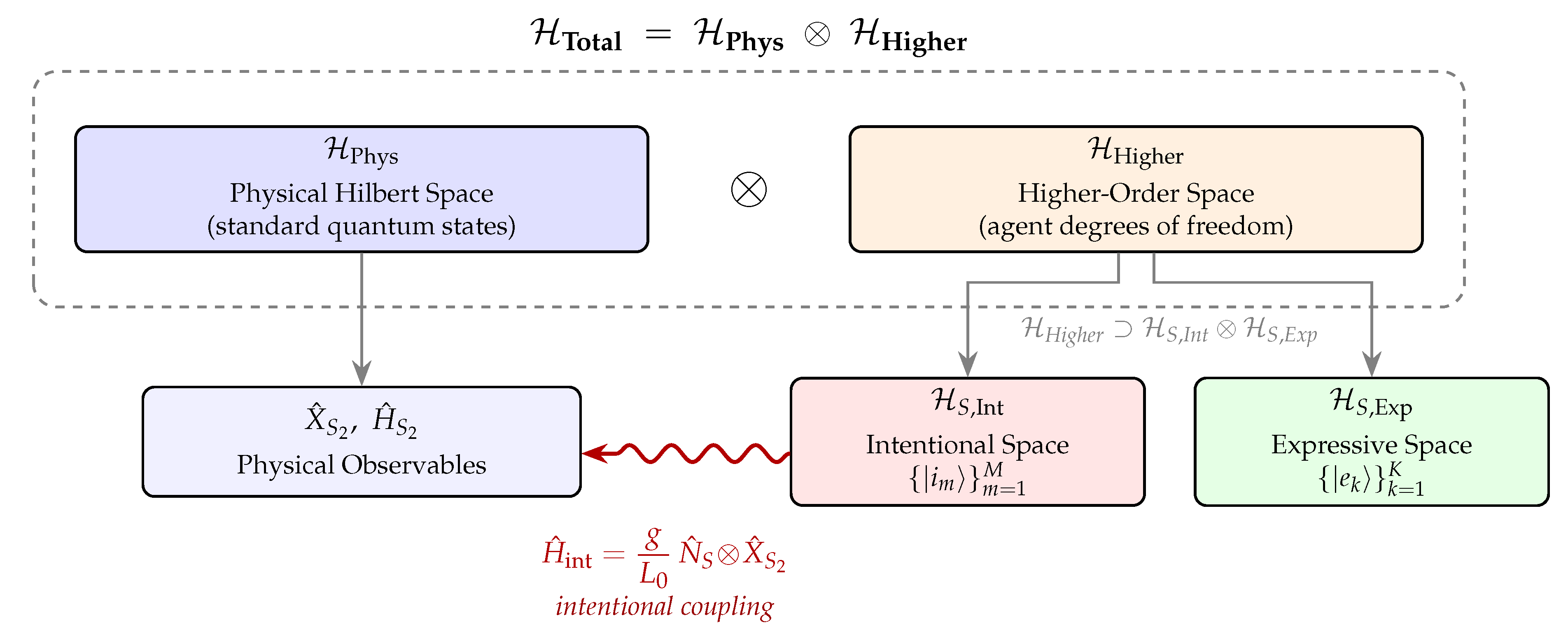
Figure 2.
Mechanism of intentional decoherence in IFT. The full state evolves unitarily in , with the interaction Hamiltonian coupling the agent’s intentional operator to the physical observable . Taking the partial trace over yields the reduced physical state, whose dynamics obey a Lindblad master equation (Theorem 1). The two principal physical predictions—agent-dependent decoherence rate (Proposition 6) and modified Born rule probabilities (Proposition 7)—emerge as consequences.
Figure 2.
Mechanism of intentional decoherence in IFT. The full state evolves unitarily in , with the interaction Hamiltonian coupling the agent’s intentional operator to the physical observable . Taking the partial trace over yields the reduced physical state, whose dynamics obey a Lindblad master equation (Theorem 1). The two principal physical predictions—agent-dependent decoherence rate (Proposition 6) and modified Born rule probabilities (Proposition 7)—emerge as consequences.
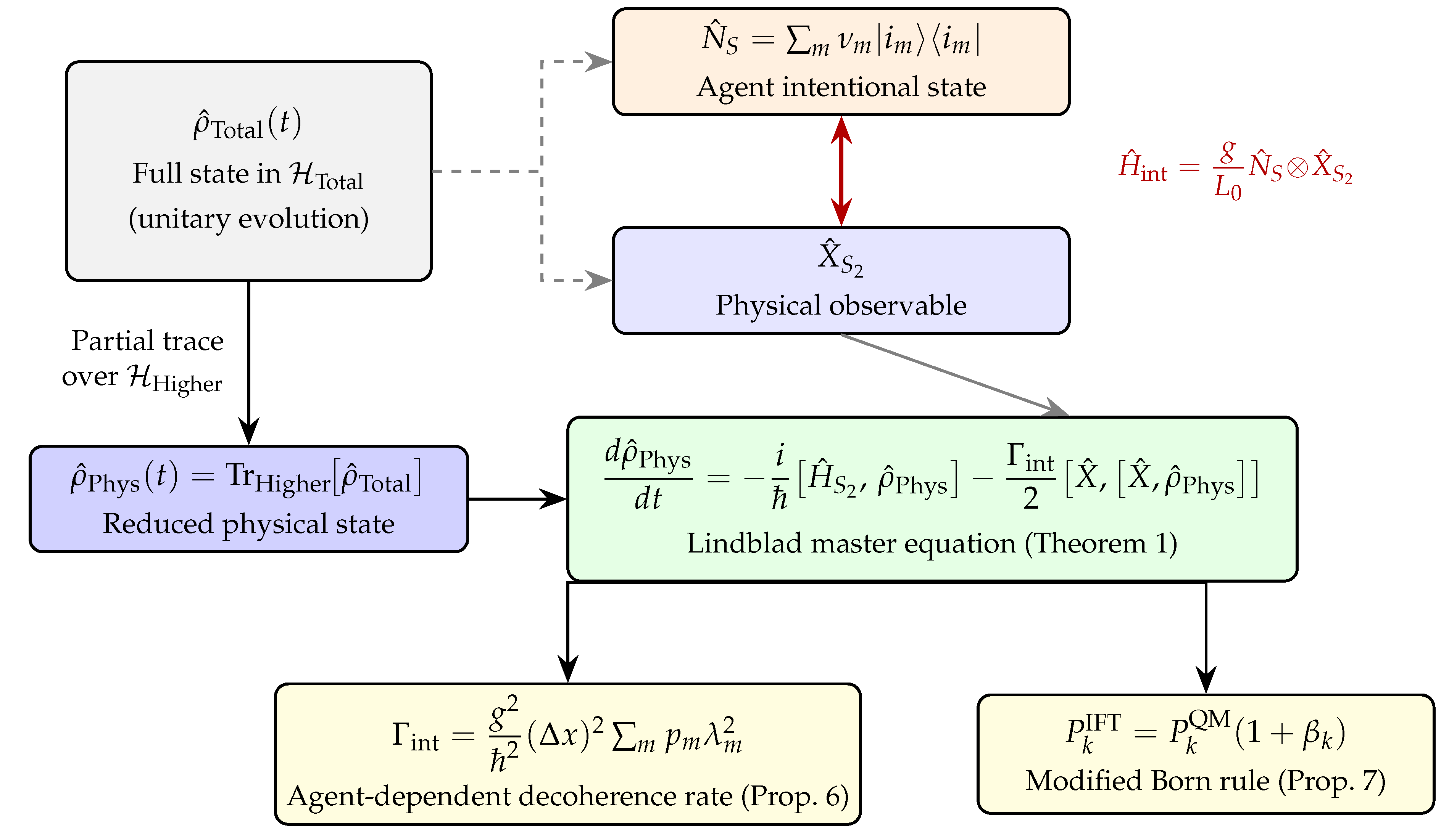
Figure 3.
Schematic of the generic experimental protocol for testing IFT predictions. An intentional agent with characterized state () focuses intention on a quantum system during controlled epochs (Phase 1). The quantum system evolves and is measured with detector efficiency and precision (Phase 2). The observed decoherence rate is compared with the control baseline obtained without an intentional agent (Phase 3). Statistical significance is assessed over N trials at the target SNR. This protocol applies to all ten experimental platforms described in Table 3, Table 4, Table 5 and Table 6.
Figure 3.
Schematic of the generic experimental protocol for testing IFT predictions. An intentional agent with characterized state () focuses intention on a quantum system during controlled epochs (Phase 1). The quantum system evolves and is measured with detector efficiency and precision (Phase 2). The observed decoherence rate is compared with the control baseline obtained without an intentional agent (Phase 3). Statistical significance is assessed over N trials at the target SNR. This protocol applies to all ten experimental platforms described in Table 3, Table 4, Table 5 and Table 6.
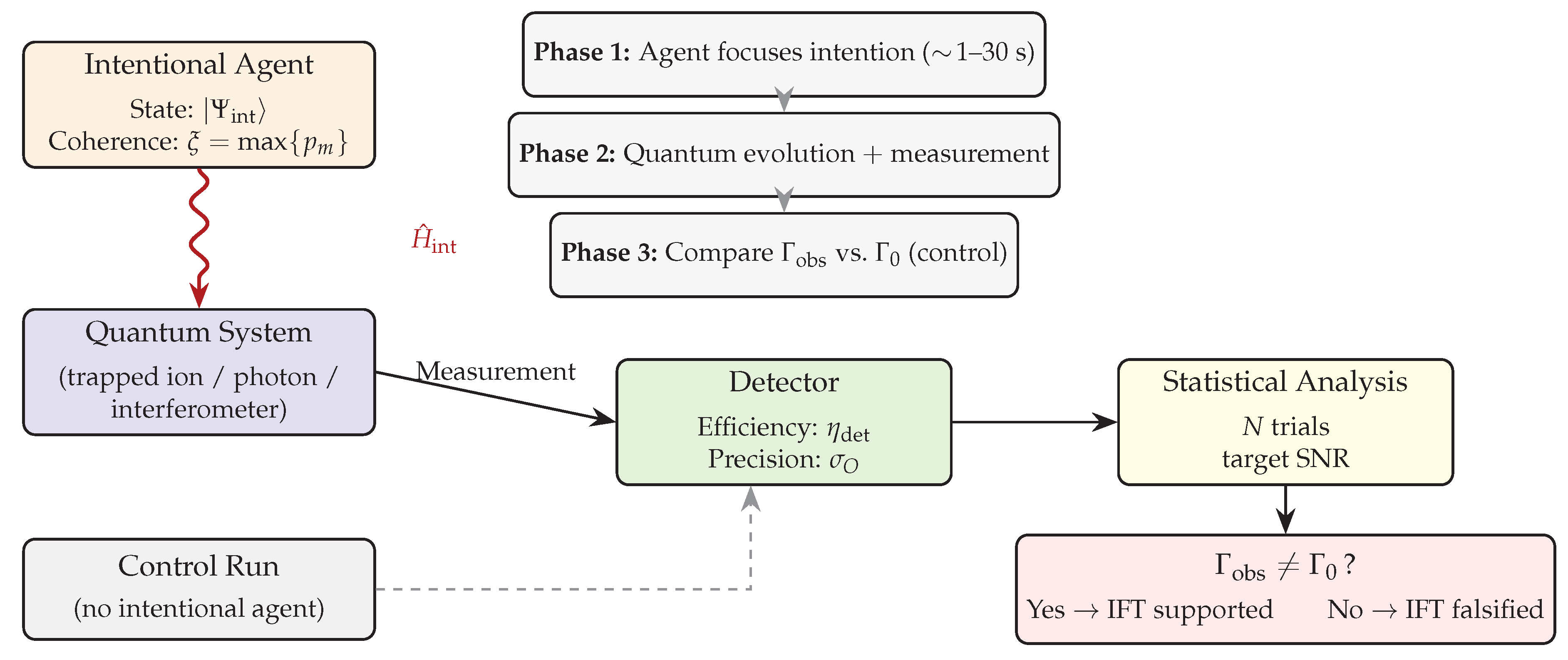
Figure 4.
Decision tree illustrating how major quantum interpretations and IFT address the measurement problem. The tree branches on three key questions: whether collapse is a real physical process, whether it is observer-dependent, and whether a dynamical mechanism is specified. IFT occupies a unique position as the only framework that answers “yes” to all three questions, providing an explicit coupling Hamiltonian and quantitative decoherence rate .
Figure 4.
Decision tree illustrating how major quantum interpretations and IFT address the measurement problem. The tree branches on three key questions: whether collapse is a real physical process, whether it is observer-dependent, and whether a dynamical mechanism is specified. IFT occupies a unique position as the only framework that answers “yes” to all three questions, providing an explicit coupling Hamiltonian and quantitative decoherence rate .
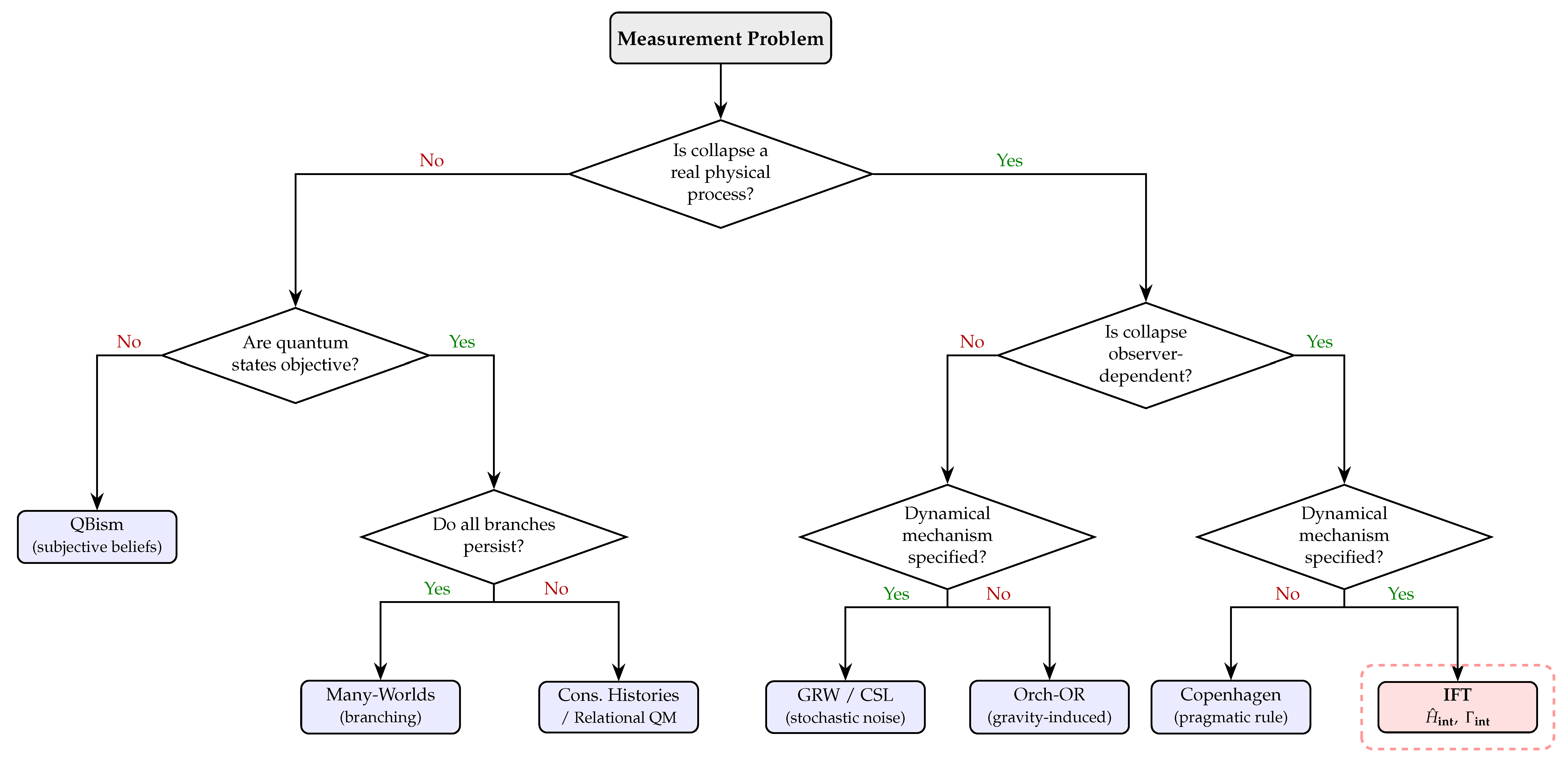

Table 1.
Synoptic comparison of IFT with major quantum interpretations and dynamical models. Key distinguishing features: observer-dependence of collapse/decoherence rates, mechanism for basis selection, and falsifiability beyond standard QM predictions.
Table 1.
Synoptic comparison of IFT with major quantum interpretations and dynamical models. Key distinguishing features: observer-dependence of collapse/decoherence rates, mechanism for basis selection, and falsifiability beyond standard QM predictions.
| Framework | Collapse mechanism | Observer role | Basis selection | Predictions beyond QM | Falsifiable? |
|---|---|---|---|---|---|
| Copenhagen | Postulated | Pragmatic cut | Not addressed | None | No |
| Many-Worlds | No collapse | None (all branches) | Decoherence | None (interpretational) | No |
| de Broglie-Bohm | Effective (guidance eq.) | None | Configuration space | Subquantum nonequilibrium | In principle |
| GRW/CSL | Stochastic (universal) | None | Localization | Mass-dependent collapse rates | Yes |
| QBism | No collapse (subjective) | Central (beliefs) | Agent’s choice | None (interpretational) | No |
| Consistent Histories | No collapse (histories) | Family selection | Consistency condition | None | No |
| Relational QM | Relational | Observer-relative | Not specified | None | No |
| Transactional | Handshake | Transaction trigger | Absorber response | Retrocausal structure | In principle |
| Orch-OR | Gravitational () | Microtubule QC | Gravitational | Mass-dependent | Yes |
| IFT | Intentional () | Dynamical () | Position (Cor. 4) | Agent-dependent | Yes |
Table 2.
Entropic quantification of which-state information extraction across all eleven experiments.
Table 2.
Entropic quantification of which-state information extraction across all eleven experiments.
| Experiment | What information is extracted? | (bits) | (bits) | (J) | |
|---|---|---|---|---|---|
| Quantum Zeno | Which energy level the ion occupies | ||||
| Bomb test | Which path the photon took | ||||
| Which-path (Buks) | Which arm of the AB ring the electron traverses | ||||
| Delayed eraser | Which SPDC path the idler photon followed | ||||
| Before-before | Which polarisation each photon has | ||||
| Wheeler delayed choice | Which path (particle) vs. relative phase (wave) | ||||
| Leggett-Garg | Which macroscopic state the qubit is in | ||||
| Double-slit (Radin) * | Which slit the photon passed through | ||||
| Bell tests | Which spin/polarisation at each station | ||||
| Wigner’s friend | Which outcome the friend observed | ||||
| Matter-wave (Fein) * | Which grating slit the molecule traversed |
Table 3.
IFT predictions organized by observable category with standardized deviation metrics. Within each category the observable type is uniform, enabling direct comparison. : fractional deviation from QM; : estimated signal-to-noise ratio at the stated minimum trial count. All predictions reduce to standard QM when (Corollary 2).
Table 3.
IFT predictions organized by observable category with standardized deviation metrics. Within each category the observable type is uniform, enabling direct comparison. : fractional deviation from QM; : estimated signal-to-noise ratio at the stated minimum trial count. All predictions reduce to standard QM when (Corollary 2).
| Experiment | Observable | Min. trials | ||||
|---|---|---|---|---|---|---|
| Category A: Transition / Detection Probabilities | ||||||
| Quantum Zeno (Itano et al.) | Survival probability | 0.990 | 0.997 | 0.007 | 3.5 | |
| Bomb test (Elitzur-Vaidman) | Interaction-free detection | 0.250 | 0.288 | 0.150 | 3.8 | |
| Category B: Interference Visibility | ||||||
| Delayed choice eraser (Kim et al.) | Coincidence visibility V | 0.050 | 5.0 | pairs | ||
| Wheeler delayed choice (Jacques et al.) | Fringe visibility V | |||||
| Double-slit (Radin et al.) | Spectral ratio | 3.0† | sessions | |||
| Which-path (Buks et al.) | AB visibility | sweeps | ||||
| Matter-wave (Fein et al.) | Fringe visibility V | 0.20 | 0.18 | 0.09 | 4.5 | runs |
| Category C: Correlation / Inequality Measures | ||||||
| Loophole-free Bell (Hensen et al.) | CHSH parameter S | 2.42 | 2.57 | 0.063 | 3.0 | events |
| Before-before Bell (Stefanov et al.) | CHSH parameter S | 2.40 | 2.55 | 0.063 | 3.0 | coincidences |
| Wigner’s friend (Proietti et al.) | Local Friendliness | 2.416 | TBD‡ | sextuplets | ||
| Leggett-Garg (Palacios-Laloy et al.) | LG correlator | 1.50 | 1.53 | 0.020 | 6.0 | trials |
| †Cumulative over ∼250 counterbalanced epochs; ‡Requires aligned-vs-conflicting agent comparison; §Null-background plateau protocol. | ||||||
Table 4.
Standardized intentional agent parameters across experimental platforms. All estimates assume (reduced coupling, Lemma 2). The coherence factor quantifies focused intention quality. Parameters marked “—” are absorbed into the effective .
Table 4.
Standardized intentional agent parameters across experimental platforms. All estimates assume (reduced coupling, Lemma 2). The coherence factor quantifies focused intention quality. Parameters marked “—” are absorbed into the effective .
| Experiment | (IP) | (s−1) | Intention type | Agent class | Number of agents | |
|---|---|---|---|---|---|---|
| Quantum Zeno | 0.8 | 0.95 | Stabilization | Trained | 1 | |
| Bomb test | 1.2 | 0.85 | Detection enhancement | Trained | 1 | |
| Delayed choice eraser | 0.90 | Interference enhancement | Trained | 1 | ||
| Wheeler delayed choice | 1.1 | 0.88 | Wave-like enhancement | Trained | 1 | |
| Double-slit (Radin) | — | 0.90 | Observation focus | Meditator | 1 | |
| Matter-wave (Fein) | 1.0 | 0.90 | (at ) | Decoherence enhancement | Trained | 1 |
| Loophole-free Bell | 1.0 | 0.90 | Correlation enhancement | Trained | 2 (aligned) | |
| Before-before Bell | 1.0 | 0.90 | Correlation enhancement | Trained | 2 (aligned) | |
| Wigner’s friend | — | aligned | Aligned measurement | Trained | 2 (aligned/conflicting) | |
| Which-path (Buks) | 0.8 | 0.90 | 14 (at ) | Observation | Trained | 1 |
| Leggett-Garg | 0.9 | 0.90 | Observation | Trained | 1 |
Table 5.
Practical trade-offs for experimental realization of IFT tests, ranked by estimated feasibility (high to low). Feasibility accounts for platform maturity, achievable precision , trial count N, focus duration, and confound sources.
Table 5.
Practical trade-offs for experimental realization of IFT tests, ranked by estimated feasibility (high to low). Feasibility accounts for platform maturity, achievable precision , trial count N, focus duration, and confound sources.
| Experiment | Precision | Focus duration | Min. trials | Feasibility | Primary confound | Distinctive IFT advantage |
|---|---|---|---|---|---|---|
| Quantum Zeno | s / trial | High | Trap heating | Best ( s−1) | ||
| Leggett-Garg (SC qubit) | s / trial | High | Measurement backaction | Single-system temporal test; | ||
| Before-before Bell | s / block | coincidences | High | Detector efficiency | Two-agent aligned/conflicting test | |
| Loophole-free Bell | s / block | events | High | Event rate (/hr) | Definitive nonlocality baseline | |
| Matter-wave interf. | s / epoch | runs | Medium | Thermal decoherence | Largest () | |
| Bomb test | s / trial | Medium | Dark counts | Largest (15%) | ||
| Delayed choice eraser | s / epoch | pairs | Medium | Alignment drift | High-N statistical power | |
| Wheeler delayed choice | s / epoch | Low | Timing jitter | Retrocausal intentional test | ||
| Wigner’s friend | shift | s / block | sextuplets | Low | 6-photon generation rate | Direct observer-dependence test |
| Which-path (Buks) | s / sweep | sweeps | Medium | Charge noise | Null-background plateau protocol | |
| Double-slit (Radin) | 15–30 s / epoch | sessions | Low | Environmental EMI | Existing data available |
Table 6.
Standardized experimental conditions across proposed IFT test platforms. Operating parameters are reported in a uniform format to enable direct cross-platform comparison. T: operating temperature; : system coherence time; L: characteristic spatial scale of the quantum system; : relevant energy scale; : detector efficiency. Values for proposed IFT tests (Quantum Zeno, bomb test, before-before Bell, Wigner’s friend) are based on state-of-the-art experimental capabilities; values for the Radin double-slit and REG studies are as reported in the original publications.
Table 6.
Standardized experimental conditions across proposed IFT test platforms. Operating parameters are reported in a uniform format to enable direct cross-platform comparison. T: operating temperature; : system coherence time; L: characteristic spatial scale of the quantum system; : relevant energy scale; : detector efficiency. Values for proposed IFT tests (Quantum Zeno, bomb test, before-before Bell, Wigner’s friend) are based on state-of-the-art experimental capabilities; values for the Radin double-slit and REG studies are as reported in the original publications.
| Platform | T (K) | Quantum system | L | Detector | |||
|---|---|---|---|---|---|---|---|
| Trapped ion Zeno | (ion) | 40 / 171 | s | m (trap) | GHz | PMT / EMCCD | |
| SC qubit Zeno | Transmon / fluxonium | s | m (chip) | 5–8 GHz | HEMT amplifier | ||
| Bomb test (MZI) | 295 | Single photons | s (photon) | m (arms) | eV ( nm) | SPAD | |
| Delayed choice eraser | 295 | Entangled photon pairs | s (photon) | m (paths) | eV ( nm) | SPAD | |
| Wheeler delayed choice | 295 | Single photons | s (photon) | m (MZI) | eV ( nm) | APD | |
| Before-before Bell | 295 | Entangled photon pairs | s (photon) | m (arms) | eV ( nm) | SPAD | |
| Wigner’s friend | 295 | 6-photon entangled state | s (photon) | m (paths) | eV ( nm) | SPAD | |
| Double-slit (Radin) | Laser ( nm) | N/A (classical) | m (slits) | eV | 16-bit CCD | ||
| Loophole-free Bell | 4 (NV) / 295 | NV− spins / photons | s (NV) | km (Delft) | eV ( nm) | APD ( eff.) | |
| Matter-wave (KDTLI) | (source) | Oligoporphyrins (25 kDa) | ms (transit) | nm (gratings) | eV (thermal) | QMS / ionization | |
| Which-path (AB ring) | GaAs 2DEG electrons | ns | m (ring) | meV () | QPC current | ||
| Leggett-Garg (SC) | Transmon qubit | s | m (chip) | 5–8 GHz | HEMT amplifier | ||
| REG (PEAR) | Zener diode noise | N/A (classical) | N/A | 5–8 V bias | ADC |
Disclaimer/Publisher’s Note: The statements, opinions and data contained in all publications are solely those of the individual author(s) and contributor(s) and not of MDPI and/or the editor(s). MDPI and/or the editor(s) disclaim responsibility for any injury to people or property resulting from any ideas, methods, instructions or products referred to in the content. |
© 2026 by the authors. Licensee MDPI, Basel, Switzerland. This article is an open access article distributed under the terms and conditions of the Creative Commons Attribution (CC BY) license (http://creativecommons.org/licenses/by/4.0/).
Copyright: This open access article is published under a Creative Commons CC BY 4.0 license, which permit the free download, distribution, and reuse, provided that the author and preprint are cited in any reuse.