

Submitted:
22 May 2026
Posted:
25 May 2026
You are already at the latest version
Abstract
The Klamath-Siskiyou Ecoregion (KSE) of southwest Oregon-northern California, USA has globally exceptional biodiversity but is experiencing mounting pressures from climate change and land uses. We conducted an ecoregional conservation assessment of the KSE and the Siskiyou Crest subregion (SCS), a proposed climate refugium within the KSE, to integrate protected area priorities with climate change planning and fire risk reduction for communities. Both areas contained very low levels (<30%) of protection (GAP status 1, 2) for nearly all land cover types (n=22), including serpentine substrates where endemic plants are highly concentrated, older forests with potential refugia properties, and habitat for Northern Spotted Owl (Strix occidentalis caurina) and Pacific fisher (Pekania pennanti). At the ecoregional scale, high severity fire levels were proportionately similar across GAP land-use status (“managed” vs. protected). However, high severity fire was lowest for protected areas at the subregional scale reflective of potential refugium properties. Most fuel treatments by federal agencies were >1-km from nearest structures, far removed from effective community fire protection in both locales. The relatively higher-elevation SCS is projected to maintain refugia properties (cooler, wetter) for longer periods than the KSE; however, that function may dissipate toward the end of the century and under a higher emissions scenario. Stepped up protections especially of potential refugia combined with fire risk reduction of the built environment are urgently needed to prevent unprecedented losses.
Keywords:
biodiversity
; climate change
; climate refugia
; ecoregion
; globally outstanding
1. Introduction
Reserve design is the hallmark of conservation biology approaches that typically include representation of landforms, focal species, or vegetation types in large, interconnected protected areas [1]. Such approaches are essential for ameliorating the global extinction crisis through global protected area targets (e.g., 30 percent protected by 2030, “30 x 30”, [2]).
Ecoregional conservation assessments (ECAs) are a means for meeting conservation targets by developing integrated strategies that address climate change and land-use impacts [3]. ECAs include spatially explicit analyses of select ecosystems and focal species overlaid on land-use categories using the U.S Geological Survey Protected Areas Database (PAD) to determine gaps in protected area coverages. They include climate change downscaling to assess future risks to biodiversity and identify potential refugia for protection. Such an ECA methodology was piloted for the Mogollon Highlands Ecoregion of Arizona to New Mexico, including identifying the Gila Bioregion as potential refugium [4]; the Southern Rockies Ecoregion of Wyoming to New Mexico, including Santa Fe, New Mexico watersheds as potential refugia [5]; and the Northern Rockies Ecoregion of Washington to Montana, including the Yaak Valley watershed as potential refugium [6]. ECA approaches can assist governments and conservation groups in prioritizing protected area additions that might provide time for species to adapt to the unprecedented pressures of land-use changes and climate change.
The Klamath-Siskiyou Ecoregion (KSE) of southwest Oregon and northern California has a history of conservation interests due to it is widely recognized biodiversity importance [1,7,8,9], including recognition as a World Wildlife Fund “Global 200 Ecoregion” [10]. The KSE is considered a “center of floristic diversity and narrow endemism” [8]. The ecoregion supports a continental maximum of conifer species [11] along with exceptional mollusk (Mollusca); butterfly (Lepidoptera); bee (Apidae) [12]; and amphibian richness and endemism ([9,13] for reviews). Notably, the KSE has the most species-rich herpetofauna of any similarly sized mountain range in the Pacific Northwest, in part, due to eight endemic species [14]. Plant endemism on ultramafic substrates is exceptional, promoted by the combination of extensive serpentine areas and a moderate inland to coastal climate [15].
The KSE also has presumed refugia properties related to its moderate climate [7,9,16], and the lack of volcanic activity and glaciation events. Olson et al. [17] identified old forests on north-facing slopes as potential refugia presumably because of favorable microclimatic properties (cool, wet). The primarily east-west running, high-elevation, Siskiyou Crest Subregion (SCS) within the KSE, is also noted for its biodiversity and forest carbon importance that is greatest in older forests [18], along with its land-bridge functions connecting the Cascade and Coast ranges [17]. This subregion has been proposed for protection by conservation groups (https://siskiyoucrestcoalition.org/; accessed May 8, 2026) that requested an ECA to help align protected area strategies with presumed refugium properties of the Crest. Moreover, this ECA updates prior conservation planning in the KSE [1].
Main climate stressors in the KSE include increases in extreme temperatures, more frequent droughts, insect outbreaks, and wildfires [19,20]. Such changes may impact moisture dependent taxa (e.g., salamanders, mollusks) [9,17], endemic plants with restricted ranges and “relict” populations [21], and species that use older forests as wildfire [22] and climate refugia [23]. Additionally, logging, roads, mining, off-highway vehicles, and livestock grazing are cumulative stressors impacting large portions of the KSE [9,24,25]. Such stressors may interact with climate change to accelerate biodiversity loss (e.g., logging x extreme fire weather [26]).
We provide a multi-scaled ECA for the KSE and the SCS that is based on representation analyses of select ecosystems and focal species in relation to specific conservation targets, including 30% protected by 2030 (i.e., “30 x 30” [2], herein low target), 50% protected by 2050 (i.e., “50 x 50” [27], herein intermediate target), and 100% protected (no timeline, herein upper target) of select types. The upper bound (100%) target is focused on older forests [28,29] and federally Inventoried Roadless Areas (IRAs) due to their importance [30]. We also chose the Pacific fisher (Pekania pennanti) and Northern Spotted Owl (Strix occidentalis caurina, a federally threatened species; NSO) as focal species because of their association with older forests [31,32].
We also examine wildfire severity in relation to land-use categories (i.e., GAP status, see below) mainly because protected area proposals have frequently been blocked by decision makers over concerns about wildfires spilling into urban areas with management responses aimed at unprecedented increases in fire suppression and various forms of logging, road building, and prescribed burning (slash pile and prescribed fire) (e.g., the Fix Our Forests Act H.R. 471 see https://www.congress.gov/bill/119th-congress/house-bill/471; accessed April 24, 2026 and numerous land management forest planning documents). Thus, we integrate conservation priorities with wildfire risk reduction for communities living in the so-called wildland-urban interface (WUI) as defined by federal agencies. Like in the other ECAs, our findings may be exportable to other ecoregions facing similar stressors that require integrated conservation strategies.
2. Materials and Methods
2.1. Study Area
The ~4.83M ha KSE spans the Klamath and Siskiyou Mountains of southwest Oregon and northern California (Figure 1). We used the U.S. EPA Level III Ecoregion (#78, Klamath Mountains/California High North Coast Range, L3 Code:6.2.11) to define the study area. This ecoregion dataset was originally derived from Omernik [33] and from mapping done in collaboration with U.S. EPA regional offices, federal agencies, state resource management agencies [34]. There are some boundary differences with the WWF Global 200 Ecoregion #39 (Klamath-Siskiyou Forests), which spills over into portions of coast redwood (Sequoia sempervirens) and includes more watersheds at the northern boundary of the KSE. Our KSE map is also like Bailey’s [35] Klamath Mountains and Southern Cascades (M261A, M261D), however, Bailey also included portions of the Cascades not included in our map (see [10] for comparisons of ecoregional boundaries).
The KSE is considered to have “central significance” [8] in adjoining the Coast Range Ecoregion to the west, the Southern and Central California Chaparral and Oak Woodlands Ecoregion to the south, the Cascades and Eastern Cascades Slopes and Foothills Ecoregions to the east, and Willamette Valley Ecoregion to the north [36].
Notably, the 697,755 ha SCS (14.5% of the KSE) is the only high-elevation land bridge (east-west) in the ecoregion (Figure 1). Original mapping of the SCS provided by the Siskiyou Crest Coalition (local conservation groups) had identified the upper elevation land-bridge. Their mapping included watersheds intersecting the Siskiyou Crest and the geographically distinct land masses and boundaries that note the convergence of the Klamath-Siskiyou Mountains with the Cascade Mountains and Coast Ranges of California and Oregon (https://siskiyoucrestcoalition.org/; accessed May 4, 2026). The SCS also contains the watershed divide between the Klamath and Smith and Klamath and Rogue watersheds (see Figure 1) and has local significance as the 1850s “State of Jefferson” that demarked the large mountain range dividing Siskiyou County, California from southwestern Oregon. The boundaries of the region thus include the Coast Range and Middle Fork Smith River to the west, the Cascade Mountains to the east of Siskiyou Summit, the Rogue and Illinois River Valley's to the north in Southwest Oregon and the north bank of the Klamath River from Cottonwood Creek downstream to Blue Creek.
Using a continental dataset of multiple taxa, Ricketts et al. [10] (Appendix C) reported that the KSE supports 1,859 vascular plant species with up to 150 plant endemics. DellaSala et al. [9] identified several distinctive, rare and imperiled taxa in the KSE. Kauffmann and Garwood [11] listed 35 conifer species, which is considered globally significant among temperate conifer forest regions [9]. Several conifers are considered to have relict populations (i.e., more common in a different geological period but restricted today) [37]. Some conifers also have range extensions mainly on cool, moist slopes including Alaska yellow cedar (Callitropsis nootkatensis, relict populations), Pacific silver fir (Abies amabilis, relict populations), subalpine fir (Abies lasiocarpa, relict populations), Engelman spruce (Picea engelmannii, relict populations), and noble fir (Abies procera). Others conifers have range extensions on hot, dry slopes, including western juniper (Juniperus occidentalis), foxtail pine (Pinus balfouriana, relict species), and gray pine (Pinus sabiniana) [11,38]. Additionally, three conifer species are endemic to the KSE, including Brewer spruce (Picea breweriana) (relict populations), Baker’s cypress (Hesperocyparis bakeri), and Port Orford cedar (Chamaecyparis lawsoniana) [11]. The KSE also overlaps with the northern extension of the California Floristic Province, a recognized global biodiversity hotspot [39]. In sum, the diverse geological, topographic, and climatic processes in the KSE have resulted in zonal vegetation considered more complex than the nearby Sierra Nevada and Cascade ranges [16].
Older forests of the KSE have multi-layered canopies characterized by tall evergreen needleleaf trees overtopping evergreen broadleaf and sclerophyllous vegetation [8] that ostensibly confer fire-resistant properties as refugia [40,41]. Xeric sites are dominated by Douglas-fir (Pseudotsuga menziesii) and ponderosa pine (Pinus ponderosa) mixing with a rich assortment of oak (Quercus spp.) woodland and chaparral [11]. Upper elevations are dominated by firs (Abies spp.).
Climatic conditions in the KSE are generally Mediterranean with wet, cool winters and dry, warm summers (e.g., Koppen climate classification Csb [42]) characterized by steep climatic gradients from the coast (wet, fog, cool) to inland (dry, warm) and from low (seasonal rain) to upper elevations (snow) (see Table 9.1 in Skinner et al. [16] for temperature and precipitation figures). Wet and dry alternating climatic cycles, and therefore fire activity, are on long timelines in relation to the Pacific Decadal Oscillation [43]. Fires tend to produce mixed severity effects on plant communities characterized by large and small patches of low, moderate, and high severity [44] that support exceptional biodiversity. Fires more prevalent during the pre-fire suppression era and localized fires set by Indigenous peoples [16]. Fires also tend to be more naturally (unaided) prevalent at low elevation, xeric sites (especially south slopes) vs. longer fire return intervals in mesic and upper elevations [16].
Contemporary wildfires are increasingly driven by extreme fire weather [20] interacting with heavily logged landscapes [26,40] that result in fast-moving wildfires that can spill over into towns juxtaposed with wildlands [45]. High road densities in the KSE [24] add to wildfire risks from unwanted human-caused ignitions [46,47]. Additionally, reoccurring high severity fires have functioned as a self-perpetuating process for rejuvenating fire-dependent sclerophyllous plants mainly on south-facing and xeric environments [48]. The KSE has also experienced overlapping short interval (<20 years), high severity fires in forests, which despite repeat stand replacing events, still contain plant species characteristic of pre-fire events [49]. There is also high taxa richness in the ensuing complex early seral forests [50], including high bird [51] and small mammals [52] richness with the latter providing prey for species that hunt in open, shrubby areas and nest in unburned (or low severity) old forest patches (fire refugia) such as NSO [53]. However, others have reported the potential for type conversions of conifers to hardwoods if the interval between high severity fires is further reduced by climate change [54] or unplanned and frequent wildfire ignitions [47].
2.2. Mapping Methods
We generally followed the methods outlined in DellaSala et al. [6]. We obtained GIS data from a variety of sources (Figure 2), reprojected to a CONUS Albers projection (EPSG:5070) and clipped geospatial datasets to the study area using QGIS version 3.44. For any of our GAP representation analyses, we rasterized vector datasets using a 30m grid aligned with LANDFIRE (2024, LF 2.5.0) rasters. All clipped and reprojected rasters we used in our GAP representation analyses therefore had the same parameters except for pixel values. We stacked these rasters into a multiband virtual raster using the Geospatial Data Abstraction Library (GDAL) in Python 3.11.14. We then used the rasterio, pandas, and numpy Python libraries to parse the virtual raster data, calculate the area for each unique combination of stacked pixel values, and store results in a SQLite database. We used pandas and the sqlite3 library to perform a series of SQL queries on our SQLite database from within Python and create summary tables across all our metrics except those used in our fuels and WUI analyses and our climate change analyses. All maps, except those in our climate change analyses, were created in QGIS 3.44.
2.3. Topography and Hydrography
We obtained elevation and aspect data from LANDFIRE. For elevation, we created six 500-m bins, with the highest elevation bin being > 2500 m. We grouped degrees aspect into five standard categories: flat, north, east, south, and west. For watersheds, we obtained Hydrologic Unit Code (HUC) 6 and 8 polygons from the United States Geological Survey (USGS) Watershed Boundary Dataset. While we conducted a GAP distribution analysis across all watersheds at both scales, we were most interested in analyzing HUC6 watersheds at the KSE scale and HUC8 watersheds at the SCS scale.
2.4. Land Ownership/Management and GAP Status
We used the PAD (PAD-US 4.0, [55]) to determine land ownership or management entity across the study area. We consolidated land management entities into seven groups (Figure S1).
We used similar methods to DellaSala et al. [4,5,6] and extracted USGS Gap Analysis Project (GAP) status codes 1-4 from the PAD. GAP 1 is assigned to lands managed for biodiversity, where disturbance events proceed or are mimicked (e.g. federally designated Wilderness areas). GAP 2 is assigned to lands managed for biodiversity, but where disturbance events are suppressed (e.g., national monuments). GAP 3 is assigned to lands managed for multiple uses and may be subject to extraction such as mining or logging as well as livestock grazing and off-highway vehicle use (e.g. non-Wilderness national forest lands). GAP 4 is assigned to lands with no known mandate for biodiversity protection (e.g. private lands). We considered both USDA Forest Service designated and managed Inventoried Roadless Areas (IRAs) and U.S. Department of Interior Bureau of Land Management (no date) “Lands with Wilderness Characteristics” (LWCs) that the agency has identified as managed “to protect” to have enhanced protection beyond what is usually assigned GAP 3 status. We therefore split GAP 3 into GAP 3a and GAP 3b, assigning IRAs and select LWCs (that are managed “to protect”) a status of 3a and all other GAP 3 lands a status of 3b. We consider lands with a status of either GAP 1 or 2 to be “protected” and lands with a status of either GAP 1, 2, or 3a to be “protected+” to identify which landscapes meet 30x30 or 50x50 targets both with and without IRAs and select LWCs. IRA polygons were obtained from the PAD while LWC polygons were obtained for the Oregon portion of the KSE from the U.S. Department of Interior Bureau of Land Management [56]. We did not include LWC polygons from the California portion of the KSE as those GIS data, if they exist, are not publicly available. Modified GAP status is depicted for the entire KSE and SCS in Figure S2.
2.5. Land Cover
For vegetation types, we used LANDFIRE Biophysical Settings (BPS) combined with agricultural and developed vegetation types from the LANDFIRE (2024, LF 2.5.0) Existing Vegetation Type (EVT) dataset. Based on initial comparisons of EVT data to high-resolution satellite imagery across post-fire landscapes in our study area, we determined that BPS would be a better representation of vegetation types in the study area. Disturbances such as moderate and high severity fire can significantly change EVT classification for a given area. For example, many mixed-conifer forests that experience high severity fire are subsequently classified as shrubland in the EVT dataset, likely due to a change in canopy structure. However, these areas may still be naturally regenerating as part of a post-fire succession process that will eventually result in a return of mature mixed-conifer canopy. We therefore did not want to classify complex early seral forest (CESF) [50] as non-forest vegetation types when analyzing protection levels. BPS is not sensitive to natural disturbances like EVT, but it also does not account for areas that have been converted to agricultural use or any type of development. To effectively leverage the long-term natural vegetation classification stability of BPS while still accounting for agricultural or developed lands, we combined the two datasets and kept BPS vegetation types except where they intersected agricultural and developed EVTs, in which case we retained the EVTs. We then organized these modified BPS vegetation types into 22 broader categories (see Table S1) that represent consolidated forest types, shrubland, grassland, and other land covers similarly to DellaSala et al. [5,6]. This allowed us to simplify our GAP representation analyses across vegetation types.
2.6. Late-Successional and Old-Growth Forest Distribution
We obtained late-successional and old-growth forest distribution spatial data from the Northwest Forest Plan Monitoring Program’s annual old-growth structure index (OGSI) [57] and GIS datasets [58]. OGSI data use two age thresholds: >80 years but < 200 years (herein, OGSI 80) indicates late-successional (mature) forests; >200 years (herein, OGSI 200) indicates old-growth forests. Annual data for the entire KSE were available from 1986 to 2024. These raster datasets included four contiguity categories for each OGSI age threshold: core, edge, finger, and scatter. For our analyses, we consolidated these contiguity categories into a single class.
We only used data from 1986 and 2024 for our analyses. The 2024 data were used for GAP analyses of “current” OGSI distribution across the study area. We also analyzed GAP representation across each OGSI age threshold that persisted from 1986 to 2024 despite experiencing at least one fire (see section 2.8 below for methods on fire data collection). That is, if a cell in our raster grid was identified as OGSI 80 in both 1986 and 2024, and it burned in at least one wildfire from 1986 to 2023, it was considered to have “persisted.” We also analyzed GAP representation of areas that shifted from OGSI 80 to OGSI 200 between 1986 and 2024 (“promoted”) despite burning in at least one fire. We did not consider fires that burned in 2024 for these persistence and promotion analyses as our inspection of the spatial data indicated that most fires did not affect the OGSI data until year after the fire. For example, a large high severity fire patch occurring in 2020 would not appear as a loss of OGSI 80 or 200 until the 2021 OGSI datasets. Therefore, 2024 OGSI data would only reflect fires that occurred up to 2023.
2.7. Focal Species Suitable Habitat and Serpentine Areas
We held an expert’s workshop in August 2024 to identify conservation priorities for analysis and compile information on taxa that might benefit from presumed refugia in the KSE and the SCS. At the workshop, we chose focal taxa based on habitat associations with old forests and availability of published datasets that fit the multi-scaled analysis.
For NSO, we collected habitat suitability data from the Northwest Forest Plan Monitoring Program (similarly to OGSI data), which were available as annual rasters from 1986 to 2024 [59]. NSO habitat data were classified into unsuitable, marginal, suitable, and highly suitable. We analyzed only the GAP status distribution for suitable and highly suitable habitat in 1986 and 2024 that persisted despite experiencing at least one fire through 2023.
For Pacific fisher, we analyzed GAP status distribution for the entire study area for the Connectivity Conservation Priority Areas [60], which used habitat suitability models to delineate core areas and least-cost corridor models to identify linkages among them.
We also used a serpentine geology dataset that was manually digitized by Noss et al. [1] using 1:500,000 USGS geology maps for both Oregon and California and spanning our entire study area.
2.8. Fire Severity
We collected fire perimeter and fire severity data from the Monitoring Trends in Burn Severity (MTBS) database only available from 1985 through 2023. We limited our analyses to fires categorized as wildfire, wildland fire use, and unknown—we did not include prescribed fire. We used the relativized delta normalized burn ratio (RdNBR) dataset for each fire and classified RdNBR into unprocessed (i.e., areas that had no RdNBR values due to cloud cover or satellite image collection issues), unchanged, low, moderate, and high severity fire according to established thresholds [61]. We then mosaicked these RdNBR class data by year. These annual mosaics allowed us to calculate the number of fires a given location in our study area experienced over the study period. We also combined all annual mosaics into a single fire severity footprint dataset, where the highest fire severity a cell in our raster grid experienced over the study period was retained. We then analyzed the GAP status distribution across each fire severity class footprint. We conducted this analysis once for all land cover categories combined and then again for only the more frequent fire, drier forest types found in the KSE: dry Douglas-fir Forest and woodland, dry mixed conifer forest and woodland, mesic mixed conifer forest and woodland, and ponderosa pine forest, woodland and savanna.
2.9. Fuel Treatments and the Built Environment
Most public land in the study area is managed by either the USDA Forest Service or the Bureau of Land Management (Figure S1). As in our previous ECAs [5,6], we analyzed the location of fuel treatments in relation to the WUI. We obtained WUI data from Radeloff et al. [62] by extracting low, medium, and high-density wildland-urban interface and intermix polygons similarly to [5,6]. We considered any land within these six categories to be WUI. We also created buffers around WUI areas in 250-m increments up 1000 m. We collected fuel treatment data from the USDA Forest Service’s Hazardous Fuel Treatment Reduction (polygon) dataset [63] and the Bureau of Land Management’s Historical Fuels Treatment Polys dataset (itself pulled from the National Fire Plan Operations and Reporting System) [64] from the last 20 years of our study period (2005-2024). We selected this date range for our analysis as we were primarily interested in contemporary fuel treatment patterns and because pre-2005 fuel treatment data were limited. We filtered the large, national datasets for each agency to only treatments with actual completion dates between 2005 and 2024 and with an activity or type name of chipping, crushing, mastication, mastication/mowing, broadcast burn, jackpot burn, machine pile burn, and thinning, and then clipped them to the KSE. Each agency’s dataset also has information about whether the agency classified the treatment polygon as WUI (i.e., a true/false field called “IsWui” or “ISWUI”). For each agency we dissolved all treatments by the agency’s WUI classification and then intersected these dissolved treatment polygons with the 250-m WUI buffers. Any treatment polygons or portions of polygons outside of the WUI buffers was assigned a WUI distance of >1000 m. We did this at both the KSE and SCS scale and calculated the total hectares and percentages of treatments at each buffer distance and the proportions of these areas considered WUI or not WUI by the respective agency.
2.10. Climate Change
We used the global climate model (GCM) output from phases 5 and 6 of the Coupled Model Intercomparison Project (CMIP) for climate projections [65,66]. These two modeling efforts established common future climate scenarios under which all global climate models were forced. Climate scenarios for CMIP5 are called representative concentration pathways, or RCPs while for CMIP6 we updated the scenarios to shared socio-economic pathways, or SSPs. RCPs from the CMIP5 models are roughly comparable to the SSPs from CMIP6 except they now have socio-political narratives attached to each scenario. For both CMIP5 and CMIP6-based future climate projection data, we selected both an “intermediate” future scenario (RCP 4.5 and SSP245) and a “very high” future scenario (RCP 8.5 and SSP585). We refer to RCP 4.5 and SSP245 scenarios as “intermediate” and the RCP 8.5 and SSP585 scenarios as “very high” due to their relative amounts of greenhouse gas emissions and to maintain consistency with international climate reports [67,68].
Raw GCM projection output from the CMIP models have resolutions that are typically greater than 1°latitude x 1° longitude. Because the data are so coarse, it is difficult to interrogate the data for meaningful information at regional scales, like ecoregions. To make the data more relevant for regional scale assessments, we “downscaled” climate data to a finer resolution through statistical and dynamical downscaling. Statistical downscaling uses empirical relationships and statistical methods to interpolate data to a higher resolution, and dynamical downscaling uses a regional climate model forced by the GCM data to create a dataset with higher resolution. For several of the climate indicators assessed in this study, we used GCM data that have been statistically downscaled by the localized constructed analogs method version 2, which we hereafter refer to as LOCA2 data [69].
The LOCA2 method uses empirical relationships between large-scale atmospheric climate patterns and on-the-ground conditions to bias-correct the global climate model output. Other indicators require dynamical downscaling due to not being a direct output from global climate models; namely, indicators that are related to hydrology, like snowpack. For the snowpack indicator, we used hydrologic projections from the Variable Infiltration Capacity (VIC; [70]) model forced by a statistically downscaled global climate model dataset. The statistically-downscaled dataset is the Multivariate Adaptive Constructed Analogs version 2– Livneh dataset [71], which uses data from Livneh et al. [72] to train the statistical downscaling method. Finally, to better understand future wildfire conditions, we used output from the MC2 regional vegetation model [73]. The LOCA2 data uses the CMIP6 future climate scenarios (SSPs) and the MACAv2-Livneh and MC2 wildfire projections use the CMIP5 future scenarios (RCPs).
3. Results
3.1. Representation Analyses
3.1.1. Topography and Hydrography
Protected areas are highly skewed toward upper (>1500 m) elevations in the KSE but not as much as in the SCS that had low levels of protection across all elevations (Figure 3). Notably, IRAs and select LWCs are also skewed toward upper elevations (>1500 m) in both areas (orange color).
There are 35 HUC8 watersheds within the KSE and seven HUC8 watersheds within the SCS (Table S2). For the KSE, six HUC8 watersheds met at least the lowest target (Chetco, Middle Fork Eel, Salmon, Smith, Trinity, Upper Cache) with four additional watersheds (Cottonwood Creek, Illinois, Lower Klamath, and McCloud) meeting at least the lowest target with the inclusion of protected+. Notably, the Salmon HUC8 watershed approaches 70% under protected+. For the SCS, only one of the HUC8 watersheds (Smith HUC8) met the lowest target with the addition of the Lower Klamath meeting the target if protected+ is included (Table S2).
3.1.2. Land Ownership/Management
Approximately one-half to two-thirds of the KSE and SCS, respectively, is under the management of the USDA Forest Service where there are opportunities for large-scale conservation (Table 1). There are some large contiguous GAP 1 areas across the region (Figure S2), but overall protection levels are still well below the lowest target with only 15% and 14.5% protected for the KSE and SCS, respectively. Protected+ would approach 25% protected for both areas, which is still below the lowest target.
3.1.3. Land Cover
We mapped 71 modified BPS land cover types in the KSE and 44 in the SCS (Table S1) that were then consolidated into 22 broader categories for the representation analysis (Table 2 and Figure S3). Mixed conifer forest and woodland (both dry and mesic) comprise 48.3% of the KSE and 50.1% of the SCS, and California mixed evergreen forest and woodland account for 16.9% and 26.2% of the KSE and SCS, respectively.
Of the 22-land cover categories, only five met the 30% conservation target in the KSE (Table 2). Upper elevation categories, including perennial ice/snow, red fir forest, and subalpine forest and woodland are more than 50% protected (Table 2) due to substantial proportions of these landscapes within federally designated Wilderness areas across the KSE. Including protected+ would boost protection levels across most categories; however, only mesic mixed conifer forest and woodland would be elevated enough to meet the 30% conservation target (shifting from 27% to 38.5%; Table 2).
For the SCS, only four of the subgroups met the conservation target, though one of these was open water (Table 2). Protected+ would improve representation levels for most categories, elevating three categories to the 30% conservation target: red fir forest (shifting from 14.4% to 47.2%), riparian and wetland (27% to 38.4%), and subalpine forest and woodland (21% to 47.8%).
Notably, 580,507 ha of serpentine, where plant endemism is exceptionally high, exists within the KSE; however, only 24% of it is protected (see Figure S4 and Table S3). The addition of protected+ would bump up representation targets to >40% (Table S3). The SCS includes 130,649 ha of serpentine with only 26% protected; protected+ would boost overall protection levels to 40% as in the KSE (Table S3).
3.1.4. Late-Successional and Old-Growth Forest (LSOG)
The KSE contains ~1.85M ha of OGSI 80 and ~896K ha of OGSI 200, while the SCS contains ~348K ha of OGSI 80 and ~195K ha of OGSI 200 (Table 3, Figure 4). Notably, the SCS stands out as having a high concentration of OGSI 80 and 200, particularly in the southern portion (Figure 4). In fact, while the SCS accounts for only 14.5% of the KSE land area, it contains 18.8% and 21.8% of all OGSI 80 and 200, respectively, in the ecoregion.
We also analyzed the subset of late-seral forests that have persisted from 1986 to 2024 despite burning in at least one fire event from 1985-2023. The KSE and SCS respectively contain 603K ha and ~101K ha of persisted OGSI 80 (Table 3). And while only 18.3% of OGSI 80 in the KSE was in protected areas, these GAP 1 or 2 areas contained almost 34% of persisted OGSI 80. Similarly, 17.6% of OGSI 80 in the SCS was in protected areas while these areas contained 35.1% of persisted OGSI 80 (Table 3).
There are nearly 297K ha and 55,459 ha of late-seral forest that was OGSI 200 in 1986 and stayed OGSI 200 in 2024 despite burning in at least one fire in the KSE and SCS, respectively (Table 3). About 21% of OGSI 200 in the KSE was found in protected areas compared to 34.1% of persisted OGSI 200 found in these areas. And nearly 19% of OGSI 200 in the SCS was in protected areas compared to 34.7% of persisted OGSI 200.
Lastly, there are 364K ha and 65,411 ha of late-seral forest that was OGSI 80 in 1986 and developed (promoted) into OGSI 200 by 2024 despite experiencing at least one fire from 1985-2023 in the KSE and SCS, respectively (Table 3). These areas accounted for 40.7% of all OGSI 200 in the KSE and 33.5% in the SCS. And 34.2% of these promoted areas were in protected areas in the KSE, about 35% in protected areas in the SCS. Notably, a substantial proportion of OGSI 80, persisted OGSI 80, promoted OGSI, OGSI 200, and persisted OGSI 200 was in GAP 3a areas (protected+, ranging from 11.3 – 18.9%) in the KSE, a pattern that was even more prevalent in the SCS (13.9 – 22.8%; Table 3).
3.1.5. Focal Species
The KSE contains 1.23M ha of NSO suitable (~40%) and highly suitable (~60%) habitat while the SCS contains 291K of suitable (39%) and highly suitable (61%) (i.e., similar proportions; see Table 4 and Figure S5). The KSE also contains 308K ha of NSO habitat that persisted (as either suitable or highly suitable) from 1986 to 2024 despite burning at least once between 1985 and 2023, with 28.9% of this persisted habitat in protected areas and nearly 50% within protected+ (Table 4). Another 60K ha of NSO habitat persistence occurs in the SCS with most (62%) in the highly suitable layer and just over 30% of that protected. Protected+ would boost levels to near the intermediate target for the KSE and slightly above this target for the SCS.
For the Pacific Fisher, there is >1.6M ha and >380K ha of connectivity habitat within the KSE and SCS, respectively, with comparably low protection levels in both areas (Table S4, Figure 5). Notably, the SCS stands out as having important fisher habitat connectivity (Figure 5). In both areas, protected+ would still leave fisher with very low (<20%) levels of protected connectivity habitat (Table S4). Thus, a substantial portion of the land-bridge and focal species representing its connectivity importance remains outside protected areas.
3.1.6. Fire Severity
From 1985 to 2023, slightly more than 2M ha (42%) of the 4.83M ha KSE and nearly 268K ha (38%) of the 697K ha SCS experienced at least one wildfire (Table 5), with 680K ha of the KSE experiencing up to five fires (Table S5). During this period, 78,104 ha (1.62%) burned on average each year. More than 5% (nearly 242K ha) of the KSE burned in 1987, 2008, 2018, 2020, and 2021 (Figure S6). The 2020 fire season resulted in ~530K ha burned (almost 11% of the KSE), substantially more than in the next largest fire year (2018, nearly 341K ha). Additionally, 9342 ha (1.34%) burned on average each year in the SCS, which also saw burning rates greater than 5% in 1987, 2008, 2017, 2020, and 2023 (Figure S6). For most years (26 of 36), the burn rate was greater at the KSE scale than in the SCS. Notable years where the reverse was true include 1994, 2017, and 2023 (Figure S6).
There was a substantial amount of high severity fire across both the KSE (37%) and SCS (36.2%), with high severity fire rates similar in GAP 3a, 3b, and 4 across the KSE (37.2–37.8%) (Table 5). High severity fire rates were 35.3% in GAP 1 and 39.9% in GAP 2, though the latter also represents the smallest amount of land area in general and therefore represented a much smaller proportion of the total burned area (4.9%). The area-weighted mean of high severity fire in GAP 1, 2, and 3a was 36.7%, only slightly lower than the area-weighted mean in GAP 3b and 4 (37.3%), indicating that fire severity was not particularly influenced by GAP categories at the ecoregional scale. While the high severity fire rate across the SCS was similar (36.2%), there were notable differences among GAP statuses. High severity fire rates in GAP 3b and 4 ranged from 41-41.8% (area-weighted mean of 41.7%) while GAP 1, 2, and 3a lands saw substantially lower rates (19.7-32.8%) of high severity fire (Table 5), with an area-weighted mean of 29.3%.
When we analyzed fire severity across the more frequent fire, drier forest types of the ecoregion (i.e. dry and mesic mixed conifer, dry Douglas-fir, and ponderosa pine), we found a similar pattern. About 38.3% and 38.9% of these forests in the KSE and SCS, respectively, burned at high severity (Table 6). The area-weighted mean fire severity rate was 37.5% across GAP 1, 2, and 3a compared to 38.8% across GAP 3b and 4 at the KSE scale. However, an area-weighted mean of 33.4% of these forests in GAP 1, 2, and 3a represents lower levels of high severity compared to 43.2% in GAP 3b and 4 in the SCS.
We analyzed a subset of two of the largest fires during the study period in the KSE and SCS in relation to GAP status (Figure 6). The August Complex fire of 2020 affected 381,261 ha of the KSE (7.9% of the ecoregion in this one event) and the Slater fire of 2020 affected 61,746 ha of the SCS (8.8%), with the highest amounts of high severity fire in GAP 3b for both fires (Figure 6).
3.2. Fuel Treatments and the Built Environment
Nearly all fires in the KSE and SCS were outside the WUI boundary (Figure S7). Additionally, most fuel treatments of federal agencies (Forest Service, Bureau of Land Management combined) were >1000 m from the WUI boundary (Figure 7 and Figure 8), a pattern observed at both spatial scales. Interestingly, 57.4% and 74.2% of the combined agency treatment footprint >1000 m from the WUI boundary across the KSE and SCS, respectively, was considered within the WUI by either agency according to agency activities database. The Bureau of Land Management tended to classify treatment areas beyond 1000 m from the WUI as within the WUI more than the USDA Forest Service across the KSE (86.5% vs. 52.3%) and the SCS (100% vs 69.2%).
3.3. Climate Change
Future climate impacts in the KSE depend on greenhouse gas emissions both now and in the future. Up until the 2040-2069 period, however, the climate impacts in the KSE are relatively similar in the intermediate and very high climate scenarios (Table S6). Growing degree-days are projected to steadily increase throughout the next decade under an intermediate emissions scenario (SSP245), with most increases in areas to the north and southeast of the SCS. As expected, the very high scenario shows much greater increases in growing degree-days at the end of the century (2070-2099) than the intermediate scenario, with nearly twice the increase as the intermediate period for the same period (Figure 9, Table S6).
Summer mean maximum temperature for the KSE shows similar increases to growing-degree days with projected increases throughout the ecoregion and small areas in the northwest and southwest warming slightly less (Figure 10). Consistent with the increase in growing degree days, the intermediate and very high climate scenarios diverge in their projected warming in the 2040-2069 period, with the very high climate scenario showing much more pronounced warming at the end of the 21st century (5.6°C compared to 3.3°C). Increased heat can influence more plant growth and yet can also indicate the potential for heat stress and reduced water availability of the potential SCS refugium.
Some areas in the SCS are cooler historically than the ecoregion writ-large due to relatively high elevation (Figure 10 and Figure S9; also see Figure 1 for elevation). This may indicate some refugium conditions are available for longer periods than the rest of the ecoregion in both intermediate and very high climate scenarios. However, those conditions appear to break down under the very high emissions scenario and toward the end of the century.
Total summer precipitation is projected to decline for the KSE for all time periods and future climate scenarios, excluding the very high scenario (Figure 11). However, the amount of decrease for each scenario differs. The intermediate climate scenario suggests a larger decrease in total summer precipitation for the near-term period (2010-2039) and long-term (2070-2099), and the very high scenario projects a larger decrease in the mid-term (2040-2069). Though there is large variation in magnitude of the projected change, most models show decreases in total summer precipitation for the KSE, meaning less water will be available during this critical seasonal period when temperatures are highest (i.e., drought stress to vegetation is particularly prevalent in hot summer months in this ecoregion, pers. observations). Notably, the SCS, particularly the eastern edge, appears to maintain some summer precipitation potential through the different time periods and both emission scenarios, reflecting longer “hang-times” for refugia persistence (Figure 11 and Figure S10).
The historical and future projected change in the April 1st snow-water equivalent (SWE) for the KSE shows decline in the region’s snowpack (Figure 12). Within the SCS, the higher elevation areas have historically had >300-mm of SWE on April 1st, which is able to supply the local refugium with water into the spring and early summer. As temperatures increase, this snowpack is projected to decrease until there is negligible snowpack on April 1st for the 2070-2099 period under the very high scenario with all but a few very localized areas in the SCS. The shift to less snowpack is due to more winter precipitation falling as rain instead of snow and thus more surface water runoff into streams. Because of less spring snowpack, water availability later in the spring and summer seasons when most needed is expected to decline, likely stressing aquatic organisms especially those requiring cold water (e.g., salmonids and stream amphibians).
Increasing temperatures, decreasing summer precipitation, and less water available via snowmelt all contribute to the propagation of wildfires across much of the KSE (Figure 13, see also Figure S4). Historically, the SCS had less favorable wildfire conditions (i.e., longer fire-return intervals) than lower elevations in the KSE. Under both future climate scenarios, the SCS is projected to have conditions that are more favorable for wildfires with future warming, though less so than much of the ecoregion. Interestingly, towards the end of the 21st century, the western-most areas of the KSE (nearest the coast) show decreasing likelihood of favorable wildfire conditions, possibly due to a reduction in vegetation available to burn and maritime climate influences (e.g., fog which is not resolved in the models).
4. Discussion
4.1. Ecoregional Comparisons and Representation Analyses
The Klamath-Siskiyou Ecoregion has long received scientific attention dating back to pioneering botanists of the late 1800s, for which many plant species bear their names, and the seminal work of early ecologists that elevated the global status of the ecoregion [7,8]. As such, the KSE is considered a Proposed Area of Global Botanical Significance, Proposed World Heritage Site and International Biosphere Reserve, and Global Centre of Plant Diversity [9]. Despite this recognition and decades of conservation planning (e.g., [1]), the KSE and SCS have progressed little in meeting conservation targets and are well below the lowest targets for most representation analyses. Meanwhile, pressures are mounting from climate change and extensive land uses that have degraded substantial portions of the ecoregion [24].
A comparison of ECAs conducted in four ecoregions we investigated thus far (see [4,5,6]) shows common patterns among areas, including each ecoregion and its associated subregion is well-below even the lowest conservation target, ranging from 0.25% to 18.4% protected (Table 7). Some additional common patterns include priority areas that met conservation targets were largely at upper elevations, important as high elevation potential refugia, but missing most other priorities at lower elevations (e.g., BPS subgroups). For instance, there is poor representation of low-mid elevation forested areas, and habitat for focal species reflective of older forests and landscape connectivity for all ecoregions. Additionally, across ecoregions a common conservation strategy is to bolster protections for IRAs, Lands with Wilderness Characteristics, and Wilderness Study Areas (protected+) which, if fully protected, can help close gaps in protected area coverages as proposed by local conservation groups. In our prior ECAs, IRAs were considered GAP 2.5 to reflect an intermediate protection level from most forms of logging but were not protected enough to be “permanent” and inviolate (GAP 1 or 2). However, the USDA Forest Service is in the process of rescinding the national conservation roadless rule on ~18M ha (https://www.federalregister.gov/documents/2025/08/29/2025-16581/special-areas-roadless-area-conservation-national-forest-system-lands; accessed December 18, 2025), including within the KSE, placing these potential refugia in jeopardy from mining, logging, and road building.
More specific to the KSE is the importance of the BPS representation analysis because of the variety of plant communities present within those types that did not meet any conservation target. This is particularly the case for serpentinites where endemic plants are highly concentrated [74]. We suspect that the low protection for serpentine areas is due to mining interests in nickel deposits in some areas, along with historic gold mining, along creeks [9].
There are 6 HUC8 watersheds in the KSE and 1 in the SCS that met the low or intermediate conservation targets. Boosting protections for IRAs and select LWCs (protect +) would improve representation and add a few more watersheds to the lowest targets. Importantly, the recent removal of 4 mainstem dams on the Klamath River, the nation’s largest dam removal to date, is having restorative properties throughout the watershed even with the low levels of protection, thereby, improving potential refugia properties for aquatic species, and restoring reciprocal relations with regional tribes that include ceremonial practices and the return of anadromous fish [75].
4.2. Focal Species
The KSE and SCS contain similar proportions of NSO habitat poorly protected and an important subset of NSO habitat that has persisted over multiple fires during the multi-decadal period of analysis. Notably, protected areas containing late-seral forests generally and NSO habitat specifically have fared better overall in fire persistence over this time frame, indicating that these areas may provide refugia for NSO and old-forest species as shown by other researchers [22,41]. Importantly, federal agencies have focused on reducing wildfire severity in NSO habitat areas through intensive thinning operations [76]. However, the degree to which NSO are negatively impacted by severe fire is equivocated by nearly all known NSO territories have experienced multiple logging entries before and after severe fires [77]. NSO also are known to use severe burn patches for foraging that can positively affect fecundity rates [53], and in fire-adapted systems of northern California the species selects territories with a mixture of burned and unburned patches [78]. NSO even have been documented nesting in severely burned patches [79]. Our study supports the refugia concept for NSO regarding LSOG and habitat persistence levels; however, it is not known if a tipping point/threshold exists regarding high severity fire at NSO territory or larger scales, a factor that is concerning given the climate-related projections for increased wildfire activity.
For the Pacific fisher, the KSE and SCS contain important connectivity habitat but at very low (<10%) levels of protection. Notably, the SCS, however, may function as fisher refugia due to high proportions of connectivity habitat. Like NSO, managers have been focused on preventing habitat loss from severe fires via fuel reduction projects. However, this focal species also is known to persist in moderate to high severity burn patches within the southern Sierra Nevada mountains of California, USA and is adversely impacted by logging [80]. Like NSO, the projected increases in wildfire activity could reduce connectivity habitat and refugia overtime; however, it is not known whether there is a threshold in wildfire activity that would impact this focal species.
Although not a focal taxon in our study due to few studies in the KSE, amphibians may be vulnerable to projected increases in wildfires. For instance, evidence in the KSE suggests wildfire impacts to amphibians occur one-year postfire but the decrease of stream amphibians appears temporary [81,82]. However, studies nearby in the Oregon Cascade Mountains indicate little or no decrease of amphibians post-fire in stream dependent [83] or terrestrial [84] taxa. Monitoring of wildfire and land-use sensitive species is essential in developing appropriate conservation strategies to avoid projected extirpation rates that may be as high as 10% of all taxa in the KSE in the coming decades [17].
4.3. Climate Change and Refugia Properties
Our climate findings show how the degree of climatic change for the KSE depends on current and future greenhouse gas emissions, particularly toward the end of the 21st century as the intermediate and very high scenarios diverge more. In the near-term (through ~2050), climate impacts to both the KSE and SCS are similar between emissions scenarios with projected increases for the KSE in warming (+1.5°C and +1.8°C for the intermediate and very high scenario, respectively), declines in summer precipitation
(-21% and -19%), and declines in the April 1st SWE (also see [21]). Such conditions will impact water delivery to streams and agriculture, increase tree stress from drought, insect and pathogen infestations, and create conditions for wildfire propagation. Notably, our analysis suggests that due to the higher elevation position of the SCS it may maintain refugium properties for longer periods, providing some “hang time” for species to adapt to the changes. However, those properties are predicted to break down toward the end of the century and under the highest emissions scenario. As such, the degree to which this ecoregion, especially the higher elevation subregion, maintains refugia properties is highly dependent upon the combination of global emissions and avoidance of land-use stressors within old forests and intact watersheds. Such findings likewise have been noted in each of the other ecoregions examined [4,5,6].
We could not determine if the refugia properties of the SCS are due to its cooler/moister upper elevation microclimate or because it has greater climatic stability in general. The latter case makes it refugium for existing cool-adapted species, whereas the first case makes it refugium for specific species from warmer/drier environments. Follow-up analysis of site-specific attributes would be helpful in deciphering refugium mechanisms tied to the SCS and potentially other refugia within the KSE [17].
Additionally, many older forests in this fire-prone ecoregion have escaped recurring severe fires by chance or because of their cooler/wetter microclimates acting as long-standing refugia (persistence) for focal species like the Northern Spotted Owl and Pacific fisher. Both species nest, roost, or den in older forests but forage and travel through severely burned areas in mixed severity burns [53,77,85]. Thus, it is not just the fire refugia that is important to focal species but the distribution of patches of varying burn severities that provide a mix of nesting and foraging opportunities (e.g., see [78] for the spotted owl). Nonetheless, the identification of older forests as refugia is generally supported by other studies documenting their superior climate [23] and fire refugia properties [41].
For both the ecoregion and the subregion, older forests, IRAs, LWCs, and protected watersheds collectively can serve as refugia as also presumed by others [17,22,23,28,30,41]. Interestingly, our findings show that land use status (GAP status) had no apparent effect at the ecoregional scale on wildfire severity and hence refugia properties despite claims in agency forest planning documents and wildfire legislation that active management is needed to reduce wildfire severity in most land uses. However, at the SCS scale, protected areas and protected+ had substantially lower levels of wildfire severity that was reflected also in the largest recent fire that had higher severity levels in “managed areas” (GAP3b). We were unable to tease out specific factors involved in this relationship; however, we note that protected areas in general were biased toward upper elevations where fires are expected to be more severe and on longer return intervals. Our findings for the SCS showed the opposite (lower levels of high severity) and point to the differences in land use status as a contributing factor in whether refugia are maintained (protected areas) or degraded (land uses) at this scale. Further, in Oregon, high severity fire is influenced by a combination of extreme fire weather interacting with heavily logged areas [26] with most large fires spilling over into the built environment originating on private lands where logging is greatest [45].
In general, the SCS exhibits refugium properties due to its upper elevation distribution, high proportion of late-seral and late-seral persistence forests, land-bridge features, and lower levels of high severity fire in protected areas. Climate downscaling showed it is likely to retain moister, cooler conditions for longer periods. Follow up research is needed to determine site-specific factors that might have micro-refugia properties within the SCS and the KSE in general [17]. Additionally, like the KSE, the SCS did not meet most of the conservation targets and is under pressure mainly from logging, mining, road building, and other uses (e.g., livestock grazing, off-highway vehicles; see [9]). Its refugia properties will likely break down under the higher emissions scenario due mostly to drier, hotter conditions that elevate severe wildfire risks, but those properties may be extended by protection efforts. Notably, land-use pressures are known to amplify climate-related impacts [26], speeding up the degradation of refugia properties without stepped up protections.
4.4. Fuel Treatments and the Built Environment
Our findings show that most fuel treatments by the two federal agencies with the most land in the KSE (BLM and USFS) are far removed from the built environment as was the case for the other ecoregions investigated (Table 8). One limitation of this comparison is that the categories of fuel treatments differed in one of our previous ECAs. DellaSala et al. [5] (Southern Rockies) only included USDA Forest Service activities categorized by the agency as some type of thinning (from the hazardous fuel treatment dataset as well as from the timber harvest and timber stand improvement datasets), whereas in the current study we included only activities from the hazardous fuel treatment dataset that included additional fuel treatments such as mastication and prescribed fire. The method we used in the current study was more like that of DellaSala et al. [6] (Northern Rockies). Regardless, our results here and in other ecoregions support calls for a more strategic focus on community protection within a narrow defensible space area around structures themselves [86,87] along with a redirect of wildfire spending to home hardening (e.g., H.R 9760 – Community Protection and Wildfire Resilience Act; https://www.congress.gov/bill/118th-congress/house-bill/9760/text; accessed May 18, 2026). Moreover, human-caused fire ignitions are a major factor that make up a large portion of wildfires nationwide [46], especially in areas with high road densities [47], and human-caused ignition factors need attention in agency planning through for instance power-line ignition reduction measures and road closures and obliteration of some roads.
5. Conclusions
The KSE is a globally significant area of biodiversity that is under increased land-use and climate stressors, while progressing minimally in meeting long-standing conservation targets over the past two decades [1,9,17,88]. In fact, the ecoregion is now experiencing rollbacks in protections administratively under the Donald Trump administration and in Congress that have proposed dramatic increases in logging in response to wildfires and domestic timber targets. Such efforts are inconsistent with calls by researchers to redirect community wildfire risk reduction to reducing home ignitions at the structure itself [86,87] (also see H.R. 9760). We note that our findings also point to the key potential refugia properties of IRAs, old forests and select LWCs that tend to burn at lower severities (as in [22,41]), and intact watersheds for focal species connectivity (e.g., Pacific fisher). If protected, these areas offer the best hope for extending the “hang time” for plants and wildlife to adapt while providing invaluable ecosystem services (e.g., clean water, clean air, recreation, fire refugia) to communities. Restorative efforts that re-wild areas can slow degradation losses especially those broadly supported by communities such as the dam removals along the mainstem Klamath and its bio-cultural restorative powers for tribes [75]. Demonstrating the compatibility of reserve design, refugia protection, effective wildfire risk reduction for communities, and restoration as a means for helping both nature and people in a world where nature is under unprecedented pressures is urgently needed locally and to comply with global targets such as those in the Montreal-Kunming Biodiversity Framework. The KSE, like any other ecoregion, can contribute to global targets through greatly stepped-up local conservation that effectively moves the ecoregion and subregion into the upper protection levels while restoring degraded landscapes impacted by logging, roads, and other land uses. Our results span multiple ecoregions facing mounting pressures that overall would benefit from increased protection of locally proposed protected areas and refugia, and a greater emphasis on strategic targeting of structures most vulnerable to wildfire to build public support for biodiversity conservation. In doing so, ECAs present an opportunity for strategic integration of climate-resilient conservation and community wildfire protection potentially useful in building public support for new protected areas.
Author Contributions
Conceptualization, investigation, writing, and funding acquisition, D.A.D.; methodology, GIS analyses, data curation, writing, and editing, B.C.B; methodology, climate downscaling, and writing, M.R.; writing and editing, M.L.B., G.B., R.B.B., and J.R.S. All authors have read and agreed to the published version of the manuscript.
Funding
This work was funded by grants to D.A.D. from the Wilburforce Foundation, Weeden Foundation, Environment Now, and Siskiyou Crest Alliance (contract).
Institutional Review Board Statement
This study involved no ethical animal statements.
Data Availability Statement
Supporting figures and tables can be found in the Supplemental document submitted along with this paper. This material will be made available on Data Basin prior to publication.
Acknowledgments
The authors wish to thank Susan B. Harrison for earlier manuscript reviews and the experts that attended the ecoregional conservation assessment workshop to refine the mapping.
Conflicts of Interest
The authors declare no conflicts of interest. The funders had no role in the design of the study; in the collection, analyses, or interpretation of data; in the writing of the manuscript; or in the decision to publish the results.
References
- Noss, R.F.; Strittholt, J.R.; Vance-Borland, K.; Carroll, C.; Frost, P. A Conservation Plan for the Klamath-Siskiyou Ecoregion. Nat. Areas J. 1999, 19, 392–411. [Google Scholar]
- Convention on Biological Diversity Kunming-Montreal Global Biodiversity Framework. Available online: https://www.cbd.int/gbf.
- Dinerstein, E.; Olson, D.; Joshi, A.; Vynne, C.; Burgess, N.D.; Wikramanayake, E.; Hahn, N.; Palminteri, S.; Hedao, P.; Noss, R.; et al. An Ecoregion-Based Approach to Protecting Half the Terrestrial Realm. BioScience 2017, 67, 534–545. [Google Scholar] [CrossRef]
- DellaSala, D.A.; Kuchy, A.L.; Koopman, M.; Menke, K.; Fleischner, T.L.; Floyd, M.L. An Ecoregional Conservation Assessment for Forests and Woodlands of the Mogollon Highlands Ecoregion, Northcentral Arizona and Southwestern New Mexico, USA. Land 2023, 12, 2112. [Google Scholar] [CrossRef]
- DellaSala, D.A.; Africanis, K.; Baker, B.C.; Koopman, M. An Ecoregional Conservation Assessment for the Southern Rocky Mountains Ecoregion and Santa Fe Subregion, Wyoming to New Mexico, USA. Land 2024, 13, 1432. [Google Scholar] [CrossRef]
- DellaSala, D.A.; Africanis, K.; Baker, B.C.; Rogers, M.; Six, D. An Ecoregional Conservation Assessment for the Northern Rockies Ecoregion and Proposed Climate Refugium in the Yaak River Watershed, USA. Forests 2025, 16, 822. [Google Scholar] [CrossRef]
- Whittaker, R.H. Vegetation of the Siskiyou Mountains, Oregon and California. Ecol. Monogr. 1960, 30, 279–338. [Google Scholar] [CrossRef]
- Whittaker, R.H. Vegetation History of the Pacific Coast States and the “Central” Significance of the Klamath Region. Madroño 1961, 16, 5–23. [Google Scholar]
- DellaSala, D.A.; Reid, S.B.; Frest, T.J.; Strittholt, J.R.; Olson, D.M. A Global Perspective on the Biodiversity of the Klamath-Siskiyou Ecoregion. Nat. Areas J. 1999, 19, 300–319. [Google Scholar]
- Ricketts, T.H.; Dinerstein, E.; Olson, D.M.; Loucks, C.J.; Eichbaum, W.; PhD, D.A.D.; Kavanagh, K.; Hedao, P.; Hurley, P.; Carney, K.; et al. Terrestrial Ecoregions of North America: A Conservation Assessment; Island Press: Washington, DC, 1999; ISBN 978-1-55963-722-0. [Google Scholar]
- Kauffmann, M.E.; Garwood, J. The Klamath Mountains: A Natural History, First edition.; Backcountry Press: Kneeland, California, 2022; ISBN 978-1-941624-09-8. [Google Scholar]
- Melittoflora – Oregon Bee Atlas Plant-Pollinator Interactions. Available online: https://oregon-bee-project.github.io/melittoflora/viz.html.
- Bury, R.B.; Pearl, C.A. Klamath-Siskiyou Herpetofauna: Biogeographic Patterns and Conservation Strategies. Nat. Areas J. 1999, 19, 341–350. [Google Scholar]
- Hansen, R.W.; Shedd, J.D. California Amphibians and Reptiles; Princeton University Press: Princeton, NJ, 2024; ISBN 978-0-691-24908-7. [Google Scholar]
- Anacker, B.L.; Harrison, S.P. Climate and the Evolution of Serpentine Endemism in California. Evol. Ecol. 2012, 26, 1011–1023. [Google Scholar] [CrossRef]
- Skinner, C.N.; Taylor, A.H.; Agee, J.K. Klamath Mountains Bioregion. In Fire in California’s Ecosystems; Sugihara, N., Ed.; University of California Press, 2006; pp. 170–194. ISBN 978-0-520-24605-8. [Google Scholar]
- Olson, D.; DellaSala, D.A.; Noss, R.F.; Strittholt, J.R.; Kass, J.; Koopman, M.E.; Allnutt, T.F. Climate Change Refugia for Biodiversity in the Klamath-Siskiyou Ecoregion. Nat. Areas J. 2012, 32, 65–74. [Google Scholar] [CrossRef]
- Law, B.E.; Moomaw, W.R.; Hudiburg, T.W.; Schlesinger, W.H.; Sterman, J.D.; Woodwell, G.M. Creating Strategic Reserves to Protect Forest Carbon and Reduce Biodiversity Losses in the United States. Land 2022, 11, 721. [Google Scholar] [CrossRef]
- Halofsky, J.; Peterson, D.; Metlen, K.; Myer, M.; Sample, V. Developing and Implementing Climate Change Adaptation Options in Forest Ecosystems: A Case Study in Southwestern Oregon, USA. Forests 2016, 7, 268. [Google Scholar] [CrossRef]
- Climate Change Vulnerability and Adaptation in Southwest Oregon; Halofsky, J.E., Peterson, D.L., Gravenmier, R.A., Eds.; U.S. Department of Agriculture, Forest Service, Pacific Northwest Research Station: Portland, Oregon, 2022; p. 445. [Google Scholar]
- Damschen, E.I.; Harrison, S.; Grace, J.B. Climate Change Effects on an Endemic-rich Edaphic Flora: Resurveying Robert H. Whittaker’s Siskiyou Sites (Oregon, USA). Ecology 2010, 91, 3609–3619. [Google Scholar] [CrossRef]
- Lesmeister, D.B.; Sovern, S.G.; Davis, R.J.; Bell, D.M.; Gregory, M.J.; Vogeler, J.C. Mixed-Severity Wildfire and Habitat of an Old-Forest Obligate. Ecosphere 2019, 10, e02696. [Google Scholar] [CrossRef]
- Frey, S.J.K.; Hadley, A.S.; Johnson, S.L.; Schulze, M.; Jones, J.A.; Betts, M.G. Spatial Models Reveal the Microclimatic Buffering Capacity of Old-Growth Forests. Sci. Adv. 2016, 2, e1501392. [Google Scholar] [CrossRef] [PubMed]
- Staus, N.L.; Strittholt, J.R.; DellaSala, D.A.; Robinson, R. Rate and Pattern of Forest Disturbance in the Klamath-Siskiyou Ecoregion, USA between 1972 and 1992. Landsc. Ecol. 2002, 00, 1–16. [Google Scholar] [CrossRef]
- Beschta, R.L.; Donahue, D.L.; DellaSala, D.A.; Rhodes, J.J.; Karr, J.R.; O’Brien, M.H.; Fleischner, T.L.; Deacon Williams, C. Adapting to Climate Change on Western Public Lands: Addressing the Ecological Effects of Domestic, Wild, and Feral Ungulates. Environ. Manag. 2013, 51, 474–491. [Google Scholar] [CrossRef]
- Zald, H.S.J.; Dunn, C.J. Severe Fire Weather and Intensive Forest Management Increase Fire Severity in a Multi-Ownership Landscape. Ecol. Appl. 2018, 28, 1068–1080. [Google Scholar] [CrossRef]
- Dinerstein, E.; Vynne, C.; Sala, E.; Joshi, A.R.; Fernando, S.; Lovejoy, T.E.; Mayorga, J.; Olson, D.; Asner, G.P.; Baillie, J.E.M.; et al. A Global Deal For Nature: Guiding Principles, Milestones, and Targets. Sci. Adv. 2019, 5, eaaw2869. [Google Scholar] [CrossRef]
- Strittholt, J.R.; DellaSala, D.A.; Jiang, H. Status of Mature and Old-Growth Forests in the Pacific Northwest. Conserv. Biol. 2006, 20, 363–374. [Google Scholar] [CrossRef] [PubMed]
- DellaSala, D.A.; Mackey, B.; Norman, P.; Campbell, C.; Comer, P.J.; Kormos, C.F.; Keith, H.; Rogers, B. Mature and Old-Growth Forests Contribute to Large-Scale Conservation Targets in the Conterminous United States. Front. For. Glob. Change 2022, 5. [Google Scholar] [CrossRef]
- Strittholt, J.R.; DellaSala, D.A. Importance of Roadless Areas in Biodiversity Conservation in Forested Ecosystems: Case Study of the Klamath-Siskiyou Ecoregion of the United States. Conserv. Biol. 2001, 15, 1742–1754. [Google Scholar] [CrossRef]
- Dugger, K.M.; Wagner, F.; Anthony, R.G.; Olson, G.S. The Relationship Between Habitat Characteristics and Demographic Performance of Northern Spotted Owls in Southern Oregon. The Condor 2005, 107, 863–878. [Google Scholar] [CrossRef]
- Zielinski, W.J.; Truex, R.L.; Schmidt, G.A.; Schlexer, F.V.; Schmidt, K.N.; Barrett, R.H. Resting Habitat Selection by Fishers in California. J. Wildl. Manag. 2004, 68, 475–492. [Google Scholar] [CrossRef]
- Omernik, J.M. Ecoregions of the Conterminous United States. Ann. Assoc. Am. Geogr. 1987, 77, 118–125. [Google Scholar] [CrossRef]
- Omernik, J.M.; Griffith, G.E. Ecoregions of the Conterminous United States: Evolution of a Hierarchical Spatial Framework. Environ. Manag. 2014, 54, 1249–1266. [Google Scholar] [CrossRef]
- Bailey, R.G. Description of the Ecoregions of the United States; U.S. Department of Agriculture, Forest Service: Washington, D.C., 1995; p. 118. [Google Scholar]
- Sleeter, B.M.; Calzia, J.P. Klamath Mountains Ecoregion: Chapter 13 in Status and Trends of Land Change in the Western United States--1973 to 2000; U.S. Geological Survey, 2012; pp. 141–149. [Google Scholar]
- Sawyer, J.G.; Thornburgh, D.A. Ecological Reconnaissance of Relict Conifers in the Klamath Region; Humboldt State College: Arcata, California, 1969; p. 97. [Google Scholar]
- Mullens, L.; Johnson, S.; Osbrack, S.; Showalter, R. Rare Plants of Southwest Oregon, 2nd ed.; Bureau of Land Management Library, 2018. [Google Scholar]
- Burge, D.O.; Thorne, J.H.; Harrison, S.P.; O’Brien, B.C.; Rebman, J.P.; Shevock, J.R.; Alverson, E.R.; Hardison, L.K.; RodrÍguez, J.D.; Junak, S.A.; et al. Plant Diversity and Endemism in the California Floristic Province. Madroño 2016, 63, 3–206. [Google Scholar] [CrossRef]
- Odion, D.C.; Frost, E.J.; Strittholt, J.R.; Jiang, H.; DellaSala, D.A.; Moritz, M.A. Patterns of Fire Severity and Forest Conditions in the Western Klamath Mountains, California. Conserv. Biol. 2004, 18, 927–936. [Google Scholar] [CrossRef]
- Lesmeister, D.B.; Davis, R.J.; Sovern, S.G.; Yang, Z. Northern Spotted Owl Nesting Forests as Fire Refugia: A 30-Year Synthesis of Large Wildfires. Fire Ecol. 2021, 17, 32. [Google Scholar] [CrossRef]
- Beck, H.E.; McVicar, T.R.; Vergopolan, N.; Berg, A.; Lutsko, N.J.; Dufour, A.; Zeng, Z.; Jiang, X.; Van Dijk, A.I.J.M.; Miralles, D.G. High-Resolution (1 Km) Köppen-Geiger Maps for 1901–2099 Based on Constrained CMIP6 Projections. Sci. Data 2023, 10, 724. [Google Scholar] [CrossRef] [PubMed]
- Colombaroli, D.; Gavin, D.G. Highly Episodic Fire and Erosion Regime over the Past 2,000 y in the Siskiyou Mountains, Oregon. Proc. Natl. Acad. Sci. U.S.A. 2010, 107, 18909–18914. [Google Scholar] [CrossRef]
- Odion, D.C.; Hanson, C.T.; Arsenault, A.; Baker, W.L.; DellaSala, D.A.; Hutto, R.L.; Klenner, W.; Moritz, M.A.; Sherriff, R.L.; Veblen, T.T.; et al. Examining Historical and Current Mixed-Severity Fire Regimes in Ponderosa Pine and Mixed-Conifer Forests of Western North America. PLoS ONE 2014, 9, e87852. [Google Scholar] [CrossRef]
- Downing, W.M.; Dunn, C.J.; Thompson, M.P.; Caggiano, M.D.; Short, K.C. Human Ignitions on Private Lands Drive USFS Cross-Boundary Wildfire Transmission and Community Impacts in the Western US. Sci. Rep. 2022, 12, 2624. [Google Scholar] [CrossRef]
- Balch, J.K.; Bradley, B.A.; Abatzoglou, J.T.; Nagy, R.C.; Fusco, E.J.; Mahood, A.L. Human-Started Wildfires Expand the Fire Niche across the United States. Proc. Natl. Acad. Sci. U.S.A. 2017, 114, 2946–2951. [Google Scholar] [CrossRef]
- Aplet, G.H.; Hartger, P.; Dietz, M.S. Three-Decade Record of Contiguous-U.S. National Forest Wildfires Indicates Increased Density of Ignitions near Roads. Fire Ecol. 2026, 22, 8. [Google Scholar] [CrossRef]
- Odion, D.C.; Moritz, M.A.; DellaSala, D.A. Alternative Community States Maintained by Fire in the Klamath Mountains, USA: Fire and Alternative Community States. J. Ecol. 2010, 98, 96–105. [Google Scholar] [CrossRef]
- Donato, D.C.; Fontaine, J.B.; Robinson, W.D.; Kauffman, J.B.; Law, B.E. Vegetation Response to a Short Interval between High-Severity Wildfires in a Mixed-Evergreen Forest. J. Ecol. 2009, 97, 142–154. [Google Scholar] [CrossRef]
- Swanson, M.E.; Franklin, J.F.; Beschta, R.L.; Crisafulli, C.M.; DellaSala, D.A.; Hutto, R.L.; Lindenmayer, D.B.; Swanson, F.J. The Forgotten Stage of Forest Succession: Early-successional Ecosystems on Forest Sites. Front. Ecol. Environ. 2011, 9, 117–125. [Google Scholar] [CrossRef]
- Fontaine, J.B.; Donato, D.C.; Robinson, W.D.; Law, B.E.; Kauffman, J.B. Bird Communities Following High-Severity Fire: Response to Single and Repeat Fires in a Mixed-Evergreen Forest, Oregon, USA. For. Ecol. Manag. 2009, 257, 1496–1504. [Google Scholar] [CrossRef]
- Bond, M.L. Mammal Habitat Selection in Mixed- and High-Severity Fires. In Mixed Severity Fires Nature’s Phoenix; DellaSala, D.A., Hanson, C.T., Eds.; Elsevier: Amsterdam, 2024; ISBN 978-0-443-13790-7. [Google Scholar]
- Lee, D.E. Spotted Owls and Forest Fire: A Systematic Review and Meta-Analysis of the Evidence. Ecosphere 2018, 9, e02354. [Google Scholar] [CrossRef]
- McCord, M.; Reilly, M.J.; Butz, R.J.; Jules, E.S. Early Seral Pathways of Vegetation Change Following Repeated Short-Interval, High-Severity Wildfire in a Low-Elevation, Mixed Conifer – Hardwood Forest Landscape of the Klamath Mountains, California. Can. J. For. Res. 2020, 50, 13–23. [Google Scholar] [CrossRef]
- U.S. Geological Survey Protected Areas Database of the United States (PAD-US) 4. Available online: https://www.usgs.gov/data/protected-areas-database-united-states-pad-us-4 (accessed on 18 July 2024).
- BLM OR LWC Management Polygon Hub. Available online: https://gbp-blm-egis.hub.arcgis.com/datasets/BLM-EGIS::blm-or-lwc-management-polygon-hub (accessed on 2 January 2026).
- Davis, R.J.; PhD, D.M.B.; Gregory, M.J.; Yang, Z.; PhD, A.G.; PhD, S.P.H.; Stratton, A.E. Northwest Forest Plan—the First 25 Years (1994–2018): Status and Trends of Late-Successional and Old-Growth Forests; U.S. Department of Agriculture, Forest Service, Pacific Northwest Research Station: Corvallis, OR, 2022; p. 82. [Google Scholar]
- Late-Successional and Old-Growth Forest Maps and Trend Viewer. Available online: https://r06-nwfp.projects.earthengine.app/view/nwfp-ogsi-mspa-trend-view.
- Northern Spotted Owl Nesting/Roosting Forest Maps and Trend Viewer. Available online: https://r06-nwfp.projects.earthengine.app/view/nwfp-nso-cts-mspa-trend-view.
- Spencer, W.; Brice, J.; DiPietro, D.; Gallo, J.; Reilly, M.; Rusigian-Romsos, H. Habitat Connectivity for Fishers and Martens in the Klamath Basin Region of California and Oregon; Conservation Biology Institute, 2019. [Google Scholar]
- Miller, J.D.; Thode, A.E. Quantifying Burn Severity in a Heterogeneous Landscape with a Relative Version of the Delta Normalized Burn Ratio (dNBR). Remote Sens. Environ. 2007, 109, 66–80. [Google Scholar] [CrossRef]
- Radeloff, V.C.; Helmers, D.P.; Mockrin, M.H.; Carlson, A.R.; Hawbaker, T.J.; Martinuzzi, S. The 1990-2020 Wildland-Urban Interface of the Conterminous United States - Geospatial Data (4th Edition) 2023.
- USDA Forest Service Hazardous Fuel Treatment Reduction: Polygon. Available online: https://data.fs.usda.gov/geodata/edw/datasets.php?xmlKeyword=hazardous+fuel+treatment+reduction%3A+polygon (accessed on 30 December 2023).
- BLM Historical Fuels Treatment Polys (NFPORS) 2012 to 2024 - Sync. Available online: https://nifc.maps.arcgis.com/home/item.html?id=0256197106ed4d0eab5fcf264615aa13 (accessed on 30 December 2025).
- Taylor, K.E.; Stouffer, R.J.; Meehl, G.A. An Overview of CMIP5 and the Experiment Design. Bull. Am. Meteorol. Soc. 2012, 93, 485–498. [Google Scholar] [CrossRef]
- Eyring, V.; Bony, S.; Meehl, G.A.; Senior, C.A.; Stevens, B.; Stouffer, R.J.; Taylor, K.E. Overview of the Coupled Model Intercomparison Project Phase 6 (CMIP6) Experimental Design and Organization. Geosci. Model Dev. 2016, 9, 1937–1958. [Google Scholar] [CrossRef]
- IPCC Climate Change 2014: Synthesis Report. Contribution of Working Groups I, II and III to the Fifth Assessment Report of the Intergovernmental Panel on Climate Change; Pachauri, R.K., Mayer, L., Eds.; Intergovernmental Panel on Climate Change (IPCC): Geneva, Switzerland, 2014; p. 151. [Google Scholar]
- IPCC Climate Change 2023: Synthesis Report. Contribution of Working Groups I, II and III to the Sixth Assessment Report of the Intergovernmental Panel on Climate Change; Lee, H., Romero, J., Eds.; Intergovernmental Panel on Climate Change (IPCC): Geneva, Switzerland, 2023; p. 184. [Google Scholar]
- Pierce, D.W.; Cayan, D.R.; Feldman, D.R.; Risser, M.D. Future Increases in North American Extreme Precipitation in CMIP6 Downscaled with LOCA. J. Hydrometeor. 2023, 24, 951–975. [Google Scholar] [CrossRef]
- Liang, X.; Lettenmaier, D.P.; Wood, E.F.; Burges, S.J. A Simple Hydrologically Based Model of Land Surface Water and Energy Fluxes for General Circulation Models. J. Geophys. Res. Atmos. 1994, 99, 14415–14428. [Google Scholar] [CrossRef]
- Abatzoglou, J.T.; Brown, T.J. A Comparison of Statistical Downscaling Methods Suited for Wildfire Applications. Int. J. Climatol. 2012, 32, 772–780. [Google Scholar] [CrossRef]
- Livneh, B.; Rosenberg, E.A.; Lin, C.; Nijssen, B.; Mishra, V.; Andreadis, K.M.; Maurer, E.P.; Lettenmaier, D.P. A Long-Term Hydrologically Based Dataset of Land Surface Fluxes and States for the Conterminous United States: Update and Extensions. J. Clim. 2013, 26, 9384–9392. [Google Scholar] [CrossRef]
- Sheehan, T.; Bachelet, D.; Ferschweiler, K. Projected Major Fire and Vegetation Changes in the Pacific Northwest of the Conterminous United States under Selected CMIP5 Climate Futures. Ecol. Model. 2015, 317, 16–29. [Google Scholar] [CrossRef]
- Coleman, R.G.; Kruckeberg, A.R. Geology and Plant Life of the Klamath-Siskiyou Mountain Region. Nat. Areas J. 1999, 19, 320–340. [Google Scholar]
- Diver, S.; Oberholzer Dent, J.R.; Sarna-Wojcicki, D.; Reed, R.; Dill-De Sa, C. Recasting Klamath Dam Removal as Eco-Cultural Revitalization and Restorative Justice through Karuk Tribal Leadership. Water 2024, 16, 2295. [Google Scholar] [CrossRef]
- U.S. Fish and Wildlife Service. Revised Recovery Plan for the Northern Spotted Owl (Strix Occidentalis Caurina). Portland, Oregon, 2011. [Google Scholar]
- Bond, M.L.; Chi, T.Y.; Bradley, C.M.; DellaSala, D.A. Forest Management, Barred Owls, and Wildfire in Northern Spotted Owl Territories. Forests 2022, 13, 1730. [Google Scholar] [CrossRef]
- Franklin, A.B.; Anderson, D.R.; Gutie, R.J.; Burnham, K.P. Climate, Habitat Quality, and Fitness in Northern Spotted Owl Populations in Northwestern California. Ecol. Monogr. 2000, 70, 539–590. [Google Scholar] [CrossRef]
- Chi, T.Y. First Record of the Northern Spotted Owl Nesting in Forest Burned at the Highest Level of Severity. West. Birds 2025, 55, 293–303. [Google Scholar] [CrossRef]
- Hanson, C.T. Habitat Use of Pacific Fishers in a Heterogeneous Post-Fire and Unburned Forest Landscape on the Kern Plateau, Sierra Nevada, California. Open For. Sci. J. 2013, 6, 24–30. [Google Scholar] [CrossRef]
- Pilliod, D.S.; Bury, R.B.; Hyde, E.J.; Pearl, C.A.; Corn, P.S. Fire and Amphibians in North America. For. Ecol. Manag. 2003, 178, 163–181. [Google Scholar] [CrossRef]
- Bury, R.B. Wildfire, Fuel Reduction, and Herpetofaunas across Diverse Landscape Mosaics in Northwestern Forests. Conserv. Biol. 2004, 18, 968–975. [Google Scholar] [CrossRef]
- Swartz, A.G.; Coble, A.A.; Penaluna, B.E.; Flitcroft, R.L.; Ebersole, J.L.; Krawchuk, M.A. Following Megafires Fishes Thrive and Amphibians Persist Even in Severely Burned Watersheds. Commun. Earth Environ. 2025, 6, 945. [Google Scholar] [CrossRef]
- Chelgren, N.D.; Adams, M.J.; Bailey, L.L.; Bury, R.B. Using Multilevel Spatial Models to Understand Salamander Site Occupancy Patterns after Wildfire. Ecology 2011, 92, 408–421. [Google Scholar] [CrossRef] [PubMed]
- Hanson, C.T.; Lee, D.E.; Bond, M.L. Disentangling Post-Fire Logging and High-Severity Fire Effects for Spotted Owls. Birds 2021, 2, 147–157. [Google Scholar] [CrossRef]
- Calkin, D.E.; Barrett, K.; Cohen, J.D.; Finney, M.A.; Pyne, S.J.; Quarles, S.L. Wildland-Urban Fire Disasters Aren’t Actually a Wildfire Problem. Proc. Natl. Acad. Sci. U.S.A. 2023, 120, e2315797120. [Google Scholar] [CrossRef]
- Law, B.; Bloemers, R.; Colleton, N.; Allen, M. Redefining the Wildfire Problem and Scaling Solutions to Meet the Challenge. Bull. At. Sci. 2023, 79, 377–384. [Google Scholar] [CrossRef]
- Noss, R.F.; Dobson, A.P.; Baldwin, R.; Beier, P.; Davis, C.R.; DellaSala, D.A.; Francis, J.; Locke, H.; Nowak, K.; Lopez, R.; et al. Bolder Thinking for Conservation. Conserv. Biol. 2012, 26, 1–4. [Google Scholar] [CrossRef] [PubMed]
Figure 1.
The KSE showing the SCS (inset) as a proposed climate refugium and elevation zones. Note the east-west high elevation connections in the subregion that functions as a presumed land bridge with connectivity properties [17].
Figure 1.
The KSE showing the SCS (inset) as a proposed climate refugium and elevation zones. Note the east-west high elevation connections in the subregion that functions as a presumed land bridge with connectivity properties [17].
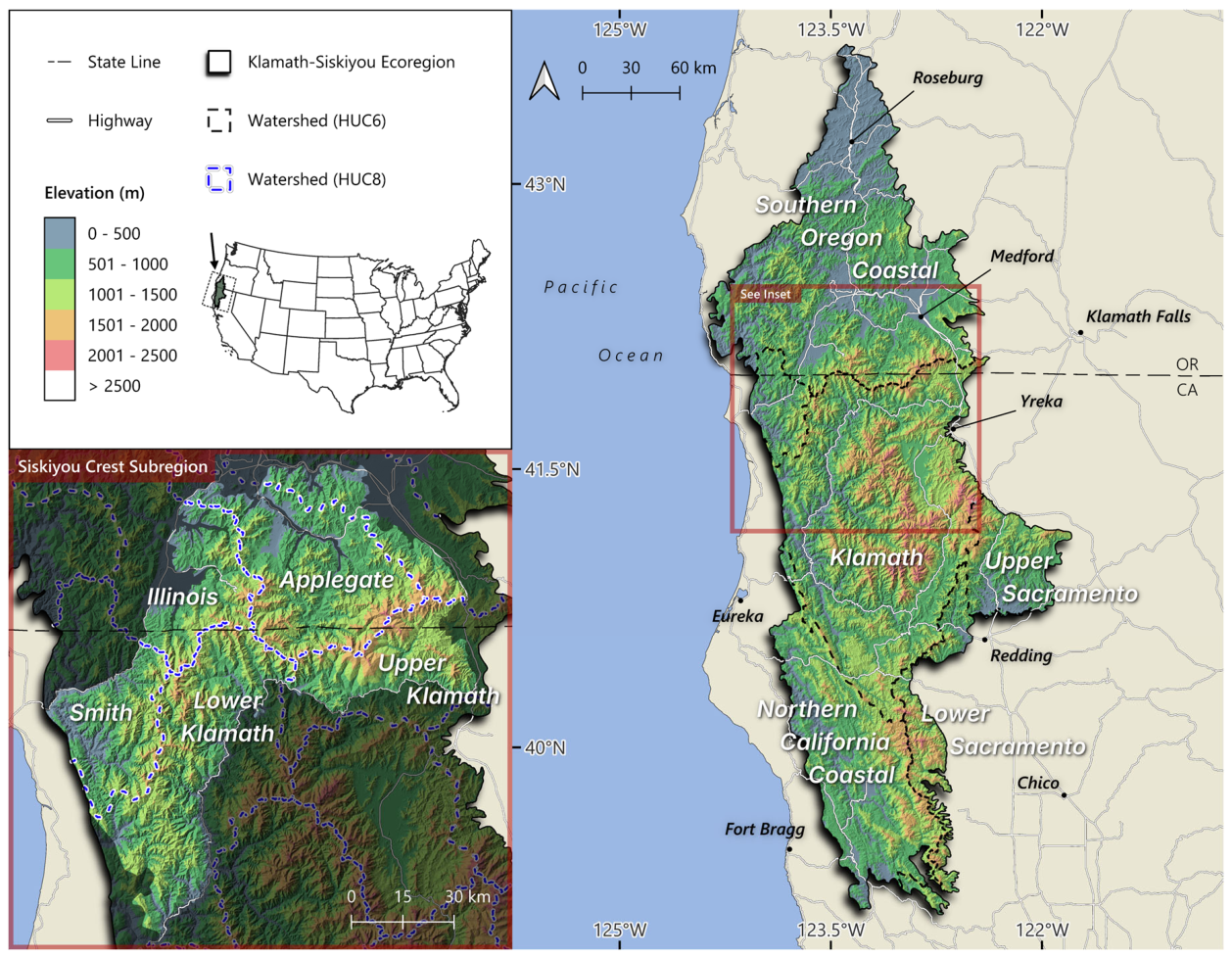
Figure 2.
The data collection and processing workflow for all analyses except those related to fuels and WUI as well as climate change.
Figure 2.
The data collection and processing workflow for all analyses except those related to fuels and WUI as well as climate change.
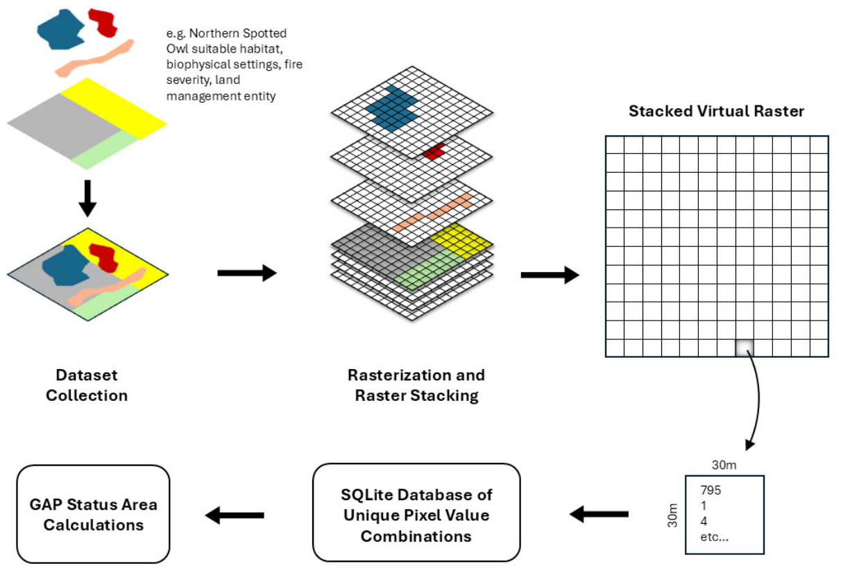
Figure 3.
Protection levels of elevation ranges within both the KSE and SCS with 30% and 50% protection targets for reference. Percentages are shown above the bars. Protected+ includes IRAs and select LWCs (managed “to protect”) that have been recognized for conservation importance but not fully protected.
Figure 3.
Protection levels of elevation ranges within both the KSE and SCS with 30% and 50% protection targets for reference. Percentages are shown above the bars. Protected+ includes IRAs and select LWCs (managed “to protect”) that have been recognized for conservation importance but not fully protected.
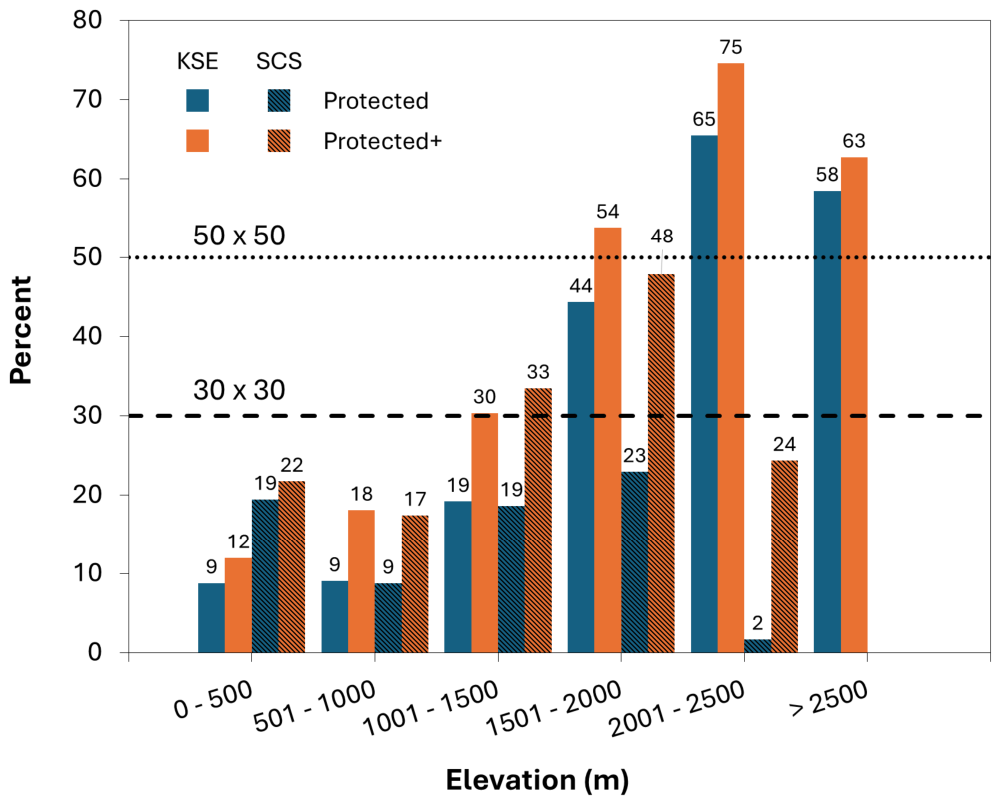
Figure 4.
GAP status of OGSI 80 and 200 in the KSE and SCS, showing high concentrations of mature and old-growth forest on lands with varying levels of protection in the SCS. Data from {Citation}.
Figure 4.
GAP status of OGSI 80 and 200 in the KSE and SCS, showing high concentrations of mature and old-growth forest on lands with varying levels of protection in the SCS. Data from {Citation}.
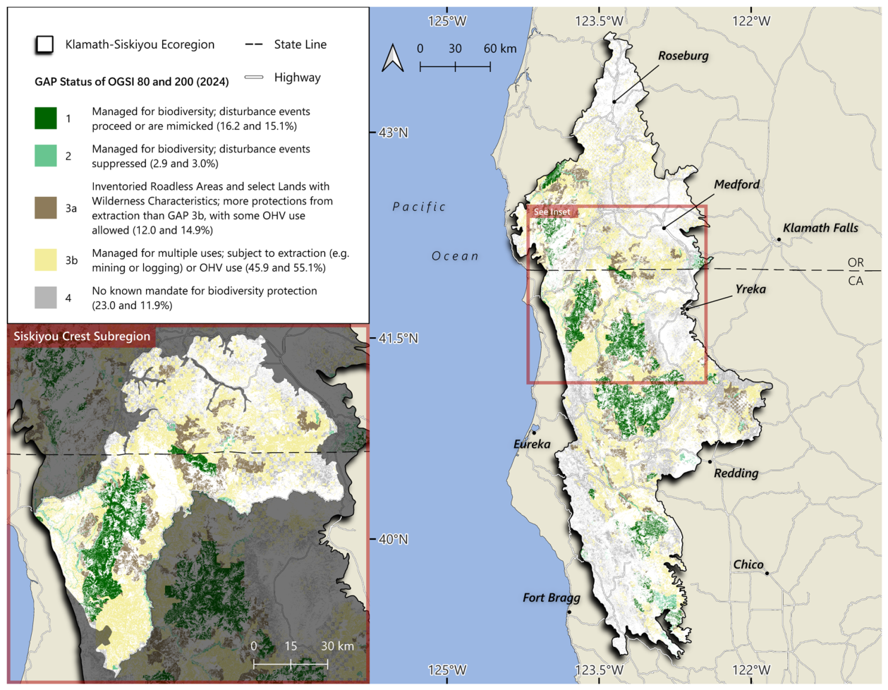
Figure 5.
GAP status of Pacific fisher connectivity conservation priority areas for the KSE and SCS.
Figure 5.
GAP status of Pacific fisher connectivity conservation priority areas for the KSE and SCS.
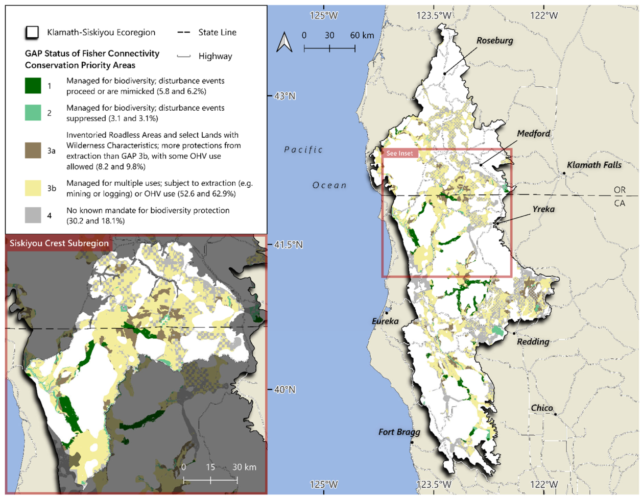
Figure 6.
Two large fires in the KSE and SCS in 2020 in relation to GAP status and fire severity levels. Note the high concentrations of high severity fire within GAP status 3b.
Figure 6.
Two large fires in the KSE and SCS in 2020 in relation to GAP status and fire severity levels. Note the high concentrations of high severity fire within GAP status 3b.
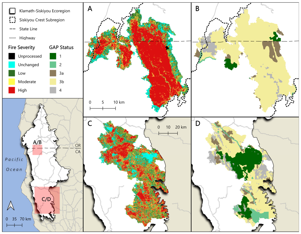
Figure 7.
Fuel treatments in relation to WUI areas and whether federal land management agencies classified the treatment as occurring within WUI.
Figure 7.
Fuel treatments in relation to WUI areas and whether federal land management agencies classified the treatment as occurring within WUI.
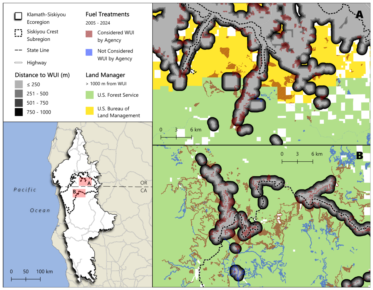
Figure 8.
Fuel treatments (hectares treated at least once) by federal agencies (BLM: Bureau of Land Management, USFS: USDA Forest Service) in relation to distance from the WUI for the KSE and SCS.
Figure 8.
Fuel treatments (hectares treated at least once) by federal agencies (BLM: Bureau of Land Management, USFS: USDA Forest Service) in relation to distance from the WUI for the KSE and SCS.
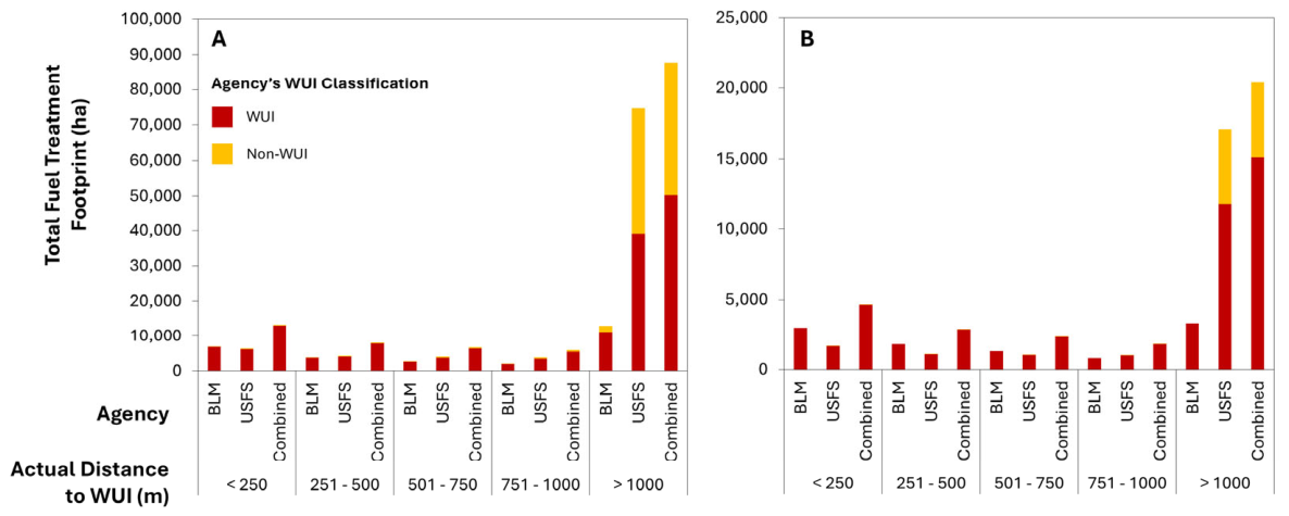
Figure 9.
Model median growing-degree days for the historical period (1950-2010) and the model median projected change for the 2010-2039, 2040-2069, and 2070-2099 periods relative to historical values under the intermediate (SSP245) and very high (SSP585) emission scenario for the KSE and SCS (outline in black, also see Figure S8 for a zoom in on the SCS). Growing degree-days is defined as the total number of annual degree-days >10°C and is an indicator of heat accumulation and heat availability for plant growth.
Figure 9.
Model median growing-degree days for the historical period (1950-2010) and the model median projected change for the 2010-2039, 2040-2069, and 2070-2099 periods relative to historical values under the intermediate (SSP245) and very high (SSP585) emission scenario for the KSE and SCS (outline in black, also see Figure S8 for a zoom in on the SCS). Growing degree-days is defined as the total number of annual degree-days >10°C and is an indicator of heat accumulation and heat availability for plant growth.
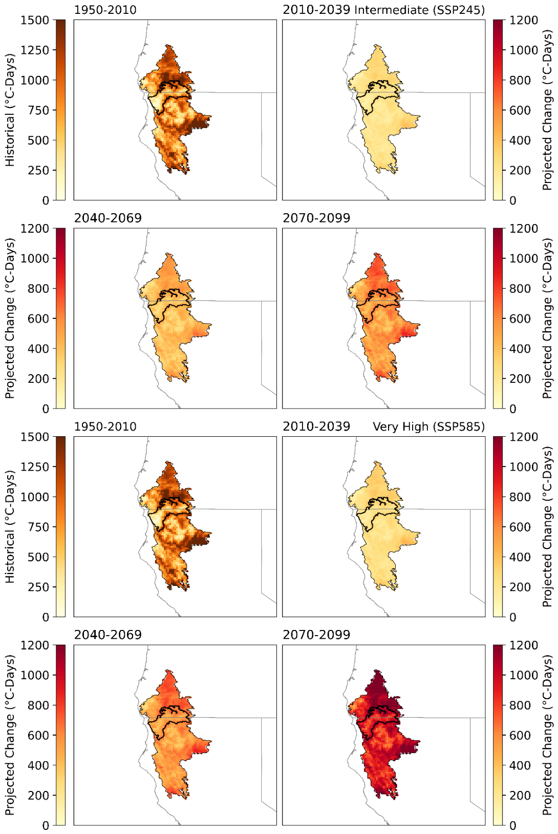
Figure 10.
Model mean historical (1950-201) mean summer (JJA) maximum temperature and model mean summer temperature for the periods 2010-2039, 2040-2069, and 2070-2099 relative to the historical period under the intermediate (SSP245) and very high (SSP585) emissions scenarios for the KSE and SCS (black outline, also see Figure S9 for a zoom in on the SCS).
Figure 10.
Model mean historical (1950-201) mean summer (JJA) maximum temperature and model mean summer temperature for the periods 2010-2039, 2040-2069, and 2070-2099 relative to the historical period under the intermediate (SSP245) and very high (SSP585) emissions scenarios for the KSE and SCS (black outline, also see Figure S9 for a zoom in on the SCS).
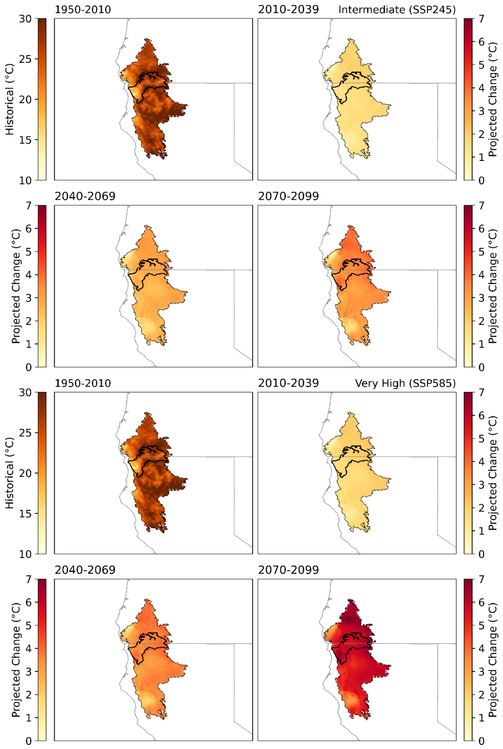
Figure 11.
Model median historical (1950-2010) total summer (JJA) precipitation and model median projected change in total summer precipitation for the time periods 2010-2039, 2040-2069, and 2070-2099 relative to the historical period under the intermediate (SSP245) and very high (SSP585) emissions scenario for the KSE and SCS (black outline, also see Figure S10 for a zoom in on the SCS).
Figure 11.
Model median historical (1950-2010) total summer (JJA) precipitation and model median projected change in total summer precipitation for the time periods 2010-2039, 2040-2069, and 2070-2099 relative to the historical period under the intermediate (SSP245) and very high (SSP585) emissions scenario for the KSE and SCS (black outline, also see Figure S10 for a zoom in on the SCS).
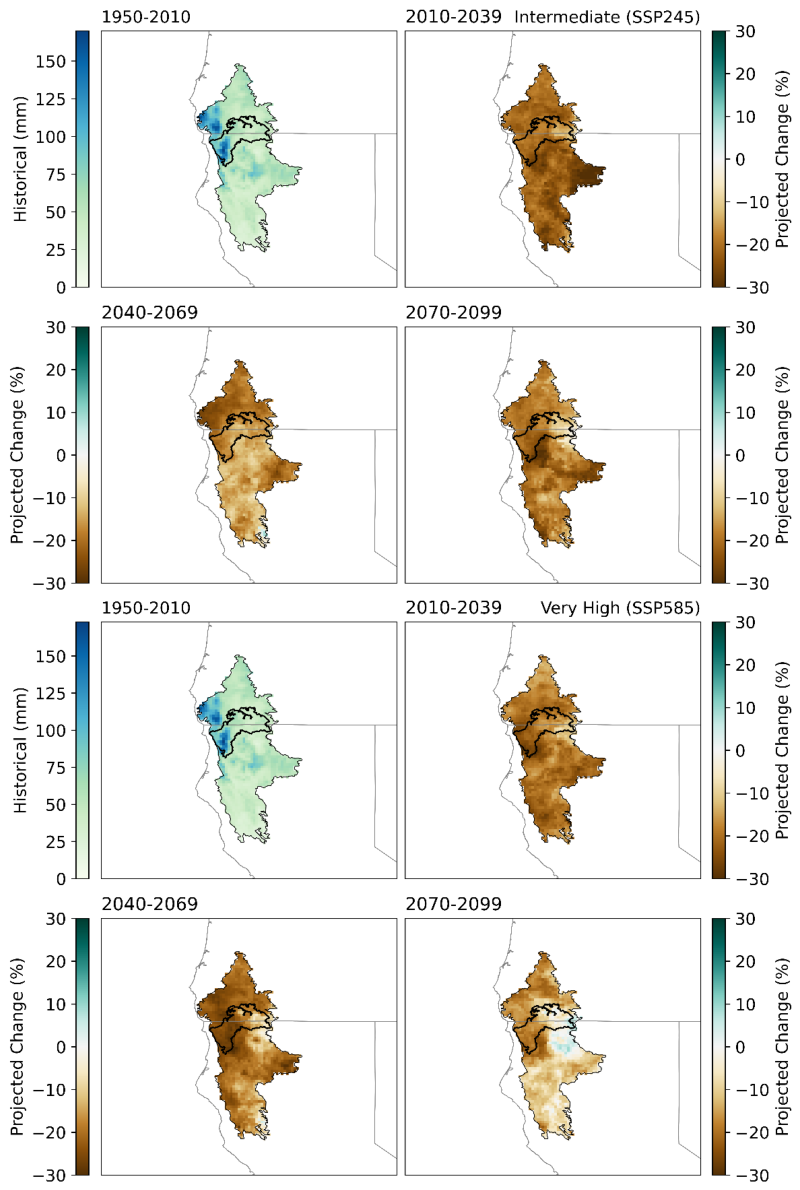
Figure 12.
Model median April 1st snow-water equivalent (SWE) for the historical period (1950-2010) and the model median projected percent change in April 1st SWE relative to the historical period for the 2020-2049, 2040-2069, and 2070-2099 periods under the intermediate (RCP 4.5) and very high (RCP 8.5) climate scenarios for the KSE and the SCS (outlined in black, also see Figure S11 for a zoom in on the SCS). Grid cells with <10-mm of April 1st SWE are treated as having no historical April 1st SWE.
Figure 12.
Model median April 1st snow-water equivalent (SWE) for the historical period (1950-2010) and the model median projected percent change in April 1st SWE relative to the historical period for the 2020-2049, 2040-2069, and 2070-2099 periods under the intermediate (RCP 4.5) and very high (RCP 8.5) climate scenarios for the KSE and the SCS (outlined in black, also see Figure S11 for a zoom in on the SCS). Grid cells with <10-mm of April 1st SWE are treated as having no historical April 1st SWE.
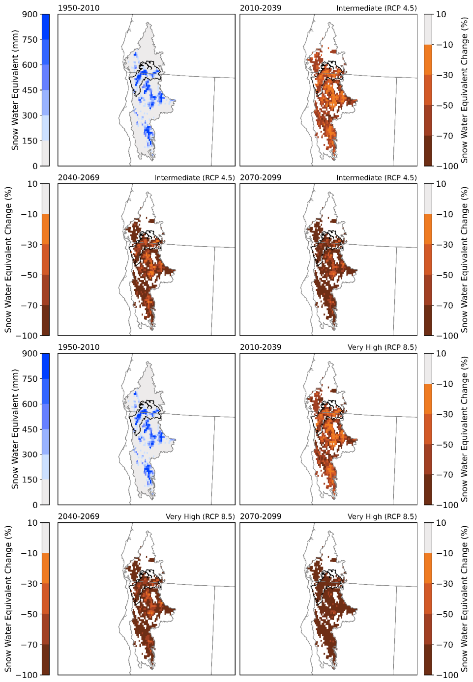
Figure 13.
The average historical (1950-2010) and future likelihood of climate and fuel condition conducive for wildfire for the 2020-2049, 2040-2069, and 2070-2099 periods under both the intermediate (RCP 4.5) and very high (RCP 8.5) climate change scenarios for the KSE and SCS (black outline, also see Figure S12 for a zoom in on the SCS). These projections assume that fire suppression efforts are implemented in the future. We define the wildlife likelihood as the proportion of years within each range of years with climate and fuel (vegetation) conditions conducive for wildfire.
Figure 13.
The average historical (1950-2010) and future likelihood of climate and fuel condition conducive for wildfire for the 2020-2049, 2040-2069, and 2070-2099 periods under both the intermediate (RCP 4.5) and very high (RCP 8.5) climate change scenarios for the KSE and SCS (black outline, also see Figure S12 for a zoom in on the SCS). These projections assume that fire suppression efforts are implemented in the future. We define the wildlife likelihood as the proportion of years within each range of years with climate and fuel (vegetation) conditions conducive for wildfire.
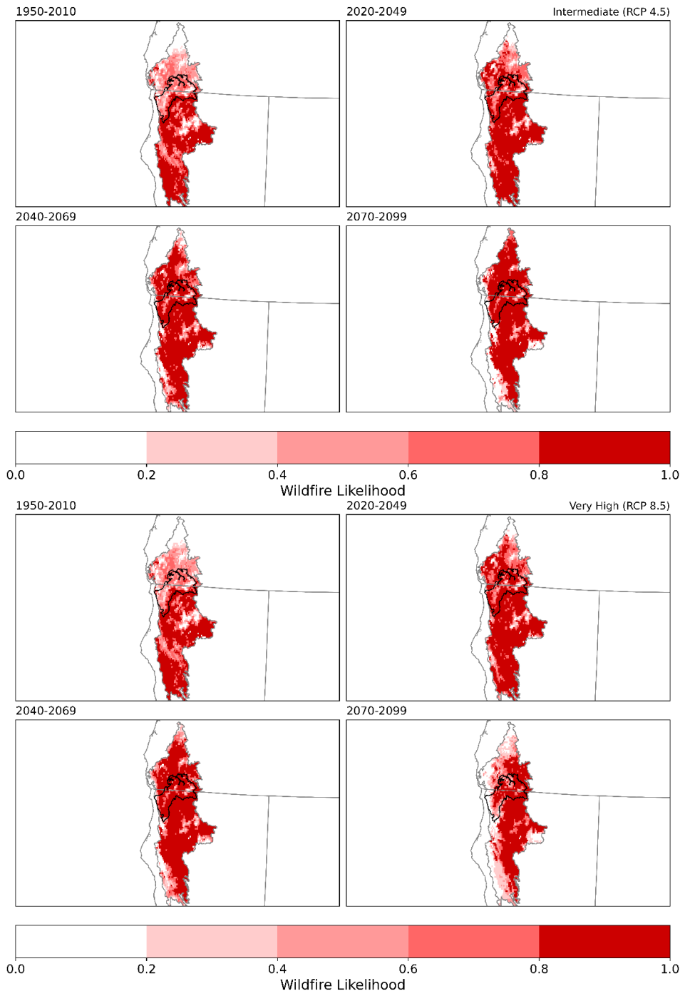

Table 1.
Landownerships and US Geological Survey Gap Analysis Program (GAP) categories for the KSE and SCS. IRAs and select LWCs (managed “to protect”) are GAP 3a. “Other” includes lands owned or managed by local jurisdictions (e.g., city or county) and non-governmental organizations.
Table 1.
Landownerships and US Geological Survey Gap Analysis Program (GAP) categories for the KSE and SCS. IRAs and select LWCs (managed “to protect”) are GAP 3a. “Other” includes lands owned or managed by local jurisdictions (e.g., city or county) and non-governmental organizations.
| Klamath-Siskiyou Ecoregion | ||||||
|---|---|---|---|---|---|---|
| Land Management Entity | GAP ha | |||||
| (%) | Total ha | |||||
| 1 | 2 | 3a | 3b | 4 | (%) | |
| U.S. National Park Service | 417 | 17,219 | 271 | 7 | 908 | 18,822 |
| (2.2) | (91.5) | (1.4) | (0.0) | (4.8) | (0.4) | |
| USDA Forest Service | 601,364 | 108,472 | 412,844 | 1,280,587 | 0 | 2,403,267 |
| (25.0) | (4.5) | (17.2) | (53.3) | (0.0) | (49.7) | |
| U.S. Bureau of Land Management | 21,169 | 17,493 | 25,650 | 399,271 | 0 | 463,582 |
| (4.6) | (3.8) | (5.5) | (86.1) | (0.0) | (9.6) | |
| Tribal | 0 | 0 | 0 | 0 | 58,943 | 58,943 |
| (0.0) | (0.0) | (0.0) | (0.0) | (100.0) | (1.2) | |
| State | 524 | 2940 | 4 | 16,320 | 2109 | 21,897 |
| (2.4) | (13.4) | (0.0) | (74.5) | (9.6) | (0.5) | |
| Other | 619 | 5583 | 0 | 4441 | 3974 | 14,617 |
| (4.2) | (38.2) | (0.0) | (30.4) | (27.2) | (0.3) | |
| Private | 111 | 1309 | 1 | 2235 | 1,851,023 | 1,854,677 |
| (0.0) | (0.1) | (0.0) | (0.1) | (99.8) | (38.4) | |
| Total ha | 624,204 | 153,016 | 438,769 | 1,702,860 | 1,916,957 | 4,835,805 |
| % | (12.9) | (3.2) | (9.1) | (35.2) | (39.6) | (100.0) |
| Siskiyou Crest Subregion | ||||||
| U.S. National Park Service | 406 | 647 | 271 | 7 | 907 | 2237 |
| (18.1) | (28.9) | (12.1) | (0.3) | (40.5) | (0.3) | |
| USDA Forest Service | 80,885 | 19,572 | 78,210 | 278,706 | 0 | 457,373 |
| (17.7) | (4.3) | (17.1) | (60.9) | (0.0) | (65.5) | |
| U.S. Bureau of Land Management | 0 | 186 | 4536 | 84,746 | 0 | 89,469 |
| (0.0) | (0.2) | (5.1) | (94.7) | (0.0) | (12.8) | |
| Tribal | 0 | 0 | 0 | 0 | 123 | 123 |
| (0.0) | (0.0) | (0.0) | (0.0) | (100.0) | (0.0) | |
| State | 0 | 37 | 0 | 1491 | 322 | 1850 |
| (0.0) | (2.0) | (0.0) | (80.6) | (17.4) | (0.3) | |
| Other | 0 | 42 | 0 | 436 | 40 | 517 |
| (0.0) | (8.1) | (0.0) | (84.3) | (7.7) | (0.1) | |
| Private | 0 | 143 | 0 | 693 | 146,351 | 147,187 |
| (0.0) | (0.1) | (0.0) | (0.5) | (99.4) | (21.1) | |
| Total ha | 81,291 | 20,626 | 83,017 | 366,079 | 147,742 | 698,755 |
| % | (11.6) | (3.0) | (11.9) | (52.4) | (21.1) | (100.0) |
Table 2.
Modified BPS subgroups for the KSE and SCS. Green color indicates a conservation target was met in GAP 1 and 2 coverages. Blue color indicates the added contribution to meeting protection targets if GAP 3a is included with GAP 1 and 2.
Table 2.
Modified BPS subgroups for the KSE and SCS. Green color indicates a conservation target was met in GAP 1 and 2 coverages. Blue color indicates the added contribution to meeting protection targets if GAP 3a is included with GAP 1 and 2.
| Klamath-Siskiyou Ecoregion | ||||||
|---|---|---|---|---|---|---|
| Modified BPS (Group) | GAP ha | |||||
| (%) | Total ha | |||||
| 1 | 2 | 3a | 3b | 4 | (%) | |
| Agricultural | 147 | 931 | 15 | 1406 | 137,265 | 139,764 |
| (0.1) | (0.7) | (0.0) | (1.0) | (98.2) | (2.9) | |
| Barren and Sparsely Vegetated | 3137 | 646 | 750 | 3635 | 4316 | 12,486 |
| (25.1) | (5.2) | (6.0) | (29.1) | (34.6) | (0.3) | |
| Blue Oak-Foothill Pine Woodland and Savanna | 1264 | 4922 | 1889 | 7715 | 41,474 | 57,264 |
| (2.2) | (8.6) | (3.3) | (13.5) | (72.4) | (1.2) | |
| California Mixed Evergreen Forest and Woodland | 100,945 | 29,121 | 109,457 | 330,734 | 247,774 | 818,031 |
| (12.3) | (3.6) | (13.4) | (40.4) | (30.3) | (16.9) | |
| Chaparral | 46,633 | 8150 | 11,473 | 36,481 | 60,933 | 163,671 |
| (28.5) | (5.0) | (7.0) | (22.3) | (37.2) | (3.4) | |
| Developed | 8849 | 7035 | 4253 | 93,184 | 141,865 | 255,186 |
| (3.5) | (2.8) | (1.7) | (36.5) | (55.6) | (5.3) | |
| Dry Douglas-fir Forest and Woodland | 27 | 277 | 753 | 6578 | 10,225 | 17,860 |
| (0.2) | (1.6) | (4.2) | (36.8) | (57.3) | (0.4) | |
| Dry Mixed Conifer Forest and Woodland | 138,566 | 50,137 | 150,153 | 586,799 | 578,633 | 1,504,287 |
| (9.2) | (3.3) | (10.0) | (39.0) | (38.5) | (31.1) | |
| Grassland | 1314 | 1370 | 1308 | 4491 | 29,053 | 37,535 |
| (3.5) | (3.7) | (3.5) | (12.0) | (77.4) | (0.8) | |
| Juniper Woodland and Savanna | 455 | 68 | 41 | 569 | 2766 | 3900 |
| (11.7) | (1.8) | (1.1) | (14.6) | (70.9) | (0.1) | |
| Mesic Mixed Conifer Forest and Woodland | 206,416 | 18,240 | 95,800 | 336,187 | 176,468 | 833,111 |
| (24.8) | (2.2) | (11.5) | (40.4) | (21.2) | (17.2) | |
| Oak Woodland and Savanna | 5046 | 4718 | 7014 | 25,773 | 64,167 | 106,718 |
| (4.7) | (4.4) | (6.6) | (24.2) | (60.1) | (2.2) | |
| Open Water | 1095 | 4289 | 163 | 19,693 | 11,443 | 36,682 |
| (3.0) | (11.7) | (0.4) | (53.7) | (31.2) | (0.8) | |
| Other Conifer Forest and Woodland | 60 | 84 | 84 | 961 | 476 | 1665 |
| (3.6) | (5.0) | (5.0) | (57.7) | (28.6) | (0.0) | |
| Other Hardwood Forest and Woodland | 220 | 36 | 126 | 643 | 713 | 1737 |
| (12.7) | (2.1) | (7.3) | (37.0) | (41.0) | (0.0) | |
| Other Shrubland | 2 | 1 | 1 | 58 | 915 | 976 |
| (0.2) | (0.1) | (0.1) | (5.9) | (93.8) | (0.0) | |
| Pacific Northwest Coastal Rainforest | 849 | 2828 | 1508 | 37,295 | 131,097 | 173,578 |
| (0.5) | (1.6) | (0.9) | (21.5) | (75.5) | (3.6) | |
| Perennial Ice/Snow | 1720 | 0 | 0 | 7 | 9 | 1736 |
| (99.1) | (0.0) | (0.0) | (0.4) | (0.5) | (0.0) | |
| Ponderosa Pine Forest, Woodland and Savanna | 3669 | 9716 | 19,722 | 112,983 | 193,346 | 339,436 |
| (1.1) | (2.9) | (5.8) | (33.3) | (57.0) | (7.0) | |
| Red Fir Forest | 70,839 | 1155 | 17,541 | 33,879 | 9424 | 132,839 |
| (53.3) | (0.9) | (13.2) | (25.5) | (7.1) | (2.8) | |
| Riparian and Wetland | 23,475 | 9008 | 15,088 | 59,328 | 73,477 | 180,376 |
| (13.0) | (5.0) | (8.4) | (32.9) | (40.7) | (3.7) | |
| Subalpine Forest and Woodland | 9474 | 283 | 1630 | 4462 | 1117 | 16,966 |
| (55.8) | (1.7) | (9.6) | (26.3) | (6.6) | (0.4) | |
| Total ha | 624,204 | 153,016 | 438,769 | 1,702,860 | 1,916,957 | 4,835,805 |
| % | (12.9) | (3.2) | (9.1) | (35.2) | (39.6) | (100.0) |
| Siskiyou Crest Subregion | ||||||
| Agricultural | 1 | 24 | 12 | 61 | 5473 | 5571 |
| (0.0) | (0.4) | (0.2) | (1.1) | (98.2) | (0.8) | |
| Barren and Sparsely Vegetated | 73 | 75 | 37 | 114 | 73 | 371 |
| (19.6) | (20.3) | (10.0) | (30.6) | (19.5) | (0.1) | |
| Blue Oak-Foothill Pine Woodland and Savanna | 0 | 38 | 0 | 20 | 28 | 86 |
| (0.0) | (44.2) | (0.1) | (23.5) | (32.2) | (0.0) | |
| California Mixed Evergreen Forest and Woodland | 24,617 | 10,144 | 17,561 | 110,245 | 20,590 | 183,157 |
| (13.4) | (5.5) | (9.6) | (60.2) | (11.2) | (26.2) | |
| Chaparral | 5565 | 231 | 2078 | 3867 | 2210 | 13,951 |
| (39.9) | (1.7) | (14.9) | (27.7) | (15.8) | (2.0) | |
| Developed | 636 | 1032 | 466 | 23,269 | 13,005 | 38,408 |
| (1.7) | (2.7) | (1.2) | (60.6) | (33.9) | (5.5) | |
| Dry Douglas-fir Forest and Woodland | 0 | 14 | 72 | 2421 | 3913 | 6419 |
| (0.0) | (0.2) | (1.1) | (37.7) | (61.0) | (0.9) | |
| Dry Mixed Conifer Forest and Woodland | 35,931 | 4672 | 26,901 | 119,017 | 61,214 | 247,735 |
| (14.5) | (1.9) | (10.9) | (48.0) | (24.7) | (35.5) | |
| Grassland | 1 | 1 | 0 | 23 | 57 | 83 |
| (0.7) | (1.3) | (0.5) | (28.3) | (69.2) | (0.0) | |
| Juniper Woodland and Savanna | 0 | 0 | 0 | 34 | 53 | 87 |
| (0.0) | (0.0) | (0.0) | (39.1) | (60.9) | (0.0) | |
| Mesic Mixed Conifer Forest and Woodland | 6809 | 1192 | 21,619 | 56,548 | 16,055 | 102,224 |
| (6.7) | (1.2) | (21.2) | (55.3) | (15.7) | (14.6) | |
| Oak Woodland and Savanna | 1 | 27 | 10 | 1672 | 1294 | 3004 |
| (0.0) | (0.9) | (0.3) | (55.6) | (43.1) | (0.4) | |
| Open Water | 40 | 549 | 7 | 441 | 340 | 1377 |
| (2.9) | (39.9) | (0.5) | (32.0) | (24.7) | (0.2) | |
| Other Conifer Forest and Woodland | 0 | 16 | 0 | 3 | 45 | 64 |
| (0.0) | (25.0) | (0.0) | (4.3) | (70.6) | (0.0) | |
| Other Hardwood Forest and Woodland | 0 | 0 | 0 | 2 | 3 | 4 |
| (0.0) | (0.0) | (0.0) | (37.5) | (62.5) | (0.0) | |
| Other Shrubland | 0 | 0 | 0 | 0 | 0 | 0 |
| (0.0) | (0.0) | (0.0) | (100.0) | (0.0) | (0.0) | |
| Pacific Northwest Coastal Rainforest | 114 | 109 | 469 | 3023 | 898 | 4613 |
| (2.5) | (2.4) | (10.2) | (65.5) | (19.5) | (0.7) | |
| Ponderosa Pine Forest, Woodland and Savanna | 95 | 537 | 2852 | 24,185 | 17,080 | 44,749 |
| (0.2) | (1.2) | (6.4) | (54.0) | (38.2) | (6.4) | |
| Red Fir Forest | 3593 | 55 | 8354 | 11,504 | 1922 | 25,426 |
| (14.1) | (0.2) | (32.9) | (45.2) | (7.6) | (3.6) | |
| Riparian and Wetland | 3644 | 1908 | 2358 | 9271 | 3423 | 20,604 |
| (17.7) | (9.3) | (11.5) | (45.0) | (16.6) | (3.0) | |
| Subalpine Forest and Woodland | 172 | 0 | 220 | 362 | 67 | 821 |
| (20.9) | (0.0) | (26.8) | (44.1) | (8.1) | (0.1) | |
| Total ha | 81,291 | 20,626 | 83,017 | 366,079 | 147,742 | 698,755 |
| % | (11.6) | (3.0) | (11.9) | (52.4) | (21.1) | (100.0) |
Table 3.
Old Growth Structural Index 80 and 200 Persistence for the KSE and SCS, 1986-2024. Structural indices are based on USDA Forest Service mapping (Northwest Forest Plan Monitoring 2025) and persistence is based on areas that missed fires during this period.
Table 3.
Old Growth Structural Index 80 and 200 Persistence for the KSE and SCS, 1986-2024. Structural indices are based on USDA Forest Service mapping (Northwest Forest Plan Monitoring 2025) and persistence is based on areas that missed fires during this period.
| Klamath-Siskiyou Ecoregion | ||||||
|---|---|---|---|---|---|---|
| Old Growth Structure Index 200 (USDA Forest Service, 2025) | GAP ha | Total ha | ||||
| (%) | ||||||
| 1 | 2 | 3a | 3b | 4 | ||
| OGSI 80 | 284,335 | 54527 | 209,308 | 823,534 | 480,542 | 1,852,246 |
| (15.4) | (2.9) | (11.3) | (44.5) | (25.9) | ||
| OGSI 80 Persistence | 181,351 | 22756 | 110,705 | 252,564 | 35,640 | 603,016 |
| (30.1) | (3.8) | (18.4) | (41.9) | (5.9) | ||
| OGSI 80 Promotion to 200 | 111,048 | 13414 | 68,857 | 156,032 | 14,780 | 364,131 |
| (30.5) | (3.7) | (18.9) | (42.9) | (4.1) | ||
| OGSI 200 | 160,824 | 26223 | 121,645 | 436,594 | 150,365 | 895,651 |
| (18.0) | (2.9) | (13.6) | (48.8) | (16.8) | ||
| OGSI 200 Persistence | 90,032 | 11195 | 55,662 | 129,504 | 10,575 | 296,969 |
| (30.3) | (3.8) | (18.7) | (43.6) | (3.6) | ||
| Siskiyou Crest Subregion | ||||||
| OGSI 80 | 50,702 | 10693 | 48,501 | 191,597 | 46,613 | 348,105 |
| (14.6) | (3.1) | (13.9) | (55.0) | (13.4) | ||
| OGSI 80 Persistence | 33,419 | 1987 | 21,270 | 41,841 | 2,365 | 100,882 |
| (33.1) | (2.0) | (21.1) | (41.5) | (2.3) | ||
| OGSI 80 Promotion to 200 | 21,649 | 1171 | 14,458 | 26,973 | 1,160 | 65,411 |
| (33.1) | (1.8) | (22.1) | (41.2) | (1.8) | ||
| OGSI 200 | 31,390 | 5490 | 32,534 | 107,857 | 17,902 | 195,173 |
| (16.1) | (2.8) | (16.7) | (55.3) | (9.2) | ||
| OGSI 200 Persistence | 18,269 | 980 | 12,628 | 22,818 | 764 | 55,459 |
| (32.9) | (1.8) | (22.8) | (41.1) | (1.4) | ||
Table 4.
GAP status distribution across NSO current suitable and highly suitable habitat (2024) and suitable and highly suitable habitat that persisted from 1986 to 2024 despite burning at least once (persistence) for the KSE and SCS. Protected+ (GAP 3a) consists of IRAs and select LWCs.
Table 4.
GAP status distribution across NSO current suitable and highly suitable habitat (2024) and suitable and highly suitable habitat that persisted from 1986 to 2024 despite burning at least once (persistence) for the KSE and SCS. Protected+ (GAP 3a) consists of IRAs and select LWCs.
| Klamath-Siskiyou Ecoregion | ||||||
|---|---|---|---|---|---|---|
| Northern Spotted Owl Habitat (USDA Forest Service, 2025) | GAP ha | Total ha | ||||
| (%) | ||||||
| 1 | 2 | 3a | 3b | 4 | ||
| NSO Suitable/Highly Suitable (Combined) Habitat (2024) | 132,215 | 35,342 | 136,286 | 617,113 | 310,018 | 1,230,974 |
| (10.7) | (2.9) | (11.1) | (50.1) | (25.2) | ||
| Suitable | 57,247 | 13,437 | 47,674 | 215,831 | 153,309 | 487,498 |
| (11.7) | (2.8) | (9.8) | (44.3) | (31.5) | ||
| Highly Suitable | 74,968 | 21,905 | 88,612 | 401,282 | 156,710 | 743,476 |
| (10.1) | (3.0) | (11.9) | (54.0) | (21.1) | ||
| NSO Suitable/Highly Suitable Habitat Persistence | 77,441 | 11,690 | 63,581 | 142,813 | 12,684 | 308,208 |
| (25.1) | (3.8) | (20.6) | (46.3) | (4.1) | ||
| Suitable | 29,694 | 4003 | 20,489 | 44,669 | 5257 | 104,112 |
| (28.5) | (3.9) | (19.7) | (42.9) | (5.1) | ||
| Highly Suitable | 47,747 | 7686 | 43,092 | 98,144 | 7427 | 204,096 |
| (23.4) | (3.8) | (21.1) | (48.1) | (3.6) | ||
| Siskiyou Crest Subregion | ||||||
| NSO Suitable/Highly Suitable (Combined) Habitat (2024) | 32,259 | 11,486 | 31,627 | 176,107 | 40,028 | 291,507 |
| (11.1) | (3.9) | (10.9) | (60.4) | (13.7) | ||
| Suitable | 16,004 | 3767 | 12,750 | 61,728 | 19,355 | 113,603 |
| (14.1) | (3.3) | (11.2) | (54.3) | (17.0) | ||
| Highly Suitable | 16,255 | 7720 | 18,878 | 114,379 | 20,673 | 177,904 |
| (9.1) | (4.3) | (10.6) | (64.3) | (11.6) | ||
| NSO Suitable/Highly Suitable Habitat Persistence | 17,687 | 1798 | 12,523 | 27,315 | 1055 | 60,378 |
| (29.3) | (3.0) | (20.7) | (45.2) | (1.8) | ||
| Suitable | 8123 | 459 | 4375 | 8983 | 510 | 22,449 |
| (36.2) | (2.0) | (19.5) | (40.0) | (2.3) | ||
| Highly Suitable | 9564 | 1339 | 8148 | 18,332 | 545 | 37,929 |
| (25.2) | (3.5) | (21.5) | (48.3) | (1.4) | ||
Table 5.
Fire severity (1985-2023) across all land cover categories for the KSE and SCS in relation to GAP categories. 1 The percentages of each fire severity class for each GAP status are the percentage of a particular GAP status that experienced a particular fire severity (the sum of percentages for each GAP status column will equal 100%). 2 The percentages in the last column are the percentage of the total fire footprint in each severity class, irrespective of GAP status. 3 The percentages in the last row for the ecoregion and subregion represent the percentage of the total fire footprint across the study period that was in a particular GAP status.
Table 5.
Fire severity (1985-2023) across all land cover categories for the KSE and SCS in relation to GAP categories. 1 The percentages of each fire severity class for each GAP status are the percentage of a particular GAP status that experienced a particular fire severity (the sum of percentages for each GAP status column will equal 100%). 2 The percentages in the last column are the percentage of the total fire footprint in each severity class, irrespective of GAP status. 3 The percentages in the last row for the ecoregion and subregion represent the percentage of the total fire footprint across the study period that was in a particular GAP status.
| Klamath-Siskiyou Ecoregion | ||||||
|---|---|---|---|---|---|---|
| Fire Severity | GAP ha | Total ha (%) 2 |
||||
| (%) 1 | ||||||
| 1 | 2 | 3a | 3b | 4 | ||
| Unprocessed | 1111 | 1540 | 1045 | 530 | 315 | 4541 |
| (0.2) | (1.5) | (0.3) | (0.1) | (0.1) | (0.2) | |
| Unchanged | 41,330 | 7188 | 20,555 | 62,254 | 30,599 | 161,925 |
| (8.3) | (7.1) | (6.3) | (7.7) | (10.3) | (8.0) | |
| Low | 142,740 | 25,006 | 87,761 | 230,354 | 69,727 | 555,587 |
| (28.6) | (24.8) | (26.9) | (28.4) | (23.4) | (27.3) | |
| Moderate | 137,790 | 26,728 | 93,729 | 215,764 | 84,758 | 558,769 |
| (27.6) | (26.6) | (28.7) | (26.6) | (28.4) | (27.5) | |
| High | 176,156 | 40,201 | 123,244 | 300,958 | 112,756 | 753,314 |
| (35.3) | (39.9) | (37.8) | (37.2) | (37.8) | (37.0) | |
| Total ha | 499,127 | 100,661 | 326,333 | 809,860 | 298,154 | 2,034,136 |
| (%) 3 | (24.5) | (4.9) | (16.0) | (39.8) | (14.7) | |
| Siskiyou Crest Subregion | ||||||
| Unprocessed | 56 | 10 | 854 | 145 | 41 | 1106 |
| (0.1) | (0.2) | (1.7) | (0.1) | (0.2) | (0.4) | |
| Unchanged | 8148 | 1040 | 3507 | 11,616 | 2416 | 26,726 |
| (13.0) | (16.9) | (7.0) | (9.2) | (10.9) | (10.0) | |
| Low | 21,155 | 2495 | 15,056 | 34,556 | 4808 | 78,071 |
| (33.8) | (40.5) | (29.9) | (27.3) | (21.8) | (29.2) | |
| Moderate | 16,008 | 1401 | 14,424 | 27,353 | 5769 | 64,955 |
| (25.6) | (22.7) | (28.6) | (21.6) | (26.1) | (24.3) | |
| High | 17,170 | 1214 | 16,524 | 52,889 | 9067 | 96,865 |
| (27.5) | (19.7) | (32.8) | (41.8) | (41.0) | (36.2) | |
| Total ha | 62,538 | 6159 | 50,365 | 126,559 | 22,101 | 267,722 |
| (%) 3 | (23.4) | (2.3) | (18.8) | (47.3) | (8.3) | |
Table 6.
Fire severity (1985-2023) across dry and mesic mixed conifer forest and woodland, dry Douglas-fir forest and woodland, and ponderosa pine forest, woodland and savanna land cover categories for the KSE and SCS in relation to GAP categories. 1 The percentages of each fire severity class for each GAP status are the percentage of a particular GAP status that experienced a particular fire severity (the sum of percentages for each GAP status column will equal 100%). 2 The percentages in the last column are the percentage of the total fire footprint in each severity class, irrespective of GAP status. 3 The percentages in the last row for the ecoregion and subregion represent the percentage of the total fire footprint across the study period that was in a particular GAP status.
Table 6.
Fire severity (1985-2023) across dry and mesic mixed conifer forest and woodland, dry Douglas-fir forest and woodland, and ponderosa pine forest, woodland and savanna land cover categories for the KSE and SCS in relation to GAP categories. 1 The percentages of each fire severity class for each GAP status are the percentage of a particular GAP status that experienced a particular fire severity (the sum of percentages for each GAP status column will equal 100%). 2 The percentages in the last column are the percentage of the total fire footprint in each severity class, irrespective of GAP status. 3 The percentages in the last row for the ecoregion and subregion represent the percentage of the total fire footprint across the study period that was in a particular GAP status.
| Klamath-Siskiyou Ecoregion | ||||||
|---|---|---|---|---|---|---|
| Fire Severity | GAP ha | Total ha (%) 2 |
||||
| (%) 1 | ||||||
| 1 | 2 | 3a | 3b | 4 | ||
| Unprocessed | 401 | 54 | 171 | 266 | 159 | 1051 |
| (0.1) | (0.1) | (0.1) | (0.0) | (0.1) | (0.1) | |
| Unchanged | 20,752 | 3264 | 12,539 | 36,136 | 16,555 | 89,245 |
| (6.9) | (5.6) | (6.0) | (6.7) | (8.4) | (6.8) | |
| Low | 84,342 | 14,934 | 52,887 | 148,118 | 44,693 | 344,974 |
| (28.1) | (25.8) | (25.4) | (27.3) | (22.6) | (26.4) | |
| Moderate | 87,472 | 15,792 | 61,317 | 149,053 | 58,105 | 371,740 |
| (29.1) | (27.3) | (29.4) | (27.5) | (29.3) | (28.4) | |
| High | 107,353 | 23,881 | 81,480 | 208,685 | 78,513 | 499,911 |
| (35.7) | (41.2) | (39.1) | (38.5) | (39.6) | (38.3) | |
| Total ha | 300,320 | 57,924 | 208,393 | 542,258 | 198,025 | 1,306,921 |
| (%) 3 | (23.0) | (4.4) | (15.9) | (41.5) | (15.2) | |
| Siskiyou Crest Subregion | ||||||
| Unprocessed | 17 | 2 | 85 | 57 | 4 | 1106 |
| (0.1) | (0.1) | (0.3) | (0.1) | (0.0) | (0.7) | |
| Unchanged | 3447 | 186 | 2398 | 5880 | 1694 | 26,726 |
| (10.3) | (10.2) | (7.4) | (8.4) | (10.2) | (17.3) | |
| Low | 9906 | 631 | 9385 | 17,680 | 3495 | 78,071 |
| (29.5) | (34.7) | (28.9) | (25.1) | (21.1) | (50.4) | |
| Moderate | 9483 | 447 | 9185 | 16,034 | 4553 | 64,955 |
| (28.2) | (24.5) | (28.3) | (22.8) | (27.5) | (42.0) | |
| High | 10,735 | 555 | 11,378 | 30,746 | 6812 | 96,865 |
| (32.0) | (30.5) | (35.1) | (43.7) | (41.1) | (62.6) | |
| Total ha | 33,590 | 1819 | 32,430 | 70,398 | 16,557 | 154,795 |
| (%) 3 | (21.7) | (1.2) | (21.0) | (45.5) | (10.7) | |
Table 7.
Ecoregional conservation assessments for the Klamath-Siskiyou/Siskiyou Crest (this study), Northern Rockies/Yaak Valley [6], Southern Rockies/Santa Fe [5], and Mogollon Highlands [4]. Note: the Mogollon Highlands did not include a specific subregional analysis.
| Location | Area (M ha) | % Protected |
|---|---|---|
| Klamath-Siskiyou Ecoregion | 4.83 | 15 |
| Siskiyou Crest Subregion of KSE | 0.68 | 14.5 |
| Northern Rockies Ecoregion (NRE) | 8.19 | 2.2 |
| Yaak Valley Subregion of NRE | 0.16 | 0.25 |
| Southern Rockies Ecoregion (SRE) | 14.5 | 18.4 |
| Sant Fe Watershed Subregion of SRE | 2.2 | 12.1 |
| Mogollon Highlands Ecoregion | 11.3 | 9 |
Table 8.
Results of fuel treatment distance to WUI analyses in ecoregional conservation assessments for the Klamath-Siskiyou/Siskiyou Crest (this study), Northern Rockies/Yaak Valley [6], and Southern Rockies/Santa Fe [5].
| Location | Fuel Treatment Distance to WUI (m) | ||||
| 0 - 250 | 251 - 500 | 501 - 750 | 751 - 1000 | >1000 | |
| Klamath-Siskiyou Ecoregion | 10.9 | 6.6 | 5.6 | 4.9 | 72.0 |
| Siskiyou Crest Subregion of KSE | 14.5 | 9.0 | 7.3 | 5.7 | 63.5 |
| Northern Rockies Ecoregion (NRE) | 5.7 | 4.1 | 3.9 | 3.7 | 82.6 |
| Yaak Valley Subregion of NRE | 8.5 | 10.1 | 8.6 | 7.4 | 65.5 |
| Southern Rockies Ecoregion (SRE) | 8.1 | 6.9 | 5.8 | 5.7 | 73.5 |
| Sant Fe Watershed Subregion of SRE | 4.4 | 5.2 | 4.9 | 5.7 | 79.7 |
Disclaimer/Publisher’s Note: The statements, opinions and data contained in all publications are solely those of the individual author(s) and contributor(s) and not of MDPI and/or the editor(s). MDPI and/or the editor(s) disclaim responsibility for any injury to people or property resulting from any ideas, methods, instructions or products referred to in the content. |
© 2026 by the authors. Licensee MDPI, Basel, Switzerland. This article is an open access article distributed under the terms and conditions of the Creative Commons Attribution (CC BY) license (http://creativecommons.org/licenses/by/4.0/).
Copyright: This open access article is published under a Creative Commons CC BY 4.0 license, which permit the free download, distribution, and reuse, provided that the author and preprint are cited in any reuse.


