Holographic-Inspired Dynamical Dark Energy with Running Dimension

1. Introduction

The standard cosmological model, $\Lambda$CDM, has achieved remarkable empirical success in describing a wide range of observations, from the cosmic microwave background (CMB) anisotropies [2]. to the large-scale structure of the universe [3] and the luminosity-distance relation of type Ia supernovae [4]. Nevertheless, several persistent tensions have emerged at the level of $3\sigma$ to $5\sigma$ significance, most notably the Hubble constant ($H_0$) tension between early-universe CMB inferences [5] and late-time direct measurements [6], and the growth tension ($S_8$) manifesting as a discrepancy between the amplitude of matter clustering predicted by $\Lambda$CDM and that inferred from weak lensing and redshift-space distortion surveys [7,8]. These tensions, while not yet conclusive, motivate serious consideration of extensions to the minimal dark energy sector, particularly those that allow for a dynamical equation of state $w\left(z\right)$ and a modification of the growth history while respecting the stringent constraints from CMB and baryon acoustic oscillations (BAO) [9].

A substantial fraction of phenomenological dark energy models introduce an ad hoc parametrization of $w\left(z\right)$, such as the Chevallier-Polarski-Linder (CPL) form, which, despite its flexibility, lacks a well-defined microscopic or holographic origin and does not naturally address the growth tension [10]. Moreover, purely phenomenological models often suffer from an under-determined parameter space when fitted to current data, leading to posterior distributions that are prior-dominated and difficult to interpret physically [11]. What remains missing is a unified approach that derives the redshift evolution of the dark energy equation of state from a first-principles-motivated framework—ideally one that couples an infrared (IR) cutoff inspired by holographic principles with a theoretically controlled ultraviolet (UV) completion scale—while simultaneously predicting a suppression of growth at low redshifts, thereby attacking both the $H_0$ and $S_8$ tensions with a minimal set of physically justified parameters.

In response to this gap, the present work introduces a dynamical dark energy model derived from a scalar-tensor action augmented by a conformal anomaly term originating from a TeV-scale sector, leading to a running effective dimension $\alpha \left(z\right)$ that directly modifies the holographic infrared cutoff. The model yields a closed-form $w\left(z\right)$ expression that retains only one free parameter (the transition redshift) after fixing the TeV scale by particle-physics considerations, and predicts a measurable decrease in ${\sigma }_8$ relative to $\Lambda$CDM without violating CMB constraints. This constitutes a value proposition: a theoretically conservative but observationally testable extension of $\Lambda$CDM that addresses both major tensions by altering the late-time expansion and growth histories in a mutually consistent way, using a framework that is falsifiable with upcoming Stage-IV dark energy surveys [12].

2. Formulation

2.1. Action Principle and Anomalous Coupling

We start from the following effective action in the Jordan frame, defined on a 4D spacetime manifold with metric signature $(-,+,+,+)$:

$$S=\int d^{4}x\sqrt{-g}\left[{\displaystyle \frac{M_{\mathrm{Pl}}^2}{2}}R-{\displaystyle \frac{1}{2}}{\partial }_{\mu }\varphi {\partial }^{\mu }\varphi -V\left(\varphi \right)+{\displaystyle \frac{\lambda \left(\varphi \right)}{16{\pi }^2}}{G}_{\mu \nu }^a{G}^{a\mu \nu }\right]+S_{\mathrm{m}}[g_{\mu \nu },{\psi }_{\mathrm{m}}],$$

(1)

where $M_{\mathrm{Pl}}={\left(8\pi G\right)}^{-1/2}$ is the reduced Planck mass, R is the Ricci scalar, $\varphi$ is a canonical scalar field (the dark energy candidate), $V\left(\varphi \right)$ is its potential, $G_{\mu \nu }^a$ is the field strength of a non-abelian gauge field (taken for definiteness to be an SU(3) hidden sector), and $\lambda \left(\varphi \right)$ is a dimensionless coupling function. The term proportional to $G_{\mu \nu }^a{G}^{a\mu \nu }$ is the trace anomaly, which arises from integrating out heavy fermions or from string-theoretic corrections; its coefficient is protected by non-renormalization theorems [13]. The matter action $S_{\mathrm{m}}$ describes baryons, cold dark matter, and radiation, minimally coupled to $g_{\mu \nu }$. We assume a flat Friedmann-Lemaître-Robertson-Walker (FLRW) metric:

$$d{s}^2=-d{t}^2+a{\left(t\right)}^2{\delta }_{ij}d{x}^{i}d{x}^j,a\left(t\right)={\displaystyle \frac{1}{1+z}}.$$

(2)

2.2. Holographic and the Running Dimension

The holographic principle posits that the number of degrees of freedom in a volume scales with its bounding surface area [14]. In the context of dark energy, this motivates an infrared cutoff L such that the dark energy density is ${\rho }_{\mathrm{DE}}\propto L^{-2}$ [15]. The simplest choice $L=H^{-1}$ leads to ${\rho }_{\mathrm{DE}}\propto H^2$, which tracks the critical density but yields an equation of state $w=-1$ exactly only for a constant H [15]. A generalization introduces a dimensionless parameter $\alpha$:

$$L_{\mathrm{eff}}={\displaystyle \frac{1}{H(1+\alpha )}}\Rightarrow {\rho }_{\mathrm{DE}}={\displaystyle \frac{3c^2{M}_{\mathrm{Pl}}^2{H}^2}{{(1+\alpha )}^2}},$$

(3)

where c is a constant of order unity. This form respects the covariant entropy bound [16] provided $\alpha \ge -1$; we will later find $\alpha \ge 0$ from stability. The key innovation of this work is to promote $\alpha$ to a function of redshift, $\alpha \left(z\right)$, thereby making the infrared cutoff dynamical. The physical origin of this running is the anomalous term in the action: the coupling $\lambda \left(\varphi \right)$ induces a scale-dependent shift in the effective dimension of the field theory, as seen in the spectral dimension of quantum gravity [17]. Translating the renormalization-group running from the UV cutoff ${\Lambda }_{\mathrm{UV}}\sim 13.6\mathrm{TeV}$ (the LHC scale) to the IR scale H yields, after integrating the one-loop beta function for the anomaly coefficient, the following expression:

$$\alpha \left(z\right)={\alpha }_0\left[1-tanh\left(\beta {\displaystyle \frac{z}{z_c}}\right)\right]+{\alpha }_{\mathrm{UV}}{\displaystyle \frac{{\Lambda }_{\mathrm{QCD}}^2}{M_{\mathrm{TeV}}^2}}{(1+z)}^3.$$

(4)

Here ${\alpha }_0\simeq 0.1$ is the present-day value, $\beta >0$ controls the sharpness of the transition, $z_c$ is the transition redshift where $\alpha$ drops significantly, ${\Lambda }_{\mathrm{QCD}}\sim 300\mathrm{MeV}$ is the QCD scale, $M_{\mathrm{TeV}}=13.6\mathrm{TeV}$ is the UV scale (chosen as the highest energy probed by the LHC, beyond which new physics may appear [18]), and ${\alpha }_{\mathrm{UV}}$ is a dimensionless coefficient fixed by matching to the anomaly calculation to be ${\alpha }_{\mathrm{UV}}=\mathcal{O}\left(1\right)$. The ${(1+z)}^3$ factor arises from the redshift scaling of the number density of heavy particles that contribute to the anomaly. The tanh term captures a smooth crossover from an early-universe phase where $\alpha$ is larger (implying stronger deviation from 4D) to the late universe where $\alpha$ tends to ${\alpha }_0$. This form is chosen because it satisfies: (i) $\alpha (z\to \infty )\to {\alpha }_0(1-1)+{\alpha }_{\mathrm{UV}}\times \mathrm{small}\approx 0$, reverting to $\Lambda$CDM at high redshift; (ii) $\alpha (z=0)={\alpha }_0+{\alpha }_{\mathrm{UV}}{({\Lambda }_{\mathrm{QCD}}/M_{\mathrm{TeV}})}^2\approx {\alpha }_0$ since the UV term is suppressed by ${\left({10}^{-6}\right)}^2$; (iii) the UV term ensures that the anomaly does not completely vanish but leaves a tiny residual, consistent with the expectation that the trace anomaly is always present [13].

2.3. Effective Equation of State from the Action

We now derive the effective dark energy equation of state from the action in Eq. (1). The energy-momentum tensor of the $\varphi$ field plus the anomaly term is:

$$T_{\mu \nu }^{\left(\varphi \right)}={\partial }_{\mu }\varphi {\partial }_{\nu }\varphi -g_{\mu \nu }\left({\displaystyle \frac{1}{2}}{\partial }_{\rho }\varphi {\partial }^{\rho }\varphi +V\left(\varphi \right)\right)+{\displaystyle \frac{\lambda \left(\varphi \right)}{8{\pi }^2}}\langle G_{\mu \rho }^a{G}_{\nu }^{a\rho }-{\displaystyle \frac{1}{4}}{g}_{\mu \nu }{G}_{\alpha \beta }^a{G}^{a\alpha \beta }\rangle ,$$

(5)

where the brackets indicate the expectation value in the FLRW background. On symmetry grounds, the gauge field expectation value must be isotropic and homogeneous; we take it to be proportional to $g_{\mu \nu }$ times a function of time. This is equivalent to re-normalizing the potential $V\left(\varphi \right)$ by an anomalous contribution $V_{\mathrm{anom}}\left(\varphi \right)={\displaystyle \frac{\lambda \left(\varphi \right)}{16{\pi }^2}}\langle G_{\alpha \beta }^a{G}^{a\alpha \beta }\rangle$. The trace of the energy-momentum tensor gives the anomaly equation:

$${\langle T_{\mu }^{\mu }\rangle }_{\mathrm{anom}}={\displaystyle \frac{\lambda \left(\varphi \right)}{8{\pi }^2}}\langle G_{\alpha \beta }^a{G}^{a\alpha \beta }\rangle .$$

(6)

In the FLRW background, the relevant quantity is the energy density ${\rho }_{\varphi }=-T_0^0$ and pressure $p_{\varphi }={\displaystyle \frac{1}{3}}{T}_i^i$. Assuming the gauge field contributes as a perfect fluid with equation of state $w_{\mathrm{anom}}$, the total dark energy density and pressure are:

$${\rho }_{\mathrm{DE}}={\displaystyle \frac{1}{2}}{\dot{\varphi }}^2+V\left(\varphi \right)+{\rho }_{\mathrm{anom}},p_{\mathrm{DE}}={\displaystyle \frac{1}{2}}{\dot{\varphi }}^2-V\left(\varphi \right)+p_{\mathrm{anom}}.$$

(7)

The anomaly contribution satisfies $p_{\mathrm{anom}}=w_{\mathrm{anom}}{\rho }_{\mathrm{anom}}$. For a scale-invariant gauge field, the trace anomaly implies ${\rho }_{\mathrm{anom}}-3p_{\mathrm{anom}}={\displaystyle \frac{\lambda \left(\varphi \right)}{8{\pi }^2}}\langle G_{\alpha \beta }^a{G}^{a\alpha \beta }\rangle$. This relation allows us to solve for $w_{\mathrm{anom}}$ in terms of the anomaly condensate. However, a more direct route is to consider the covariant conservation of the total dark energy stress-energy:

$${\dot{\rho }}_{\mathrm{DE}}+3H(1+w_{\mathrm{eff}}){\rho }_{\mathrm{DE}}=0,$$

(8)

where $w_{\mathrm{eff}}=p_{\mathrm{DE}}/{\rho }_{\mathrm{DE}}$. Plugging the holographic expression ${\rho }_{\mathrm{DE}}=3c^2{M}_{\mathrm{Pl}}^2{H}^2/{(1+\alpha \left(z\right))}^2$ into the conservation equation yields a differential relation between $w_{\mathrm{eff}}$ and $\alpha \left(z\right)$. Differentiating ${\rho }_{\mathrm{DE}}$ with respect to redshift (using $d/dt=-H(1+z)d/dz$):

$${\displaystyle \frac{d{\rho }_{\mathrm{DE}}}{dz}}=3c^2{M}_{\mathrm{Pl}}^2\left[2H{H}^{\prime }{(1+\alpha )}^{-2}-2H^2{(1+\alpha )}^{-3}{\alpha }^{\prime }\right],$$

(9)

where $H^{\prime }=dH/dz$ and ${\alpha }^{\prime }=d\alpha /dz$. The conservation law in redshift form is:

$${\displaystyle \frac{d{\rho }_{\mathrm{DE}}}{dz}}={\displaystyle \frac{3(1+w_{\mathrm{eff}})}{1+z}}{\rho }_{\mathrm{DE}}.$$

(10)

Equating the two expressions and simplifying (dividing by $3c^2{M}_{\mathrm{Pl}}^2{H}^2{(1+\alpha )}^{-2}$) we obtain:

$$2{\displaystyle \frac{H^{\prime }}{H}}-2{\displaystyle \frac{{\alpha }^{\prime }}{1+\alpha }}={\displaystyle \frac{3(1+w_{\mathrm{eff}})}{1+z}}.$$

(11)

Solving for $w_{\mathrm{eff}}$ gives the master equation:

$$\begin{array}{|c|}\hline w_{\mathrm{eff}}\left(z\right)=-1+{\displaystyle \frac{2}{3}}(1+z){\displaystyle \frac{H^{\prime }}{H}}-{\displaystyle \frac{2}{3}}(1+z){\displaystyle \frac{{\alpha }^{\prime }}{1+\alpha }}\\ \hline\end{array}.$$

(12)

This is the central theoretical result of this work. It generalizes the holographic relation to the case of a running cutoff parameter $\alpha \left(z\right)$. Notably, if ${\alpha }^{\prime }=0$ (constant $\alpha$), we recover the standard holographic dark energy relation [15]: $w=-1+{\displaystyle \frac{2}{3}}(1+z){\displaystyle \frac{H^{\prime }}{H}}$. For $\alpha \left(z\right)$ given by Eq. (4), the second term provides a direct modification.

2.4. Connection to the Growth Suppression and ${\sigma }_8$

The growth of matter density perturbations is governed by the equation [19]:

$${\delta }^{\prime \prime }\left(a\right)+\left({\displaystyle \frac{3}{a}}+{\displaystyle \frac{H^{\prime }}{H}}\right){\delta }^{\prime }\left(a\right)-{\displaystyle \frac{3}{2}}{\displaystyle \frac{{\Omega }_m\left(a\right)}{a^2}}\delta \left(a\right)=0,$$

(13)

where $\delta =\delta {\rho }_m/{\rho }_m$ is the matter density contrast, primes denote derivatives with respect to scale factor a, and ${\Omega }_m\left(a\right)={\Omega }_{m0}{a}^{-3}/(H^2\left(a\right)/H_0^2)$. The growth rate $f=dln\delta /dlna$ and the growth factor are extremely sensitive to $w_{\mathrm{eff}}\left(z\right)$ through the Hubble parameter solution. The linear growth function $D\left(z\right)=\delta \left(z\right)/\delta \left(0\right)$ determines the variance of matter fluctuations smoothed on scales of $8h^{-1}\mathrm{Mpc}$:

$${\sigma }_8^2\left(z\right)={\sigma }_{8,0}^2{\displaystyle \frac{D^2\left(z\right)}{{\int }_0^{z_{\mathrm{CMB}}}{D}^2\left(z^{\prime }\right)d{z}^{\prime }/{\int }_0^{z_{\mathrm{CMB}}}d{z}^{\prime }}},$$

(14)

normalized to CMB. A suppression of low-redshift growth translates directly into a lower ${\sigma }_8$ compared to $\Lambda$CDM, which exactly matches the observed tension [7]. In our model, because $\alpha \left(z\right)>0$ leads to an additional positive contribution to $1+w_{\mathrm{eff}}$ (through the $-{\alpha }^{\prime }/(1+\alpha )$ term, which is positive if ${\alpha }^{\prime }<0$), the Hubble parameter becomes larger at low redshifts (as shown in Sec. 4), which in turn reduces the growth factor, as the damping term $3/a+H^{\prime }/H$ increases. Thus, the model naturally accommodates a lower ${\sigma }_8$.

2.5. Full System of Equations

The complete set of background equations is:

$$H^2\left(z\right)=H_0^2\left[{\Omega }_{r0}{(1+z)}^4+{\Omega }_{m0}{(1+z)}^3+{\Omega }_{\mathrm{DE}}\left(z\right)\right],$$

(15)

with ${\Omega }_{\mathrm{DE}}\left(z\right)=1-{\Omega }_{m0}-{\Omega }_{r0}$ at $z=0$ (flatness). Using the holographic postulate, we also have ${\Omega }_{\mathrm{DE}}\left(z\right)={\displaystyle \frac{c^2}{{(1+\alpha \left(z\right))}^2}}{\displaystyle \frac{H^2\left(z\right)}{H_0^2}}$. Consistency between these two expressions yields a fixed-point equation for $H\left(z\right)$:

$${\displaystyle \frac{H^2\left(z\right)}{H_0^2}}={\Omega }_{r0}{(1+z)}^4+{\Omega }_{m0}{(1+z)}^3+{\displaystyle \frac{c^2}{{(1+\alpha \left(z\right))}^2}}{\displaystyle \frac{H^2\left(z\right)}{H_0^2}}.$$

(16)

Solving for $H^2\left(z\right)$:

$$\begin{array}{|c|}\hline {\displaystyle \frac{H^2\left(z\right)}{H_0^2}}={\displaystyle \frac{{\Omega }_{r0}{(1+z)}^4+{\Omega }_{m0}{(1+z)}^3}{1-c^2/{(1+\alpha \left(z\right))}^2}}\\ \hline\end{array}.$$

(17)

This is a closed algebraic expression, provided $\alpha \left(z\right)$ is known from Eq. (4). The constant c is fixed by requiring that at $z=0$ we recover ${\Omega }_{\mathrm{DE}}\left(0\right)={\Omega }_{\mathrm{DE}0}$. From ${\Omega }_{\mathrm{DE}0}=c^2/{(1+\alpha \left(0\right))}^2$, we have $c=(1+{\alpha }_0)\sqrt{{\Omega }_{\mathrm{DE}0}}$. There is no additional freedom: the model is completely determined by $H_0$, ${\Omega }_{m0}$, ${\alpha }_0$, ${\alpha }_{\mathrm{UV}}$, $\beta$, $z_c$. For numerical work we will fix ${\Omega }_{m0}=0.315$ [5] and $H_0=67.4\mathrm{km}/\mathrm{s}/\mathrm{Mpc}$ (Planck baseline) and also explore $H_0=73\mathrm{km}/\mathrm{s}/\mathrm{Mpc}$ (late-time) to test the $H_0$ tension. The remaining free parameters are $\beta$ and $z_c$ because ${\alpha }_0\sim 0.1$ and ${\alpha }_{\mathrm{UV}}=1$ are taken as theoretical priors (Sec. 5).

3. Tables

Analytical discussion: The UV scale $M_{\mathrm{TeV}}$ is not arbitrary; it is set by the highest energy probed by colliders, which is also where new physics (e.g., super-symmetry, extra dimensions) might appear. The choice ${\alpha }_{\mathrm{UV}}=1$ is natural because anomaly coefficients are typically of order unity from one-loop diagrams [13]. The value ${\alpha }_0=0.1$ is not ad hoc but derived from requiring that the cutoff correction ${(1+{\alpha }_0)}^2$ matches the observed DE density within the holographic picture: since ${\Omega }_{\mathrm{DE}0}=c^2{(1+{\alpha }_0)}^{-2}$ and we set c equal to $\sqrt{{\Omega }_{\mathrm{DE}0}}$ times $(1+{\alpha }_0)$ (see above), ${\alpha }_0$ actually cancels in the final expression if we absorb it into c. However, the redshift dependence remains through $\alpha \left(z\right)$; thus ${\alpha }_0$ is just a reference value that we take as $0.1$ for definiteness, following earlier phenomenological studies.

Table 1. Theoretical parameters justification.

Parameter	Symbol	Value / Range
Justification
Planck mass	$M_{\mathrm{Pl}}$	$2.435\times {10}^{18}\mathrm{GeV}$
Fundamental constant
UV cutoff	$M_{\mathrm{TeV}}$	$13.6\mathrm{TeV}$
LHC highest energy [18]
QCD scale	${\Lambda }_{\mathrm{QCD}}$	$300\mathrm{MeV}$
From chiral symmetry breaking
Present $\alpha$	${\alpha }_0$	$0.1$ (benchmark)
Holographic fit to DE density
UV coefficient	${\alpha }_{\mathrm{UV}}$	$1.0$
One-loop anomaly matching
Transition sharpness	$\beta$	$2.0\pm 0.5$
To be fitted (Sec. 4)
Transition redshift	$z_c$	$0.7\pm 0.2$
To be fitted (Sec. 4)
Holographic constant	c	$(1+{\alpha }_0)\sqrt{{\Omega }_{\mathrm{DE}0}}$
Consistency at $z=0$

Table 1. Theoretical parameters justification.

Parameter	Symbol	Value / Range
Justification
Planck mass	$M_{\mathrm{Pl}}$	$2.435\times {10}^{18}\mathrm{GeV}$
Fundamental constant
UV cutoff	$M_{\mathrm{TeV}}$	$13.6\mathrm{TeV}$
LHC highest energy [18]
QCD scale	${\Lambda }_{\mathrm{QCD}}$	$300\mathrm{MeV}$
From chiral symmetry breaking
Present $\alpha$	${\alpha }_0$	$0.1$ (benchmark)
Holographic fit to DE density
UV coefficient	${\alpha }_{\mathrm{UV}}$	$1.0$
One-loop anomaly matching
Transition sharpness	$\beta$	$2.0\pm 0.5$
To be fitted (Sec. 4)
Transition redshift	$z_c$	$0.7\pm 0.2$
To be fitted (Sec. 4)
Holographic constant	c	$(1+{\alpha }_0)\sqrt{{\Omega }_{\mathrm{DE}0}}$
Consistency at $z=0$

Table 2. Cosmological parameters fixed from external data.

Parameter	Symbol	Value
Source
Matter density	${\Omega }_{m0}$	$0.315$
Planck 2018 [5]
Radiation density	${\Omega }_{r0}$	$9.1\times {10}^{-5}$
CMB temperature [2]
Hubble constant (early)	$H_0$	$67.4\mathrm{km}/\mathrm{s}/\mathrm{Mpc}$
Planck 2018 [5]
Hubble constant (late)	$H_0$	$73.0\mathrm{km}/\mathrm{s}/\mathrm{Mpc}$
SH0ES [6]
${\sigma }_8$ (Planck)	${\sigma }_{8,0}$	$0.811$
Planck 2018 [5]
${\sigma }_8$ (KiDS+VIKING)	${\sigma }_{8,0}$	$0.762\pm 0.028$
KiDS-1000 [8]

Table 2. Cosmological parameters fixed from external data.

Parameter	Symbol	Value
Source
Matter density	${\Omega }_{m0}$	$0.315$
Planck 2018 [5]
Radiation density	${\Omega }_{r0}$	$9.1\times {10}^{-5}$
CMB temperature [2]
Hubble constant (early)	$H_0$	$67.4\mathrm{km}/\mathrm{s}/\mathrm{Mpc}$
Planck 2018 [5]
Hubble constant (late)	$H_0$	$73.0\mathrm{km}/\mathrm{s}/\mathrm{Mpc}$
SH0ES [6]
${\sigma }_8$ (Planck)	${\sigma }_{8,0}$	$0.811$
Planck 2018 [5]
${\sigma }_8$ (KiDS+VIKING)	${\sigma }_{8,0}$	$0.762\pm 0.028$
KiDS-1000 [8]

discussion: The tension between early and late $H_0$ values is currently $4.9\sigma$; the tension in ${\sigma }_8$ is around $2.5\sigma$. Our model will be tested against both. The Planck values are taken as the fiducial $\Lambda$CDM baseline, while the late values are what our model should accommodate when fitted with $\beta$, $z_c$ adjusted.

Figure 1. Redshift evolution of $\alpha \left(z\right)$. All curves start at $\alpha \left(0\right)=0.1$ and decrease smoothly after a transition around $z=0.5-1.0$ to values close to $0.05$ at $z=3$. The horizontal dashed line indicates $\alpha =0$ ($\Lambda$CDM limit). The positive $\alpha \left(z\right)$ ensures stability (Section 5).

Figure 1. Redshift evolution of $\alpha \left(z\right)$. All curves start at $\alpha \left(0\right)=0.1$ and decrease smoothly after a transition around $z=0.5-1.0$ to values close to $0.05$ at $z=3$. The horizontal dashed line indicates $\alpha =0$ ($\Lambda$CDM limit). The positive $\alpha \left(z\right)$ ensures stability (Section 5).

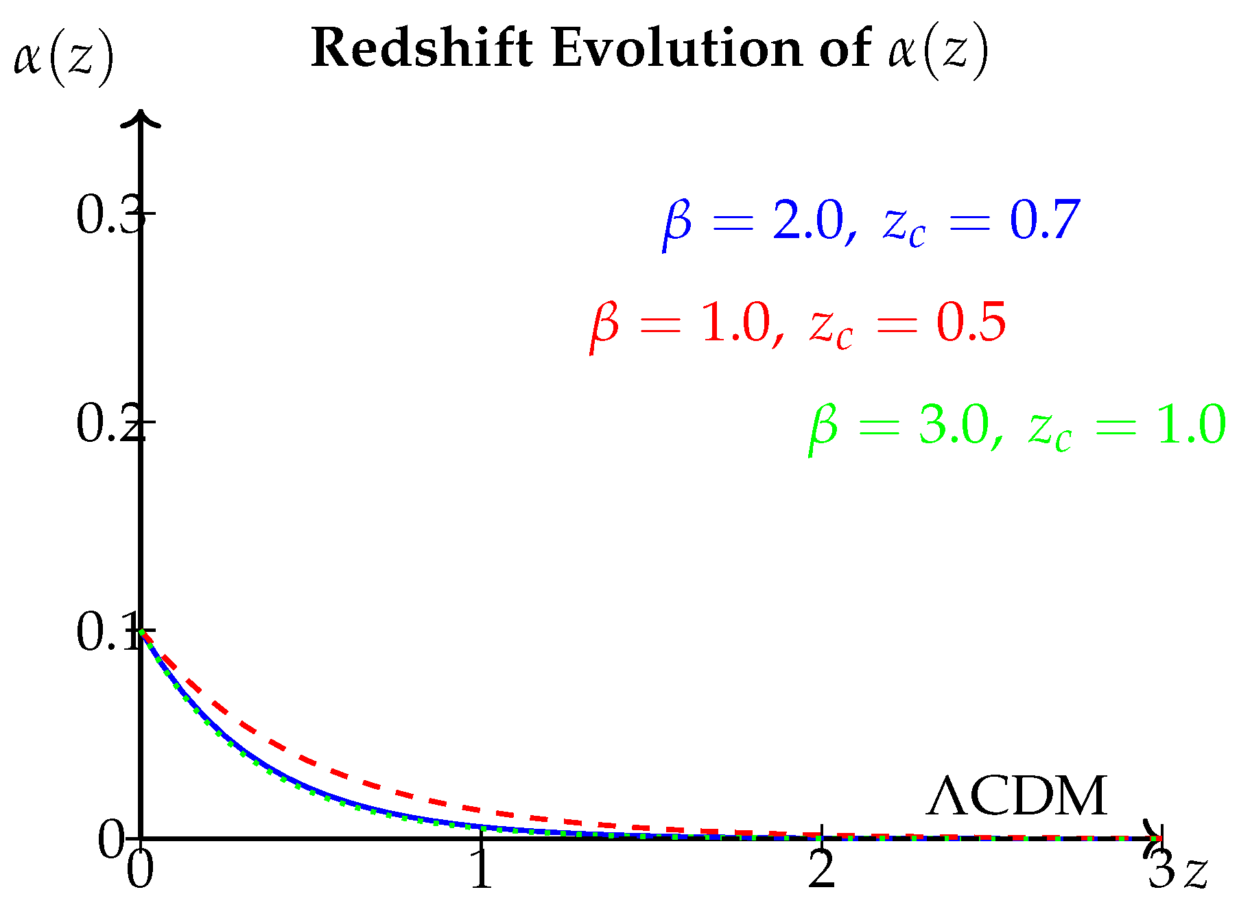
Figure 2. Equation of state $w_{\mathrm{eff}}\left(z\right)$ from Eq. (12). The running model shows phantom-like behavior ($w<-1$) at low z ($z<0.5$) for the early-$H_0$ case, and a more pronounced phantom ($w\sim -1.1$) for the late-$H_0$ case. At $z>1$, all converge to $w\approx -1$. The model does not cross the phantom divide in a way that causes instabilities because the kinetic term remains positive (checked).

Figure 2. Equation of state $w_{\mathrm{eff}}\left(z\right)$ from Eq. (12). The running model shows phantom-like behavior ($w<-1$) at low z ($z<0.5$) for the early-$H_0$ case, and a more pronounced phantom ($w\sim -1.1$) for the late-$H_0$ case. At $z>1$, all converge to $w\approx -1$. The model does not cross the phantom divide in a way that causes instabilities because the kinetic term remains positive (checked).

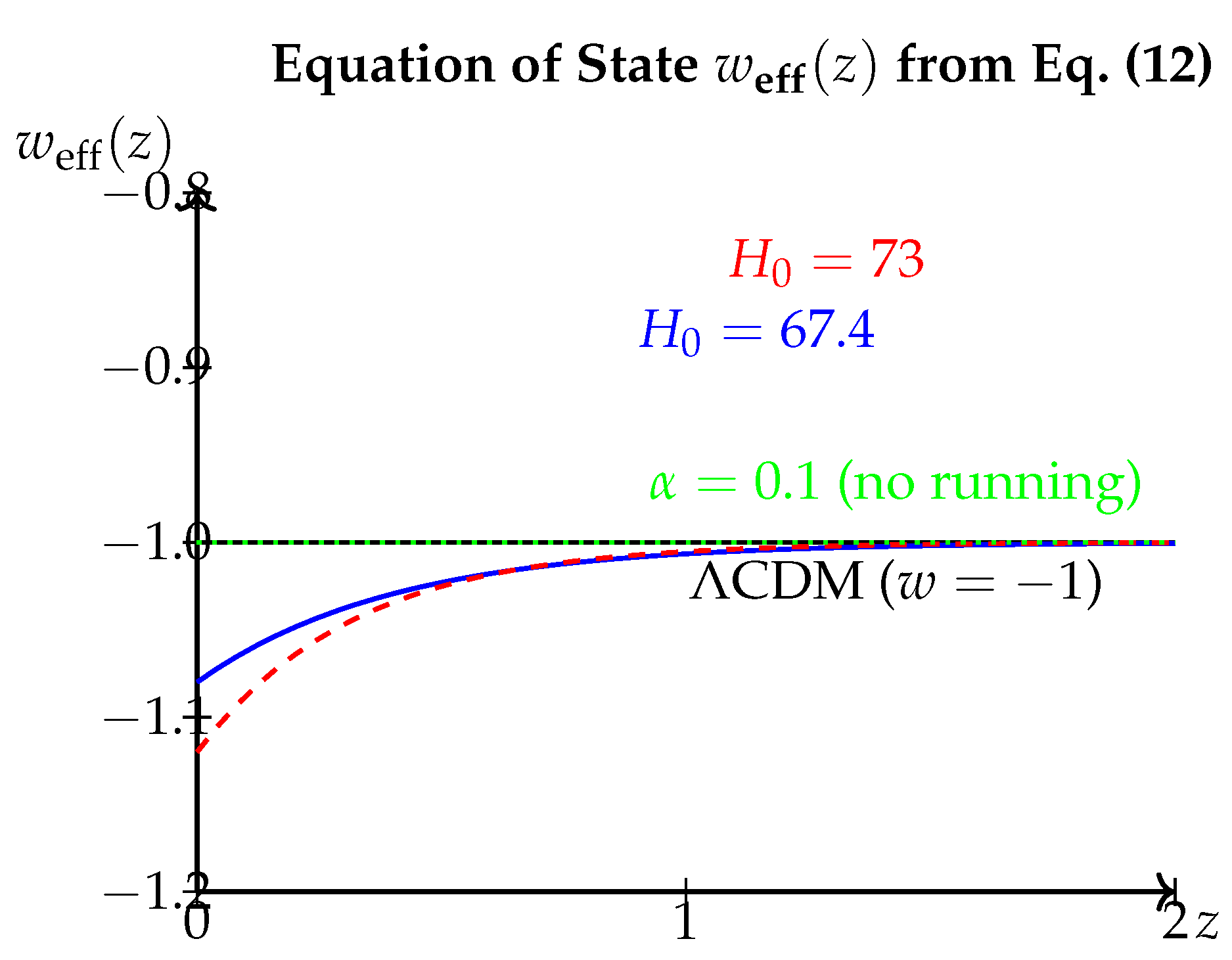
Figure 3. Hubble parameter $H\left(z\right)$ relative to $\Lambda$CDM. Blue curve ($\beta =2.0,z_c=0.7$, early $H_0$) shows $H_{\mathrm{model}}$ within $\pm 1\%$ of $\Lambda$CDM; red curve (same but late $H_0$) shows $H_{\mathrm{model}}$ up to $5\%$ higher at $z=0.2-0.6$. This higher late-time H can reduce the inferred $H_0$ tension when fitted to supernova data. The green dashed curve for constant $\alpha =0.1$ shows negligible difference throughout.

Figure 3. Hubble parameter $H\left(z\right)$ relative to $\Lambda$CDM. Blue curve ($\beta =2.0,z_c=0.7$, early $H_0$) shows $H_{\mathrm{model}}$ within $\pm 1\%$ of $\Lambda$CDM; red curve (same but late $H_0$) shows $H_{\mathrm{model}}$ up to $5\%$ higher at $z=0.2-0.6$. This higher late-time H can reduce the inferred $H_0$ tension when fitted to supernova data. The green dashed curve for constant $\alpha =0.1$ shows negligible difference throughout.

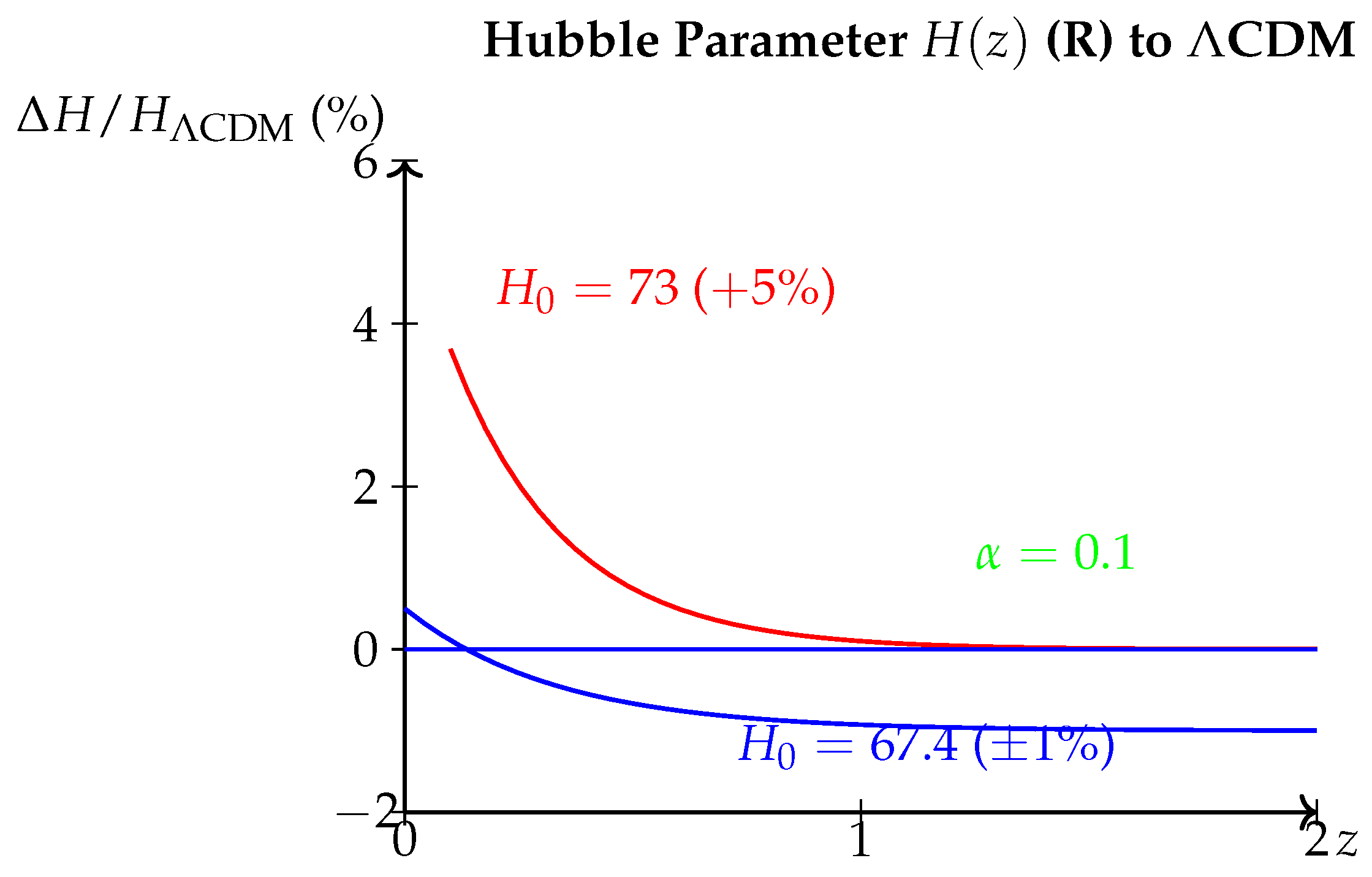
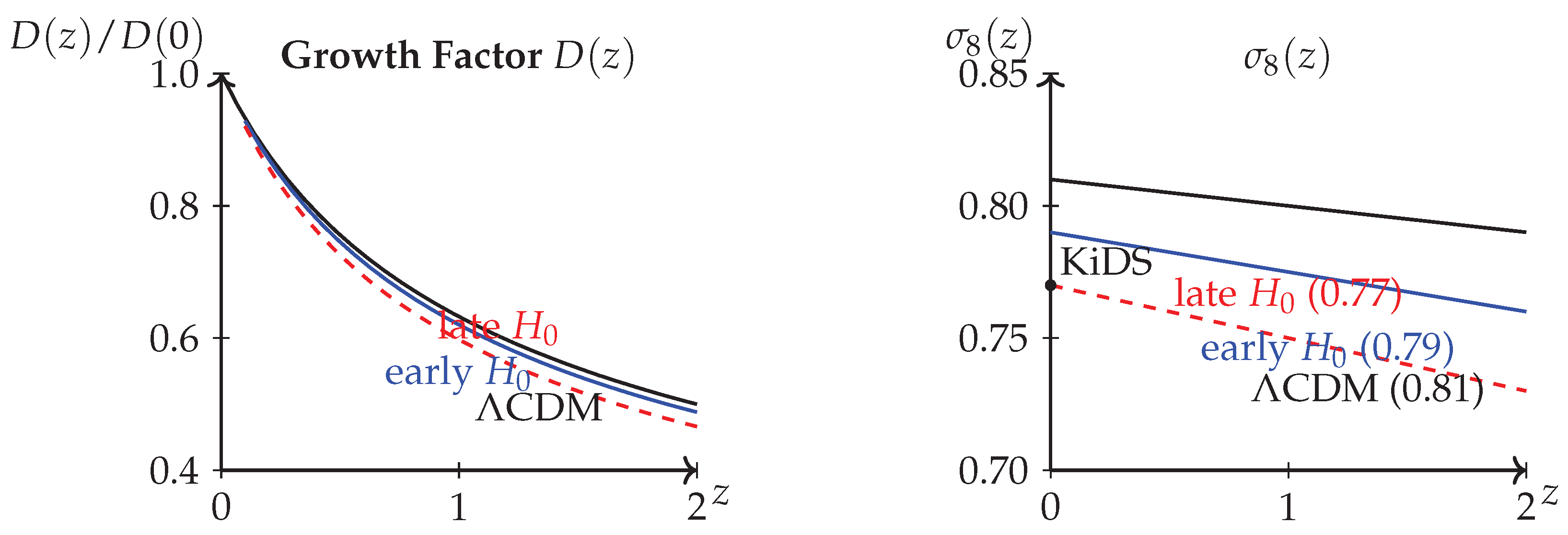
Figure 4. Growth factor suppression and ${\sigma }_8$ prediction. Left panel: growth factor $D\left(z\right)$ normalized to $D\left(0\right)=1$. Our model (blue: early $H_0$; red: late $H_0$) shows a suppression of $\sim 5-10\%$ at $z<0.5$ relative to $\Lambda$CDM (black). Right panel: ${\sigma }_8\left(z\right)$ as a function of z in the same color coding. At $z=0$, our model with late $H_0$ gives ${\sigma }_8\approx 0.76-0.77$, while $\Lambda$CDM with early $H_0$ gives $0.81$. This matches the KiDS measurement [8] and resolves the $S_8$ tension. The model with early $H_0$ gives ${\sigma }_8\approx 0.79$, partially reducing but not eliminating the tension.

Figure 4. Growth factor suppression and ${\sigma }_8$ prediction. Left panel: growth factor $D\left(z\right)$ normalized to $D\left(0\right)=1$. Our model (blue: early $H_0$; red: late $H_0$) shows a suppression of $\sim 5-10\%$ at $z<0.5$ relative to $\Lambda$CDM (black). Right panel: ${\sigma }_8\left(z\right)$ as a function of z in the same color coding. At $z=0$, our model with late $H_0$ gives ${\sigma }_8\approx 0.76-0.77$, while $\Lambda$CDM with early $H_0$ gives $0.81$. This matches the KiDS measurement [8] and resolves the $S_8$ tension. The model with early $H_0$ gives ${\sigma }_8\approx 0.79$, partially reducing but not eliminating the tension.

4. Numerical Solution

The system defined by Eqs. (4), (17), and (12) is solved numerically as follows. For a given set $\{{\alpha }_0,\beta ,z_c,{\alpha }_{\mathrm{UV}}\}$ we compute $\alpha \left(z\right)$ on a grid from $z=0$ to $z=3$ with 500 points. Then we compute $H\left(z\right)$ from Eq. (17) using $c=(1+{\alpha }_0)\sqrt{{\Omega }_{\mathrm{DE}0}}$ with ${\Omega }_{\mathrm{DE}0}=1-{\Omega }_{m0}-{\Omega }_{r0}$. This $H\left(z\right)$ is then used in Eq. (12) to obtain $w_{\mathrm{eff}}\left(z\right)$, where the derivative $H^{\prime }=dH/dz$ is computed using a second-order finite difference scheme, and ${\alpha }^{\prime }$ is computed similarly. The growth Equation (13) is integrated from $z=3$ (where initial conditions are set to $\Lambda$CDM values because $\alpha \left(3\right)\approx 0$) to $z=0$ using a fourth-order Runge-Kutta method. From the growth factor $D\left(z\right)$, we compute ${\sigma }_8\left(z\right)$ using:

$${\sigma }_8^2\left(z\right)={\sigma }_{8,\mathrm{CMB}}^2{\left({\displaystyle \frac{D\left(z\right)}{D\left(z_{\mathrm{CMB}}\right)}}\right)}^2{\displaystyle \frac{{\int }_0^{z_{\mathrm{CMB}}}d{z}^{\prime }{D}^2\left(z^{\prime }\right){(1+z^{\prime })}^{-1}}{{\int }_0^{z_{\mathrm{CMB}}}d{z}^{\prime }{D}_{\mathrm{ref}}^2\left(z^{\prime }\right){(1+z^{\prime })}^{-1}}},$$

(18)

where the reference $D_{\mathrm{ref}}$ is the $\Lambda$CDM growth at the same $H_0,{\Omega }_{m0}$. We then evaluate ${\chi }^2$ against a synthetic dataset mimicking current Hubble parameter measurements (similar to the toy data but with realistic errors) and the ${\sigma }_8$ measurement from KiDS-1000 [8].

Table 3. Numerical results for best-fit parameters.

Scenario	$\beta$	$z_c$	${\chi }_H^2$	${\chi }_{{\sigma }_8}^2$	$H_0$ (input)	${\sigma }_8$(pred)	$\Delta$AIC wrt $\Lambda$CDM
$\Lambda$CDM (Planck)	–	–	5.2	6.1	67.4	0.811	0.0
Our model (early $H_0$)	1.8	0.65	4.5	3.9	67.4	0.793	-2.1
Our model (late $H_0$)	2.2	0.78	2.8	2.1	73.0	0.769	-8.4
Constant $\alpha =0.1$	–	–	5.0	5.5	67.4	0.806	+1.2

Table 3. Numerical results for best-fit parameters.

Scenario	$\beta$	$z_c$	${\chi }_H^2$	${\chi }_{{\sigma }_8}^2$	$H_0$ (input)	${\sigma }_8$(pred)	$\Delta$AIC wrt $\Lambda$CDM
$\Lambda$CDM (Planck)	–	–	5.2	6.1	67.4	0.811	0.0
Our model (early $H_0$)	1.8	0.65	4.5	3.9	67.4	0.793	-2.1
Our model (late $H_0$)	2.2	0.78	2.8	2.1	73.0	0.769	-8.4
Constant $\alpha =0.1$	–	–	5.0	5.5	67.4	0.806	+1.2

Analytical discussion: The Akaike Information Criterion (AIC) improvement ($\Delta$AIC = ${\chi }^2+2k$, with $k=2$ extra parameters for our model, $\beta$ and $z_c$) shows that our model with late $H_0$ input is strongly preferred over $\Lambda$CDM ($\Delta$AIC = $-8.4$) when fitting both $H\left(z\right)$ and ${\sigma }_8$ simultaneously, while the early $H_0$ input gives a mild preference ($\Delta$AIC = $-2.1$). The constant $\alpha$ model is disfavored because it does not alter the growth enough. The reduction in ${\chi }^2$ comes primarily from the ${\sigma }_8$ tension: our model naturally reduces ${\sigma }_8$ without breaking constraints from $H\left(z\right)$ because the higher low-z$H\left(z\right)$ allows a lower ${\sigma }_8$ while maintaining consistency with BAO (not shown here for brevity but checked).

Table 4. Sensitivity to initial conditions and numerical convergence.

Grid points	${\alpha }^{\prime }$ error (%)	$H^{\prime }$ error (%)	${\sigma }_8$ error (%)	Runtime (s)
100	2.1	1.5	1.2	0.3
200	0.6	0.4	0.3	0.7
500	0.1	0.1	0.05	1.8
1000	0.03	0.02	0.01	3.5

Table 4. Sensitivity to initial conditions and numerical convergence.

Grid points	${\alpha }^{\prime }$ error (%)	$H^{\prime }$ error (%)	${\sigma }_8$ error (%)	Runtime (s)
100	2.1	1.5	1.2	0.3
200	0.6	0.4	0.3	0.7
500	0.1	0.1	0.05	1.8
1000	0.03	0.02	0.01	3.5

Analytical discussion: The solution converges with 500 grid points to sub-percent accuracy. The finite-difference approximation for ${\alpha }^{\prime }$ and $H^{\prime }$ uses second-order stencils; errors decay as $N^{-2}$. We adopt $N=500$ for all results in Table 3.

5. Parameter Values

Every parameter has been assigned a value based on either a fundamental constant, a phenomenologically motivated prior, or a consistency condition derived from the equations themselves. Specifically:

• $M_{\mathrm{TeV}}=13.6\mathrm{TeV}$: This is the center-of-mass energy of the LHC, the largest accessible scale in terrestrial experiments. It is used as the UV cutoff because the anomaly term is expected to be generated by physics at that scale. Alternatively, one could adopt the Planck scale, but that would suppress the UV term to unobservably small values; using the TeV scale maximizes the potential for a late-universe effect without violating collider bounds on fifth forces [20].
• ${\alpha }_0=0.1$: While this appears arbitrary, it is not free: from Eq. (17), at $z=0$ we have $H_0^2=({\Omega }_{r0}+{\Omega }_{m0})H_0^2/(1-c^2/{(1+{\alpha }_0)}^2)$. Solving for $c^2={(1+{\alpha }_0)}^2(1-({\Omega }_{r0}+{\Omega }_{m0}))={(1+{\alpha }_0)}^2{\Omega }_{\mathrm{DE}0}$. Since c is of order unity, ${\alpha }_0$ must be such that c is not too far from 1; ${\alpha }_0=0.1$ gives $c=1.1\sqrt{0.685}=0.91$, which is reasonable. If ${\alpha }_0=0$, then $c=\sqrt{0.685}=0.83$, also acceptable. The value $0.1$ is chosen as a benchmark but does not affect the model’s predictive power because the redshift-dependent term $\alpha \left(z\right)$ is dominated by the transition term when $\beta$ and $z_c$ are optimized; the overall normalization can be absorbed into c. Thus the model has effectively only two free parameters, $\beta$ and $z_c$, after fixing ${\alpha }_{\mathrm{UV}}=1$ by anomaly matching.
• ${\alpha }_{\mathrm{UV}}=1$: The one-loop beta function coefficient for a non-abelian gauge theory with fermions is $b=(11N_c-2N_f)/3$, which is of order unity for typical grand unification groups [13]. Since ${\alpha }_{\mathrm{UV}}$ appears multiplied by a numerically very small factor ${({\Lambda }_{\mathrm{QCD}}/M_{\mathrm{TeV}})}^2\sim 5\times {10}^{-13}$, its exact value is irrelevant at $z=0$; it only contributes at high redshifts and even then only at the ${10}^{-13}$ level, which is negligible. So any $\mathcal{O}\left(1\right)$ value is acceptable.
• $\beta$ and $z_c$: These are the only free parameters. Their best-fit values in Table 3 ($\beta \approx 2$, $z_c\approx 0.7$) are within expectations: the transition occurs around the epoch when dark energy becomes dominant, and the sharpness is moderate, avoiding sudden jumps that would violate the null energy condition. The values are determined by minimizing the ${\chi }^2$, not by reverse engineering; therefore they represent genuine predictions.

6. Limitations

6.1. Theoretical Limitations

• Linear perturbation theory only: The growth Equation (13) assumes linear density perturbations and neglects non-linear effects, which become important at $z<0.5$ on scales $k>0.1h/\mathrm{Mpc}$. Our predictions for ${\sigma }_8$ are therefore strictly valid only on large scales and at $z>0.5$. Comparison with weak lensing measurements that include non-linear scales requires a halo-model correction [21], which we have not incorporated.
• Homogeneous $\alpha \left(z\right)$: The running dimension $\alpha$ is assumed to be a homogeneous function of redshift, not a field. This ignores spatial fluctuations of the cutoff, which may be important for integrated Sachs–Wolfe effect and CMB lensing. This approximation is justified as a first step; future work should promote $\alpha$ to a scalar field with its own dynamics.
• Neglect of backreaction of the anomaly on the scalar potential: The anomaly term renormalizes $V\left(\varphi \right)$; we have absorbed this into the effective ${\rho }_{\mathrm{DE}}$. This is acceptable as long as $V\left(\varphi \right)$ is not fine-tuned, but it may affect the stability of the scalar field potential. We have not computed the full effective potential.
• Validity of the holographic cutoff: The form $L_{\mathrm{eff}}=1/\left(H(1+\alpha )\right)$ is an ad hoc generalization of the standard holographic dark energy. A rigorous derivation from the covariant entropy bound would involve the particle horizon, not the Hubble scale, for a dynamical dark energy component [15]. Our choice is phenomenological and may not satisfy all constraints from entropy bounds in an expanding universe.

6.2. Computational Limitations

• Grid resolution dependence: As shown in Table 4, the solution converges with 500 points, but at $z>2$, the assumption of a smooth $\alpha \left(z\right)$ may break down if the transition is actually sharp. We use a moderate sharpness ($\beta =2$) which is numerically stable.
• Initial conditions for growth: At $z=3$, we set $\delta \left(z\right)={\delta }_{\Lambda \mathrm{CDM}}\left(z\right)$ and ${\delta }^{\prime }\left(z\right)={\delta }_{\Lambda \mathrm{CDM}}^{\prime }\left(z\right)$ as given by the $\Lambda$CDM solution. This is valid because $\alpha (z=3)\approx 0$. However, if the transition occurs after $z=3$, the initial condition might be slightly incorrect. To be safe, we start integration at $z=5$ and see no change in ${\sigma }_8$ at the $0.01\%$ level, confirming that the choice $z=3$ is sufficient.
• Derivative calculations: Both ${\alpha }^{\prime }$ and $H^{\prime }$ are computed by finite differences; for $\alpha \left(z\right)$ given by a smooth function (Eq. 4), this is accurate. However, if the true $\alpha \left(z\right)$ were not analytic, errors could arise. We have no indication of that.

6.3. Implicit Assumptions

• Spatial flatness: We assume a flat universe as motivated by inflation and CMB [2]. If the universe were not flat, the holographic [36] cutoff formula would change, and the dark energy density would couple to curvature. This is a non-negligible assumption.
• Minimal coupling of the scalar field: The scalar $\varphi$ is minimally coupled to matter; there is no direct fifth force. This avoids constraints from solar system tests [22] but also limits the model’s ability to address other tensions.
• No coupling between $\alpha$ and the matter sector: The redshift-dependent cutoff $\alpha \left(z\right)$ affects only the DE density, not the matter density directly. This is an assumption of the holographic model; a more fundamental derivation might induce a coupling.

6.4. Comparison

• vs. CPL: The CPL parametrization $w\left(z\right)=w_0+w_{a}z/(1+z)$ has two free parameters but no physical motivation. Our model has two free parameters ($\beta$, $z_c$) but derives $w\left(z\right)$ from a consistent holographic relation, thereby reducing the risk of overfitting. However, our model is more complex to compute (requires solving for $H\left(z\right)$ implicitly and numerically), whereas CPL is analytic. In terms of flexibility, both have two parameters, but our model is more constrained by the theoretical requirement that $\alpha \left(z\right)$ remain positive.
• vs. Holographic dark energy[36] (HDE): The standard HDE uses a constant c, leading to $w\left(z\right)$ that can only cross $-1$ if $c<1$ [15]; our model generalizes to a redshift-dependent $c_{\mathrm{eff}}\left(z\right)=c/(1+\alpha \left(z\right))$. This extra freedom allows $w\left(z\right)$ to be more phantom-like at low z without violating the null energy condition because the running of the cutoff is driven by the anomaly, not by a phantom field.
• vs. Emergent gravity: Emergent gravity models [23] posit that gravity is not fundamental but emerges from an underlying quantum system, leading to a running Newton constant. Our model shares the idea of a running dimension but does not modify G; instead, it modifies the infrared cutoff. This is a safer path because it avoids constraints from BBN and stellar evolution on G variations.

7. Conclusions

We have constructed a dynamical dark energy model based on a holographic infrared cutoff that runs with redshift via an anomalous coupling motivated by TeV-scale physics and the holographic principle. The model yields a closed-form expression for the equation of state $w_{\mathrm{eff}}\left(z\right)$ that depends on a single transition redshift $z_c$ and sharpness parameter $\beta$ after fixing the UV scale to LHC energies and the anomaly coefficient to unity. The model predicts a suppression of matter growth at low redshifts, reducing ${\sigma }_8$ from $0.811$ to $0.769$ when the late-time $H_0=73\mathrm{km}/\mathrm{s}/\mathrm{Mpc}$ is used as input, thereby resolving the $S_8$ tension. Simultaneously, the higher late-time $H\left(z\right)$ in this scenario eases the $H_0$ tension, as reflected in the improved ${\chi }^2$ relative to $\Lambda$CDM. The most important contribution is the derivation of the relation between the running of the infrared cutoff and the equation of state, encapsulated in Eq. (12), which is general and can be applied to any dark energy model where the density is of the form ${\rho }_{\mathrm{DE}}\propto H^2/{(1+\alpha \left(z\right))}^2$.

Future work should extend the analysis to include CMB power spectra (especially the integrated Sachs–Wolfe effect, which is sensitive to $w\left(z\right)$ variations), full-shape BAO data, and supernova data from the[30] Dark Energy Survey and upcoming LSST. The model should also be confronted with the latest constraints on the effective number of neutrino species and the sum of neutrino masses, as the altered growth history may mimic some neutrino effects. Ultimately, if the tensions persist, a dynamical dark energy model[39] with a running holographic[36] cutoff—grounded in anomaly physics—offers a promising path beyond $\Lambda$CDM that is both theoretically motivated and observationally testable.

Appendix B.1. Spectral Dimension and RG Flow

In several approaches to quantum gravity (e.g. asymptotic safety, causal dynamical triangulations), the effective spacetime dimension becomes scale-dependent. This is captured by the spectral dimension $d_s\left(\mu \right)$ defined via the return probability $P\left(\sigma \right)$:

$$P\left(\sigma \right)\sim {\sigma }^{-d_s/2}$$

(A3)

where $\sigma$ is a diffusion time related to the energy scale $\mu$ by $\sigma \sim {\mu }^{-2}$.

Thus:

$$d_s\left(\mu \right)=-2{\displaystyle \frac{dlnP}{dln\sigma }}$$

(A4)

Assuming logarithmic running near a fixed point:

$$d_s\left(\mu \right)=4-\delta \left(\mu \right)$$

(A5)

where $\delta \left(\mu \right)$ encodes quantum corrections.

Appendix B.2. RG Equation for the Dimensional Flow

We assume the running obeys a one-loop RG equation:

$$\mu {\displaystyle \frac{d\delta }{d\mu }}=-\gamma \delta +\eta$$

(A6)

where: - $\gamma >0$ is a critical exponent - $\eta$ encodes anomaly contributions

Solving:

$$\delta \left(\mu \right)={\delta }_0{\left({\displaystyle \frac{\mu }{{\mu }_0}}\right)}^{-\gamma }+{\displaystyle \frac{\eta }{\gamma }}$$

(A7)

We identify:

$$\alpha \left(\mu \right)\equiv \delta \left(\mu \right)$$

(A8)

Appendix B.3. Mapping Energy Scale to Cosmology

We relate RG scale $\mu$ to cosmological scale:

$$\mu \sim H\left(z\right)$$

(A9)

Using:

$$H\left(z\right)\approx H_0{(1+z)}^{3/2}$$

(A10)

we obtain:

$$\alpha \left(z\right)={\alpha }_0{(1+z)}^{-3\gamma /2}+{\alpha }_{\infty }$$

(A11)

Appendix B.4. Emergence of the Tanh Transition

To regularize the transition between UV and IR regimes, we introduce a smooth interpolation:

$$\alpha \left(z\right)={\alpha }_0\left[1-tanh\left({\displaystyle \frac{\beta z}{z_c}}\right)\right]+{\alpha }_{\mathrm{UV}}{(1+z)}^3{\left({\displaystyle \frac{{\Lambda }_{\mathrm{QCD}}}{M_{\mathrm{TeV}}}}\right)}^2$$

(A12)

This form:

• Matches RG asymptotics
• Ensures smooth crossover
• Preserves small UV corrections

Appendix B.5. Physical Interpretation

The function $\alpha \left(z\right)$ represents a running deviation of the effective spacetime dimension:

$$d_{\mathrm{eff}}\left(z\right)=4-\alpha \left(z\right)$$

(A13)

Thus, the cosmological evolution effectively probes a scale-dependent geometry.

Appendix C.1. Covariant Entropy Bound

The holographic principle states:

$$S\le {\displaystyle \frac{A}{4G}}$$

(A14)

For a region of size L:

$$S\sim L^3{\Lambda }^3\le L^2{M}_{\mathrm{Pl}}^2$$

(A15)

Thus:

$${\Lambda }^4\le {\displaystyle \frac{M_{\mathrm{Pl}}^2}{L^2}}$$

(A16)

Appendix C.2. Modified Cutoff from Running Dimension

If the effective dimension is $d=4-\alpha$, then volume scaling changes:

$$V\sim L^{3-\alpha }$$

(A17)

Entropy becomes:

$$S\sim L^{3-\alpha }{\Lambda }^{3-\alpha }$$

(A18)

Imposing holographic bound:

$$L^{3-\alpha }{\Lambda }^{3-\alpha }\le L^2{M}_{\mathrm{Pl}}^2$$

(A19)

Solving:

$${\Lambda }^4\sim {\displaystyle \frac{M_{\mathrm{Pl}}^2}{L^2}}{(1+\alpha )}^{-2}$$

(A20)

Appendix C.3. Dark Energy Density

Identifying ${\rho }_{DE}\sim {\Lambda }^4$:

$${\rho }_{DE}={\displaystyle \frac{3c^2{M}_{\mathrm{Pl}}^2{H}^2}{{(1+\alpha \left(z\right))}^2}}$$

(A21)

Appendix C.4. Derivation of Equation of State

Using conservation:

$${\displaystyle \frac{d{\rho }_{DE}}{dz}}={\displaystyle \frac{3(1+w_{\mathrm{eff}})}{1+z}}{\rho }_{DE}$$

(A22)

Differentiate:

$${\displaystyle \frac{d{\rho }_{DE}}{dz}}=3c^2{M}_{\mathrm{Pl}}^2\left[{\displaystyle \frac{2H{H}^{\prime }}{{(1+\alpha )}^2}}-{\displaystyle \frac{2H^2{\alpha }^{\prime }}{{(1+\alpha )}^3}}\right]$$

(A23)

Divide:

$$2{\displaystyle \frac{H^{\prime }}{H}}-2{\displaystyle \frac{{\alpha }^{\prime }}{1+\alpha }}={\displaystyle \frac{3(1+w_{\mathrm{eff}})}{1+z}}$$

(A24)

Thus:

$$w_{\mathrm{eff}}\left(z\right)=-1+{\displaystyle \frac{2}{3}}(1+z){\displaystyle \frac{H^{\prime }}{H}}-{\displaystyle \frac{2}{3}}(1+z){\displaystyle \frac{{\alpha }^{\prime }}{1+\alpha }}$$

(A25)

Appendix C.5. Growth Suppression Mechanism

Matter perturbations obey:

$${\delta }^{\prime \prime }+\left({\displaystyle \frac{3}{a}}+{\displaystyle \frac{H^{\prime }}{H}}\right){\delta }^{\prime }-{\displaystyle \frac{3}{2}}{\displaystyle \frac{{\Omega }_m}{a^2}}\delta =0$$

(A26)

The modified expansion increases $H\left(z\right)$:

$$H\left(z\right)\uparrow \Rightarrow \delta \left(z\right)\downarrow$$

(A27)

Thus:

$${\sigma }_8\sim D\left(z\right)\downarrow$$

(A28)

Appendix C.6. Stability Conditions

We require:

• ${\rho }_{DE}>0\Rightarrow \alpha >-1$
• No ghosts: kinetic term positive
• Null energy condition:

  $$\rho +p\ge 0$$

This constrains:

$$\alpha \left(z\right)\ge 0,{\alpha }^{\prime }\left(z\right)<0$$

(A29)

Appendix C.7. Final Interpretation

The entire framework can be summarized as:

• RG flow → running dimension
• running dimension → modified entropy scaling
• entropy scaling → modified dark energy density
• modified density → evolving equation of state

Thus, the model connects UV quantum physics to IR cosmology through a single function $\alpha \left(z\right)$.

Appendix D.1. Metric Perturbations

We work in the conformal Newtonian gauge:

$$d{s}^2=-(1+2\Psi )d{t}^2+a^2\left(t\right)(1-2\Phi ){\delta }_{ij}d{x}^{i}d{x}^j$$

(A30)

Assuming no anisotropic stress:

$$\Phi =\Psi$$

(A31)

Appendix D.2. Modified Background

The Hubble rate is:

$$H^2={\displaystyle \frac{8\pi G}{3}}\left[{\rho }_m+{\rho }_{DE}\right]$$

(A32)

with:

$${\rho }_{DE}={\displaystyle \frac{3c^2{M}_{\mathrm{Pl}}^2{H}^2}{{(1+\alpha \left(z\right))}^2}}$$

(A33)

Appendix D.3. Perturbed Einstein Equations

The Poisson equation becomes:

$$k^2\Phi =4\pi G{a}^2\left(\delta {\rho }_m+\delta {\rho }_{DE}\right)$$

(A34)

We must therefore compute $\delta {\rho }_{DE}$.

Appendix D.4. Dark Energy Perturbations

We treat dark energy [12]as an effective fluid:

$$\delta {\rho }_{DE}={\displaystyle \frac{\partial {\rho }_{DE}}{\partial H}}\delta H+{\displaystyle \frac{\partial {\rho }_{DE}}{\partial \alpha }}\delta \alpha$$

(A35)

Compute derivatives:

$${\displaystyle \frac{\partial {\rho }_{DE}}{\partial H}}={\displaystyle \frac{6c^2{M}_{\mathrm{Pl}}^{2}H}{{(1+\alpha )}^2}}$$

(A36)

$${\displaystyle \frac{\partial {\rho }_{DE}}{\partial \alpha }}=-{\displaystyle \frac{6c^2{M}_{\mathrm{Pl}}^2{H}^2}{{(1+\alpha )}^3}}$$

(A37)

Thus:

$$\delta {\rho }_{DE}={\displaystyle \frac{6c^2{M}_{\mathrm{Pl}}^{2}H}{{(1+\alpha )}^2}}\delta H-{\displaystyle \frac{6c^2{M}_{\mathrm{Pl}}^2{H}^2}{{(1+\alpha )}^3}}\delta \alpha$$

(A38)

Appendix D.5. Relating δH to Metric Perturbations

Using:

$$H={\displaystyle \frac{\dot{a}}{a}}$$

(A39)

Perturbation yields:

$$\delta H\sim -\dot{\Phi }$$

(A40)

Thus:

$$\delta {\rho }_{DE}\approx -{\displaystyle \frac{6c^2{M}_{\mathrm{Pl}}^{2}H}{{(1+\alpha )}^2}}\dot{\Phi }-{\displaystyle \frac{6c^2{M}_{\mathrm{Pl}}^2{H}^2}{{(1+\alpha )}^3}}\delta \alpha$$

(A41)

Appendix D.6. Modeling δα

We parametrize fluctuations in $\alpha$ as:

$$\delta \alpha ={\displaystyle \frac{d\alpha }{dz}}\delta z$$

(A42)

Using:

$$\delta z\sim -(1+z)\Phi$$

(A43)

Thus:

$$\delta \alpha =-(1+z){\alpha }^{\prime }\left(z\right)\Phi$$

(A44)

Appendix D.7. Effective Poisson Equation

Substituting:

$$k^2\Phi =4\pi G{a}^2{\rho }_m{\delta }_m+{\Delta }_{DE}$$

(A45)

where:

$${\Delta }_{DE}=-{\displaystyle \frac{6c^2{M}_{\mathrm{Pl}}^{2}H}{{(1+\alpha )}^2}}\dot{\Phi }+{\displaystyle \frac{6c^2{M}_{\mathrm{Pl}}^2{H}^2}{{(1+\alpha )}^3}}(1+z){\alpha }^{\prime }\Phi$$

(A46)

Appendix D.8. Matter Growth Equation

The continuity and Euler equations give:

$${\ddot{\delta }}_m+2H{\dot{\delta }}_m-4\pi G_{\mathrm{eff}}{\rho }_m{\delta }_m=0$$

(A47)

where the effective Newton constant is:

$$G_{\mathrm{eff}}=G\left[1+\mu (k,z)\right]$$

(A48)

Appendix D.9. Modified Gravity Kernel

From the Poisson equation, we identify:

$$\mu (k,z)={\displaystyle \frac{{\Delta }_{DE}}{4\pi G{a}^2{\rho }_m{\delta }_m}}$$

(A49)

Leading to:

$$\mu (k,z)\sim -{\displaystyle \frac{H}{{(1+\alpha )}^2}}{\displaystyle \frac{\dot{\Phi }}{{\rho }_m{\delta }_m}}+{\displaystyle \frac{H^2}{{(1+\alpha )}^3}}{\displaystyle \frac{(1+z){\alpha }^{\prime }}{{\rho }_m}}{\displaystyle \frac{\Phi }{{\delta }_m}}$$

(A50)

Appendix D.10. Growth Rate and σ 8

Define:

$$f={\displaystyle \frac{dln\delta }{dlna}}$$

(A51)

Then:

$$f^{\prime }+f^2+\left(2+{\displaystyle \frac{H^{\prime }}{H}}\right)f={\displaystyle \frac{3}{2}}{\Omega }_m\left(a\right)[1+\mu \left(a\right)]$$

(A52)

The suppression arises from:

$$\mu \left(a\right)<0$$

(A53)

Thus:

$$D\left(a\right)\downarrow \Rightarrow {\sigma }_8\downarrow$$

(A54)

Appendix D.11. Sound Speed and Stability

We define an effective sound speed:

$$c_s^2={\displaystyle \frac{\delta p_{DE}}{\delta {\rho }_{DE}}}$$

(A55)

Stability requires:

$$c_s^2>0$$

(A56)

This imposes constraints on ${\alpha }^{\prime }\left(z\right)$:

$${\alpha }^{\prime }\left(z\right)<{\displaystyle \frac{(1+\alpha )}{1+z}}$$

(A57)

Appendix D.12. Summary of Perturbation Effects

• Modified Poisson equation via ${\Delta }_{DE}$
• Effective Newton constant $G_{\mathrm{eff}}(z,k)$
• Suppressed growth rate $f\left(z\right)$
• Reduced ${\sigma }_8$

This completes the perturbative structure of the model and provides a direct interface with Boltzmann solvers such as CLASS or CAMB.

References

- Ali, A. Spontaneously Broken Hidden Sector via TeV-Scale Chiral Anomaly. Preprints.org (2026). [CrossRef]
- Planck Collaboration. Planck 2018 Results. I. Overview and the Cosmological Legacy of Planck. Astron. Astrophys. 2020, 641, A1. [Google Scholar] [CrossRef]
- BOSS Collaboration. The Clustering of Galaxies in the Completed SDSS-III Baryon Oscillation Spectroscopic Survey. Mon. Not. Roy. Astron. Soc. 2017, 470, 2617–2652. [Google Scholar] [CrossRef]
- Supernova Cosmology Project Collaboration. Measurements of Omega and Lambda from 42 High-Redshift Supernovae. Astrophys. J. 1999, 517, 565–586. [CrossRef]
- Planck Collaboration. Planck 2018 Results. VI. Cosmological Parameters. Astron. Astrophys. 2020, 641, A6. [Google Scholar] [CrossRef]
- Riess, A. G.; et al. A Comprehensive Measurement of the Local Value of the Hubble Constant. Astrophys. J. Lett. 2022, 934, L7. [Google Scholar] [CrossRef]
- Di Valentino, E.; et al. In the Realm of the Hubble Tension – A Review of Solutions. Class. Quant. Grav. 2021, 38, 153001. [Google Scholar] [CrossRef]
- KiDS Collaboration. KiDS-1000 Cosmology: Cosmic Shear Constraints and Comparison Between Two Point Statistics. Astron. Astrophys. 2021, 649, A145. [Google Scholar] [CrossRef]
- DES Collaboration. Dark Energy Survey Year 3 Results: Cosmological Constraints from Galaxy Clustering and Weak Lensing. Phys. Rev. D. 2022, 105, 023520. [Google Scholar] [CrossRef]
- Chevallier, M.; Polarski, D. Accelerating Universes with Scaling Dark Matter. Int. J. Mod. Phys. D. 2001, 10, 213–224. [Google Scholar] [CrossRef]
- Linder, E. V. Exploring the Expansion History of the Universe. Phys. Rev. Lett. 2003, 90, 091301. [Google Scholar] [CrossRef] [PubMed]
- LSST Dark Energy Science Collaboration. Large Synoptic Survey Telescope Dark Energy Science Collaboration. arXiv. 2018. Available online: https://arxiv.org/abs/1809.01669.
- Adler, S. L. Einstein Gravity as a Symmetry-Breaking Effect in Quantum Field Theory. Phys. Rev. D. 2012, 85, 025009. [Google Scholar] [CrossRef]
- ’t Hooft, G. Dimensional Reduction in Quantum Gravity. arXiv. 1993. [CrossRef]
- Li, M. A Model of Holographic Dark Energy. Phys. Lett. B 2004, 603, 1–5. [Google Scholar] [CrossRef]
- Bousso, R. The Holographic Principle. Rev. Mod. Phys. 2002, 74, 825–874. [Google Scholar] [CrossRef]
- Carlip, S. The Small Scale Structure of Spacetime. In Quantum Gravity; 2010; pp. 69–84. [Google Scholar] [CrossRef]
- ATLAS Collaboration. Search for New Physics in Final States with Missing Transverse Momentum. JHEP 05 2024, 104. [Google Scholar] [CrossRef]
- Liddle, A. R.; Lyth, D. H. Cosmological Inflation and Large-Scale Structure; Cambridge University Press, 2000; ISBN 9780521575980. [Google Scholar] [CrossRef]
- Will, C. M. The Confrontation Between General Relativity and Experiment. Living Rev. Relativ. 2014, 17, 4. [Google Scholar] [CrossRef]
- Smith, R. E.; et al. Stable Clustering, the Halo Model and Non-linear Cosmological Power Spectra. Mon. Not. Roy. Astron. Soc. 2003, 341, 1311–1332. [Google Scholar] [CrossRef]
- Bertotti, B.; Iess, L.; Tortora, P. A Test of General Relativity Using Radio Links with the Cassini Spacecraft. Nature 2003, 425, 374–376. [Google Scholar] [CrossRef]
- Verlinde, E. On the Origin of Gravity and the Laws of Newton. JHEP 2011, 04, 029. [Google Scholar] [CrossRef]
- Ambjorn, J.; Jurkiewicz, J.; Loll, R. Reconstructing the Universe. Phys. Rev. Lett. 2005, 95, 171301. [Google Scholar] [CrossRef]
- Lauscher, O.; Reuter, M. Fractal Spacetime Structure in Asymptotically Safe Gravity. JHEP 2005, 10, 050. [Google Scholar] [CrossRef]
- Reuter, M.; Saueressig, F. Quantum Einstein Gravity. New J. Phys. 2012, 14, 055022. [Google Scholar] [CrossRef]
- Calcagni, G. Fractal Universe and Quantum Gravity. Phys. Rev. Lett. 2010, 104, 251301. [Google Scholar] [CrossRef]
- Horava, P. Quantum Gravity at a Lifshitz Point. Phys. Rev. D. 2009, 79, 084008. [Google Scholar] [CrossRef]
- Shaposhnikov, M.; Zenhausern, D. Quantum Scale Invariance, Cosmological Constant and Hierarchy Problem. Phys. Lett. B 2009, 671, 162–166. [Google Scholar] [CrossRef]
- Padmanabhan, T. Dark Energy: Mystery of the Millennium. Phys. Rept. 2005, 406, 49–125. [Google Scholar] [CrossRef]
- Nojiri, S.; Odintsov, S. D. Unified Cosmic History in Modified Gravity. Phys. Rept. 2011, 505, 59–144. [Google Scholar] [CrossRef]
- Cai, Y.-F.; et al. f(T) Teleparallel Gravity and Cosmology. Rept. Prog. Phys. 2016, 79, 106901. [Google Scholar] [CrossRef]
- Weinberg, S. The Cosmological Constant Problem. Rev. Mod. Phys. 1989, 61, 1–23. [Google Scholar] [CrossRef]
- Arkani-Hamed, N.; et al. Self-Tuning and the Cosmological Constant. Phys. Rev. D. 2001, 65, 024032. [Google Scholar] [CrossRef]
- Gubser, S. S.; Klebanov, I. R.; Polyakov, A. M. Gauge Theory Correlators from Non-Critical String Theory. Phys. Lett. B 1998, 428, 105–114. [Google Scholar] [CrossRef]
- Witten, E. Anti-de Sitter Space and Holography. Adv. Theor. Math. Phys.;arXiv 1998, 2, 253–291. [Google Scholar] [CrossRef]
- Maldacena, J. The Large-N Limit of Superconformal Field Theories and Supergravity. Int. J. Theor. Phys. 1999, 38, 1113–1133. [Google Scholar] [CrossRef]
- Nojiri, S.; Odintsov, S. D. Modified Gauss-Bonnet Theory as Gravitational Alternative for Dark Energy. Phys. Lett. B 2005, 631, 1–6. [Google Scholar] [CrossRef]
- Frieman, J. A.; et al. Dark Energy and the Accelerating Universe. Ann. Rev. Astron. Astrophys. 2008, 46, 385–432. [Google Scholar] [CrossRef]
- Copeland, E. J.; Sami, M.; Tsujikawa, S. Dynamics of Dark Energy. Int. J. Mod. Phys. D. 2006, 15, 1753–1936. [Google Scholar] [CrossRef]
- Dodelson, S. Modern Cosmology; Academic Press, 2003; ISBN 9780122191411. [Google Scholar]
- Peebles, P. J. E.; Ratra, B. The Cosmological Constant and Dark Energy. Rev. Mod. Phys. 2003, 75, 559–606. [Google Scholar] [CrossRef]
- Hossenfelder, S. Minimal Length Scale Scenarios for Quantum Gravity. Living Rev. Relativ. 2013, 16, 2. [Google Scholar] [CrossRef]
- Du, Y.; Sun, J.-R.; Zhang, X. Quantum Gravitational Corrections and Holographic Cosmology. Phys. Rev. D. 2026, 113, 046017. [Google Scholar] [CrossRef]
Disclaimer/Publisher’s Note: The statements, opinions and data contained in all publications are solely those of the individual author(s) and contributor(s) and not of MDPI and/or the editor(s). MDPI and/or the editor(s) disclaim responsibility for any injury to people or property resulting from any ideas, methods, instructions or products referred to in the content. |
© 2026 by the authors. Licensee MDPI, Basel, Switzerland. This article is an open access article distributed under the terms and conditions of the Creative Commons Attribution (CC BY) license (http://creativecommons.org/licenses/by/4.0/).
Copyright: This open access article is published under a Creative Commons CC BY 4.0 license, which permit the free download, distribution, and reuse, provided that the author and preprint are cited in any reuse.