

Submitted:
21 May 2026
Posted:
22 May 2026
You are already at the latest version
Abstract
We formulate the Single Monad Model and Duality of Time Theory as a conditional reconstruction framework based on completion and projection. Generative histories compose at one level, while observers access completed records at another. The central mathematical problem is therefore to determine which observable quotient is selected by completed-future tests, predictive sufficiency, stable records, phase compatibility, and geometric stabilization. The reconstruction has five linked layers. First, deterministic tests select the coarsest quotient preserving all tested completed futures, while stochastic tests select the predictive quotient, the minimal sufficient state for all future completed-test laws. Second, the algebraic-geometric envelope is made explicit: finitely presented histories give monoid algebras and representation schemes; completion is modeled by sheafification or reflective closure; and projection becomes, when descent hypotheses are satisfied, a quotient prestack, quotient stack, algebraic space, or coarse moduli functor. Third, real Hilbert dynamics selects complex phase: admissible imaginary units are skew-adjoint square roots of −Id in the Real commutant, and positive time orientation selects the nonzero-frequency complex structure J. Fourth, endpoint-stable records force the projection-sensitive action correction to be an endpoint cocycle, and compact phase additivity gives ∆θ ≡ Srec/\( \hbar \) (mod 2π). Fifth, nonstationary phase transport yields a coordinate-free obstruction spectrum for particle creation, while completion-delay bounds yield Lorentzian cones and, in smooth stabilized sectors, connection-induced Lorentzian readout.
Keywords:
dual time
; Single Monad Model
; algebraic geometry
; completion/projection
; sheafification
; reflective closure
; quotient prestack
; quotient stack
; moduli functor
; behavioral quotient
; predictive quotient
; variational selection
; predictive locality
; Real commutant
; positive frequency
; complex structure
; phase-balanced tensor product
; quantum networks
; stable records
; phase-action relation
; Bogoliubov transformation
; obstruction spectrum
; completion-delay cone
; connection geometry
; Lorentzian reconstruction
I. Foundational Architecture: Histories, Observation, and Selection
1. Introduction and Reconstruction Program
1.1. The Structural Problem
The mathematical foundations of physics normally begin with several structures already in place: a complex Hilbert space for quantum theory, a phase factor of the form for semiclassical amplitudes, an irreversible record structure for observation, and a Lorentzian spacetime geometry for relativistic readout. These objects are extremely successful, but their simultaneous presence raises a structural question. Are they independent primitives, or can some of them be understood as compatible outputs of a deeper architecture relating formation and observation?
We develop the second possibility. We do not attempt to replace established quantum mechanics, quantum field theory, or relativity. Instead, we isolate a conditional reconstruction scheme in which familiar structures are assigned distinct roles in a single pipeline. Our basic move is to separate a level of admissible generative histories from a level of completed observable records. The completion/projection interface between these levels is then used to organize observable irreversibility, phase, action, particle creation, and geometric readout.
The word “time” in the Duality of Time Theory (DTT) is therefore not used here to mean a second coordinate time in spacetime. The distinction is functional and operational. There is a generative ordering or composability of histories, and there is an observable ordering of completed records. The physical temporal flow accessed by observers belongs to the second layer. The hidden generative level supplies admissible formation histories, but it is not directly identical with the measured time coordinate.
1.2. Algebraic-Geometric Scope and Interdisciplinary Role
We intentionally work across disciplines, but the algebraic-geometric component has a precise role. We do not assume that every state object in the theory is a scheme, nor do we use stack language as a metaphor for hidden variables. Instead, we ask what must be true when histories, completion data, record equivalences, and phase choices vary in families. In that setting the functor-of-points viewpoint, sheafification, reflective subcategories, quotient prestacks, quotient stacks, algebraic spaces, and moduli functors provide natural tests of whether a proposed observer-level quotient is stable under base change and descent.
This is why the algebraic-geometric layer is placed near the beginning of the reconstruction. It functions as a consistency envelope for completion and projection before the later operator-theoretic, record-theoretic, and Lorentzian modules are interpreted physically. The representation schemes of finitely presented history monoids encode algebraic families of admissible generative actions; sheafification and reflective closure model completed records; quotient stacks retain stabilizer and gluing data that a coarse pointwise quotient may erase; and descent failures become mathematical obstructions to treating a proposed projection as an algebraic observable quotient. Thus the algebraic-geometric material is not an isolated appendix to a physics proposal. It supplies the family-level language in which the central selection problem can be formulated and checked.
1.3. The Main Reconstruction Chain
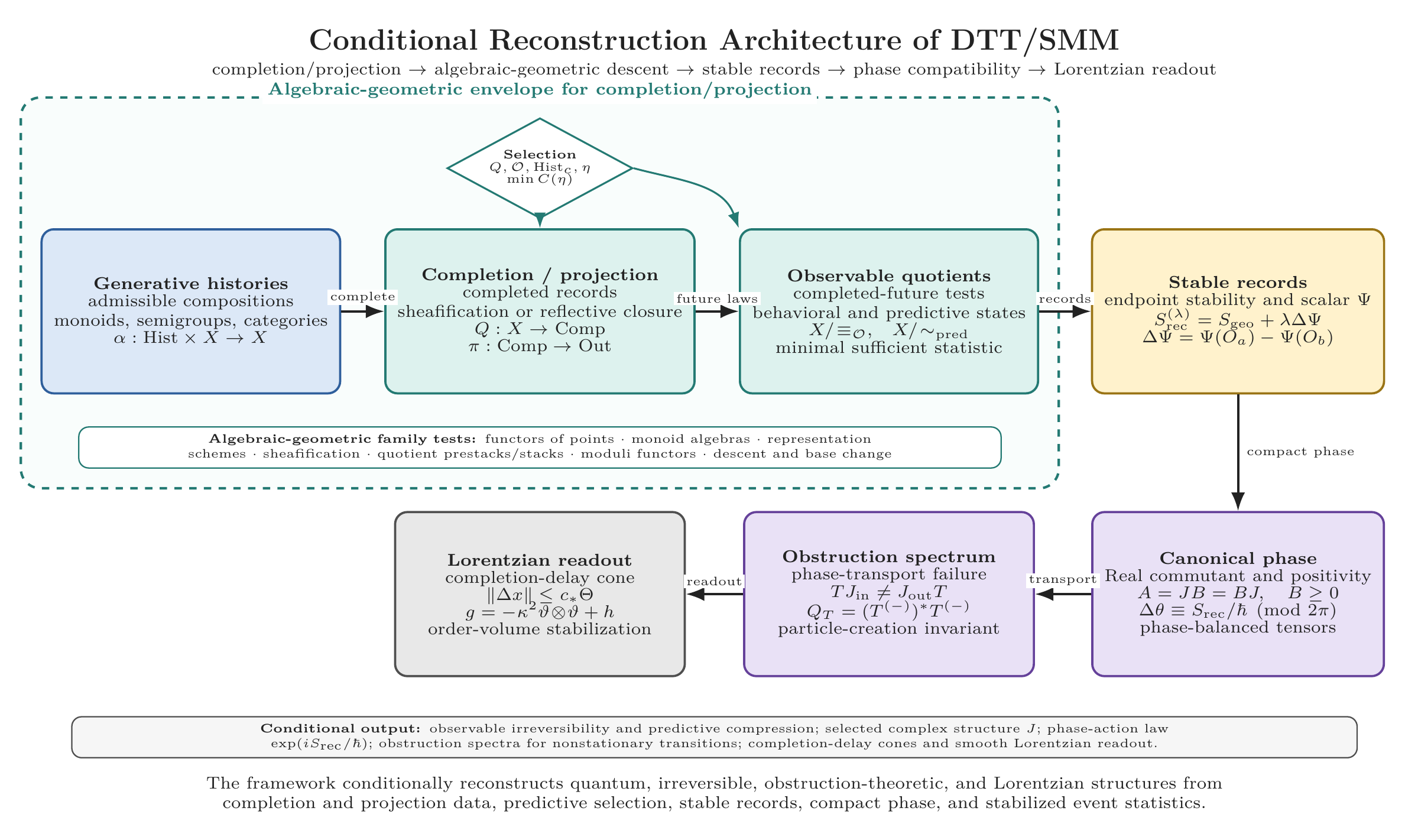
We organize the reconstruction around the chain
The arrows in this chain are not all of the same logical kind. Some are definitions, some are structural principles, some are theorem-level consequences, and some are reconstruction protocols. A central purpose of our formulation is to make those statuses explicit.
At the first stage, generative histories are modeled by monoids, semigroups, categories, or related process structures acting on a generative state space. At the second stage, completion and observation are represented by maps or functors that produce completed records. At the quotient-selection stage, completed-future tests identify exactly those generative distinctions that have no operational effect; in probabilistic models this becomes the predictive quotient, the minimal sufficient state for all future completed test statistics. At the third stage, record stability is imposed; this is where observable irreversibility, memory, and predictive compression enter. At the fourth stage, stable records carry an additive action variable, compact phase converts that variable into a phase modulo , and phase-balanced composition identifies independently selected imaginary units when composite complex systems are formed. At the fifth stage, nonstationary transitions between stationary phase structures, or phase mismatches in network composition, are measured by transport or balancing obstructions. At the geometric stage, bounded completed propagation supplies a delay cone , its smooth lift supplies a connection-induced Lorentzian metric, and stabilized event statistics supply the order and volume data required for manifoldlike reconstruction.
Principle 1.1
(Reconstruction before primitive insertion). The framework aims to reconstruct or reformulate complex phase, irreversible records, particle-production data, and Lorentzian readout from explicit input layers rather than inserting them as unrelated primitives.
Figure 1 condenses this chain into the navigation diagram used throughout the reconstruction.
1.4. Main Results and Theorem-Level Contributions
We separate theorem-level conclusions from principles, interpretations, and open selection problems. Our main formal contributions are the following.
- (R1)
- Observable semigroup descent and behavioral quotient selection. If a history action is compatible with the observed-record map, then histories descend to observable dynamics; if the generative dynamics is invertible but the quotient is many-to-one, the observable dynamics may be irreversible. For a fixed completion map, complete-future class, and operational test family, Theorem 3.13 shows that the selected observable state space is the coarsest quotient preserving all tested completed futures.
- (R2)
- Predictive quotient as minimal sufficient observable state. In stochastic realizations, Theorem 3.18 replaces equality of test outcomes by equality of future completed-test laws. The resulting predictive quotient is the minimal sufficient state for the specified future statistics, while Conjecture 3.20 formulates the remaining choice of test family as a variational predictive-selection problem.
- (R3)
- Algebraic-geometric envelope of completion/projection. Propositions 4.4, 4.7, and 4.10 identify the algebraic-family version of the framework: histories may be represented by monoid algebras and representation schemes, completion by sheafification or reflective closure, and observable projection by quotient prestacks, quotient stacks, algebraic spaces, or coarse moduli functors when the required descent and representability hypotheses hold.
- (R4)
- Real-commutant reconstruction of complex phase. Theorems 6.3, 6.13, and 6.15 show that, for real orthogonal dynamics, admissible imaginary units are the skew-adjoint square roots of in the Real commutant and that a positive time orientation selects the nonzero-frequency complex structure J in the relevant positive-energy sector.
- (R5)
- Phase-balanced composition and network operationality. Proposition 6.21 identifies the real form of the complex tensor product as a phase-balanced quotient. Theorem 6.26 then interprets source-independent real-versus-complex network violations as certificates of a shared transported phase, not merely as a notational preference for complex scalars.
- (R6)
- Stable-record phase-action law. Theorem 7.5 proves that endpoint-stable record closure forces the projection-sensitive action correction to be an endpoint cocycle. Theorem 7.8 then converts the additive record action into the compact phase law inside a calibrated protocol class.
- (R7)
- Obstruction spectra and Lorentzian readout. Theorem 9.6 reformulates particle creation as obstruction to transporting the selected phase structure. Theorems 11.6, 12.1, 12.3, and 13.8 then connect completion-delay bounds to Lorentzian cones, smooth connection-induced metrics, universal limiting speed, and order-volume reconstruction in stabilized manifoldlike sectors.
These results are not asserted as unconditional derivations of all physical dynamics. They are conditional rigidity and reconstruction statements: once the named input layers are supplied, the corresponding quotient, phase, action, obstruction, and readout structures follow.
1.5. A minimal Working Model
Before the full theorem chain is developed, it is useful to keep in mind the smallest schematic realization of the framework. One begins with a generative state space X carrying admissible histories. Completion sends X to completed records . A specified operational family defines the deterministic behavioral quotient ; in stochastic realizations it defines the predictive quotient , whose elements are minimal sufficient states for future completed test statistics. A stable record sector then carries an endpoint scalar , which in predictive models can be chosen as a monotone predictive-information functional, an additive record action , and a compact phase increment . In stationary Hilbert realizations, positive real dynamics selects J; in composite systems, phase-balanced tensoring identifies independently selected J operators as one shared scalar i; in nonstationary transitions, failure to transport this selected J gives the obstruction spectrum.
This minimal model is not a substitute for the later theorems. Its purpose is to show how the pieces fit before technical machinery is introduced. Figure 2 gives a compact schematic of this minimal working model.
1.6. Core Innovations
Our novelty claim is not that every mathematical ingredient is new. Many ingredients are standard: monoid actions, quotient maps, sheaves, quotient stacks, real Hilbert spaces, spectral theory, Weyl algebras, quasifree states, Bogoliubov transformations, causal order, and volume reconstruction. Our contribution is the architecture in which these ingredients are assigned compatible roles, together with the conditional rigidity results listed above. The main distinctive elements are the following.
- (I1)
- Generative-observational separation. Observable time is separated from the primitive generative ordering used to describe formation. The observed record order is not assumed to expose the full chronology of the generative history.
- (I2)
- Behavioral and predictive quotient selection. Projection is not allowed to remain an arbitrary many-to-one map. Once a completion map, a class of complete future histories, and a family of observer-level tests are specified, the observable quotient is defined as the coarsest quotient preserving all tested completed futures. In stochastic models the same idea becomes a predictive quotient: observable states are minimal sufficient states for future completed test statistics.
- (I3)
- Variational predictive selection. The framework does not yet derive nature’s test family from first principles, but it recasts that gap as a precise optimization problem: among all statistics that preserve the relevant future completed-test laws and support stable records, the physically realized observable presentation should minimize retained predictive complexity or redundancy.
- (I4)
- Algebraic-geometric envelope. Under finite-presentation and descent hypotheses, the completion/projection layer can be represented through functors of points, monoid algebras, semigroup schemes, representation schemes, sheafification, quotient prestacks, quotient stacks, and moduli functors.
- (I5)
- Intrinsic phase selection. Given a real Hilbert representation, the possible imaginary units are not an informal choice. They are the skew-adjoint square roots of in the Real commutant. For positive time-oriented flows, positivity selects a unique nonzero-frequency element of this parameter space.
- (I6)
- Stable-record phase-action reconstruction. Endpoint-stable record closure forces the allowed projection-sensitive action correction to be an endpoint cocycle. Compact phase additivity then turns the additive record variable into the usual phase law.
- (I7)
- Phase-balanced network composition. The real form of a complex tensor product is not the ordinary real tensor product but the quotient identifying the selected local phase operators. Source-independent real-versus-complex network tests therefore probe whether independently prepared systems share a transported J.
- (I8)
- Obstruction-spectrum particle creation. Bogoliubov coefficients are coordinate representations of a basis-free obstruction. The invariant occupation data are encoded by the spectral measure of .
- (I9)
- Lorentzian readout from completion delay and stabilized order-volume. The geometric sector is not assumed at the generative level. A local propagation budget and completion-delay law first yield an observer-level cone; in the smooth lift this becomes a connection-induced Lorentzian metric, and in manifoldlike regimes stabilized order-volume data reconstruct the effective geometry.
1.7. Conditional Status and Limits of the Reconstruction
Our claims are deliberately conditional. This conditional status is part of the mathematical design: each reconstruction theorem states which input layer is required and what fails if that layer is weakened. We do not derive the full Standard Model, the Born rule, interacting quantum field theory, gravitational field equations, or the numerical SI value of ℏ. We also do not claim that every physical system must satisfy DTT/SMM principles. The statements below have the following form: if a system admits the specified histories, completion/projection data, stable-record closure, compact phase calibration, positive real dynamics, phase-sharing rules, and manifoldlike stabilization, then the corresponding phase, action, obstruction, and geometric structures follow.
Discussion 1.2
(What is not claimed). We should not be read as offering an unconditional derivation of all physical dynamics. We present a constraint and reconstruction architecture. We make the input layers visible and then prove what those layers force. A different completion map, a different family of operational tests, a different treatment of zero modes, a different descent condition, or a different stabilization interface changes the resulting observable theory. This is why we use the introduction, dependency tables, theorem labels, and open-problem section to distinguish definitions, principles, theorem-level consequences, conjectures, and interpretations.
1.8. The Selection Problem as the Central Open Problem
Our main mathematical modules are consistency and reconstruction theorems. They show what follows from stated inputs. The central open problem is therefore not merely to write down projections or stable records; it is to identify which completion maps, operational tests, predictive state variables, stable-record protocols, compact phase calibrations, phase-sharing mechanisms, and stabilization interfaces are physically selected.
This selection problem is the point at which the framework becomes empirically and model-theoretically meaningful. A many-to-one projection can always be invented. The task is to determine which projection is selected by the available operational tests, when that quotient coincides with a minimal sufficient predictive state, which observables are retained because they preserve future completed-test statistics, and which record variables remain stable under all completed future continuations. In Section 3.6 this is sharpened into a variational selection principle: the realized observable presentation is selected as a minimal prediction-preserving presentation. Table 1 records the load-bearing inputs and the outputs they support. Figure 3 summarizes the dependency graph for the main reconstruction modules.
1.9. What Is Reconstructed and What Is Imported
A reconstruction framework is clearest when it distinguishes outputs from calibrations and external physical inputs. Table 2 gives the status of the principal structures used below. The table also prevents a common misunderstanding: we reconstruct the form and uniqueness of several structures inside specified protocol classes; we do not claim to derive every empirical constant or every physical law from no input.
1.10. Reconstruction, Derivation, and Translation
We use three kinds of language. A result is called a reconstruction when a familiar structure is recovered from stated inputs. It is called a derivation only when it follows directly from definitions and hypotheses. It is called a translation when a standard construction is placed into the DTT/SMM architecture without claiming mathematical novelty for the construction itself.
For example, Stone’s theorem is not new; its role here is to support the Real-commutant reconstruction of the complex structure from real positive dynamics. The Shale criterion is not new; its role here is to mark the Fock-implementability boundary of the obstruction operator. Order-volume reconstruction is not new; its role here is to identify the stabilized observable data required for Lorentzian readout.
1.11. The Focused Mathematical-Physics Core
Inside the broader DTT/SMM architecture lies a focused mathematical-physics core. This core is deliberately narrower than the full program. It does not attempt to derive measurement probabilities, interacting field theory, gravity, or the numerical laboratory value of Planck’s constant. It asks a sharper question: given real positive dynamics, endpoint-stable records, and compact phase, which complex phase structure and which action-phase law are compatible with those data?
The answer is a three-layer rigidity statement:
Equivalently,
The first statement is operator-theoretic: the imaginary unit is not postulated but selected as a real orthogonal complex structure. The second is record-theoretic: the action correction is forced by endpoint-stable concatenation. The third is metrological: the compact character of the additive record variable fixes the action-per-radian conversion constant inside a calibrated protocol class.
Particle creation and Lorentzian reconstruction are downstream of this core. Particle creation measures obstruction to transporting the selected phase structure through a nonstationary real symplectic transition. Lorentzian readout first appears through completion-delay cones, and continuum geometry is recovered only after observable event records stabilize enough to supply order and volume data.
1.12. Methods and Standing Assumptions
We use standard tools from monoid actions, category theory, sheaf theory, quotient stacks, real Hilbert spaces, direct integrals, compact representation theory, Weyl-CCR quantization, quasifree states, Bogoliubov transformations, and order-volume reconstruction. Algebraic-geometric statements are made under finite-presentation, representability, quotient-existence, and descent assumptions. Operator-theoretic statements assume the usual domain compatibility for unbounded generators. Physical interpretations are downstream readings of the mathematical structures rather than additional hidden assumptions.
2. Claim Status, Ontological Principles, and Temporal Roles
2.1. Claim-Status Discipline
Because DTT/SMM combines interpretation with theorem-bearing mathematics, we use a claim-status discipline.
| Label | Meaning we use here |
| Principle or Postulate | Structural commitment fixing the explanatory direction or the input class. |
| Definition | Formal mathematical object used in the theorem chain. |
| Theorem, Proposition, Corollary | Result proved from stated assumptions. |
| Remark, Discussion, Example | Interpretation, explanation, comparison, or illustration. |
| Conjecture, Question | Mathematically meaningful direction not proved here. |
Definition 2.1
(Claim-status hierarchy). A claim has theorem status only when it is a consequence of stated definitions and hypotheses. A claim has principle status when it fixes a structural input or explanatory direction. A claim has interpretive status when it explains the meaning of a formal result without adding a new theorem.
Remark 2.2
(Why this matters). The framework would be weaker if ontology, formal definitions, and theorem-level consequences were mixed without distinction. The goal is to let the interpretation motivate precise structures, not to disguise the interpretation as proof.
2.2. Foundational Principles
Principle 2.3
(Generative/observable separation). There is a generative level of admissible histories and an observable level of completed records. Observation accesses completed records, not the entire hidden chronology of their generation.
Principle 2.4
(Completion). A generative history becomes observable only after a completion operation. Completion may include stabilization, closure, redundancy, coarse graining, environmental selection, or another physical procedure that produces a record accessible to observation.
Principle 2.5
(Projection). Observable records generally retain only a quotient of the generative information. Distinct generative histories may have the same completed observable record.
Principle 2.6
(Record stability). Observable physics is formulated in terms of stable record sectors. A record is stable relative to a protocol when it remains identifiable under the completion and observational procedures of that protocol.
Principle 2.7
(Phase/readout separation). Compact recurrence and Lorentzian causal readout belong to different structural roles. Compact sectors support phase, whereas hyperbolic sectors support causal split readout. They may be related inside a larger architecture, but they should not be collapsed into one invariant quadratic geometry on a nontrivial irreducible compact sector.
2.3. The Single Monad Model as Interpretation
The Single Monad Model (SMM) supplies the conceptual motivation for a single generative source whose observable multiplicity appears only after completion/projection. We use that motivation in a mathematically restrained way. We do not require the detailed cosmological or metaphysical commitments of earlier SMM writings. We extract the structural content relevant to reconstruction: admissible histories, completion, projection, stable records, compact recurrence, and observer-level geometry.
Discussion 2.8
(Mathematical dependence on SMM). The formal results below depend on the existence of the stated mathematical data, not on acceptance of an independent metaphysical thesis. The SMM interpretation explains why such data are natural in this program. The theorems require the data themselves.
2.4. Temporal Role Separation
The framework uses several temporal roles that should not be confused.
Definition 2.9
(Temporal roles). A DTT/SMM model may involve:
- (T1)
- a generative composition parameter or ordering on histories;
- (T2)
- a completion or stabilization relation determining when a record is observable;
- (T3)
- an observable record order or event precedence relation;
- (T4)
- a stationary flow parameter t in a real Hilbert realization;
- (T5)
- a phase parameter on compact sectors;
- (T6)
- a proper-time or Lorentzian interval parameter reconstructed in a manifoldlike regime.
These roles may be related, but they are not identical by definition.
Remark 2.10
(DTT is not ordinary two-time physics). The distinction between generative and observable time is not a claim that spacetime has two coordinate-time dimensions. It is a separation between the order of formation and the order of completed records.
3. Theorem Layer 0: Operational Selection of Observable Dynamics
Roadmap. This layer turns the generative/observable separation into an operational selection rule. It starts with monoid actions of admissible histories, descends complete histories through an observable quotient, and then sharpens the quotient to behavioral and predictive equivalence. The output is a minimal observable state space for the chosen family of completed-future tests.
3.1. Admissible Histories as Actions
Definition 3.1
(History monoid). A history monoid is a monoid whose elements represent admissible generative histories or history fragments. The identity element e represents the null history, and multiplication represents concatenation or composition.
Definition 3.2
(Generative state action). Let X be a generative state space. A history action is a map
written or , such that and for all and .
The use of a monoid rather than a group is intentional. A generative history may have a well-defined composition law without every fragment being invertible inside the chosen admissible class. When an invertible generative dynamics is intended, one may use a group action. The observable quotient can still be irreversible even if the generative action is invertible.
Definition 3.3
(Complete histories). A complete-history class is a subset containing those history fragments that are admissible as completed future continuations for the observational protocol under consideration. In many models ; in others it is a distinguished submonoid or a domain of histories satisfying boundary, stabilization, or closure conditions.
3.2. Completion and Observation
Definition 3.4
(Completion data). Completion-observation data consist of a generative state space X, a completed-record space , a completion map
and, when needed, an observable projection
The composite is the observed record map.
In a minimal deterministic model, Q is an ordinary map. In stochastic, categorical, or sheaf-theoretic models, Q may be a Markov kernel, functor, relation, sheafification morphism, or other completion operation. The theorem below is stated in the deterministic setting because it captures the essential quotient mechanism.
Definition 3.5
(Compatibility with observation). Let . A history is compatible with the observable quotient if
for all . The action is compatible if every is compatible.
Theorem 3.6
(Observable semigroup descent). Suppose acts on X and the observable map is surjective. If the action is compatible with ρ, then each induces a well-defined observable map
and is a monoid action of on . If the generative action is invertible but some is not injective, then exact generative reversibility descends to irreversible observable dynamics.
Proof.
Well-definedness follows directly from compatibility: if , then . The identity history induces the identity map because . For ,
Thus the descended maps form a monoid action. If the maps on X are invertible but a quotient identifies distinct generative states, the induced map on may fail to be injective; then the observable evolution has lost information even though the generative evolution has not. □
Example 3.7
(A quotient-irreversible shift). Let , where each is countably infinite, and let send all elements of to the label n. Choose a bijection that maps bijectively onto one countable half of and maps bijectively onto the complementary half of . Then is invertible on X, but the descended observable map is
which is surjective and not injective. Thus an invertible generative step can appear as an irreversible coarse observable step.
3.3. Entropy and Relative Entropy Under Projected Dynamics
The preceding theorem is purely set-theoretic. In probabilistic or quantum realizations, observable irreversibility often appears as monotonicity of an information functional under a reduced channel. The following standard proposition records the version needed here.
Proposition 3.8
(Data-processing arrow for reduced channels). Let Φ be a completely positive trace-preserving map on density matrices. If σ is a faithful stationary state, , then
for every state ρ, where D is quantum relative entropy. If, in finite dimension, Φ is unital, then the von Neumann entropy satisfies
For a semigroup with invariant σ, the function is nonincreasing.
Proof.
The first statement is the data-processing inequality for quantum relative entropy. If is unital on a d-dimensional algebra, the maximally mixed state is invariant and
Applying data processing to gives the entropy inequality. For the semigroup statement, write and apply data processing from time s to time t. □
Remark 3.9
(Entropy scope). Ordinary entropy is not monotone under arbitrary non-unital dynamics. The safe arrow is relative entropy to a faithful stationary reference state. Infinite-dimensional versions require modular-domain control and are not assumed without additional hypotheses.
3.4. Behavioral Selection of the Observable Quotient
Projection alone is not a physical selection principle. Many inequivalent many-to-one maps can produce irreversible effective dynamics. The first signature theorem of the framework is therefore operational rather than metaphysical: once a completion map, a complete-future class, and a test family are fixed, the observable quotient is the coarsest quotient preserving all tested completed futures. This rule specifies which distinctions are erased and which are retained.
Definition 3.10
(Operational test family). Let be a specified family of observer-level tests on completed states. Each test is a map
where is the outcome set of that test. The family may include ordinary coarse outcomes, calibrated record variables such as , phase readouts modulo , stabilization horizons, or event-side order/volume observables. In an empirical realization, must be stated together with resolution tolerances.
Definition 3.11
(Behavioral completion equivalence). Given a history action , completion map Q, complete histories , and test family , define
The tolerance version replaces equality in by equality within the stated experimental or coarse-graining resolution.
Postulate 3.12
(Minimal observable quotient). For a fixed model and a fixed operational test family , the DTT observable projection is the quotient
Equivalently, two generative states are identified exactly when no specified test can distinguish their completed present or any completed future continuation.
Theorem 3.13
(Signature theorem: operational selection of the observable quotient). The relation is an equivalence relation. Moreover, if R is any equivalence relation on X such that
for every and every , then . Hence is the smallest realized observable state space that preserves all specified tests under all complete continuations.
Proof.
The relation is the intersection of kernels of the maps
An intersection of equivalence relations is an equivalence relation. If R preserves all tested completed futures, then any satisfies exactly the defining condition of . Thus . The quotient by therefore identifies every pair that cannot be distinguished by the specified completed-future tests and no pair that a specified completed-future test can distinguish. □
Remark 3.14
(What remains open). The behavioral quotient removes arbitrary projection only after , Q, and have been specified. This is the precise form of the selection problem at the observable level. A deeper physical theory should derive or motivate the admissible tests, completion map, and complete-history class. Here we treat these as explicit inputs, so they can be changed, fitted, or falsified.
3.5. Predictive Quotients and Minimal Sufficient Observable States
The deterministic behavioral quotient is the appropriate first formulation when completed tests have definite outcomes. Most physical realizations, however, are stochastic: a completed record is interrogated by finite-resolution tests, detectors have noise, and quantum tests return outcome distributions. In that setting the equality condition in Eq. (3.1) is replaced by equality of all future completed test laws. This is not an additional module; it is the probabilistic completion of Theorem Layer 0.
Assume in this subsection that each outcome space is a standard Borel space and that, for every and , the completed test has a probability law
when the generative state is x. In deterministic models is simply the Dirac measure at .
Definition 3.15
(Predictive law). The future completed-test predictive law of is the family
where , , and is measurable. A countable determining class of measurable sets may be used when the spaces are standard Borel and separability is required.
Definition 3.16
(Predictive equivalence). Two generative states are predictively equivalent, written , when
for every complete future , every test , and every measurable event . The predictive quotient is
Definition 3.17
(Predictive sufficient observable statistic). A measurable map is predictive-sufficient for the completed test family if
for all as above. Equivalently, all future completed-test laws factor through .
Theorem 3.18
(Predictive quotient theorem). Assume the predictive laws are measurable on a countably generated determining class of future completed tests. Then:
- (a)
- is an equivalence relation;
- (b)
- is the coarsest observable quotient preserving all future completed-test statistics;
- (c)
- if is any predictive-sufficient observable statistic, then factors through η; hence the predictive quotient is the minimal sufficient observable state for the chosen completed-test family;
- (d)
- any quotient strictly coarser than identifies states with different future completed-test laws, while any strictly finer quotient retains distinctions that are redundant for those predictions.
In the deterministic case, where every predictive law is a Dirac measure, this theorem reduces to Theorem 3.13 after replacing equality of outcomes by equality of Dirac laws.
Proof.
Equivalence is immediate because equality of probability laws is reflexive, symmetric, and transitive for each triple , and is the intersection of these equality relations. A quotient preserves all future completed-test statistics exactly when any two points in the same fiber have the same predictive law. Therefore every prediction-preserving quotient can identify only pairs already identified by , and the quotient by is the coarsest one with this property.
If is predictive-sufficient and , then , so . Hence there is a unique map with . Thus refines the predictive quotient, while the predictive quotient retains no distinctions irrelevant to the specified future test statistics. The final statement follows directly: a coarser quotient must merge two inequivalent predictive classes and therefore lose some statistic, whereas a finer one separates points whose future completed-test laws are identical. □
3.6. Variational Selection of Predictive Observables
The predictive quotient theorem still assumes a completed-test family and the corresponding future laws. It therefore reduces projection arbitrariness but does not yet explain why those tests, rather than others, are realized by a physical observer. The next definition turns this remaining gap into a precise selection problem.
Definition 3.19
(Admissible predictive presentation). Fix a generative history action and a completion class. An admissible predictive presentation consists of a candidate completion map Q, a complete-future class , a test family , and a statistic such that:
- (P1)
- is predictive-sufficient for the future completed-test laws generated by ;
- (P2)
- the induced quotient admits a stable-record sector on the protocol scale;
- (P3)
- the retained statistics satisfy the stated resolution and robustness tolerances;
- (P4)
- the presentation is compatible with the symmetries and composition rules imposed on the model.
A predictive-complexity functional assigns a nonnegative cost to the retained statistic. Examples include state-cardinality, metric entropy, description length, predictive redundancy, or an information-bottleneck cost, depending on the model class.
Conjecture 3.20
(Variational predictive selection). In a physical realization, the observed test family and quotient are not arbitrary. They are selected, within the admissible class, by a minimal predictive-complexity principle:
Equivalently, the physically realized observable state is conjectured to be the least complex stable predictive statistic that preserves the operationally accessible completed-future laws.
Discussion 3.21
(How this addresses projection arbitrariness). Theorems 3.13 and 3.18 prove minimality after the tests and laws are fixed. Conjecture 3.20 is the proposed next step: it asks whether the tests themselves can be characterized as an optimal predictive interface. The conjecture is not used as a hidden premise in later proofs. It is stated explicitly so that concrete models can test, refine, or falsify it.
Figure 4 depicts the resulting admissible-class minimization geometry.
3.7. Predictive Compression, , and Observable Irreversibility
The predictive quotient gives an information-theoretic reading of observable irreversibility. The map
forgets exactly those distinctions that do not affect future completed-test statistics. If the generative dynamics is invertible but the predictive quotient merges generative states, the observed dynamics can be irreversible because it evolves compressed predictive states rather than full generative states.
This also supplies a natural source of endpoint scalars for the stable-record layer. Fix a finite or countable weighted family of future completed tests
and choose reference laws on the corresponding outcome spaces. When all relative entropies are finite, define the predictive-information functional
This is well-defined on predictive classes because depends only on .
Proposition 3.22
(Contraction of predictive information). Suppose a later completed record is obtained from an earlier predictive state by Markov kernels on the selected test laws, and suppose the reference laws transform compatibly, . Then
Thus predictive relative information is nonincreasing under such observational compression.
Proof.
For each i, the data-processing inequality for relative entropy gives
Multiplying by and summing gives the result. □
Discussion 3.23
(Bridge to stable records). Equation (3.5) is not asserted to be the universal form of . Rather, it gives a canonical candidate in operational models where stable records are predictive states. In such models the endpoint defect measures loss of future predictive information under completion and observation. The endpoint theorem of Section 7 can then be read as saying that, inside the endpoint closure class, the only allowed projection-sensitive action correction is proportional to this predictive-information defect.
Figure 5 summarizes the passage from generative compression to the endpoint defect used later in the stable-record theorem.
4. Consistency Layer: Algebraic-Geometric Envelope of Completion and Projection
4.1. Purpose of the Algebraic-Geometric Layer
The algebraic-geometric layer is optional but powerful. It is not a decorative analogy and is not a claim that every DTT state object is automatically a scheme. Its role is narrower: whenever histories, relations, completion data, and observable equivalences are finitely presented or satisfy descent, they can be rewritten in the language of functors of points, sheaves, quotient prestacks, quotient stacks, algebraic spaces, and moduli functors. Thus this layer is the consistency layer for algebraic or family-level realizations of completion/projection. A model that makes no algebraic-family claim may ignore it; a model that does make such a claim must satisfy the relevant descent and quotient conditions.
Figure 6 indicates the intended role of this layer: it surrounds the operational quotient with family-level descent tests rather than replacing the operator-theoretic or record-theoretic modules.
Fix a commutative base ring k, usually or , and let denote the category of affine k-schemes. A test object is written .
Definition 4.1
(Functor of points viewpoint). A state object X represented by a k-scheme has functor of points
More generally, a DTT state object may be represented by a presheaf, sheaf, stack, or moduli functor on .
The functor-of-points viewpoint is useful because a single observed record can be tested in families. A projection that looks harmless pointwise may fail to descend in families. The algebraic-geometric layer exposes this failure.
4.2. Histories as Algebras and Schemes
Definition 4.2
(Monoid algebra of histories). Let be a history monoid. Its monoid algebra over k is
with multiplication induced by the monoid product.
Definition 4.3
(Representation scheme of a finitely presented history monoid). If is finitely presented and , the n-dimensional representation functor sends a commutative k-algebra R to the set of monoid homomorphisms
When representable, this functor is represented by an affine k-scheme .
Proposition 4.4
(Algebraic history families). For a finitely presented history monoid , matrix-valued algebraic families of histories are encoded by the representation schemes whenever the corresponding representation functors are representable.
Proof.
A finite presentation gives finitely many generator matrices and finitely many polynomial relations among their entries. The affine scheme cut out by these relations represents the functor of representations into . □
4.3. Completion as Sheafification and Reflective Closure
Definition 4.5
(Completion as reflective closure). Let be a category of prestable generative objects and a full subcategory of completed objects. A completion functor is a reflector
left adjoint to the inclusion , when such a reflector exists.
Example 4.6
(Sheafification). If generative data are presheaves on a site and completed records are sheaves, then sheafification is an idempotent completion operation. It identifies local data that agree after covering and gluing, and it produces a completed observable object satisfying descent.
Proposition 4.7
(Idempotence of reflective completion). If Q is a reflector onto completed objects, then . Thus completion is idempotent up to canonical isomorphism.
Proof.
For , is already in the reflective subcategory. Applying the reflector again returns an object canonically isomorphic to by the universal property of the adjunction. □
4.4. Projection as Quotient Prestack, Quotient Stack, or Moduli Functor
Definition 4.8
(Observable equivalence groupoid). Let X be a completed state functor and let be an internal equivalence relation or groupoid encoding hidden chronological or behavioral equivalence. The quotient prestack is the presheaf of groupoids assigning to T the groupoid quotient of by .
Definition 4.9
(Observable quotient stack). The observable quotient stack is the stackification of the quotient prestack, when it exists. A coarse observable moduli functor is a functor M together with a map that is universal among maps constant on R-equivalence classes.
Proposition 4.10
(Descent obstruction for algebraic observable quotients). Suppose a proposed completion/projection quotient is intended to be algebraic over a chosen site. If the corresponding equivalence relation fails descent, or if the quotient prestack cannot be stackified or represented in the claimed category under the stated hypotheses, then the proposed projection does not define an algebraic observable quotient in that category.
Proof.
An algebraic quotient object must satisfy the descent and universal properties required in the chosen category. Failure of descent prevents consistent gluing of local quotient data. Failure of representability or stackification prevents the quotient from existing as the claimed algebraic object. Therefore such a projection may still be a set-theoretic quotient, but it is not an algebraic quotient of the specified type. □
Example 4.11
(A descent obstruction for phase-sign predictive quotients). Consider a family of completed records over a parameter circle S in which local tests determine a phase plane but are insensitive to the conjugation choice on single charts. On two overlapping arcs one may choose local orientations and , but on the overlap the two choices can differ by the nontrivial transition . The pointwise coarse quotient that forgets the sign of J appears harmless for isolated real-basis tests, yet it fails to glue the J-odd data needed for phase-balanced network composition. The quotient stack retains the stabilizer and transition information, while an ordinary coarse quotient loses it.
This schematic example illustrates the load-bearing role of the algebraic-geometric layer: when predictive equivalences, phase orientations, or stabilization thresholds vary in families, the naive quotient can fail descent even though every fiber looks acceptable. Stack or prestack language is then not ornamentation; it records the family-level obstruction to treating locally selected observable quotients as one global algebraic observable space.
Figure 7 represents this failure of pointwise quotienting as a loss of transition data.
4.5. A moduli Stack of Completed Records
A completed record may carry several pieces of structure: a completed state, an endpoint scalar, a phase readout, stabilization data, and perhaps a Hilbert realization. These structures vary in families. It is therefore natural, when descent hypotheses are satisfied, to regard completed records as objects of a moduli stack.
Definition 4.12
(Completed-record object). A completed-record object over a test scheme T consists of:
- (C1)
- a family of completed states over T;
- (C2)
- a family of record endpoints or segment labels;
- (C3)
- an endpoint scalar or calibrated record functional;
- (C4)
- optional phase readout data valued in ;
- (C5)
- optional Hilbert-fiber, symplectic, or order-volume data, depending on the sector.
Morphisms preserve the specified structure.
Discussion 4.13
(Load-bearing role). The algebraic-geometric layer restricts projection when algebraic families are claimed. It does not choose the physical topology, site, or history relations by itself. Its role is to make family-level consistency and descent explicit.
Part II. Phase, Quantum Structure, and Stable Records
5. Quadratic Carriers and the Phase/Readout Separation
5.1. Carrier Algebras
The framework distinguishes compact phase support from hyperbolic causal readout. A simple algebraic model of this distinction is supplied by real quadratic carrier algebras.
Definition 5.1
(Quadratic carrier). For , define
Every element is written . The conjugation is , and the norm is
Theorem 5.2
(Carrier classification). Up to rescaling of u, the nonzero quadratic carriers have two open branches and one boundary branch:
- (a)
- if , then as a real algebra and is positive definite;
- (b)
- if , then is the dual-number boundary branch;
- (c)
- if , then and has split signature.
The norm-one fibers are respectively a circle, a parabolic/nilpotent boundary, and a hyperbola.
Proof.
For , write with and set . Then . For , write and use the idempotents to identify with . The case is the dual-number algebra. The formulas for norm-one fibers follow from , with nilpotent thickening, and . □
Remark 5.3
(Meaning of the three branches). The circular branch supports compact recurrence and phase. The split branch supports hyperbolic readout and causal separation. The nilpotent branch is a boundary between them and is useful for infinitesimal or degenerate limits.
5.2. Euler Laws
The carrier classification packages the familiar circular and hyperbolic Euler formulas into one algebraic statement.
Proposition 5.4
(Carrier Euler formulas). Let . Then
Proof.
Separate the exponential series into even and odd powers and use , . □
5.3. Invariant-Form Rigidity
A compact phase sector cannot simultaneously carry a nontrivial invariant Lorentzian split form in an irreducible compact representation. This is the elementary rigidity behind the phase/readout separation.
Theorem 5.5
(Invariant-form rigidity on compact irreducible sectors). Let G be a compact group and let V be a nonzero irreducible real orthogonal representation. Every G-invariant symmetric bilinear form on V is definite up to sign on each irreducible real-type component. In particular, a nonzero irreducible compact sector does not carry an invariant Lorentzian split-signature symmetric geometry.
Proof.
Start with any positive inner product and average it over the compact group to obtain a G-invariant positive definite inner product g. A G-invariant symmetric bilinear form b is represented by a g-self-adjoint operator S with . The invariance of b implies that S commutes with the representation. On an irreducible real sector, Schur-type arguments restrict the self-adjoint part of the commutant to scalar form on the relevant real irreducible block. Therefore b is scalar definite or zero on that block, not Lorentzian split. The standard real, complex, and quaternionic alternatives refine this statement on non-real types, but none produces an invariant Lorentzian metric on a nontrivial irreducible compact phase sector. □
Discussion 5.6
(Why this matters for DTT/SMM). The theorem prevents a simple collapse of compact quantum phase and Lorentzian causal readout into one invariant quadratic structure. The DTT/SMM architecture therefore assigns them different roles: compact carriers support phase; hyperbolic or order-volume structures support causal readout after stabilization.
6. Theorem Layer I: Real-Commutant Reconstruction of the Imaginary Unit
Roadmap. This layer isolates the phase structure before any complex Hilbert space is assumed. The Real commutant classifies all symmetry-compatible orthogonal complex structures, while positive-frequency stability selects a unique one on the nonzero-energy sector. This selected operator is the real object later written as multiplication by i.
6.1. The Intrinsic Question of the Imaginary Unit
Real Hilbert spaces arise naturally before a phase convention has been chosen. Classical solution spaces of linear field equations, real phase spaces of harmonic systems, and real forms of unitary representations all carry orthogonal symmetry without a distinguished scalar i. The representation-theoretic question is therefore simple to state and nontrivial to answer:
The answer is organized around one invariant: the Real commutant. The point of this section is not to assert that complex Hilbert space is unnecessary. It is to identify when the operator that later represents multiplication by i is already forced by real symmetry and positive energy.Given an orthogonal representation on a real Hilbert space, which orthogonal complex structures commute with the symmetry, and when does the dynamics select one of them canonically?
Definition 6.1
(Orthogonal complex structure). Let be a real Hilbert space. An orthogonal complex structure on is a bounded real-linear operator J such that
It turns into a complex Hilbert space by declaring
Thus the scalar i is represented by the real operator J.
6.2. The Real Commutant as the Universal Parameter Space
Let G be a topological group and let be a strongly continuous orthogonal representation. Let
be the complexification, let V be the complexified unitary representation, and let C denote canonical conjugation on .
Definition 6.2
(Complex and Real commutants). The complex commutant is
The Real commutant is
The real commutant of the original representation is
Finally, the symmetry-compatible phase parameter space is
Figure 8 summarizes the theorem layer: real symmetry data determine a Real commutant; its skew-adjoint square roots are candidate imaginary units; positive energy selects one of them on the dynamical sector.
Theorem 6.3
(Intrinsic Real-commutant formulation). Complexification induces an isometric real *-isomorphism
Consequently is a real -algebra, and is canonically identified with the set of skew-adjoint square roots of in .
Proof.
If , then its complexification is complex-linear, commutes with for every g, and commutes with canonical conjugation because S is real-linear. Thus . Complexification is plainly a real *-homomorphism and preserves the operator norm.
Conversely, let . Since , the operator T preserves the fixed-point space . Its restriction is bounded and real-linear. Since T commutes with and , this restriction belongs to . Finally T is the complexification of S, so the two constructions are inverse. The final statement follows because a bounded real-linear operator is an orthogonal complex structure precisely when it is skew-adjoint and squares to . □
Proposition 6.4
(Functoriality under real unitary equivalence). If is a real unitary intertwiner between orthogonal representations U and , then
is an isometric real *-isomorphism and carries bijectively onto .
Proof.
The complexification is a unitary intertwiner between the complexified representations and commutes with canonical conjugation on the two complexifications. Conjugation by therefore preserves both the commutant condition and the Real condition, and it preserves skew-adjoint square roots of . □
Corollary 6.5
(The Real commutant as universal invariant). Any concrete decomposition theory for the complexified representation–spectral, direct-integral, or Peter-Weyl–computes the same intrinsic parameter space by computing . The formulas below are coordinate realizations of one invariant of the original real representation, not independent constructions.
6.3. Paired Direct Integrals and Measurable Real Commutants
The abstract commutant becomes concrete in a type I direct-integral realization. This is the setting in which multiplicities and measurable gauge appear. It also clarifies why a statement such as “choose positive frequency” may conceal a nontrivial transport problem on multiplicity fields.
Definition 6.6
(Paired direct-integral realization). A paired direct-integral realization consists of a standard Borel measure space with measurable involution , an -invariant measure, measurable fields of irreducible Hilbert spaces and multiplicity spaces , and a unitary identification
such that
Canonical conjugation is implemented fiberwise by measurable antiunitary transports
On self-conjugate fibers, the square of this transport carries the Frobenius-Schur sign.
Theorem 6.7
(Paired direct-integral classification). In a paired direct-integral realization, every operator is represented uniquely by a decomposable field
with measurable and essentially bounded, satisfying the transport relation
for almost every x. Conversely, every essentially bounded measurable field satisfying (6.1) defines an element of . The compatible complex structures are precisely those fields for which
almost everywhere, together with the same transport relation.
Proof.
In a type I direct integral of irreducibles, the commutant of the complexified representation consists of decomposable multiplicity operators of the form . The condition requires that applying T and then canonical conjugation agree with applying canonical conjugation and then T. Because C transports the fiber over x to the fiber over through , this is exactly the relation . The skew-adjoint and square-root requirements are fiberwise conditions for an orthogonal complex structure. □
Remark 6.8
(Gauge status and descent). The transport is not an additional physical choice once a fixed disintegration has been chosen: it is determined by canonical conjugation up to measurable unitary gauge on multiplicity fields. The remaining global type I problem is not another fiberwise computation. It is the descent problem of comparing these fixed-disintegration gauge classes across different measurable realizations and obtaining a choice-free object over a standard Borel model of the unitary dual.
6.4. Abelian, Circle, and Compact Special Cases
The paired direct-integral theorem specializes to familiar orientation problems.
Proposition 6.9
(Abelian spectral orientation). For an orthogonal representation of an abelian group, the complex spectral model is paired by canonical conjugation: a character χ is paired with . On non-self-conjugate spectral pairs, a compatible complex structure is an odd measurable orientation field. On self-conjugate fibers, the allowed structures are the corresponding real or quaternionic multiplicity data.
Proof.
The abelian spectral theorem diagonalizes the complexified representation. Canonical conjugation sends the spectral fiber of to that of . Applying Theorem 6.7 gives the odd orientation condition on paired scalar fibers and the square-root condition on multiplicity spaces over self-conjugate fibers. □
Example 6.10
(The circle as elementary phase carrier). Let with inner translations
The real Fourier decomposition is
Each nonzero is a real rotation plane. With the displayed shift convention, define
Then
If , the complex coordinate determined by is
and inner translation becomes . Complex phase is therefore the oriented notation for a real compact rotation plane.
Theorem 6.11
(Compact Frobenius-Schur alternatives). For a compact group representation, the Real-commutant parameter space decomposes by irreducible type. Complex-type irreducibles occur in conjugate pairs and carry paired orientation data. Real-type self-conjugate irreducibles admit complex structures only through their real multiplicity spaces. Quaternionic-type self-conjugate irreducibles carry quaternionic-linear alternatives determined by the corresponding multiplicity module. Residual signs or quaternionic spheres are not failures of the theorem; they mark sectors where extra orienting data are absent.
Proof.
Peter-Weyl theory expresses the complexified compact representation as a Hilbert direct sum of irreducible sectors tensored with multiplicity spaces. Canonical conjugation pairs complex-type irreducibles and preserves self-conjugate sectors with the Frobenius-Schur sign. The atomic form of Theorem 6.7 gives precisely the three alternatives. □
Remark 6.12
(Interaction-induced phase orientation). Residual sign freedom can be reduced by interactions. If with and a real bounded coupling L has sector blocks , then L is complex-linear exactly when
for every nonzero block. A connected coupling graph can therefore fix all relative signs up to the unavoidable global conjugation .
6.5. Positive-Frequency Selection and Positive-Energy Rigidity
A representation can carry many compatible complex structures. A time-oriented positive flow is the mechanism that selects one.
Let be a strongly continuous orthogonal flow with real skew-adjoint generator A. Let be the complexified unitary group on , where K is self-adjoint with spectral measure . Reality gives
Define
On set
For with , this says
This is the real operator that becomes multiplication by i once the positive-frequency representative x is used as the complex coordinate.
Theorem 6.13
(Time orientation selects the canonical complex structure). The real Hilbert space decomposes orthogonally as
The operator J in (6.2) is a bounded orthogonal complex structure on , commutes with the flow, and vanishes on the fixed sector. Moreover, every bounded real-linear operator commuting with for all t is complex-linear with respect to J on .
Proof.
The covariance pairs the positive and negative spectral subspaces and preserves the zero spectral subspace. Hence every real vector decomposes uniquely into a fixed part and a nonzero paired part with . For such a vector,
which is again fixed by C and therefore real. A direct calculation gives and on the dynamical sector. Since J is a Borel function of K, it commutes with the flow. Finally, if a bounded real operator commutes with the flow, its complexification commutes with the spectral projections of K and therefore with J. □
Proposition 6.14
(Generator factorization). On ,
Equivalently,
Proof.
The complexification of A is . The complexification of J is on the nonzero spectral sector. On one has , and on the same identity holds because there. Restriction to real vectors gives . The Euler formula follows from functional calculus because J is bounded and commutes with B. □
Theorem 6.15
(Uniqueness under positive energy). Let be a bounded orthogonal complex structure on commuting with the flow. Suppose there exists a positive self-adjoint operator such that
Then and .
Proof.
Since and ,
The positive square root is unique, so . Then on . Since on the nonzero-frequency sector, is dense there, and the bounded operators J and agree everywhere. □
Proposition 6.16
(Positive one-particle energy and bosonic stability). Let be an orthogonal complex structure on for which the real flow is complex-linear and can be written as on the complex Hilbert space defined by , with self-adjoint. Then, as a real generator,
If the bosonic Fock dynamics is required to be stable, in the sense that is bounded below and has the vacuum as a ground state, then . If has a negative spectral component, then is unbounded below.
Proof.
In the complex Hilbert space determined by , multiplication by i is the real operator . Thus the real infinitesimal generator of is , giving by uniqueness of generators; complex-linearity gives . If has a negative spectral component, choose a normalized vector f in a negative spectral interval. In the n-particle sector, the vector has expected energy , which tends to . Hence stability requires . □
Remark 6.17
(Exceptional sectors). Zero modes, time-reversing sectors, and quaternionic degeneracies require additional orienting data. The uniqueness theorem applies to the nonzero-frequency positive-energy factorization class after such sectors have been removed or supplied with extra structure.
6.6. Weyl-CCR, Quasifree, and Ground-State Consequences
Once J is selected, becomes a complex Hilbert space . The real flow is complex-linear and has positive generator B:
If a real symplectic form is present and satisfies
then
defines the usual complex one-particle inner product. The same data define the pure gauge-invariant quasifree state on the Weyl algebra ,
Theorem 6.18
(Quasifree and Fock consequence of the selected phase). Assume the positivity-selected J is compatible with a real symplectic form σ. Then J determines the complex one-particle Hilbert space, the pure gauge-invariant quasifree state on the Weyl algebra, and, under norm equivalence, the ground-state Fock representation with one-particle Hamiltonian B. Symmetries commuting with the flow and preserving the compatible symplectic form are implemented on the selected vacuum sector by second quantization. Within the positive-energy factorization class, this ground-state quasifree sector is forced by the original real Hilbert dynamics rather than by an auxiliary polarization.
Proof.
The complex structure J defines scalar multiplication by i and hence the one-particle complex Hilbert space. The positive form defines the covariance of a pure gauge-invariant quasifree state. Since with , the one-particle complex evolution is generated by the positive operator B, and the corresponding symmetric Fock representation is a ground-state representation under the norm-equivalence hypothesis. Commuting symmetries preserving commute with the selected J and lift by standard second quantization. □
Example 6.19
(Stationary Klein-Gordon energy model). Let be a real Hilbert space and let be strictly positive self-adjoint. On
the stationary oscillator evolution
is orthogonal. The selected complex structure is
Thus the abstract selection theorem recovers the usual positive-frequency one-particle structure of a stationary Klein-Gordon system.
6.7. Phase-Balanced Composition and Network Operationality
If independently selected positive stationary sectors are composed, their local complex structures must be identified to obtain a shared scalar i in the composite complex theory. This is not a notational nicety. It is an operational compositional constraint. A single complex experiment can often be encoded on a larger real Hilbert space, but an independent-source network asks whether the phase operators selected by separate sources are physically the same object. Complex quantum theory answers by silently imposing a common imaginary unit whenever it forms a complex tensor product. In real language, that operation is phase balancing.
Definition 6.20
(Phase-balanced real tensor product). Let and be real Hilbert spaces with selected orthogonal complex structures. Define the closed balancing subspace
The phase-balanced tensor product is
Equivalently, it is the real tensor product modulo the operational relation
The closure in (6.3) is part of the Hilbert-space definition.
Proposition 6.21
(Complex tensor product as phase balancing). There is a canonical real unitary isomorphism
Under this identification, multiplication by i is induced equally by and by .
Proof.
The canonical real bilinear map
is bounded and satisfies . Hence the induced bounded map on vanishes on and descends to a real isometry from the quotient. Conversely, any real bilinear map that satisfies is complex balanced and therefore factors uniquely through the complex tensor product. Thus the quotient has the universal property of the realification of the complex Hilbert tensor product. The two local phase operators become the same quotient operator, which is exactly the shared scalar i. □
Definition 6.22
(Compositional phase compatibility). A finite family of independently selected phase sectors is compositionally phase-compatible along a composition graph if, for every edge along which complex composition is physically used, the real tensor product is quotiented by the balancing relation
If the composition graph is connected, these relations identify all local phase operators as one shared scalar i on the balanced composite, up to the unavoidable global conjugation for all r.
Proposition 6.23
(Composition replaces universal phase uniqueness). The positive-energy theorem selects only relative to the real generator of the rth stationary sector. It does not assert that all systems have the same underlying real generator or the same phase operator. The operational compatibility condition for composite complex experiments is instead the balancing relation of Definition 6.22. When that relation is imposed on a connected source network, the composite carries a common imaginary unit; when it is absent, isolated real simulations may still exist but the network lacks a shared phase standard.
Proof.
The first statement is exactly the hypothesis of Theorem 6.15: uniqueness is proved for a fixed real flow and positive factorization class. Proposition 6.21 shows that complex composition is the quotient identifying the local actions of the selected phase operators. Along a connected graph, imposing this relation edge by edge makes all local represent the same quotient operation. Without those edge relations, the ordinary real tensor product retains independent local phase labels rather than one scalar i. □
Discussion 6.24
(Why isolated real simulations miss the issue). A real encoding of one complex experiment may keep real and imaginary parts as additional real degrees of freedom. Such an encoding tests whether a local complex system can be represented over . A source-independent network tests a different property: whether independently prepared sources share a phase standard. The missing structure is not the local existence of some J, but the cross-source relation (6.5) identifying with in composition.
Definition 6.25
(Phase-unbalanced source-independent model). A source-independent real dynamical network model is phase-unbalanced when each source carries its own locally selected phase operator , local real-basis statistics are reproduced, but no balancing relation identifying with for independent sources is imposed and no additional shared phase reference is supplied beyond the declared network resources.
Theorem 6.26
(Network violation as a phase-balancing certificate). Let be the real source-independent correlation set for a real-versus-complex network scenario, and let be the subset generated by phase-unbalanced real dynamical models. Then
Consequently, if a network witness W satisfies
for some complex realization , and an observed correlation has under the operational assumptions of the source-independent test, then . Thus the observed violation excludes all explanations in which independently selected local phases remain unbalanced. In the corresponding complex realization, the additional compositional structure is precisely the phase-balancing relation (6.5).
Proof.
A phase-unbalanced real dynamical model is a real source-independent model with extra unused local labels but without a cross-source phase reference. Forgetting those labels gives an element of the ordinary real source-independent correlation set, proving (6.7). Since the witness bound is optimized over the larger set , every phase-unbalanced model obeys it. A violation above therefore excludes the unbalanced class. The complex realization forms composite systems using one shared scalar i; in the real representation this is exactly the quotient relation identifying the selected ’s across sources. □
Protocol 6.27
(Source phase-randomization test). In a source-independent network witness, choose one source and randomly run it in conjugate phase calibrations
Decompose the witness into terms even and odd under that source conjugation. Then the phase-transport interpretation predicts
The J-even calibration statistics are controls, while the J-odd contribution is selectively suppressed by source phase randomization.
Discussion 6.28
(Experimental meaning). Real-versus-complex quantum-network separations, such as source-independent entanglement-swapping tests, can be read in this framework as operational tests of phase-balanced real dynamics. The claim is not that real Hilbert spaces are inconsistent. It is that independently prepared real systems do not automatically share the selected imaginary unit required by complex tensor composition. Protocol 6.27 turns this interpretation into a falsifiable control: if the network advantage uses a common transported phase, random conjugation of one source should remove only the phase-odd component of the witness while preserving real-basis controls.
Figure 9 summarizes the compositional passage from local J-operators to the network witness.
7. Theorem Layer II: Stable Records Force the Phase-Action Law
7.1. Why Records and Compact Phase Are Needed
The positive-frequency construction explains the origin of the operator that acts as multiplication by i in one-particle kinematics. It does not by itself explain why amplitudes contain . For that one needs two additional inputs: an additive scalar accumulated along observable processes, and a rule turning that scalar into compact phase. Figure 10 summarizes this record-level theorem layer.
The record layer supplies the scalar. It is intentionally formulated as a minimal endpoint closure theorem. It does not claim that every physical memory process is endpoint-local. Rather, it states what follows inside the closure class in which stable record segments compose by concatenation and the only projection-sensitive correction is a continuous endpoint cocycle built from a structural scalar .
Assumption 7.1
(Stable positive-energy record system). The focused phase-action reconstruction applies to systems containing the following data:
- (R1)
- a real Hilbert space with a strongly continuous orthogonal flow and real skew-adjoint generator A;
- (R2)
- a chosen positive time orientation splitting the nonzero spectrum of the complexified Stone generator into positive and negative parts;
- (R3)
- imposed orthogonal symmetries, with admissible imaginary units required to commute with them;
- (R4)
- a positive one-particle energy condition, meaning that an admissible complex presentation of the same real generator must factor as with ;
- (R5)
- when Weyl quantization is discussed, a real symplectic form compatible with the selected J, so that is positive;
- (R6)
- a stable record class closed under concatenation, an endpoint scalar , and a compact phase increment satisfying the endpoint and compact-character assumptions below.
Definition 7.2
(Stable record class). A stable record class is a class of record segments closed under concatenation. If and are composable, their concatenation is denoted .
On the reversible free timelike branch, set
The projected record may also carry an endpoint structural scalar . This scalar is a protocol-level measure of recoverable structure, not a universal entropy. In different realizations it may be a Lyapunov functional, a coarse-grained information measure, a dissipative potential, a redundancy deficit, a Fisher-information functional, or another calibrated monotone. In predictive realizations of Section 3.7, may be chosen as a predictive-information functional such as Eq. (3.5); then the endpoint defect measures the loss of future completed-test information across the stable record segment.
Definition 7.3
(Endpoint defect). For a record segment , define
In monotone record protocols one assumes for the allowed orientation of stable records.
7.2. A Local Dissipative Realization of the Endpoint Defect
The endpoint defect is abstract, but it has familiar local realizations. Let projected variables satisfy
where the reversible part preserves . For instance,
Then
and hence
This example is not used as a microscopic derivation of the record layer. It shows that the endpoint defect is the scalar naturally obtained from a dissipative projected closure.
7.3. Endpoint Stable-Record Closure
Definition 7.4
(Endpoint-local correction). A correction to the geometric action is endpoint-local with respect to if it satisfies the following conditions:
- (C1)
- is additive under concatenation;
- (C2)
- depends on the structural data only through the endpoint pair ;
- (C3)
- it is invariant under adding a constant to ;
- (C4)
- it is continuous in the endpoint values;
- (C5)
- it vanishes on the exact reversible branch where .
Theorem 7.5
(Endpoint stable-record action). Let be an interval of attainable values of Ψ, and let
be the attainable monotone endpoint domain. Suppose the only projection-sensitive correction to in a stable protocol class is an endpoint-local correction in the sense of Definition 7.4. Then there is a unique constant λ on that protocol class such that
Consequently the record action in this endpoint closure class is
If Ψ is dimensionless, then λ has dimensions of action; in general λ carries precisely the units needed for to be an action.
Proof.
Endpoint dependence gives with and . Additivity under concatenation gives the cocycle identity
for attainable triples. For each attainable difference , define , where . This is independent of y by zero-shift invariance. The cocycle identity implies
whenever are attainable. Continuity gives the continuous Cauchy equation on the attainable difference interval, hence for a unique constant . Therefore , which is (7.3). □
Remark 7.6
(History-dependent corrections). The theorem defines the endpoint closure class. If two record segments have the same endpoints and endpoint scalar values but different interior memory and different corrections, then the record state space has omitted a physical variable. The correct response is to enlarge the endpoint state by adding the missing memory variable; the theory has moved to a larger, history-dependent closure class.
(History-dependent corrections). The theorem defines the endpoint closure class. If two record segments have the same endpoints and endpoint scalar values but different interior memory and different corrections, then the record state space has omitted a physical variable. The correct response is to enlarge the endpoint state by adding the missing memory variable; the theory has moved to a larger, history-dependent closure class.
7.4. Compact Phase and the Action-Per-Radian Constant
An additive real action becomes a quantum phase only after it is represented as a character of a compact phase group.
Definition 7.7
(Compact phase increment). A compact phase increment on is a map
that is additive under concatenation, continuous at the null segment, and depends only on the value of the calibrated action variable inside the chosen stable protocol class.
Theorem 7.8
(Phase-action conversion). Assume that:
- (P1)
- is additive under concatenation;
- (P2)
- is continuous at the null segment;
- (P3)
- stable segments with the same value of have the same phase increment modulo ;
- (P4)
- the attainable values of contain an interval around zero.
Then, provided the phase character is nontrivial, there is a unique nonzero constant ℏ with dimensions of action in the chosen stable protocol class such that
The associated amplitude is
Proof.
Action-equivalence allows the phase increment to factor through the action: there is a map F from the attainable action set to such that . Additivity of records and of gives
whenever are attainable. Since the attainable action set contains a neighborhood of zero and F is continuous at zero, F has a continuous real lift near zero. The lifted equation is the Cauchy equation, so the lift is . Nontrivial phase gives . Define after fixing phase orientation. If two constants worked on an interval, their inverse difference would send an interval into the discrete subgroup , forcing equality. □
Remark 7.9
(Meaning and limitation of ℏ). The theorem fixes the linear phase-action conversion inside a given protocol class. It does not predict the numerical SI value of Planck’s constant. A separate metrological or physical universality principle is needed to identify the same action-per-radian constant across all stable protocol classes.
7.5. Identification of J, ℏ, and the Hamiltonian
The selected complex structure J and the action-per-radian scale ℏ play different roles. The operator J is dimensionless and supplies multiplication by i on the real one-particle space. The constant ℏ converts the positive spectral generator B into the physical Hamiltonian
With the Stone convention used here,
Readers using the more common Schrödinger convention should reverse the corresponding sign convention for the generator or for the action phase. No uniqueness statement depends on this global convention.
Theorem 7.10
(Focused phase-action reconstruction and no-go statement). For a system satisfying Assumption 7.1, after zero modes, time-reversing sectors, and quaternionic degeneracies have either been removed or supplied with additional orienting data, there is at most one stable phase-action presentation preserving the same real dynamics, imposed symmetry class, positive one-particle energy, compatible quasifree positivity, endpoint stable-record closure, compact phase increment, and action-equivalence relation. It is given by
with
Any genuinely different presentation must change at least one of the following inputs: the real generator, the imposed symmetry class, positive one-particle energy, symplectic/quasifree positivity, endpoint stable-record closure, compact phase equivalence, or the treatment of exceptional sectors.
Proof.
The Real-commutant theorem classifies all symmetry-compatible imaginary units. The positive-frequency theorem and positive-energy uniqueness theorem select the unique J and positive B for the same real generator on the nonzero-frequency sector. The quasifree/Fock result shows that this is the stable bosonic one-particle presentation when compatible symplectic data are present. The endpoint stable-record theorem fixes the action correction, and the compact phase theorem fixes the linear phase-action character and action-per-radian constant inside the chosen protocol class. Therefore a different presentation must change at least one input used in these uniqueness statements. □
8. A Worked Finite Record-Interferometer Model
8.1. Purpose of the Model
The finite model demonstrates that the abstract variables are not merely formal. Histories, completion, projection, endpoint scalar, stable action, predictive compression, and compact phase can be realized in a controlled finite record system. The model is not evidence that the coupling is nonzero in nature; it is a proof of concept and a way to state operational bounds. Its strengthened version below is read as a template for a realistic open-system calculation, not as a claim that the toy stabilization rule is uniquely selected by DTT/SMM principles.
8.2. A Two-Arm Record System
Consider two record paths and connecting the same observed endpoints. Each path is represented by a stable record segment and carries a geometric action and endpoint defect
The phase difference predicted by the stable-record law is
If the ordinary geometric contribution is calibrated or canceled, the residual phase shift isolates the record-action coupling:
Proposition 8.1
(Finite interferometer readout). For two coherent record branches with amplitudes and , the observed output intensity contains the interference term
Thus a calibrated difference in endpoint record defect produces a measurable fringe shift through (8.1).
Proof.
The total amplitude is . Squaring the modulus gives
Using the compact phase-action law gives the displayed phase difference. □
8.3. Predictive-Record Interferometer
A less ad hoc realization replaces the engineered endpoint scalar by a predictive-information scalar of the form (3.5). Let the two branches define branch-conditioned future completed-test laws for , with reference laws . Set
Then the residual record phase becomes
provided the ordinary Hamiltonian phase and geometric action difference have been independently calibrated or canceled. This version turns the toy endpoint defect into an operationally estimable quantity: the branch difference in future predictive information.
Protocol 8.2
(Predictive-record phase test). Prepare two coherent branches with matched geometric action, estimate the branch-conditioned future test laws by repeated completed-record measurements, compute the predictive-information defect in (8.3), and fit the residual fringe shift to (8.4). A null result bounds after ordinary decoherence, visibility loss, and Hamiltonian renormalization have been controlled.
Discussion 8.3
(What would make the model non-ad hoc). The finite write-coordinate model is a consistency example. The predictive-record version becomes a physical model only after the laws , the reference laws , and the stability window are obtained from a concrete open-system dynamics or measurement protocol. This is the intended route from proof of concept to experimentally meaningful bound.
Figure 11 displays the operational flow from branch-conditioned future laws to a residual predictive-record phase.
8.4. Stochastic Version and Bounds
If fluctuates, the visibility is reduced by the characteristic function of the random phase. In a small-noise Gaussian approximation with variance for the defect difference,
This gives an operational way to constrain from fringe visibility when ordinary decoherence and Hamiltonian renormalization are independently controlled.
Remark 8.4
(Operational caution). A record-phase signal must be separated from ordinary dynamical phases, environmental decoherence, and Hamiltonian renormalization. The finite interferometer supplies a clean formal target, not an automatic experimental claim.
Part III. Nonstationary Structure, Obstruction, and Effective Irreversibility
9. Theorem Layer III: Particle Creation as Phase-Transport Obstruction
9.1. From Positive-Frequency Selection to Particle Creation
Particle creation in nonstationary quantum field theory is usually described by Bogoliubov coefficients after in- and out-positive-frequency bases have been chosen. The invariant content is sharper. In each stationary asymptotic region, real one-particle dynamics and positive energy select a compatible complex structure: in the past and in the future. A nonstationary transition creates particles precisely when the real scattering map fails to transport these selected structures:
Thus the usual matrix is not the invariant object. It is a coordinate representation of the antilinear obstruction to (9.1). Figure 12 displays the corresponding noncommuting square and the passage from to .
Assumption 9.1
(Selected asymptotic scattering data). A nonstationary transition belongs to the obstruction-spectrum class when it consists of:
- (S1)
- stationary in and out real one-particle systems whose nonzero-frequency sectors carry positivity-selected complex structures and ;
- (S2)
- compatible real symplectic forms and one-particle Hilbert completions defining complex Hilbert spaces and ;
- (S3)
- a bounded real symplectic isomorphism on the relevant one-particle completions;
- (S4)
- the Hilbert-Schmidt condition on the antilinear obstruction only when Fock implementability or finite total particle number is asserted.
Zero modes and nonstationary regions without selected asymptotic phase structures require additional input, exactly as in ordinary positive-frequency quantization.
Definition 9.2
(Selected in/out one-particle structures). A selected in/out one-particle pair consists of real symplectic Hilbert spaces and equipped with positivity-selected compatible complex structures and .
9.2. Canonical Linear-Antilinear Splitting
Let be a bounded real-linear symplectic isomorphism. The selected complex structures give a canonical decomposition of T into complex-linear and complex-antilinear parts:
Definition 9.3
(Particle-creation obstruction). The antilinear operator is called the Real-commutant particle-creation obstruction. The operator is the transported positive-frequency part.
Proposition 9.4
(Canonical splitting). The map is complex-linear and is complex-antilinear:
Moreover,
Proof.
Using ,
which proves complex-linearity. The antilinear relation follows in the same way with the opposite sign. Finally, is equivalent to . Multiplying on the right by gives , and the converse is immediate. □
Remark 9.5
(No-creation as phase transport). The equation is the coordinate-free version of “no negative-frequency mixing.” It says that the real dynamics is a morphism from the in positivity-selected phase structure to the out positivity-selected phase structure. Particle creation is the obstruction to this morphism condition.
9.3. Coordinate-Free Bogoliubov Theorem
For an antilinear operator , the adjoint is the antilinear map determined by
Then is a positive linear operator on .
Theorem 9.6
(Coordinate-free Bogoliubov obstruction theorem). Let be a bounded real symplectic isomorphism between selected one-particle structures. Then:
- (a)
- is the coordinate-free Bogoliubov β operator.
- (b)
- T carries positive-frequency in-data to positive-frequency out-data, and hence produces no particles relative to the selected vacua, if and only if , equivalently .
- (c)
- The positive operatoris the unique representative of the quadratic negative-frequency weight
- (d)
- If is Hilbert-Schmidt, then is trace class andis the expected total number of out-particles in the in-vacuum.
- (e)
- Under unitary changes of positive-frequency bases and multiplicity gauges, changes only by unitary equivalence on . Its spectral measure, trace invariants, sector spectra, and finite detector compressions are invariant.
Proof.
Choose positive-frequency orthonormal bases in and . In such bases, the real symplectic map has the usual Bogoliubov form with a complex-linear block and an antilinear block . The complex-linear block is the matrix of , and the antilinear block is the matrix of . Hence is the basis-free object represented by the usual coefficients. The no-creation equivalence is Proposition 9.4. Positivity and uniqueness of follow from the Riesz representation of the quadratic form . The Hilbert-Schmidt statement is the Shale implementability condition together with the standard number formula. Under changes of positive-frequency bases, is conjugated on the left and right by unitaries, so is conjugated by a unitary on the in one-particle space. □
Definition 9.7
(Obstruction spectrum). The spectral measure of , equivalently the nonzero singular-value spectrum of , is called the obstruction spectrum.
Principle 9.8
(Obstruction-spectrum principle). For a scattering process with positivity-selected in and out Real-commutant phases, all basis- and gauge-independent occupation data of particle creation are encoded by the spectral measure of . Bogoliubov β matrices are coordinate realizations of this object; total particle number is its first trace invariant; finite detectors measure its compressions; and squeezed-state occupation invariants are functions of its eigenvalues.
9.4. Network Phase Transport as Compositional Obstruction
The same algebraic question, whether a real map preserves selected phase, appears in two operational forms. In scattering, the question is whether a transition transports the in phase to the out phase, . In networks, the question is whether independently selected source phases are balanced into one shared composite phase. The first failure gives the antilinear obstruction ; the second failure gives an unbalanced real source-independent model that cannot reproduce complex network violations covered by Theorem 6.26.
This comparison is useful because it separates two uses of the same Real-commutant geometry. A nonstationary scattering process creates particles when its real evolution has a J-antilinear part. A source-independent network witnesses complex composition when independently prepared real systems cannot be composed without the balancing relation (6.5). In both cases, the operational issue is not the symbol i but the transport, sharing, or failure of sharing of the selected real operator J.
Proposition 9.9
(Source conjugation isolates phase-odd network data). Suppose a network witness W is decomposed into terms that are even and odd under conjugating one source, . If that source is run in random conjugate calibrations with , then
Thus phase randomization suppresses only the contribution that depends on a common transported imaginary unit.
Proof.
Each witness term has parity or under the source conjugation. Averaging over the random sign leaves even terms unchanged and multiplies odd terms by . Summing the terms gives the displayed formula. □
Figure 13 juxtaposes the scattering and network versions of the same phase-transport obstruction.
9.5. Sector, Multiplicity, and Kernel Forms
The full obstruction spectrum is useful precisely when scalar mode labels are insufficient. In multiplets, polarization spaces, compact internal-symmetry sectors, or degeneracy spaces, is matrix- or operator-valued on multiplicities. The entries of its matrix depend on gauge, whereas the eigenvalues of do not.
Proposition 9.10
(Sector-resolved obstruction). Suppose the selected in and out one-particle spaces decompose into symmetry sectors with multiplicity spaces, and suppose T respects the corresponding sector decomposition up to a measurable kernel. Then is represented by an operator-valued kernel on sector and multiplicity labels, while gives a positive operator-valued occupation measure. Under multiplicity gauge changes, the kernel entries change by conjugation, but the spectral data of are invariant.
Proof.
This is the direct-integral form of the transformation law in Theorem 9.6. Gauge changes act by unitary fields on multiplicity spaces. The antilinear obstruction kernel is transformed by left and right unitary fields, and the positive operator is conjugated on the input multiplicity field. Its spectral measure is therefore unchanged. □
Remark 9.11
(Infinite-volume trace density). In translation-invariant infinite-volume limits, a nonzero decomposable obstruction is generally not trace class on the global Hilbert space. The physical object is then a finite-volume regularization, a semifinite trace density, a trace per unit volume, or a detector compression. A divergent global trace should not be mistaken for an invariant finite particle number.
9.6. Trace Invariants and Detector Compressions
When is Hilbert-Schmidt, is trace class and is finite. Local or operational observables, however, often use compressions rather than the full trace.
Definition 9.12
(Detector compression). Let be a finite-rank or trace-compatible positive detector projection on . The detector-compressed count associated with D is
provided the trace exists.
Proposition 9.13
(Gauge invariance of detector counts). Detector-compressed counts are invariant under simultaneous unitary changes of positive-frequency bases and multiplicity gauges, provided the detector projection is transported accordingly.
Proof.
Under unitary changes and , the obstruction becomes and the detector becomes . The compressed trace is conjugated by on the input space, and the trace is unchanged. □
9.7. Diagonal Normal Forms and Squeezed Invariants
When has discrete spectrum with eigenvalues , the corresponding squeezed-state invariants are functions of these eigenvalues. In a diagonal normal form, , where is the squeezing parameter. Vacuum persistence and reduced Gaussian entropies are then products or sums of functions of in the usual way, now interpreted as functions of the obstruction spectrum rather than of coordinate-dependent matrix entries.
Figure 14 visualizes the spectral output of this theorem layer as a basis-independent occupation profile.
Proposition 9.14
(Diagonal occupation invariants). In a diagonal Hilbert-Schmidt normal form with occupation eigenvalues , the total particle number is , the squeezing parameters satisfy , and reduced one-mode Gaussian entropies are
All these quantities are spectral invariants of .
Proof.
The diagonal form is obtained by singular-value decomposition of the antilinear Hilbert-Schmidt obstruction. The eigenvalues of are the squared singular values, which are exactly the occupation numbers in the diagonal Bogoliubov normal form. The standard squeezed-state formulas therefore become functions of these eigenvalues. □
9.8. Examples and Interpretation
Example 9.15
(Oscillator quench). For a harmonic oscillator whose frequency changes from to , the in and out positive-frequency structures differ. The real identity map on the underlying phase space need not intertwine them. The obstruction spectrum has one eigenvalue equal to the usual ; the invariant statement is not the coordinate formula but the failure of the real transition to transport to .
Example 9.16
(Robertson-Walker mode sectors). In a Robertson-Walker background with stationary or adiabatic asymptotic regions, each mode sector has selected in and out phase structures. The modewise coefficients are scalar representations of . In degenerate or polarization sectors, the invariant object is the matrix-valued operator on multiplicity space.
Example 9.17
(Compact internal-symmetry sectors). If a transition preserves a compact internal symmetry, decomposes into symmetry sectors. Inside a sector with multiplicity, individual matrix entries depend on the chosen multiplicity basis. The eigenvalues of the sector restriction of are the invariant occupation data.
Example 9.18
(Dynamical Casimir cavity). For a cavity with time-dependent boundary conditions and stationary asymptotic regimes, the scattering map between real solution spaces may mix positive and negative frequency. The obstruction kernel encodes the particle-production content. Finite detector counts are compressions of , and finite-volume traces are the appropriate replacement for an infinite-volume global trace.
Remark 9.19
(Reduced mixing is not automatically particle creation). A reduced dissipative map may have an antilinear part relative to a chosen phase structure. This is positive/negative-frequency mixing in a reduced description. It should not be interpreted as unitary Bogoliubov particle creation unless the map is a real symplectic scattering map between selected asymptotic one-particle structures.
10. Projection, Memory, and Effective Irreversibility
10.1. Exact Memory from Hidden-Sector Elimination
Completion/projection can produce observable memory when the retained variables do not form a closed autonomous state. A simple linear model already displays the mechanism.
Definition 10.1
(Linear visible-hidden system). Let be visible data and hidden data satisfying
where generates a stable hidden response.
Proposition 10.2
(Exact causal memory equation). Solving the hidden equation and substituting into the visible equation gives
Thus eliminating hidden variables produces a causal memory kernel
Proof.
The variation-of-constants formula for () gives
Substitution into (10.1) gives (10.3). □
Remark 10.3
(DTT meaning). The memory kernel does not require fundamental irreversibility. It appears because the observable projection retains insufficient state information. Enlarging the record state to include the relevant hidden variables can restore locality at the cost of a larger state space.
10.2. Fast-Response Regime and Local Dissipation
If the hidden sector relaxes rapidly, the memory kernel can be approximated by a local term. In a positive response regime this term is dissipative.
Proposition 10.4
(Local Markov approximation). Assume Λ is positive and invertible and the hidden response is fast compared with the visible evolution. Then
In the common dissipative case , the local correction is
Proof.
For slowly varying x, replace by in the memory integral and extend the upper limit to infinity. Then . If and , the operator is positive. □
Proposition 10.5
(Lyapunov loss). For the local dissipative equation with and , the quadratic energy satisfies
Proof.
Differentiate E and use skew-adjointness of A:
□
10.3. Relation to Obstruction Geometry
In an ultrastatic commuting reduction, the same positive operator that controls monotone projection loss can also control a Bogoliubov antilinear defect relative to the selected complex structure. This is an important bridge, but it must be interpreted carefully. In true particle creation, the obstruction comes from a symplectic scattering map between selected asymptotic structures. In reduced dissipation, the antilinear part measures reduced positive/negative-frequency mixing and loss, not necessarily Fock particle creation.
Discussion 10.6
(Two uses of the same geometry). The obstruction formalism is a geometry of failure to commute with a selected complex structure. In scattering theory, that failure is particle creation. In reduced open dynamics, it may instead be dissipation or memory-induced mixing. The same algebraic splitting appears, but the physical interpretation depends on the input class.
IV. Emergent Geometry: Completion-Delay Cones, Temporal Projection, and Lorentzian Readout
11. Theorem Layer IV: Completion Delay, Temporal Projection, and Lorentzian Readout
Roadmap. This layer reconstructs causal geometry from completed observation. A local propagation budget and a completion-delay law give a finite cone; its smooth DTT lift gives a connection-induced Lorentzian metric and limiting speed; stabilized order-volume statistics then supply the continuum reconstruction in manifoldlike sectors.
The preceding parts reconstruct the observable quotient, the positive-frequency phase structure, the stable-record action phase, and the obstruction spectrum. The present part reconstructs the causal-geometric readout. The key point is to keep three levels distinct:
- (G1)
- a finite completion layer, where completed histories have a spatial displacement and a completion delay;
- (G2)
- a smooth DTT lift, where completion delay is represented by a connection one-form on an inner-time circle bundle;
- (G3)
- a stabilized continuum layer, where persistent event statistics supply order and volume data sufficient for a Lorentzian metric in manifoldlike regimes.
Thus the Lorentzian metric is not inserted at the generative level. It appears first as an observer-level cone and then, under additional smoothness and stabilization assumptions, as an effective metric representative.
Figure 15 gives the navigation diagram for this geometry layer.
11.1. Local Propagation Budget and Completion Delay
The finite cone arises before any smooth manifold is assumed. Let X be a generative state space carrying admissible histories, as in Section 3.1. Suppose that a tracked observable feature has a displacement pseudometric
Let be a set of elementary generators for the admissible histories and let
be a nonnegative propagation-budget weight. Extend w additively to words in the history monoid.
Assumption 11.1
(Microlocal propagation budget). There is a fundamental readout length such that every elementary generator obeys
for all generative states x in the domain of the generator.
Theorem 11.2
(Global propagation budget). Under Assumption 11.1, every admissible word satisfies
Proof.
Apply the triangle inequality along the sequence x, , , …, , and use the one-step bound at each step. □
Observable events appear only after completed histories. We therefore assign to complete histories a delay.
Definition 11.3
(Completion-delay law). A completion-delay law is an additive map on the complete-history sector,
where is the observer-level delay required for the completed history u to register as an event.
Assumption 11.4
(Vacuum calibration). There is a vacuum completion tick with
and the vacuum completion sector satisfies the following finite-resolution rule: if , then u decomposes into n one-tick complete histories, each with budget at most . Define
Theorem 11.5
(Completion delay bounds propagation). Under the vacuum calibration assumption, every complete history in the calibrated sector satisfies
Consequently,
Proof.
If , decompose into one-tick complete histories. Since ,
Combining this with Theorem 11.2 gives the displacement bound. □
11.2. Observable Event Map and the Finite Lorentzian Cone
Suppose the completed observable branch admits a spatial readout
on the scale of interest. For a complete history u and base state , define
where is the completed observational map from Section 3.2. Assume the readout is dominated by the displacement pseudometric:
The finite event map is
Theorem 11.6
(Completion-delay cone). Every complete history satisfying the hypotheses above obeys
Equivalently,
Thus completed events lie in the pointed future cone
Proof.
Combine the readout domination condition (11.6) with the completion-delay displacement bound (11.5). Squaring gives (11.9). □
Figure 16 shows the finite observer-level cone whose boundary becomes the null direction after completion-delay calibration.
11.3. Why the Cone Has This Form
The completion derivation answers four questions that otherwise remain hidden inside a Lorentzian postulate.
Why an inequality exists. Observation accesses completed histories, not arbitrary generative microsteps. If elementary generative acts have finite displacement budget and an event registers only after a completed delay, then completed displacement is bounded by accumulated delay. The speed bound is therefore a property of the completion/readout mechanism before it is a property of any particular field.
Why the form is quadratic. The primitive finite statement is the norm bound . The invariant boundary of the admissible future set is obtained by squaring the spatial norm and the one-dimensional delay measure:
The split sign is forced because the delay coordinate is distinguished by completion, whereas spatial readout is a positive length.
Why the spatial form is isotropic. In the vacuum completion branch no spatial axis is distinguished by the readout protocol. Thus the squared spatial readout must be invariant under rotations of the faithful spatial representation. In an irreducible Euclidean readout sector the only positive quadratic form with this property is Euclidean up to scale. Anisotropy is therefore a deformation of the vacuum readout, not part of the basic cone.
Why the speed is universal. The limiting speed belongs to the common completion/readout channel. Photons, weak gravitational waves, or any other massless excitations share the same cone when they are read out through the same completed observable geometry. Electromagnetism is one field that inherits the cone; it does not own the cone.
11.4. Lorentzian Symmetry of the Completion Cone
The cone already determines the observer-level linear symmetry.
Theorem 11.7
(Cone-similitude theorem). Let and let satisfy . Then there exist and a proper orthochronous Lorentz transformation , in the speed- normalization, such that . Equivalently,
for all .
Proof.
Rescale time by to reduce to the standard cone and the quadratic form . A linear map preserving the cone preserves its boundary. The boundary is the null cone of Q. In dimension at least three, a nondegenerate quadratic form is determined up to scale by its null cone. Therefore for some nonzero scalar. Preservation of the pointed future cone gives and the proper orthochronous component after common rod-and-clock normalization. □
12. Smooth DTT Lift: Connection Geometry and the Limiting Speed
The finite completion cone does not require a smooth manifold. In a smooth DTT regime, however, completed delay and spatial readout can be represented infinitesimally. This produces the connection-induced Lorentzian metric used in the geometric DTT layer.
12.1. Inner-Time Circle Bundle and Connection
Let M be the emergent spatial manifold in a smooth local regime, and let be the total inner/outer projection space. The inner-time cycle is represented by a principal circle bundle
Let be the fundamental vector field of the circle action. A connection one-form satisfies . The horizontal bundle is
Every tangent vector decomposes as , with . The curvature
measures the twisting or holonomy of inner phase over emergent space.
Let h be a positive horizontal quadratic form on H. For a curve in define horizontal length and outer time by
where is the projection rate from inner phase to outer time. Future-directed curves have .
12.2. Completion-to-Bundle Principle
The finite-to-smooth dictionary is
Theorem 12.1
(Completion-to-bundle cone principle). Assume that, in a smooth vacuum branch, finite completed event displacements admit the local representation above. Then the finite completion bound becomes the infinitesimal DTT admissibility condition
with .
Proof.
At the infinitesimal level, completion delay is represented by and squared spatial readout by . Substituting into gives . For future-directed vectors . Setting and squaring yields the claim. □
12.3. Induced Lorentzian Metric and Universal Limiting Speed
Define
where h acts on horizontal components. The derived admissibility condition is exactly .
Proposition 12.2
(Lorentzian signature). If h is positive definite on a three-dimensional horizontal bundle and , then g has signature .
Proof.
Choose an adapted basis with , , and . The matrix of g is . □
Theorem 12.3
(Universal limiting speed). Every smooth admissible future-directed trajectory satisfies
Equality holds exactly on null directions of g. Hence the DTT limiting speed in outer units is
Proof.
For a future-directed curve ,
The smooth cone inequality gives . Dividing by the positive quantity gives the bound. Equality is the condition . □
Remark 12.4
(Derivation versus calibration). The theorem derives the existence and structural invariance of a limiting speed from completion and temporal projection inputs. It does not determine the numerical SI value of . That value requires metrological calibration or a dynamical theory fixing and .
12.4. Compatibility with Positive-Frequency Phase Stability
The phase layer and the Lorentzian readout layer are distinct, but they are compatible. In the positive-frequency theorem of Section 6.5, real stationary dynamics selects a unique orthogonal complex structure on the nonzero-frequency sector,
This is not itself a derivation of the finite propagation budget. It does, however, supply a stability interpretation: the universal cone can be read as the maximal observable propagation compatible with stable positive-frequency completion. Thus compact phase and Lorentzian readout remain separate structures, but they are coordinated by the common completion interface.
Discussion 12.5
(Why this does not collapse phase and metric). The selected operator J organizes compact phase on the one-particle real space. The metric g organizes observer-level causal readout after completion. The invariant-form rigidity result of Section 5.3 prevents a nontrivial irreducible compact phase sector from carrying Lorentzian split geometry as the same invariant form. The framework therefore relates phase and causal readout without identifying them.
12.5. Electromagnetic Propagation as Secondary
Once the Lorentzian metric g is reconstructed, Maxwell theory can be placed on the corresponding geometry. If is a gauge potential and , source-free Maxwell theory is
where is the Hodge dual determined by g. In the geometric-optics limit the wave covector k satisfies . Thus electromagnetic waves propagate on the cone derived from completion and temporal projection. The relation is read here as a constitutive expression of the metric in a chosen unit system, not as the origin of the causal cone.
12.6. Local Metric from Cone, Foliation, and Calibration
The cone determines a conformal class. A representative metric requires a scale or calibration. Let N be a smooth projected event manifold, let be the outer-time function of completed observations, and let be a positive calibration tensor. Define the h-unit covector
Theorem 12.6
(Metric representative from cone and calibration). If the coarse-grained propagation cone is relative to the foliation by T, then
has Lorentzian signature and has the same null cone as the propagation cone.
Proof.
Choose an h-orthonormal frame with . Then . For , one has . Thus is exactly . □
13. Stabilized Event Statistics and Continuum Reconstruction
The completion-delay cone gives a local causal readout once completed displacements and delay are available. A continuum spacetime requires persistent event labels, stable precedence, interval-volume statistics, and manifoldlike diagnostics. This section records the reconstruction protocol.
13.1. Candidate Event Structures
A generative history may contain hidden distinctions that are not meaningful as observer-level spacetime events. The first geometric task is to identify persistent labels and stable precedence statistics.
Definition 13.1
(Candidate event ensemble). A candidate event ensemble consists of a set L of persistent labels, a family of completed records in which labels appear, and empirical or model-defined statistics for precedence, coincidence, and interval size among labels.
Definition 13.2
(Precedence probability). For labels , let denote the stabilized probability or frequency that completed records place a before b in the observable order. A sharp precedence relation at threshold parameters is defined by
Definition 13.3
(Stabilized event sector). A candidate event ensemble is stabilized at a scale if persistent labels, precedence probabilities, interval-volume estimators, and local dimension diagnostics are stable under further completion, coarse graining, and repetition within the chosen tolerances.
13.2. Predictive Locality and the Emergence Problem
The definition of a manifoldlike sector is conditional. It does not by itself explain why completion/projection dynamics should produce such a sector. The strongest route within the present framework is predictive locality: stable observable events are predictive classes whose future completed-test laws can be localized, compressed, and glued with low long-range redundancy.
Definition 13.4
(Predictive-locality functional). For a stabilized candidate event ensemble, let denote a proposed neighborhood system around a persistent label a. A predictive-locality functional is a nonnegative quantity of the schematic form
where measures order inconsistency, measures interval-volume instability, measures irreducible long-range predictive dependence outside neighborhoods, and measures failure of a stable local dimension estimator.
Conjecture 13.5
(Predictive-locality emergence of manifoldlike sectors). Manifoldlike stabilized sectors arise, when they arise, as low-complexity stable minima or fixed points of predictive-locality functionals such as (13.1). In such sectors, thresholded precedence becomes sharply ordered, interval volumes become coherent, local dimension estimators stabilize, and long-range predictive redundancy is suppressed relative to a local neighborhood structure.
13.3. Sharp Order, Interval Volume, and Lorentzian Reconstruction
Theorem 13.6
(Sharp order recovery). Assume a stabilized event sector satisfies: persistent labels are identifiable across the record ensemble; precedence probabilities are sharply separated from ambiguity thresholds; transitivity violations vanish in the stabilization limit; and cycles are excluded in the same limit. Then thresholded precedence converges to a partial order on the stabilized label set.
Proof.
Reflexivity is treated by convention or by adjoining equality. Antisymmetry follows from the exclusion of cycles and from sharp separation between and . Transitivity follows because violations vanish in the stabilization limit. □
Given a partial order ≺, the Alexandrov interval between is . A volume estimator assigns a nonnegative number to such intervals.
Definition 13.7
(Manifoldlike stabilized sector). A stabilized event sector is manifoldlike of dimension d on a mesoscale window if its order intervals and volume estimator approximate those of a strongly causal Lorentzian manifold on that scale: interval volumes scale as proper time to the dth power, longest-chain lengths scale linearly with proper time after density calibration, and local neighborhoods satisfy the relevant dimensional and regularity tests.
Theorem 13.8
(Order-volume Lorentzian reconstruction). In a sharp manifoldlike stabilized sector, causal order determines the conformal Lorentzian structure and interval volume fixes the conformal factor up to density calibration. Consequently, the stabilized order-volume data reconstruct an effective Lorentzian metric on the mesoscale regime.
Proof.
In continuum Lorentzian geometry, the causal order of a sufficiently regular strongly causal spacetime determines the conformal metric. A volume measure fixes the remaining conformal factor. The manifoldlike assumptions state that the stabilized discrete or operational order and volume approximate the continuum order and volume on the chosen scale. Therefore the standard order-volume reconstruction applies to the effective geometry. □
Remark 13.9
(Two geometric reconstructions). The completion-delay cone reconstructs local causal slope from delay and displacement. The order-volume theorem reconstructs continuum metric structure from stabilized causal order and volume. They are complementary: the former gives the local cone mechanism, while the latter supplies the manifoldlike continuum reconstruction once event statistics stabilize.
13.4. Spatial Slices from Causal Overlap
Once a sharp order has been reconstructed, antichains play the role of instantaneous spatial slices. For labels on a common antichain, define a causal-overlap dissimilarity by comparing finite-depth future and past neighborhoods:
where is a chosen causal neighborhood of a. A spatial graph can be built by connecting nearest neighbors under this dissimilarity. The resulting path metric is an effective spatial geometry on the slice.
13.5. Exact Light-Cone Strip Benchmark
Example 13.10
(Discrete light-cone strip). Let labels be integer pairs with order
Define and . Then the order condition is equivalent to , the discrete version of the -dimensional Minkowski cone. Interval cardinalities scale like Alexandrov volumes. Antichains of constant t give spatial slices, and causal-overlap distances recover the Euclidean line metric after calibration.
Part V. Synthesis, Minimality, Comparisons, and Open Problems
14. Theorem Layer V: Modular Composition of the Integrated Reconstruction
Roadmap. The final theorem layer assembles the preceding modules without collapsing them. It records which assumptions feed which outputs, clarifies the minimality of the reconstruction chain, and separates theorem-level consequences from calibrations and open selection problems.
14.1. Integrated DTT/SMM Context
The previous parts develop modules. The composition theorem states what follows when the modules are present simultaneously. It is not a claim that one principle alone derives all of physics. Each conclusion depends on the corresponding input layer.
Definition 14.1
(Integrated DTT/SMM context). An integrated DTT/SMM context consists of:
- (I1)
- an admissible-history monoid acting on generative states;
- (I2)
- completion-observation data satisfying completion compatibility and producing completed observable histories;
- (I3)
- when cone readout is discussed, completion-delay data satisfying the relevant observer-level cone hypotheses;
- (I4)
- a real Hilbert realization of the relevant record sector carrying orthogonal symmetries and, when applicable, a strongly continuous time flow;
- (I5)
- a stable record class with endpoint scalar and compact phase increment ;
- (I6)
- stationary regimes whose nonzero-frequency sectors carry positivity-selected complex structures;
- (I7)
- when composite or network systems are discussed, independently selected local phase operators together with either a phase-balancing relation or an explicitly modeled shared phase reference;
- (I8)
- nonstationary transitions represented by real symplectic maps between such stationary regimes, with bounded or closable antilinear obstruction as specified;
- (I9)
- a stabilization interface to candidate event structures, with a sharp and manifoldlike stabilized sector when Lorentzian geometry is discussed.
Theorem 14.2
(Modular composition theorem for the DTT/SMM framework). In an integrated DTT/SMM context, the following conclusions hold.
- (a)
- Completed histories descend to an observable semigroup; observer-level irreversibility occurs when projection identifies distinct generative histories.
- (b)
- Circular quadratic carriers supply compact recurrence, while hyperbolic carriers supply split causal readout. Invariant-form rigidity prevents a nontrivial irreducible compact phase sector from carrying Lorentzian split geometry as an invariant symmetric form.
- (c)
- Symmetry-compatible imaginary units are precisely the skew-adjoint square roots of in the Real commutant . On a fixed type I disintegration this Real commutant is computed by measurable multiplicity fields satisfying the canonical conjugation transport relation; on compact sectors it reduces to the Frobenius-Schur alternatives.
- (d)
- In a positive-energy stationary flow, the nonzero-frequency sector has a unique selected complex structure J withand the positive-energy no-go theorem excludes alternative stable imaginary units for the same real dynamics inside the positive factorization class.
- (e)
- If independently selected positive stationary sectors are composed, their shared complex tensor product is the phase-balanced real tensor product. Thus a common scalar i is the quotient relation identifying the local selected phase operators. In source-independent network settings, violations of real-versus-complex network inequalities exclude phase-unbalanced real models and certify the need for cross-source phase balancing under the stated network assumptions.
- (f)
- If a compatible invariant symplectic form is present, the selected J determines the one-particle complex Hilbert space and the pure gauge-invariant quasifree state. Under norm equivalence, this state is realized as the ground-state Fock vacuum, and commuting symmetries preserving the symplectic form are implemented by second quantization.
- (g)
- Endpoint-stable records have forced action
- (h)
- Compact phase additivity forcesinside the chosen stable protocol class. Hence ℏ is the action-per-radian scale, is the physical Hamiltonian after phase calibration, and the corresponding phase factor is
- (i)
-
A nonstationary transition creates particles precisely when it fails to transport the selected phase,The invariant occupation data are encoded by the obstruction spectrum ofWhen is Hilbert-Schmidt, is the finite total out-particle count; otherwise detector-compressed or density versions may still be meaningful under trace hypotheses.
- (j)
- A local propagation budget together with a vacuum-calibrated completion-delay law yields the finite cone . In the smooth DTT lift this becomes , induces , and gives the limiting speed . If the stabilization interface is sharp and manifoldlike, order-volume statistics reconstruct an effective Lorentzian continuum geometry.
Proof.
Each item is the corresponding module theorem applied inside Definition 14.1. Part (a) is Theorem 3.6. Part (b) follows from Theorem 5.2 and Theorem 5.5. Parts (c) and (d) are Theorem 6.3, Theorem 6.7, Theorem 6.13, Proposition 6.14, and Theorem 6.15. Part (e) is Proposition 6.21 together with Theorem 6.26. Part (f) is Theorem 6.18. Parts (g) and (h) are Theorems 7.5 and 7.8. Part (i) is Theorem 9.6 and Definition 9.7. Part (j) follows from Theorem 13.6, Theorem 13.8, and Theorem 11.7. □
15. Minimality, Operational Content, and Failure Modes
15.1. Minimality of the reconstruction Chain
The reconstruction is modular. Weakening an input weakens or destroys the associated output. This is a virtue: it makes the framework falsifiable at the mathematical level. The local failure table below refines the introductory dependency Table 1; the former identifies the major outputs, while the latter records detailed failure modes inside the integrated context.
| Input removed or weakened | Lost conclusion | Resulting status |
| Completion/projection compatibility | Observable semigroup descent | No well-defined observable dynamics from histories. |
| Behavioral test family | Selection of quotient | Projection becomes arbitrary. |
| Predictive laws or sufficiency condition | Minimal predictive quotient | Observable states cannot be identified with sufficient predictive states. |
| Variational complexity principle | Selection of and Q | The tests remain explicit inputs rather than optimized observables. |
| Compact carrier/phase sector | Compact phase law | No phase conversion from record action. |
| Positive time orientation | Unique selected J | Imaginary unit remains a parameter. |
| Positive-energy factorization | No-go uniqueness | Alternative complex structures may survive. |
| Phase-balanced composition | Shared imaginary unit in composites | Independent sectors retain unrelated local phase operators; network advantages need an extra phase reference. |
| Compatible symplectic form | Quasifree/Fock consequence | One-particle phase does not automatically give a Weyl vacuum. |
| Endpoint stable-record closure | Endpoint action formula | Corrections may be history-dependent and require enlarged state. |
| Stationary in/out regimes | Obstruction spectrum | No canonical without extra input. |
| Hilbert-Schmidt obstruction | Finite Fock particle number | Use local detectors, densities, or algebraic states. |
| Sharp manifoldlike stabilization | Lorentzian reconstruction | Event statistics do not define effective spacetime geometry. |
| Predictive-locality stabilization | Explanation of manifoldlike emergence | The geometry theorem remains a conditional order-volume reconstruction only. |
15.2. Operational Pressure Points
The framework identifies several places where empirical or model-building pressure can be applied:
- (O1)
- specify or variationally select the operational test family and its resolution tolerances;
- (O2)
- construct physical completion maps Q rather than postulating them abstractly;
- (O3)
- identify concrete monotones and estimate or bound the record-action coupling ;
- (O4)
- test whether residual record-phase shifts can be separated from ordinary Hamiltonian phases;
- (O5)
- compute obstruction spectra in settings with multiplicity, internal symmetry, or nontrivial detector compression;
- (O6)
- derive or physically justify the microlocal propagation budget and the vacuum completion-delay law;
- (O7)
- identify stabilization regimes in which order-volume data converge to a manifoldlike Lorentzian geometry;
- (O8)
- test predictive-locality criteria and phase-randomization controls in concrete open-system or network experiments.
15.3. What the Framework Does not Establish
For clarity, we list the major limitations.
- (L1)
- The Born rule is not derived. Probability assignments require additional assumptions or standard quantum input.
- (L2)
- Interacting quantum field theory is not derived. The rigorous quantum layer is one-particle/quasifree.
- (L3)
- The numerical SI value of ℏ is not derived. The theorem identifies an action-per-radian constant inside a calibrated protocol class.
- (L4)
- Einstein’s equations are not derived. The geometry module reconstructs metric structure from order and volume in a manifoldlike regime.
- (L5)
- The behavioral and predictive quotients do not yet derive the test family, completion map, complete-history class, or predictive laws from no input; Conjecture 3.20 is a proposed route, not a proved selection theorem.
- (L6)
- The algebraic-geometric layer does not prove that every DTT/SMM state object is a scheme or stack.
- (L7)
- The finite record-interferometer model is a proof of concept, not evidence that in nature. The predictive-record version becomes physical only after a concrete open-system implementation supplies the test laws.
- (L8)
- The Lorentzian reconstruction assumes a sharp manifoldlike stabilized sector; Conjecture 13.5 is only a proposed mechanism for why such sectors might arise.
16. Relation to Other Frameworks
16.1. Emergent Quantum Mechanics
The framework is related to emergent-quantum-mechanics programs in that it asks how complex phase, action phase, and particle language can arise from non-primitive structures. It differs from deterministic hidden-variable reconstructions by not deriving measurement probabilities from no probabilistic input. Its theorem-bearing contribution is the conditional reconstruction of the complex/phase/action layer from real dynamics, stable records, and compact phase. It is also adjacent to operational reconstructions of quantum theory, where one asks which mathematical structures are forced by information-processing or compositional principles rather than inserted as axioms [58,59,60]. We differ by making completion/projection and stable records the organizing interface.
16.2. Algebraic Geometry, Stacks, and Moduli
The algebraic-geometric layer identifies precise objects that can be checked independently of the physical interpretation: representation schemes of finitely presented history monoids, sheafification as idempotent completion, reflective closure, quotient prestacks and quotient stacks for hidden chronological or behavioral equivalence, coarse moduli functors, and finite flat carrier schemes. Its load-bearing role is the descent obstruction: a proposed projection must be stable in algebraic families before it can be treated as an algebraic observable quotient. This gives the algebraic-geometry component a structural role in our reconstruction: it tests whether a pointwise completion/projection rule can be globalized over families without losing stabilizer, gluing, or phase-orientation data.
16.3. Categorical Quantum Mechanics
The categorical language used here is not primarily dagger-compact process language. The categories, monads, and descent maps encode generative histories, completion, projection, and record formation. They organize the ontology of observation rather than replacing Hilbert-space quantum theory.
16.4. Decoherence and Quantum Darwinism
DTT/SMM is compatible with decoherence and quantum Darwinism in that all emphasize stable records. The difference is that DTT/SMM treats stable records as part of a completion/projection architecture, while decoherence theory explains record stability through environment-induced suppression of interference and redundancy. These perspectives may be complementary: decoherence can provide a physical realization of the stabilization interface.
16.5. Standard Quantum Mechanics and Real Hilbert Spaces
Standard quantum mechanics begins with a complex Hilbert space. We ask when the complex structure is forced by real symmetry and positivity. It is therefore compatible with ordinary quantum mechanics after the selected J and the phase-action law have been reconstructed. It does not claim that complex Hilbert space is unnecessary; it identifies conditions under which the imaginary unit is not arbitrary.
16.6. Real-Versus-Complex Quantum Networks
Real Hilbert-space simulations of isolated complex experiments show that local complex notation can often be encoded in real variables [43]. Source-independent network separations ask a different question: whether independently prepared systems share the same phase standard. The phase-balanced tensor product of Section 6.7 identifies the missing structure as a cross-source quotient relation between selected local J operators. Existing real-versus-complex network inequalities and their optical or superconducting implementations therefore provide an operational arena in which the Real-commutant phase layer can be tested compositionally rather than only locally [42,44,45]. This is complementary to resource theories of imaginarity, where the resource is usually defined relative to a chosen real basis; here the reference object is the dynamically selected phase operator J [46].
16.7. Algebraic Quantum Field Theory and Quasifree States
The Weyl-CCR and quasifree-state layer is standard in mathematical physics. The novelty is the placement of the quasifree ground-state construction after Real-commutant phase selection. The selected one-particle complex structure is not a free polarization choice inside the positive-energy factorization class.
16.8. Causal Set Theory
The Lorentzian reconstruction module is close to causal set ideas because it uses order and volume. The distinction is that the order is treated here as a stabilized observable structure arising from completion/projection, not necessarily as a fundamental microscopic causal set. If a DTT/SMM model has a fundamental causal set, it can be treated as a special case.
16.9. Two-Time Physics
DTT/SMM should not be confused with theories that introduce an additional spacetime coordinate time. The generative/observable separation is categorical and operational. It distinguishes formation from completed record order, not two coordinates in a higher-dimensional spacetime.
16.10. Open Systems and Non-Markovian Dynamics
Projection-induced memory and non-Markovianity fit naturally into the framework because observable states are quotients of generative histories. If the projection retains insufficient information, observable dynamics acquires memory kernels. A mature model should produce explicit master equations, process tensors, or memory kernels rather than merely asserting memory.
17. Open Problems
Question 17.1
(Global type I descent). For general type I group representations, can the fixed-disintegration Real-commutant transport gauge class be descended to a choice-free object over a standard Borel model of the unitary dual?
Question 17.2
(Stack necessity for predictive quotients). Can one construct physically motivated predictive quotients whose local observable presentations fail descent as ordinary spaces but become well-defined as quotient stacks or prestacks? Can phase-orientation ambiguity, detector-resolution variation, or stabilization-threshold variation provide such examples?
Question 17.3
(History-dependent record actions). How should the endpoint stable-record theorem be generalized when interior memory is retained as part of the record state space?
Question 17.4
(Dynamics of reconstructed geometry). What additional variational, entropic, or consistency principles would turn the reconstructed Lorentzian geometry into a dynamical spacetime satisfying effective gravitational equations?
Question 17.5
(Interacting obstruction spectra). Can the obstruction-spectrum formalism be extended from linear/quasifree transitions to controlled interacting perturbative regimes without losing basis-free invariance?
Question 17.6
(Operational stabilization). Which classes of physical measurement, environmental redundancy, or coarse-grained repetition produce stabilized event measures satisfying the manifoldlike assumptions?
Question 17.7
(Predictive-locality stabilization). Can the predictive-locality functional of Definition 13.4 be made canonical in concrete stochastic or quantum record models? Under which conditions do its stable low-complexity sectors satisfy the sharp order, volume, dimension, and locality hypotheses needed for Lorentzian reconstruction?
Question 17.8
(Minimal DTT realization). Given an observable semigroup or Markov/non-Markov effective dynamics, when does there exist an invertible generative history action and a completion-observation projection that realize it as descended observable dynamics?
Question 17.9
(Interaction-induced phase orientation). For compact or abelian phase sectors with residual sign freedom, when do interaction graphs force a unique global choice of complex orientation up to overall conjugation?
Question 17.10
(Protocol universality of ℏ). What physical or metrological principle identifies the action-per-radian constants across different stable protocol classes?
Question 17.11
(Noisy causal reconstruction). Under which noise models and sampling assumptions does thresholded precedence converge to a unique causal order and stable interval-volume estimator?
Question 17.12
(Relation to modular theory). Can the positivity-selected one-particle operator J be recovered from Tomita-Takesaki modular data of standard real subspaces, and can this be expressed as a DTT/SMM completion principle for localized records?
Question 17.13
(Projection selection from dynamics). Can the behavioral and predictive quotient, including the test family , completion map Q, complete-history class , and future law family, be derived from a variational, information-theoretic, thermodynamic, or categorical optimality principle rather than specified externally? In particular, can Conjecture 3.20 be proved in nontrivial open-system models?
Question 17.14
(Predictive-state selection). Under which probabilistic, operational, and stability assumptions does the behavioral quotient coincide with a minimal sufficient predictive state space in the sense of statistical decision theory, predictive state representations, causal states, or information bottleneck theory? When this happens, can the endpoint scalar be forced as a relative predictive-information functional rather than supplied as a separate record variable?
Question 17.15
(Predictive-network phase balancing). How should predictive quotients compose in source-independent networks when each source has its own locally selected Real-commutant phase operator? Can network-accessible predictive equivalence classes force the phase-balancing relation (6.5), and can source phase-randomization tests distinguish loss of predictive information from loss of shared phase reference?
Question 17.16
(Experimental phase-randomization bounds). For concrete real-versus-complex network witnesses, what quantitative bound on follows from imperfect source conjugation, calibration noise, detector inefficiency, or partial leakage of the random sign s to the joint analyzer? Can these bounds be used to certify phase-balanced real dynamics independently of ordinary visibility loss?
Question 17.17
(Physical realization of ). Which concrete record-forming processes select as relative entropy, free energy, Fisher information, redundancy deficit, or another calibrated monotone, and when do they generate a nonzero record-action coupling ?
Question 17.18
(Record-phase interferometry). Can the finite record-interferometer model be embedded in a realistic open-system calculation with environmental controls strong enough to separate a record-action phase from ordinary Hamiltonian renormalization?
18. Conclusion
We have formulated DTT/SMM as a conditional reconstruction framework with theorem-bearing content. The key move is the separation of generative histories from completed observable records. Once this separation is formalized through a specified completion/projection interface, a behavioral quotient, and in stochastic models a predictive quotient, several familiar structures can be reconstructed or reformulated in one chain: compact recurrence supports phase sectors, projection models irreversibility, calibrated stable records provide an additive action variable, compact phase recovers the law, phase-balanced tensoring explains why independently selected imaginary units must be shared in complex networks, nonstationary complex-structure mismatch gives the obstruction-spectrum form of particle creation, completed propagation budgets produce Lorentzian cones, smooth temporal projection yields connection-induced metrics with , and stabilized order-volume data permit continuum Lorentzian readout in manifoldlike regimes.
From the algebraic-geometric side, the main output is a family-level formulation of completion and projection. Finitely presented history monoids lead to representation schemes; completion can be realized by sheafification or reflective closure; and observable projection becomes a quotient prestack, quotient stack, algebraic space, or coarse moduli functor only under the appropriate descent and representability assumptions. This layer clarifies when the observer-level quotient is a legitimate algebraic object and when a pointwise quotient loses gluing, stabilizer, or phase-orientation information that is needed later in the reconstruction.
The remaining selection problem is central rather than peripheral. DTT/SMM must derive or physically motivate the test family , completion map Q, complete-history class , predictive state variables, endpoint scalar , compact phase protocol, phase-sharing mechanism for composite systems, microlocal propagation budget, completion-delay law, and stabilization interface. We make those gaps sharper rather than hiding them: predictive observables are proposed to be variationally selected by sufficiency and minimal complexity, manifoldlike sectors are tied to predictive-locality stabilization, the algebraic-geometric layer is tasked with detecting family-level quotient failures, and the interferometer model is promoted to a predictive-record protocol whose quantities must be supplied by concrete open-system dynamics. It must also produce realistic models whose predictions are not already absorbed by standard quantum theory, open-system dynamics, or causal reconstruction. We therefore close not by claiming completion, but by defining a precise program: determine which admissible histories, completion rules, observable tests, predictive laws, phase protocols, and stabilization mechanisms are realized in nature.
In this sense, the contribution of the framework is structural. It provides a disciplined way to ask whether complex phase, irreversible records, particle production, and Lorentzian readout are mutually independent assumptions, or whether they are coordinated consequences of a common generative-observational reconstruction scheme.
Author Contributions
The author is solely responsible for the conceptualization, methodology, formal analysis, writing, and revision.
Funding
This research received no external funding.
Institutional Review Board Statement
Not applicable.
Informed Consent Statement
Not applicable.
Data Availability Statement
No new data were created or analyzed in this study. Data sharing is not applicable to this article.
Acknowledgments
The author thanks colleagues and readers who commented on earlier versions of the DTT/SMM framework. During preparation of this draft, AI-assisted tools were used for organization, editorial polishing, and LaTeX preparation; the author reviewed and edited the output and takes full responsibility for the content.
Conflicts of Interest
The author declares no conflicts of interest.
Appendix A. Expanded Carrier Calculations
Appendix A.1. Matrix Models
The three carrier branches admit faithful real matrix models:
The determinants are respectively , , and , matching the corresponding norms.
Appendix A.2. Norm-One Fibers
For the circular branch, is , a compact circle. For the split branch, is , a two-component hyperbola. The dual branch is the first-order boundary between these two regimes.
Appendix A.3. Why the Nilpotent Branch Is a Boundary
The family degenerates at . For the norm-one group is compact after real normalization; for it is split. At the algebra is nonreduced and contains nilpotent directions. This is why the nilpotent branch is best interpreted as a boundary or infinitesimal transition carrier rather than as a stable compact phase or hyperbolic readout sector.
Appendix B. Supplementary Real-Commutant Details
Appendix B.1. Real Commutant as Universal Invariant
The Real commutant is independent of the chosen coordinate realization of the representation. Spectral, direct-integral, and compact Peter-Weyl decompositions compute the same intrinsic real -algebra. The different formulas appearing in the main text are therefore coordinate realizations of one invariant rather than separate definitions.
Appendix B.2. Abelian Spectral Orientations
In a scalar abelian spectral model, conjugation pairs positive and negative characters. A complex structure is a measurable choice of sign on one representative of each pair, with the opposite sign on the conjugate representative. Positive time orientation selects the sign associated with positive spectral generator.
Appendix B.3. Compact Frobenius-Schur Sectors
In compact representation theory, irreducibles are real, complex, or quaternionic type. Complex type appears in conjugate pairs. Real type has a real commutant on the irreducible factor, so complex structures must occur in multiplicity. Quaternionic type has a quaternionic commutant, and compatible complex structures correspond to suitable imaginary-unit choices inside the quaternionic-linear multiplicity algebra.
Appendix C. Expanded Stable-Record Calculus
Appendix C.1. Record Semigroup
A record class closed under concatenation is naturally a category or semigroupoid whose objects are record endpoints and whose morphisms are stable segments. The endpoint stable-record theorem is the statement that a continuous endpoint cocycle with the stated invariances is a scalar multiple of the endpoint defect.
Appendix C.2. Local Dissipative Realization
If is a Lyapunov functional for a reduced dynamics, the endpoint defect measures the loss of recoverable structure along the projected record. The coefficient converts this loss into an action correction. In a microscopic model, must be calibrated or bounded; it is not fixed by the endpoint theorem alone.
Appendix C.3. Finite-Stability Bias
Finite records have stabilization tolerances. If the endpoint values of are measured with error, the phase prediction inherits the uncertainty
This formula is useful for estimating whether a proposed record-action phase could be operationally distinguishable.
Appendix D. Expanded Particle-Creation Examples
Appendix D.1. Oscillator Quench
For a single oscillator, the real phase space can be written as with symplectic form . The positive-frequency complex structure for frequency is
If the frequency changes from to , the identity map on has an antilinear obstruction relative to and . In standard coordinates this gives the familiar scalar coefficient. In the present formulation the invariant content is the one-dimensional spectrum of .
Appendix D.2. Robertson-Walker Sectors
For linear fields in Robertson-Walker backgrounds with stationary or adiabatic asymptotic regions, mode sectors provide selected and . Homogeneous scalar modes give scalar obstruction eigenvalues; fields with polarization or internal symmetry give matrix-valued obstruction on multiplicity spaces.
Appendix D.3. Reduced Detectors
A finite detector is represented by a projection or positive effect on the out one-particle space. The expected detector count is the compressed trace when finite. This formula remains meaningful in settings where the global trace diverges.
Appendix E. Exact Light-Cone Strip Benchmark
The partial order on integer pairs with and becomes the -dimensional causal order after the change of variables , . Indeed,
is equivalent to
which is equivalent to . Counting lattice points in intervals gives the discrete analogue of Alexandrov volume.
Appendix F. Dependency Map
The logical dependencies can be summarized as follows:
Some arrows are definitions, some are theorems, and some are reconstruction protocols. The claim-status discipline in Section 2 keeps these distinctions explicit.
References
- Haj Yousef, M. Dual-Time Topological Geometry and the Emergence of Temporal Asymmetry in Non-Equilibrium Dynamics. Mathematics 2026, 14(5), 853. [Google Scholar] [CrossRef]
- Haj Yousef, M. The Concept of Time in Ibn Arabi’s Cosmology and Its Implications for Modern Physics. Ph.D. thesis, University of Exeter, Exeter, UK, May 2005. [Google Scholar]
- Haj Yousef, M. Ibn Arabi - Time and Cosmology; Routledge: London and New York, 2007. [Google Scholar]
- Haj Yousef, M. The Single Monad Model of the Cosmos: Ibn Arabi’s Concept of Time and Creation; CreateSpace: Charleston, 2014. [Google Scholar]
- Haj Yousef, M. Duality of Time: Complex-Time Geometry and Perpetual Creation of Space, The Single Monad Model of the Cosmos, Book 2; CreateSpace: Charleston, 2017. [Google Scholar]
- Haj Yousef, M. The Dynamic Formation of Spatial Dimensions in the Inner Levels of Time. Preprints.org 2025. [Google Scholar] [CrossRef]
- Haj Yousef, M. Mathematical Foundations of the Single Monad Model of the Cosmos and Duality of Time Theory: Emergence of Lorentzian Geometry from Unicity to Multiplicity via Admissible Histories, Quadratic Carriers, and Hilbert-Algebraic Structures. Preprints.org 2026, 1. [Google Scholar] [CrossRef]
- Reed, M.; Simon, B. Methods of Modern Mathematical Physics, Vol. I: Functional Analysis, revised and enlarged ed.; Academic Press: New York, 1980. [Google Scholar]
- Reed, M.; Simon, B. Methods of Modern Mathematical Physics, Vol. II: Fourier Analysis, Self-Adjointness; Academic Press: New York, 1975. [Google Scholar]
- Bratteli, O.; Robinson, D. W. Operator Algebras and Quantum Statistical Mechanics 2, 2nd ed.; Springer: Berlin, 1997. [Google Scholar]
- Wald, R. M. Quantum Field Theory in Curved Spacetime and Black Hole Thermodynamics; University of Chicago Press: Chicago, 1994. [Google Scholar]
- Kay, B. S.; Wald, R. M. Theorems on the uniqueness and thermal properties of stationary, nonsingular, quasifree states on spacetimes with a bifurcate Killing horizon. Phys. Rep. 1991, 207(2), 49–136. [Google Scholar] [CrossRef]
- Moretti, V.; Oppio, M. Quantum Theory in Real Hilbert Space: How the Complex Hilbert Space Structure Emerges from Poincare Symmetry. Rev. Math. Phys. 2017, 29(6), 1750021. [Google Scholar] [CrossRef]
- Hall, B. C. Quantum Theory for Mathematicians; Springer: New York, 2013. [Google Scholar]
- Hall, B. C. Lie Groups, Lie Algebras, and Representations, 2nd ed.; Springer: New York, 2015. [Google Scholar]
- Broecker, T.; tom Dieck, T. Representations of Compact Lie Groups; Springer: New York, 1985. [Google Scholar]
- Kadison, R. V.; Ringrose, J. R. Fundamentals of the Theory of Operator Algebras Vol. I; Academic Press: New York, 1983. [Google Scholar]
- Folland, G. B. A Course in Abstract Harmonic Analysis, 2nd ed.; CRC Press: Boca Raton, 2016. [Google Scholar]
- Araki, H. On Quasifree States of CAR and Bogoliubov Automorphisms. Publ. Res. Inst. Math. Sci. 1970, 6(3), 385–442. [Google Scholar] [CrossRef]
- Shale, D. Linear Symmetries of Free Boson Fields. Trans. Am. Math. Soc. 1962, 103(1), 149–167. [Google Scholar] [CrossRef]
- Takesaki, M. Theory of Operator Algebras I; Springer: Berlin, 2002. [Google Scholar]
- O’Neill, B. Semi-Riemannian Geometry with Applications to Relativity; Academic Press: New York, 1983. [Google Scholar]
- Hawking, S. W.; King, A. R.; McCarthy, P. J. A New Topology for Curved Space-Time Which Incorporates the Causal, Differential, and Conformal Structures. J. Math. Phys. 1976, 17(2), 174–181. [Google Scholar] [CrossRef]
- Malament, D. B. The Class of Continuous Timelike Curves Determines the Topology of Spacetime. J. Math. Phys. 1977, 18(7), 1399–1404. [Google Scholar] [CrossRef]
- Bombelli, L.; Lee, J.; Meyer, D.; Sorkin, R. D. Space-Time as a Causal Set. Phys. Rev. Lett. 1987, 59(5), 521–524. [Google Scholar] [CrossRef]
- Surya, S. The Causal Set Approach to Quantum Gravity. Living Rev. Relativ. 2019, 22, 5. [Google Scholar] [CrossRef]
- Gleason, A. M. Measures on the Closed Subspaces of a Hilbert Space. J. Math. Mech. 1957, 6(6), 885–893. [Google Scholar] [CrossRef]
- Busch, P. Quantum States and Generalized Observables: A Simple Proof of Gleason’s Theorem. Phys. Rev. Lett. 2003, 91(12), 120403. [Google Scholar] [CrossRef]
- Varadarajan, V. S. Geometry of Quantum Theory, 2nd ed.; Springer: New York, 1985. [Google Scholar]
- Abramsky, S.; Coecke, B. Categorical Quantum Mechanics. In Handbook of Quantum Logic and Quantum Structures: Quantum Logic; Engesser, K., Gabbay, D. M., Lehmann, D., Eds.; Elsevier: Amsterdam, 2009; pp. 261–323. [Google Scholar]
- Heunen, C.; Vicary, J. Categories for Quantum Theory: An Introduction; Oxford University Press, 2019. [Google Scholar]
- Mac Lane, S.; Moerdijk, I. Sheaves in Geometry and Logic; Springer: New York, 1992. [Google Scholar]
- Laumon, G.; Moret-Bailly, L. Champs algebriques; Springer: Berlin, 2000. [Google Scholar]
- Olsson, M. Algebraic Spaces and Stacks; AMS Colloquium Publications: Providence, 2016; Vol. 62. [Google Scholar]
- Mumford, D.; Fogarty, J.; Kirwan, F. Geometric Invariant Theory, 3rd ed.; Springer: Berlin, 1994. [Google Scholar]
- Hartshorne, R. Algebraic Geometry; Springer: New York, 1977. [Google Scholar]
- Springer, T. A. Linear Algebraic Groups, 2nd ed.; Birkhaeuser, Boston, 1998. [Google Scholar]
- Milne, J. S. Algebraic Groups: The Theory of Group Schemes of Finite Type over a Field; Cambridge University Press, 2017. [Google Scholar]
- Yaglom, I. M. A Simple Non-Euclidean Geometry and Its Physical Basis; Springer, 1979. [Google Scholar]
- Catoni, F.; Boccaletti, D.; Cannata, R.; Catoni, V.; Nichelatti, E.; Zampetti, P. The Mathematics of Minkowski Space-Time; Birkhaeuser: Basel, 2008. [Google Scholar]
- Bureau International des Poids et Mesures, Le Systeme international d’unites/The International System of Units (SI), 9th ed.; BIPM: Sevres, 2025.
- Renou, M.-O.; Trillo, D.; Weilenmann, M.; Le, T. P.; Tavakoli, A.; Gisin, N.; Acin, A.; Navascues, M. Quantum Theory Based on Real Numbers Can Be Experimentally Falsified. Nature 2021, 600, 625–629. [Google Scholar] [CrossRef] [PubMed]
- McKague, M.; Mosca, M.; Gisin, N. Simulating Quantum Systems Using Real Hilbert Spaces. Phys. Rev. Lett. 2009, 102, 020505. [Google Scholar] [CrossRef]
- Li, Z.-D. Testing Real Quantum Theory in an Optical Quantum Network. Phys. Rev. Lett. 2022, 128, 040402. [Google Scholar] [CrossRef]
- Chen, M.-C.; et al. Ruling Out Real-Valued Standard Formalism of Quantum Theory. Phys. Rev. Lett. 2022, 128, 040403. [Google Scholar] [CrossRef] [PubMed]
- Wu, K.-D. Operational Resource Theory of Imaginarity. Phys. Rev. Lett. 2021, 126, 090401. [Google Scholar] [CrossRef]
- Tishby, N.; Pereira, F. C.; Bialek, W. The Information Bottleneck Method. In Proceedings of the 37th Annual Allerton Conference on Communication, Control, and Computing, 1999; pp. 368–377. [Google Scholar]
- Crutchfield, J. P.; Young, K. Inferring Statistical Complexity. Phys. Rev. Lett. 1989, 63, 105–108. [Google Scholar] [CrossRef]
- Shalizi, C. R.; Crutchfield, J. P. Computational Mechanics: Pattern and Prediction, Structure and Simplicity. J. Stat. Phys. 2001, 104, 817–879. [Google Scholar] [CrossRef]
- Lindblad, G. Completely Positive Maps and Entropy Inequalities. Commun. Math. Phys. 1975, 40, 147–151. [Google Scholar] [CrossRef]
- Uhlmann, A. Relative Entropy and the Wigner-Yanase-Dyson-Lieb Concavity in an Interpolation Theory. Commun. Math. Phys. 1977, 54(1), 21–32. [Google Scholar] [CrossRef]
- Stueckelberg, E. C. G. Quantum Theory in Real Hilbert Space. Helv. Phys. Acta 1960, 33, 727–752. [Google Scholar]
- Bars, I. Two-Time Physics. Phys. Rev. D. 1998, 58, 066006. [Google Scholar] [CrossRef]
- Zurek, W. H. Quantum Darwinism. Nat. Phys. 2009, 5, 181–188. [Google Scholar] [CrossRef]
- Schlosshauer, M. Decoherence and the Quantum-to-Classical Transition; Springer: Berlin, 2007. [Google Scholar]
- Breuer, H.-P.; Petruccione, F. The Theory of Open Quantum Systems; Oxford University Press: Oxford, 2002. [Google Scholar]
- Rivas, A.; Huelga, S. F.; Plenio, M. B. Quantum Non-Markovianity: Characterization, Quantification and Detection. Rep. Prog. Phys. 2014, 77, 094001. [Google Scholar] [CrossRef] [PubMed]
- Hardy, L. Quantum Theory From Five Reasonable Axioms. arXiv 2001, arXiv:quant. [Google Scholar] [CrossRef]
- Chiribella, G.; D’Ariano, G. M.; Perinotti, P. Informational Derivation of Quantum Theory. Phys. Rev. A 2011, 84, 012311. [Google Scholar] [CrossRef]
- Barrett, J. Information Processing in Generalized Probabilistic Theories. Phys. Rev. A 2007, 75, 032304. [Google Scholar] [CrossRef]
Figure 1.
Global reconstruction pipeline. Solid arrows show theorem-level or definitional dependence; dashed or labelled links indicate calibration, interpretation, or downstream reconstruction.
Figure 1.
Global reconstruction pipeline. Solid arrows show theorem-level or definitional dependence; dashed or labelled links indicate calibration, interpretation, or downstream reconstruction.
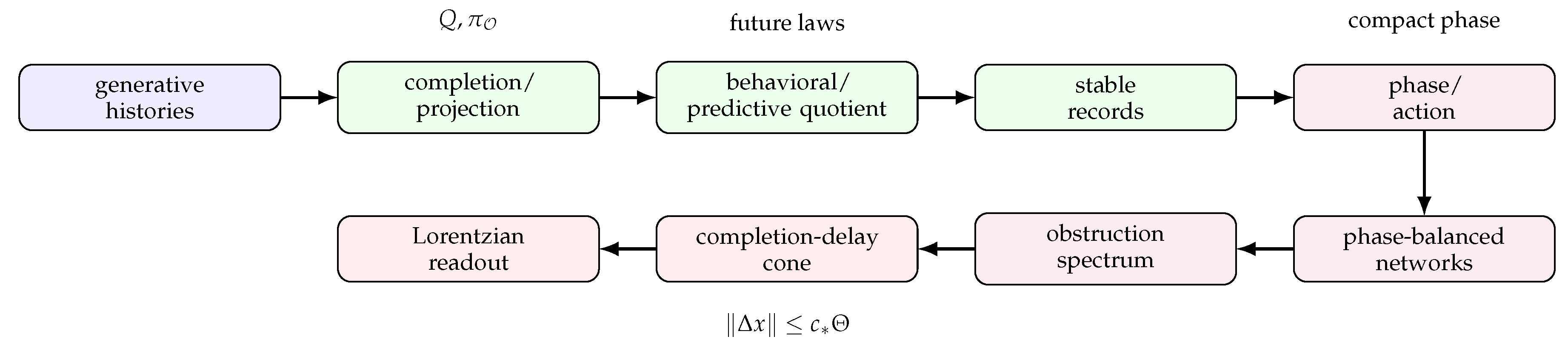
Figure 2.
Minimal working model. The main quotient branch is supplemented by the phase-selection and obstruction branches used later in the reconstruction.
Figure 2.
Minimal working model. The main quotient branch is supplemented by the phase-selection and obstruction branches used later in the reconstruction.
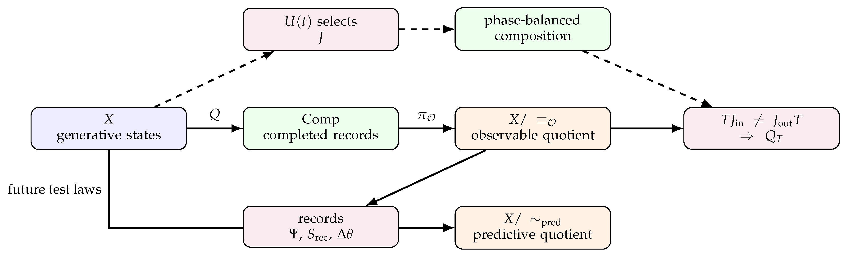
Figure 3.
Dependency graph for the reconstruction framework. Inputs and theorem-level outputs are displayed as distinct nodes to make the conditional structure explicit.
Figure 3.
Dependency graph for the reconstruction framework. Inputs and theorem-level outputs are displayed as distinct nodes to make the conditional structure explicit.
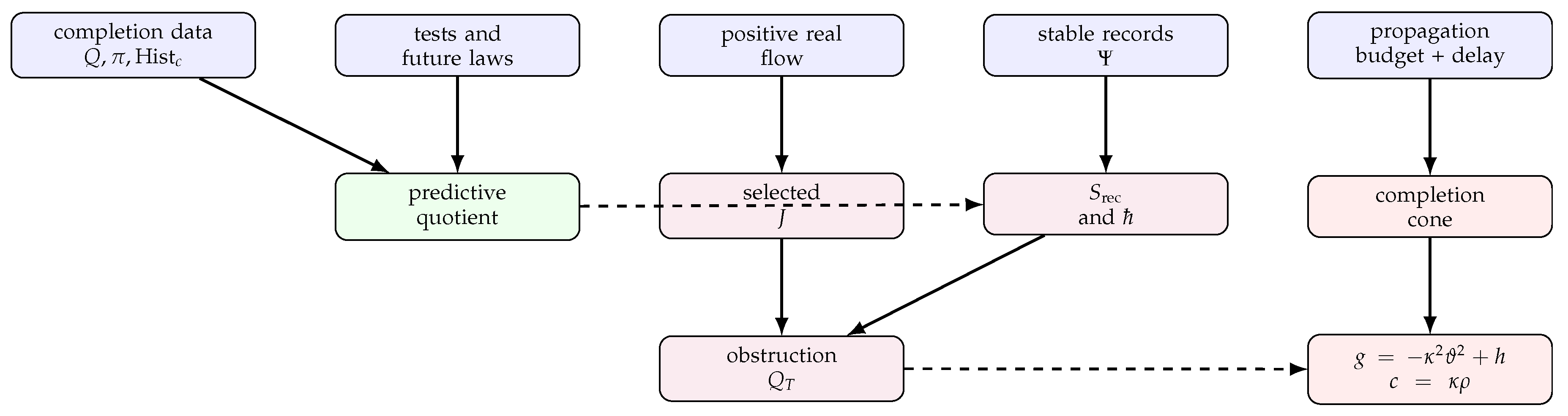
Figure 4.
Variational predictive selection. The selected presentation is the least complex robust statistic preserving the relevant future laws and supporting stable records.
Figure 4.
Variational predictive selection. The selected presentation is the least complex robust statistic preserving the relevant future laws and supporting stable records.
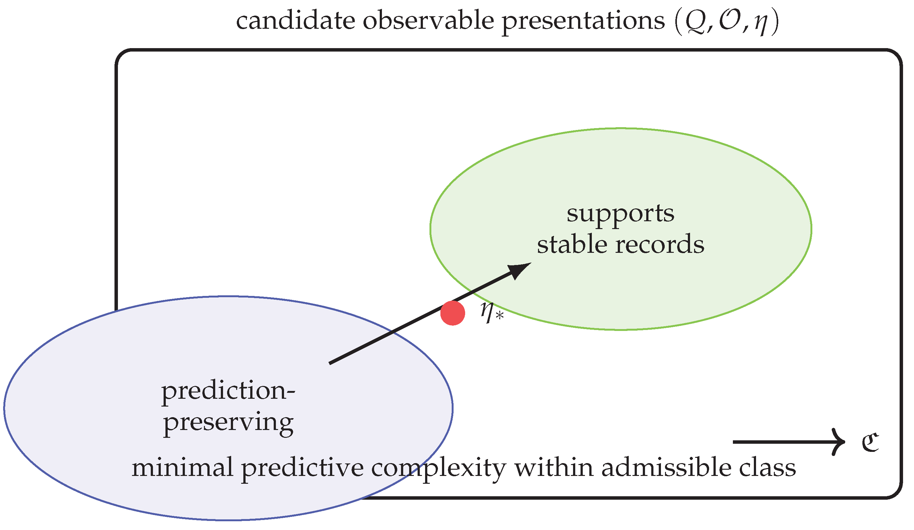
Figure 5.
Predictive compression and the record scalar. The endpoint defect is represented by loss of predictive information under observational compression.
Figure 5.
Predictive compression and the record scalar. The endpoint defect is represented by loss of predictive information under observational compression.

Figure 6.
Algebraic-geometric envelope. Algebraic families of histories, completion, and quotienting are organized by the corresponding descent and moduli structures.
Figure 6.
Algebraic-geometric envelope. Algebraic families of histories, completion, and quotienting are organized by the corresponding descent and moduli structures.
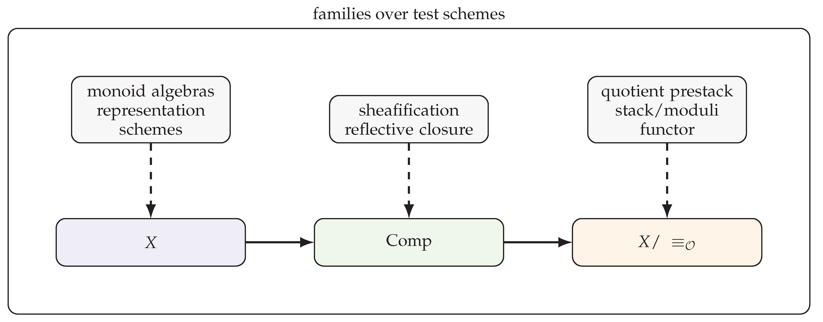
Figure 7.
Descent obstruction for phase-sign quotients. A coarse quotient can lose the transition data retained by the quotient stack.
Figure 7.
Descent obstruction for phase-sign quotients. A coarse quotient can lose the transition data retained by the quotient stack.
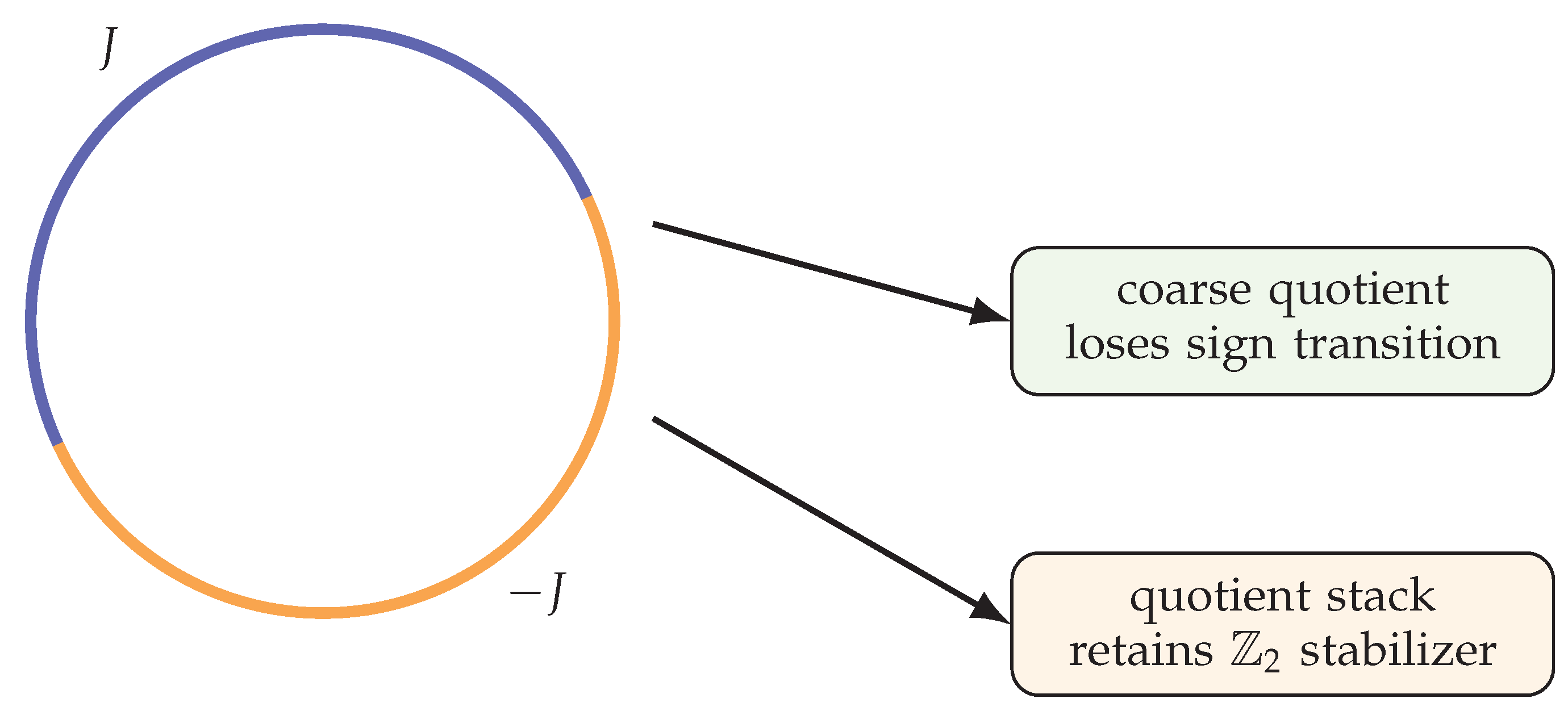
Figure 8.
Real-commutant phase parameter space. Candidate imaginary units are intrinsic to the real representation, and positive energy selects the stationary phase operator.
Figure 8.
Real-commutant phase parameter space. Candidate imaginary units are intrinsic to the real representation, and positive energy selects the stationary phase operator.

Figure 9.
Phase-balanced network composition. The quotient relation supplies the shared phase standard needed for complex tensor composition.
Figure 9.
Phase-balanced network composition. The quotient relation supplies the shared phase standard needed for complex tensor composition.

Figure 10.
Endpoint stable records and compact phase. Endpoint cocycle additivity fixes the record action correction, and compact phase additivity fixes the phase-action character.
Figure 10.
Endpoint stable records and compact phase. Endpoint cocycle additivity fixes the record action correction, and compact phase additivity fixes the phase-action character.
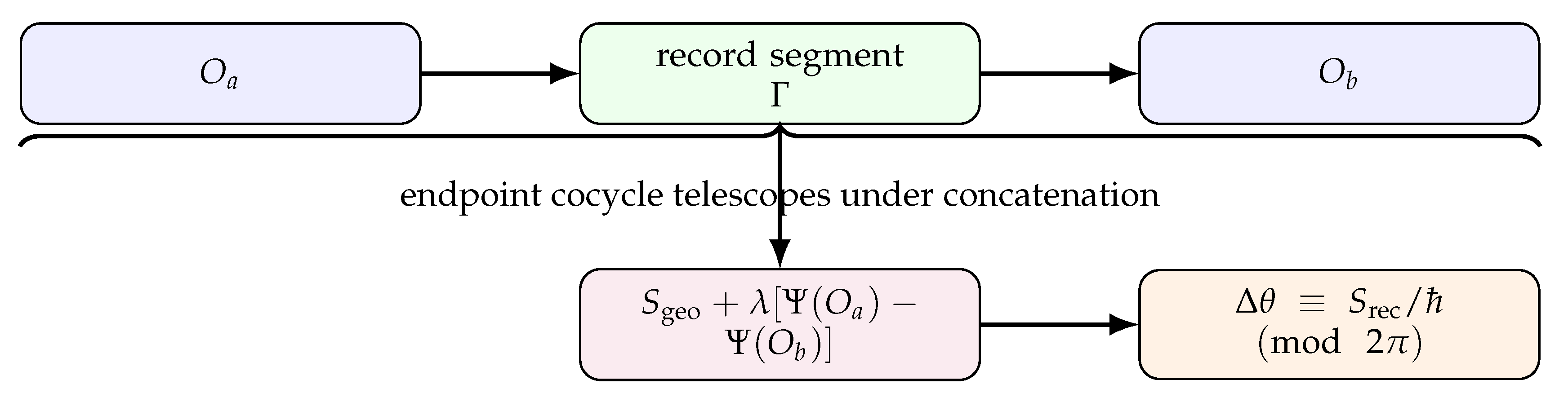
Figure 11.
Predictive-record interferometer. Branch-dependent predictive laws determine a residual phase through their relative predictive-information defect.
Figure 11.
Predictive-record interferometer. Branch-dependent predictive laws determine a residual phase through their relative predictive-information defect.
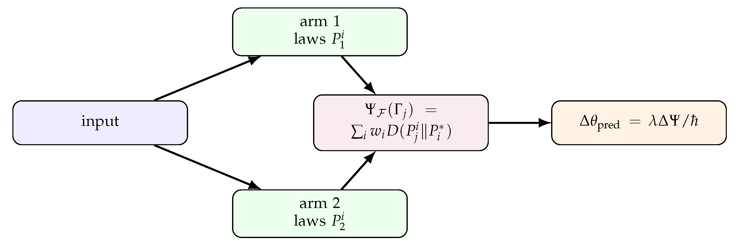
Figure 12.
Obstruction-spectrum diagram. The antilinear component produces the basis-free positive occupation operator .
Figure 12.
Obstruction-spectrum diagram. The antilinear component produces the basis-free positive occupation operator .
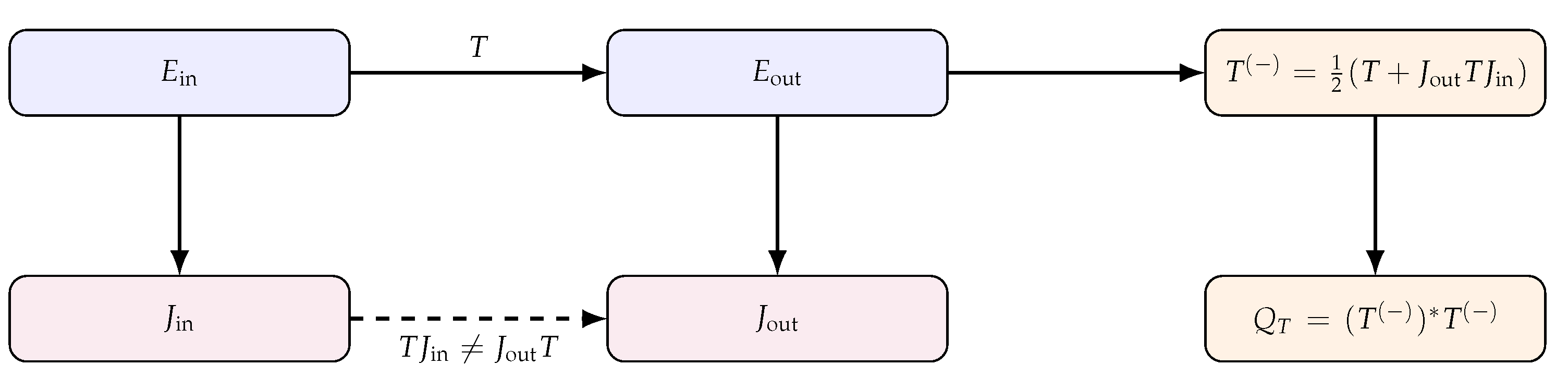
Figure 13.
Bridge between obstruction spectra and network phase balancing. Both structures test transport or sharing of selected phase operators.
Figure 13.
Bridge between obstruction spectra and network phase balancing. Both structures test transport or sharing of selected phase operators.
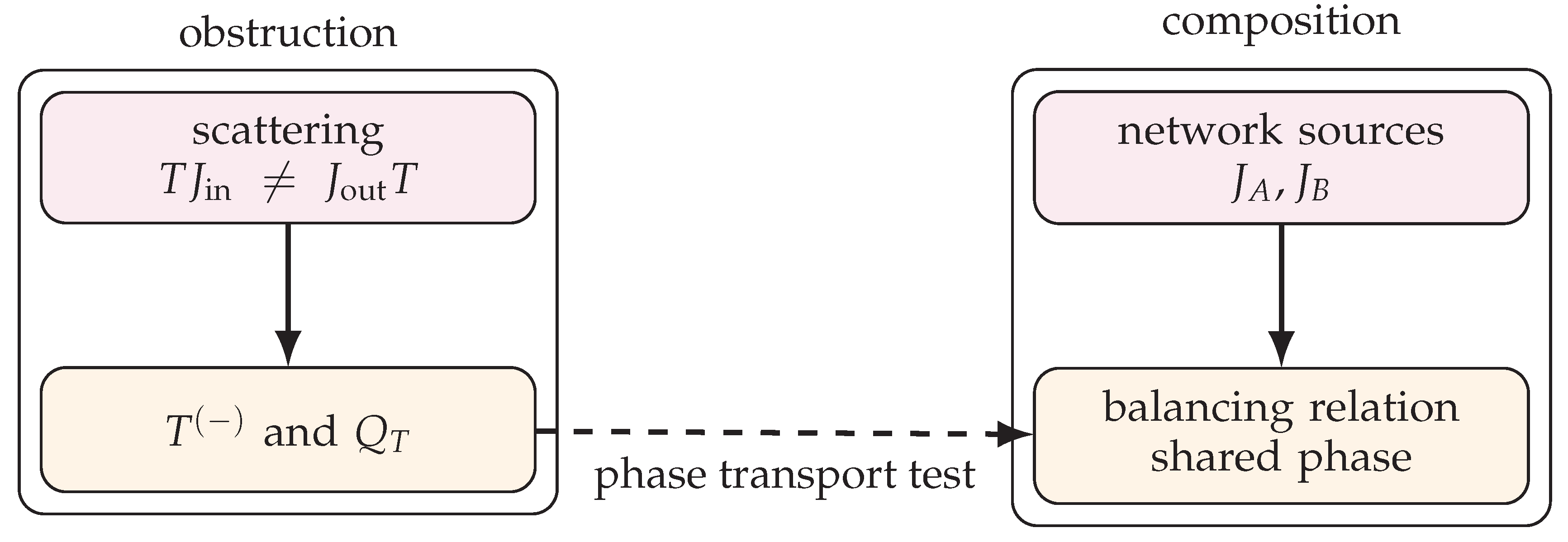
Figure 14.
Obstruction-spectrum data. The invariant observable is the spectral data of , not coordinate entries of a Bogoliubov matrix.
Figure 14.
Obstruction-spectrum data. The invariant observable is the spectral data of , not coordinate entries of a Bogoliubov matrix.
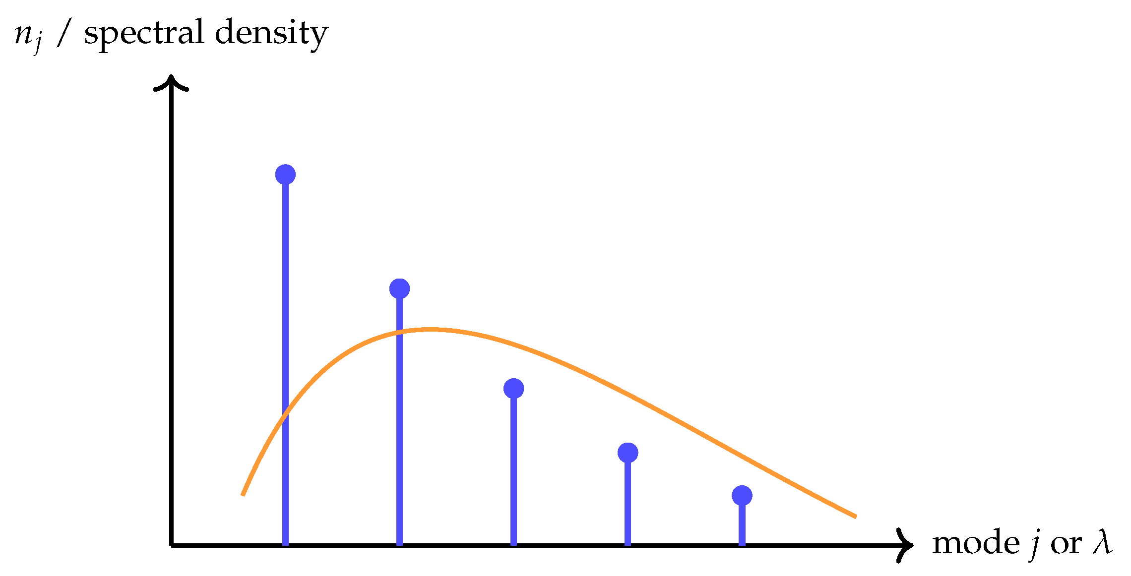
Figure 15.
Geometry-layer reconstruction. Lorentzian readout passes through a finite completion cone, a smooth connection-geometry lift, and stabilized continuum reconstruction.
Figure 15.
Geometry-layer reconstruction. Lorentzian readout passes through a finite completion cone, a smooth connection-geometry lift, and stabilized continuum reconstruction.

Figure 16.
The finite observer-level cone. The cone is a consequence of completed propagation budget, not a primitive spacetime metric.
Figure 16.
The finite observer-level cone. The cone is a consequence of completed propagation budget, not a primitive spacetime metric.
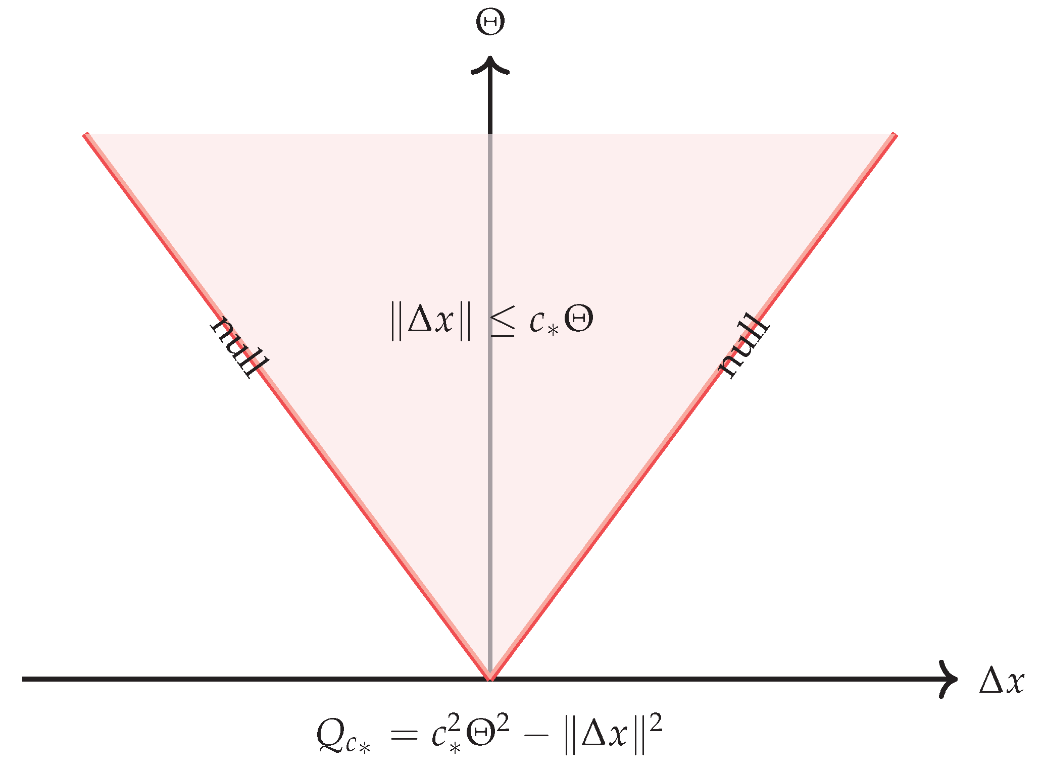

Table 1.
Input-output dependency table for the reconstruction framework. The table is deliberately local: each output depends on its own input layer, so weakening an input weakens or removes the associated conclusion.
Table 1.
Input-output dependency table for the reconstruction framework. The table is deliberately local: each output depends on its own input layer, so weakening an input weakens or removes the associated conclusion.
| Reconstructed output | Required input layer | What fails if removed |
|---|---|---|
| Observable irreversibility | Completion/projection quotient compatible with histories | No descended observable arrow or memory mechanism. |
| Minimal predictive observable state | Stochastic completed-future test laws and predictive equivalence | Observable quotient may retain redundant distinctions or lose future statistics. |
| Variationally selected test family | Complexity, sufficiency, and stable-record constraints on candidate observables | The test family remains an external input rather than a selected presentation. |
| Selected imaginary unit J | Real orthogonal flow plus positive time orientation | Complex structure remains a free parameter. |
| Phase-balanced network composition | Independently selected local J operators plus a balancing relation or shared phase reference | Isolated real simulations may work, but source-independent network correlations lack a common phase standard. |
| Stable action | Endpoint-stable record closure and scalar | Action corrections may be arbitrary or history-dependent. |
| Phase law | Compact phase additivity and action equivalence | No forced linear phase-action character. |
| Obstruction spectrum | Positivity-selected in/out phases and real transition T | No basis-free particle-creation invariant. |
| Lorentzian cone readout | Local propagation budget plus completion-delay law | No observer-level speed bound or null cone. |
| Smooth Lorentzian metric | Completion cone plus smooth inner-time connection, spatial readout, and calibration | No connection-induced metric or theorem. |
| Manifoldlike spacetime reconstruction | Stabilized order and volume in a manifoldlike sector | No effective continuum spacetime geometry is reconstructed. |
Table 2.
Status of reconstructed, calibrated, imported, and open structures.
| Structure | How we use it |
|---|---|
| Complex structure J | Reconstructed from positive real dynamics on the nonzero-frequency sector. |
| Real-commutant parameter space | Derived from the real representation and canonical conjugation. |
| Predictive quotient | Reconstructed, in stochastic operational models, as the minimal sufficient state for future completed test statistics. |
| Test family and predictive laws | Inputs in the proved quotient theorems; proposed to be selected by a variational predictive-sufficiency principle rather than left arbitrary. |
| Shared imaginary unit in composites | Reconstructed as the phase-balancing quotient identifying selected local J operators; operationally tested by source-independent network composition. |
| Endpoint scalar | Model input in the general endpoint theorem; in predictive realizations it may be selected as a monotone predictive-information functional. |
| Action correction | Forced inside the endpoint stable-record closure class. |
| ℏ as action-per-radian constant | Reconstructed as a protocol-level conversion slope after compact phase calibration. |
| Numerical SI value of ℏ | Imported by metrological calibration of the action unit. |
| Born rule | Not reconstructed here. |
| Interacting quantum field theory | Not derived here; only linear/quasifree and controlled obstruction layers are treated. |
| Finite Lorentzian cone | Reconstructed from a local propagation budget and a completion-delay law. |
| Connection-induced limiting-speed metric | Reconstructed in smooth regimes from the completion cone by representing delay with a connection one-form and spatial readout with a horizontal metric; the speed is . |
| Continuum Lorentzian geometry | Reconstructed only in stabilized manifoldlike order-volume sectors. |
| Gravitational field equations | Not derived here. |
Disclaimer/Publisher’s Note: The statements, opinions and data contained in all publications are solely those of the individual author(s) and contributor(s) and not of MDPI and/or the editor(s). MDPI and/or the editor(s) disclaim responsibility for any injury to people or property resulting from any ideas, methods, instructions or products referred to in the content. |
© 2026 by the authors. Licensee MDPI, Basel, Switzerland. This article is an open access article distributed under the terms and conditions of the Creative Commons Attribution (CC BY) license (http://creativecommons.org/licenses/by/4.0/).
Copyright: This open access article is published under a Creative Commons CC BY 4.0 license, which permit the free download, distribution, and reuse, provided that the author and preprint are cited in any reuse.


