

Submitted:
19 May 2026
Posted:
21 May 2026
You are already at the latest version
Abstract
Bose’s original derivation of the photon occupation statistics employs a counting procedure in which identical quanta are distributed among distinct phase-space cells. In this paper, we present an alternative interpretive derivation of the Bose–Einstein distribution for photons, in which the suppression of permutations arises from causal ordering constraints associated with relativistic propagation and detector geometry, complementing the standard formulation based on particle identity. The derivation is mathematically equivalent to the standard approach and leaves all quantum predictions unchanged. The analysis is confined to the source–detector rest frame relevant to the measurement. A thought experiment demonstrates that introducing dispersive media preserves both the causal-ordering mechanism and its mathematical equivalence to Bose's indistinguishability approach. This work offers a complementary perspective to the conventional formulism by clarifying the interpretive foundations of photon statistics.
Keywords:
photonics
; Bose-Einstein statistics
; photon counting
; Planck radiation law
; blackbody radiation
; photonic toroidal vortex
1. Introduction
The standard derivation of the Bose-Einstein distribution, introduced by Bose in 1924 [1], treats photons as indistinguishable in principle when unobserved. This assumption—that identical quantum particles lack individual identity even conceptually—has become a cornerstone of quantum statistical mechanics. However, Bose's original derivation contains an interpretive asymmetry: while photons are treated as indistinguishable due to lack of observation, the cells of abstract six-dimensional phase space among which they are distributed are treated as distinguishable despite being entirely unobservable mathematical constructs.
This paper makes this asymmetry explicit and offers a resolution by treating both photons and cells as distinguishable in principle, with both located in real rather than abstract space. We explore whether an alternative, fully equivalent counting mechanism can be constructed without invoking ontological indistinguishability. The present work demonstrates that the Bose-Einstein distribution can be derived from distinguishable photons subject to a crucial physical constraint: photons emitted in sequence maintain that sequence during transit. This constraint arises from causality—photons traveling at the same speed c cannot pass one another. We show that this sequence preservation produces the same occupation-number counting as Bose's indistinguishability assumption, but with a visualizable physical mechanism.
Our approach employs a geometric photon model from recent work on photonic toroidal vortices [2], which assists in the statistical argument when a dispersive medium is introduced. The model is tested using the hemispherical blackbody (HSBB) geometry—an experimentally validated design used in infrared radiometer calibration [3]—with cell-tubes running from emission points to a detector at the hemisphere's focus.
Section 2 reviews the historical development of blackbody radiation theory, highlighting unresolved conceptual issues in Planck's and Einstein's approaches. Bose's counting method is examined in Section 3 where the interpretive asymmetry is identified. Section 4 presents our cell-tube framework, deriving the photon-to-cell relationship especially in dispersive media, and recovering Planck's law. Section 5 discusses the relationship to Bose's method, and broader implications for quantum indistinguishability.
2. Brief History
Following an earlier attempt by Wien [4],1 in 1900, Planck [6] succeeded in obtaining a formula for the energy density of a blackbody in the frequency interval that was in good agreement with the data of Rubens and Kurlbaum [7].2 Two years earlier, Planck had found a relationship between the energy density and the average energy per oscillator based on the classical theory of oscillating electrons [8]:3
However, he now had found the correct formula for the average energy per oscillator [6]
where is the Boltzmann constant and is the temperature. Unfortunately, Planck’s attempted theoretical justification contained several crucial errors as follows.
(1) As Jeans remarked, no population was given from which a probability could be calculated [9].
(2) Ehrenfest objected that oscillators of a particular frequency could only exchange energy among themselves [10], p.166. This meant that an initial unstable distribution had no mechanism by which it could be redistributed into the universal function, Eqs. (1) and (2).4
(3) Einstein pointed out that while Eq. (1) had been derived on the basis of Maxwell’s theory of electrodynamics using continuous spatial functions, the energy in Eq. (2) had been obtained using a sum over a set of discrete energy values [12].5
Planck never managed to overcome these difficulties.
In 1916, Einstein obtained Planck’s radiation law, Eqs. (1) and (2), by equating emission and absorption rates of radiation [13,14]. In doing so, he considered three radiation processes for a particular frequency : (a) spontaneous emission in the absence of incident radiation, (b) induced emission from incident radiation, and (c) radiation absorption. The method assumes that the radiation is not a classical spherical wave but has a directed momentum with magnitude where (). A molecule is taken to be isotropic so that the and coefficients are independent of direction. However, no mechanism is given for the emission and absorption of radiation, and no explanation is given as to what determines whether an irradiated molecule participates in (b) or (c). Instead, Einstein relegated these events to chance remarking that “the assumed statistical law corresponds to a radioactive reaction” [14].6
3. The Bose Counting Method
In 1924, Satyendra Nath Bose derived Planck’s law using a novel counting procedure that amounted to treating any two photons with identical intrinsic properties as indistinguishable [1].7 There are two parts to his derivation.
(1) For the th frequency interval , is the number of cells in a six-dimensional phase space with volume .8 Following Einstein, the assumption that the momentum of a light quantum is a vector with magnitude is adopted, but Bose also introduces an abstract six–dimensional phase space in which the photon state is described at any instant by a point . Since each photon has two polarization senses, the number of cells available in the th frequency interval is given by
Although unobservable, the cells are still regarded as distinguishable in principle.
(2) A calculation for the most probable distribution among the cells in this interval is based on a novel method of counting photons. What Bose means by ‘distribution’ is that for each frequency interval , there is a count of the numbers of cells containing 0, 1, 2, … photons, with these numbers assigned to the variables . The number of available cells is determined by Eq. (3). There are also constraints on the total number of available quanta, and the constant total energy so that
So for each frequency interval governed by , Bose considers the number of ways that the set of values can be assigned subject to these constraints. The aim is to obtain as a function of and , and obtain the set of that is most frequent for a probability calculation.
In Bose’s method, since the photons are being considered prior to observation, they cannot be distinguished even in principle. However, the cells among which the photons are to be distributed are located in a mathematical space and cannot be observed at all. So they should also be treated as indistinguishable. Nevertheless, in order to represent the cells in a definite sequence, Bose was forced to treat them as distinguishable.9 This represents an interpretive asymmetry worth examining. It can further be noted that the notion of cells in a mathematical space fails to serve as a physical explanation. How are the cells arranged in the real space of the container? This is the question that will be addressed here, and to answer it, we shall use cells and photons that are both distinguishable in principle.
4. The Cell-Tube Sequence
4.1. The Cells
Here, we treat the number of possible photon locations or cells in a container. Let a photon consist of a rotating string on a notional tube, see Figure 1 [2], footnote 8.10 This is denoted as Sp-1 rotation.
Our cell will consist of this cylindrical tube and since then the volume of this notional tube is given by
Assuming that the two circular polarisation senses can occupy the same space, the number of cells per unit volume is then
The Hemispherical Blackbody (HSBB) is designed to calibrate measurements of longwave downward radiation in infrared radiometers that are used in climate research. In Figure 2, the HSBB has an Infrared Integrating Space (IRIS) located at ABCD just below the aperture at the focus to measure the light intensity. This geometrical design has been tested and has been found to have a commendable “low correlation between the total effective emissivity and the observation angle” [3, Figure 2a].11
Let us allow photons to impinge on the entry surface S of an IRIS, see Figure 3. Then Eq. (6) is too restricted as it only applies to cells that are orientated normal to this surface.12 For incidence at an angle to the normal, the area of the end of the cell tube is distributed over a larger elliptical area, diluting the effect of a photon in that tube on a target electron in the IRIS. The area of an ellipse is where is the length of the semi-major axis and the length of the semi-minor axis. When a tube is inclined at an angle to the detector normal , one axis becomes elongated by a factor and the other remains the same. So the area of the ellipse is and for the effective number of cells per unit volume in the frequency interval at angle , Eq. (6) becomes modified to
4.2. Photon Emissions
Photons directed at ABCD are to be emitted from an internal surface element X with area — shaded in Figure 2. In Figure 3 the angles are not equivalent as far as the effect of cells on the detector is concerned so a weighting must be applied. The fraction of the total number of cells available from the internal surface area of the hemisphere is
From Eq. (7), the effective number of cells per unit volume available in the intervals , , and is then
Integration will then produce the average effective number of cells.
4.3. Photon Energy
Since the photon momentum approaches the photodiode at an angle then the components of the momentum and energy normal to the photodiode surface are given by
With Eqs (9) and (10) established, all that remains is to find a relationship between the number of photons and the number of available cells in the intervals , , and so that the average energy per unit volume can be obtained.
4.4. The Statistical Count
By way of example, let us run a linear cell-tube from the element on the container interior to an element on ABCD, see Figure 2.
The cell-tube is to carry photons — represented as arbitrarily small bounded volumes for brevity — that have been emitted from area element to the target area element . Now, an essential feature of this stream of photons is that since they all have the same speed their order of emission remains invariant during transit. The emission sequence referred to here is defined relative to the rest frame of the emitting surface and the detector, which are assumed to be stationary with respect to one another (as in the HSBB calibration geometry). In this frame, photons propagate at the same speed c along each cell-tube and cannot overtake one another, so the emission order is invariant during transit. No claim is made that this ordering is Lorentz-invariant between arbitrary inertial frames; the statistical counting is performed entirely within the source-detector rest frame relevant to the measurement.
By way of example, in Figure 4 let us imagine an arbitrarily small time interval in which there are 13 photons in a five-cell tube and the number of cells containing photons is , respectively.13 Our interest is in the number of ways this distribution can occur. To calculate this, we keep the cell partitions fixed and move the photons around the cells subject to the conditions without altering their order. This is illustrated in Figure 5 and with the number of possible arrangements is
First, the number of permutations of the cells is found. Then for each group — the group of cells containing r photons — the number of permutations of the cells in that group is reduced to one by dividing by This ensures that the emission order of the cells in that group is retained.
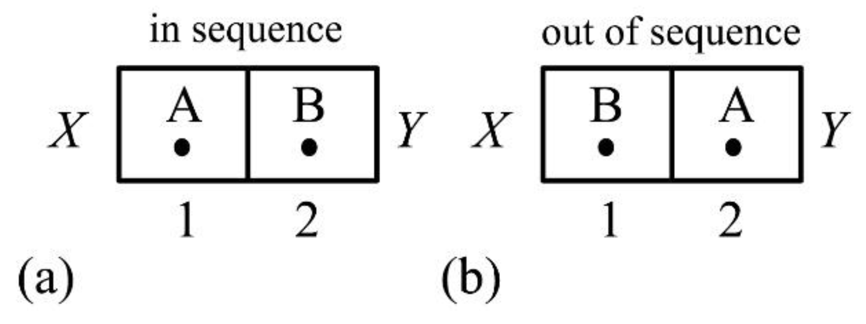
In Figure 6a, two photons have been emitted from X towards Y, first B then A. These are to be distributed among two distinguishable cells 1 and 2 under the condition that each cell is to have only one photon. If the emission order is to be maintained, there is only one way of achieving this as shown in Figure 6a. In Figure 6b, the reverse order A then B is not possible, but this is not because we are assuming that AB cannot be distinguished either observationally or in thought from the order BA. It is because once the emission order has been established towards Y, no photon can pass another, and so the sequence cannot be changed. So, in considering how the photons might be distributed among the available cells, we vary the spacing between photons so that they can change cells into while maintaining the same sequence, see Figure 5.
It turns out that the number of possible arrangements of the photons amongst the cells in a cell-tube for each distribution is calculated from
where is the number of cells with zero photons, is the number with one photon, and so on. The distribution with the maximum number of possible arrangements, subject to the total photon number and energy constraints, is the most probable distribution for the cell-tube in the given frequency interval.
Consider a cell-tube with the radius of the hemisphere in Figure 2. Let us define as the number of cells containing photons in the th frequency interval for the th distribution so that the total number of available cells in the cell-tube is given by
and the total number of quanta assigned to a cell-tube to be distributed amongst these cells is
From Eq. (4), the constraint on the constant total energy in a cell-tube in the th frequency interval is
From Eq. (12), the total number of distributions is the sum over all distributions and is a constant
The probability of the th distribution in the interval then becomes
The entropy of this distribution is to follow Boltzmann’s law
We now aim to maximise the entropy (18) with respect to the by varying the distribution subject to the constraints Eqs (13) and (14). Applying the variation to Eqs (17) and (18) gives
having used Stirling’s approximation with and as constants. Varying Eqs (13) and (15) accordingly produces
and
noting that the zeros arise from the constancy of and as the distribution is varied. The use of undetermined multipliers and permits Eqs (19), (20), and (21) to be combined as
Since this holds for any variation , each term in parentheses vanishes to yield the most probable distribution as
where is constant. Using Eq. (13)
Returning to Eq. (14) and making use of Eq. (23) we also have
where can be determined.
This solves the problem of the relationship between the total number of photons and the total number of cells in a cell-tube in the frequency interval . We now assume that all cell-tubes in the frequency interval contain the same ratio of photons to cells expressed in Eq. (25). In this way, the analysis can be scaled up to the entire volume of the hemisphere in Figure 2.
However, as far as the absorption of photon energy is concerned, not all cell-tubes are equivalent. If the angle of incidence is , the area of the cell-tube on the detector increases with so that the number of photons per unit area diminishes as — see Eq. (9). The component of momentum of the photon taken normal to the photodiode will also decrease with — see Eq. (10). So, from Eqs. (9) and (25), the average number of photons per unit volume in the intervals , , and is given by
Consideration of Eq. (10) gives the average energy per unit volume in these intervals as
The following integration then yields the Planck law for the average energy per unit volume in as
4.5. Relationship to Bose's Method
Both our distinguishable-photon approach and Bose's indistinguishable-photon approach arrive at the same occupation-number counting formula, Eq. (12). This mathematical equivalence reflects a deeper structural similarity between the two methods that merits careful examination.
Bose's reduction mechanism: In Bose's framework, photons with identical intrinsic properties are treated as fundamentally indistinguishable. This means that any two arrangements of photons among cells that result in the same occupation numbers { ...} are considered the same microstate, not distinct microstates. For example, "photon A in cell 1, photon B in cell 2" is identical to "photon B in cell 1, photon A in cell 2" if we cannot distinguish A from B. The division by the denominator of Eq. (12) eliminates this overcounting.
Our reduction mechanism: In our framework, photons are distinguishable by their position in the emission sequence. However, the emission sequence must remain invariant during transit because photons traveling at speed c cannot pass one another (Figure 6). When we redistribute photons among cells while preserving emission order, many permutations that would be accessible to classical distinguishable particles become forbidden.
The crucial observation: Both methods arrive at Eq. (12) through different physical mechanisms:
- Bose: Quantum indistinguishability forbids distinguishing permutations
- Proposed method: Causal ordering constraints associated with relativistic propagation forbid certain permutations
Mathematically, the constraint "preserve emission sequence" acts identically to "treat particles as indistinguishable." This raises the question of whether some statistical consequences commonly associated with quantum indistinguishability also be reproduced by causal ordering constraints in geometric arrangements?
Interpretive implications: From an instrumentalist perspective, both derivations are empirically successful —they reproduce Planck's law with equal accuracy. From a realist perspective, however, the approaches differ fundamentally.
Limitations of our approach: We emphasize four important caveats:
- Limited scope: Our derivation applies to photons in blackbody equilibrium. Extension to other bosonic systems (e.g., Bose-Einstein condensates of atoms) would require additional geometric arguments.
- No claim of primacy: We do not assert that our interpretation replaces or improves upon Bose's standard formulation. Both are consistent with observation. We claim only that the distinguishable-photon framework provides an alternative conceptual foundation that some may find more intuitive and that may offer complementary pedagogical value.
- Mathematical equivalence: The numerical predictions are identical. Our contribution is interpretive and pedagogical rather than empirical.
- Geometrical constraint: The present analysis has only been shown to apply to a hemispherical container. More general containment needs to be investigated.
4.6. A Thought Experiment
Consider a cell-tube (Figure 4) with spatially varying refractive index along its length from emission point X to detector element Y. Specifically, let the central region have decreased refractive index, causing photons to accelerate relative to adjacent regions. This thought experiment clarifies what remains invariant under such transformations and why the counting method is robust.
The fundamental invariant is the emission sequence A→B→C→...→M. When photons enter the acceleration region, they speed up by factor s (velocity ratio), increasing the spatial separation between consecutive photons by the same factor. Upon exiting the region, they decelerate back to speed c. Throughout this process, no photon overtakes another — the sequence is preserved.
What changes is the physical distribution of photons in space. As photons accelerate and spread apart, the effective cell boundaries stretch with them. In the central acceleration region, cells become physically larger (stretched), containing the same photons but now distributed over greater spatial extent. At the trailing boundary where photons decelerate, cells compress back to their original size.
The physical basis for this cell-size variation follows directly from the photon's wavelength change in the dispersive medium. From Eq. (5), each cell has volume , where is the photon wavelength. When a photon accelerates in the lower refractive index region, its wavelength increases proportionally (). The cell volume therefore increases as s³. This is not an arbitrary stretching — the cell size must change because it is defined by the photon's own wavelength. A faster photon with longer wavelength naturally occupies a larger cell volume. When the photon decelerates upon exiting the dispersive region, its wavelength decreases back to , and the cell volume returns to its original size. The photons move with their assigned cells, maintaining their cell memberships while their spatial coordinates change. Since the combinatorial count in Eq. (12) depends only on the occupation numbers {p₀, p₁, p₂, ...}, not on the physical coordinates of cell boundaries or their sizes, the statistical counting is completely unaffected. Three quantities remain invariant:
- The emission sequence A→B→C→...→M (photons cannot overtake)
- The occupation numbers {p₀, p₁, p₂, ...} (same photons in same cells)
- The combinatorial count in Eq. (12) and therefore the probability distribution
This thought experiment demonstrates that the causal-ordering mechanism is robust under transformations that preserve sequence. Both our distinguishable-photon framework and Bose's indistinguishable-photon framework predict the same result: only the occupation distribution at the detector matters, not the propagation path or the nature of the dispersive medium.
The absence of a distinguishing test between these interpretations reflects a deep structural similarity: causal ordering constraints in relativistic propagation produce the same statistical consequences as quantum indistinguishability. The fact that cell-size variations (driven by wavelength changes in dispersive media) leave the statistical counting unchanged demonstrates the robustness of this correspondence. Whether this geometric-quantum equivalence is merely mathematical or points to deeper physical connections between photon structure and quantum statistics remains an open question worthy of further theoretical investigation.
5. Conclusions
A novel derivation of the Bose-Einstein distribution has been presented in which both photons and the cells they occupy are treated as distinguishable in principle. This approach offers a resolution to an asymmetry in Bose's original 1924 method, where unobserved photons were treated as indistinguishable while unobservable cells in abstract six-dimensional phase space were treated as distinguishable. The key features are as follows.
- Geometric realization: Abstract phase-space cells are replaced with physical cell-tubes in real space, running linearly from emission points on a hemispherical blackbody interior to a detector at its focus. This geometry has been experimentally validated for infrared radiometry [3].
- Physical mechanism: The occupation-number counting formula Eq. (12) emerges from a classical constraint — emission sequence preservation — rather than from quantum indistinguishability. Photons traveling at the same speed in the same dispersive-medium locality cannot pass one another, forbidding certain permutations and naturally producing Bose-Einstein statistics.
- Mathematical equivalence: Our distinguishable-photon framework reproduces Planck's radiation law exactly, Eq. (28). The numerical predictions are identical to Bose's method, but the physical interpretation differs fundamentally.
- Connection to PTV framework: The photon structure (Figure 1) is borrowed from the photonic toroidal vortex model [2], lending weight to the analysis of dispersive media behaviour, and demonstrating consistency across that research program. However, the statistical argument stands independently—any photon representation with finite volume Eq. (5) and two polarization states yields the same result.
This work raises a foundational question: To what extent might some phenomena commonly attributed to quantum indistinguishability also be reproduced by geometric ordering constraints? The emission-sequence preservation in our model acts identically to indistinguishability in Bose's model, producing the same occupation-number statistics through different physical mechanisms. This suggests that geometric and quantum-mechanical descriptions may offer complementary perspectives on the same physical phenomena. Our derivation applies to photons in blackbody equilibrium. Extension to other bosonic systems (e.g., atomic Bose-Einstein condensates, superfluid helium) would require additional arguments and remains an open question.
Conflicts of Interest
On behalf of all authors, the corresponding author states that there is no conflict of interest.
| 1 | Wien had calculated intensities that were lower than those given by the data of Lummer and Pringsheim in the 0.7–6 long wavelength region for various cavity temperatures [5]. |
| 2 | Heinrich Rubens visited Planck on 7 October 1900 to communicate their results. Planck guessed the correct form of the radiation law the same evening. |
| 3 | He presented the paper to the Berlin Academy of Sciences on 7 July 1898. |
| 4 | This flaw remained in a later theory that Planck presented to the 1911 Solvay Congress in Brussels. At this meeting he suggested that while the absorption of energy by oscillators is a continuous process, energy emissions occur in integral multiples of . He also introduced the concept of a zero point energy h [11]. |
| 5 | In the same paper, Einstein pointed out that when is large then monochromatic radiation behaves “as if it consisted of mutually independent energy quanta of magnitude [h]”. |
| 6 | “Though he would be able to bring a ready derivation of Planck’s theorem using his coefficients, Einstein would never be able to extract a proper physical link” [15], p.11. |
| 7 | Shortly after translating Bose’s paper into German, Einstein applied Bose’s counting procedure to a monatomic ideal gas in order to account for the low temperature deviation from the classical equation of state [16]. |
| 8 | Sachur had already proposed dividing a quantum-theoretical phase space into cells with volume for molecules [17]. |
| 9 | An arrangement with two photons in cell A and one in cell B is a distinct microstate from an arrangement with one photon in cell A and two in cell B. |
| 10 | |
| 11 | The observation angle was varied by moving the detector ABCD along the normal towards or away from the aperture in Figure 2. For uniformity of emissivity, the arrangement in Figure 2 was the best of the four hemispherical designs tested. The researchers also tested an alternative design in which the aperture was positioned at the opposite end of the normal to ABCD in Figure 2 with an inward-pointing conical end rather than a circular plane. When taking the possible coatings into consideration — Nextel 811-21 and Vantablack S-IR — the researchers favoured this alternative design having calculated how the diffusivity of the coatings would affect the total effective emissivity [3], Figure 2a. |
| 12 | The IRIS can be replaced by a near-infrared (NIR) spectrometer, a visible (VIS) spectrometer, and ultraviolet (UV) spectrometer, or an X-ray spectrometer depending on the wavelength region to be sampled. These typically contain a photodiode to measure the light intensity. |
| 13 | Realistically, for red light with a wavelength of 7 × 10⁻⁵ cm, there are approximately 14,000 cells per cm of cell-tube. Feieraband et al. [3] used a hemispherical radius of 10cm. |
References
- Bose, S. N., Planck’s Gesetz und Lichtquantenhypotheses, Zeitschrift für Physik 26 (1924): 178–81. [CrossRef]
- Clarke, B. R., A photonic toroidal vortex model of the hydrogen atom fine structure, Quantum Studies: Mathematics and Foundations 12, 19 (2025). [CrossRef]
- Feierabend, M., Reininger, M., Bories, J., and Adibekyan, A. Development and operation of the hemispherical blackbody (HSBB) for the calibration of infrared radiometers with a hemispherical acceptance angle, Optics Express 30, 26 (2022): 46991–47003. [CrossRef]
- Wien, W. Ueber die Energieverteilung im Emissionsspectrum eines schwarzen Körpers, Annalen der Physik 58 (1896): 662–669.
- Lummer, O., and E. Pringsheim, Die Vertheilung der Energie im Spectrum des schwarzen Körpers, Verhandlungen der Deutsche Physikalische Gesellschaft 1 (1899): 23–41.
- Planck, M. Ueber das Gesetz der Energieverteilung im Normalspectrum, Annalen der Physik 4 (1901): 553–563. [CrossRef]
- Rubens, H., and F. Kurlbaum, Anwendung der Methode der Reststrahlen zur Prufung des Strahlungsgesetzes, Annalen der Physik 4 (1901): 649–666. [CrossRef]
- Planck, M., Über irreversible Strahlungvorgänge, Annalen der Physik 1 (1900): 69–122.
- Jeans, J., A comparison between two theories of radiation, Nature 72 (1905): 293. [CrossRef]
- Kuhn, T., Black-body Theory and the Quantum Discontinuity, 1894–1912. Oxford University Press, 1978, p.166. [CrossRef]
- Planck, M., Theory of Heat Radiation. Dover, 1959.
- Einstein, A., Uber einen die Erzeugung und Verwandlung des Lictes betreffenden heuristischen Gesichtspunkt, Annalen der Physik 17 (1905): 132–148.
- Einstein, A., Strahlungsemission und absorption nach der Quantentheorie, Verhandlungen der Deutschen Physikalischen Gessellschaft 18 (1916): 318–323.
- Einstein, A., Zur Quantentheorie der Strahlung, Mitteilungen der Physikalischen Gessellschaft, Zürich 18 (1916): 47–62.
- Robitaille, P.–M., Kirchoff’s law of thermal emission: 150 years, Progress in Physics 4 (Oct 2009): 3–13.
- Einstein, A. Quantentheorie des einatomigen idealen Gases, Sitzungsberischte der Preussischen Akademie der Wissenschaften, presented to the Prussian Academy on 10 July 1924, pp.261–267.
- Sackur, O., Die Anwendung der kinetischen Theorie der Gas auf chemische Probleme, Annalen der Physik 36, 4 (1911): 958–980. [CrossRef]
- Clarke, B. R., Reinterpretation of the Grangier experiment using a multiple-triggering single-photon model, Modern Physics Letters B 37, 15 (2023), 2350042. [CrossRef]
Figure 1.
a A helical string revolving around a notional tube at speed and rake . Both the linear and azimuthal speed are . b The net of the notional tube or cell showing that .
Figure 1.
a A helical string revolving around a notional tube at speed and rake . Both the linear and azimuthal speed are . b The net of the notional tube or cell showing that .
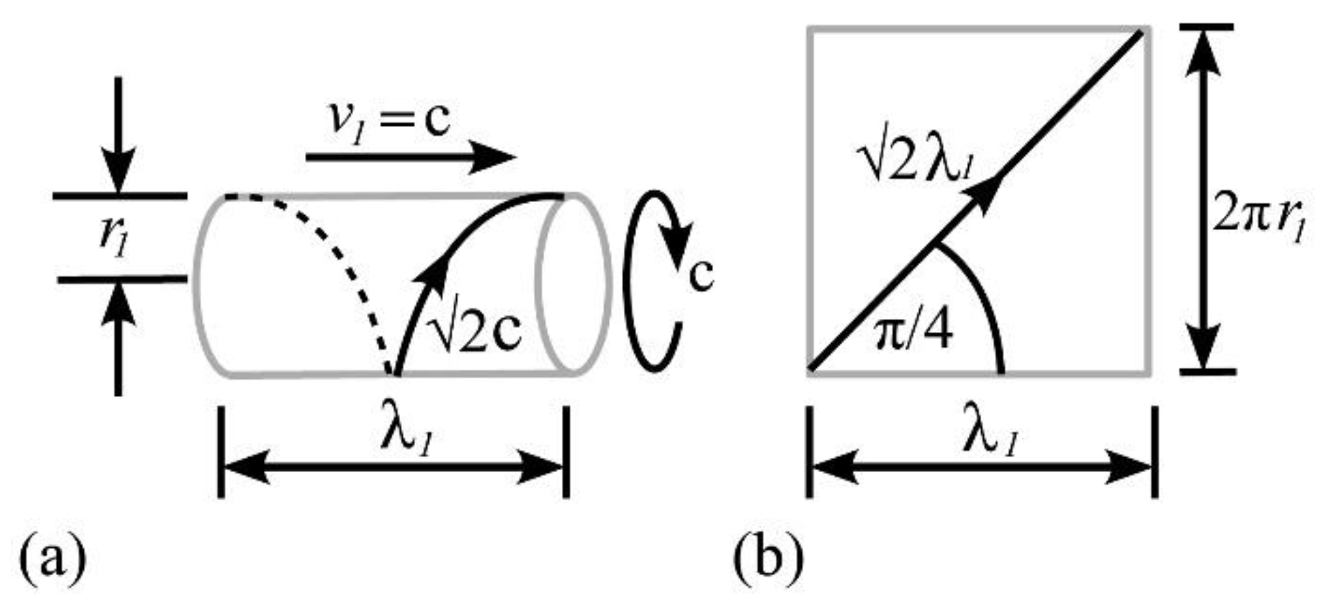
Figure 2.
A HSBB with a detector ABCD placed below the aperture at the center of the base. The shaded element has an area given by and radiates towards element .
Figure 2.
A HSBB with a detector ABCD placed below the aperture at the center of the base. The shaded element has an area given by and radiates towards element .
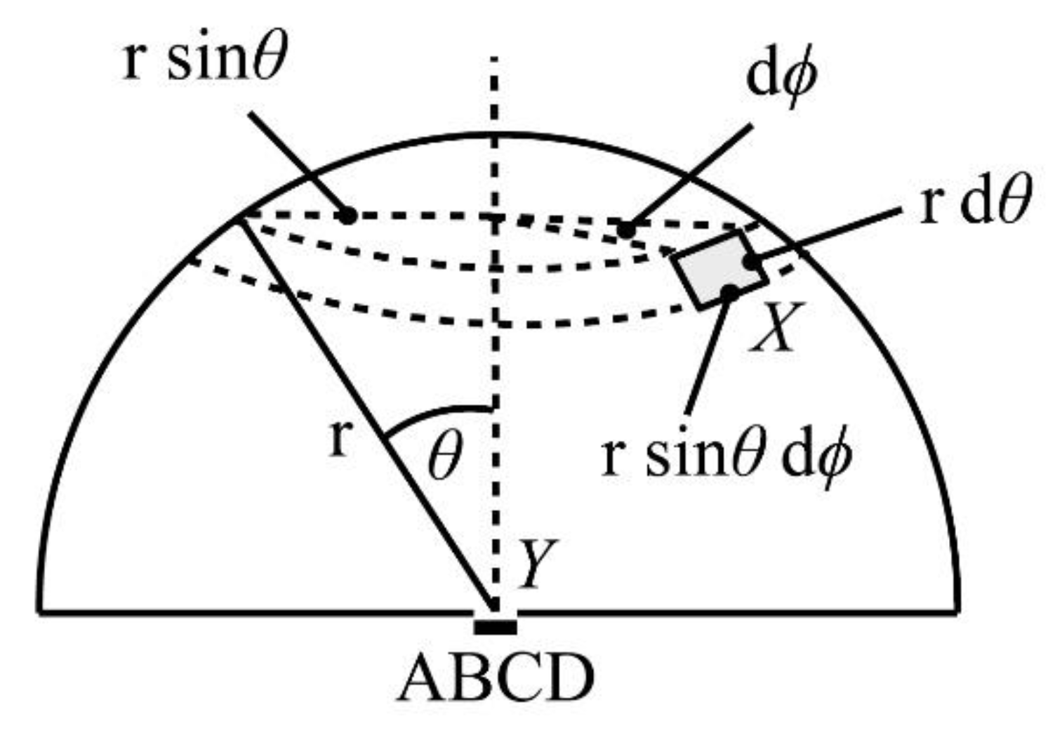
Figure 3.
a A cell tube directed towards the surface ABCD of an IRIS at angle to the normal . b Diameter PQ of the tube end becomes length on the elliptical projection of the circular tube end on ABCD. The radius perpendicular to PQ on the circular end remains on .
Figure 3.
a A cell tube directed towards the surface ABCD of an IRIS at angle to the normal . b Diameter PQ of the tube end becomes length on the elliptical projection of the circular tube end on ABCD. The radius perpendicular to PQ on the circular end remains on .
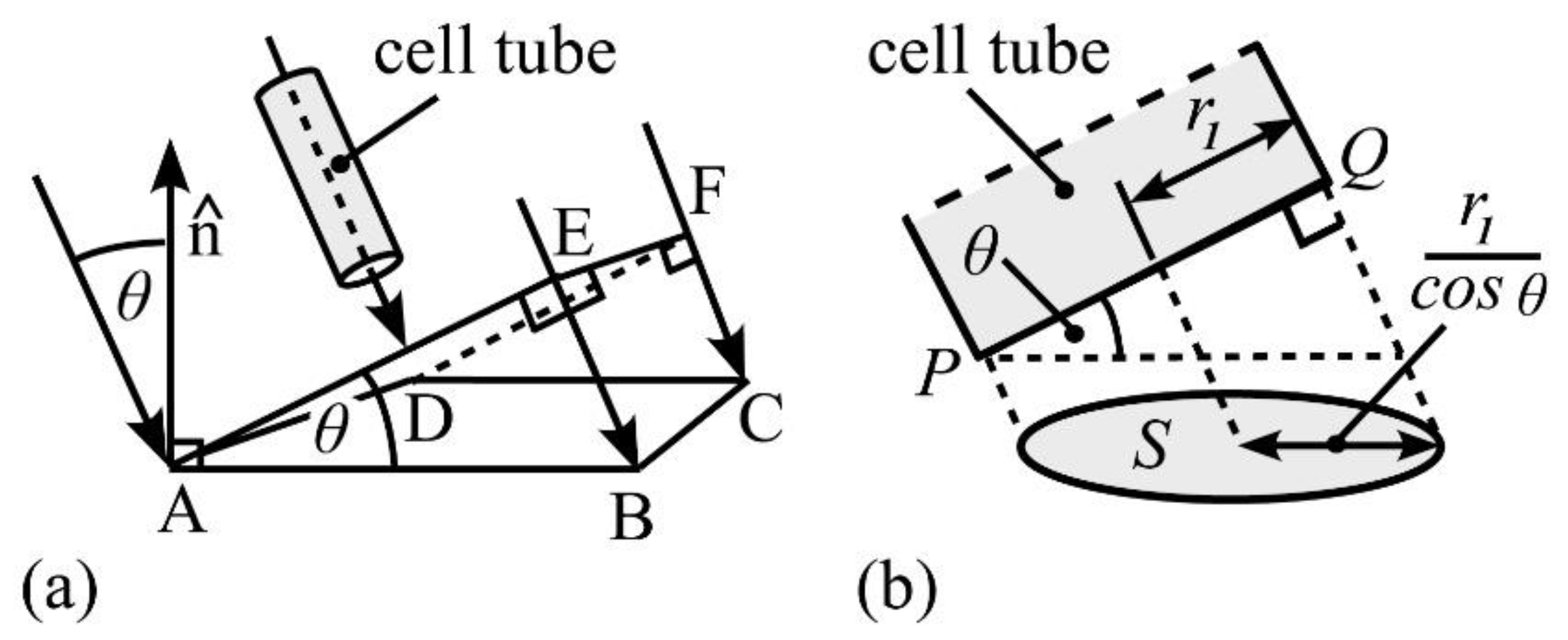
Figure 4.
An example distribution with a five-cell tube that carries a distribution of 13 photons (black dots) emitted at speed from the container area element to the area element , see Figure 2.
Figure 4.
An example distribution with a five-cell tube that carries a distribution of 13 photons (black dots) emitted at speed from the container area element to the area element , see Figure 2.
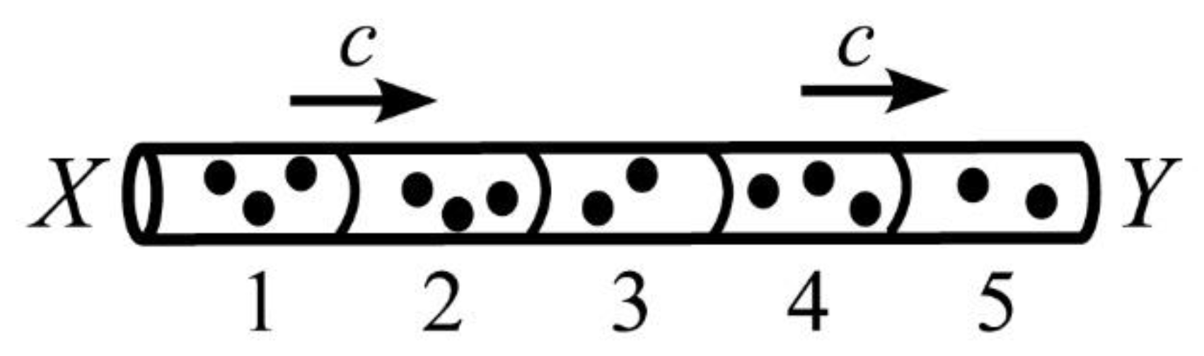
Figure 5.
The 10 distributions resulting from redistributing 13 photons among 5 cells under the condition that while retaining the photon sequence A–M.
Figure 5.
The 10 distributions resulting from redistributing 13 photons among 5 cells under the condition that while retaining the photon sequence A–M.
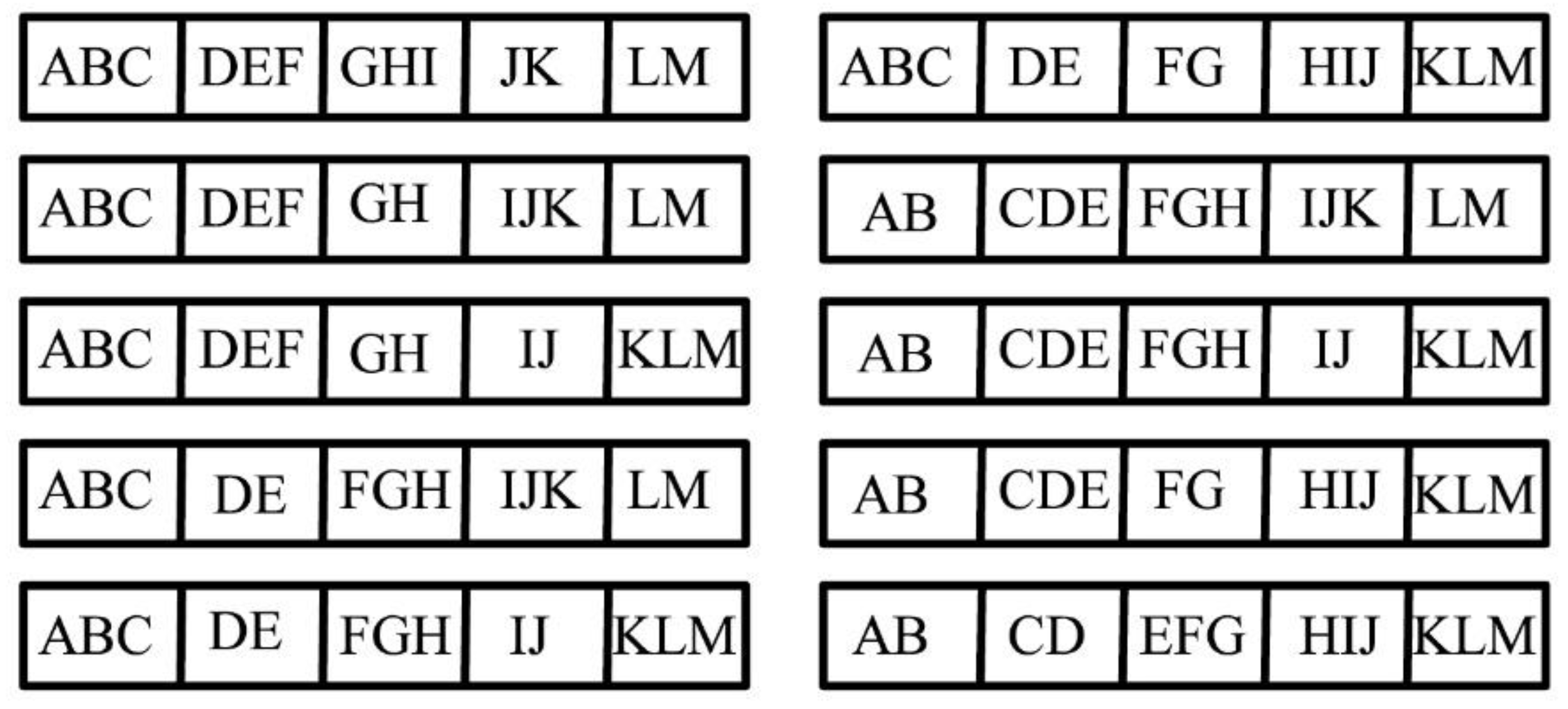
Figure 6.
Two cells 1 and 2 and two photons A and B with only one allowed in each cell. a The photons travel from X to Y in their order of emission, B then A, reading from right to left. b The order cannot be reversed to A then B as shown because photon A cannot overtake B.
Figure 6.
Two cells 1 and 2 and two photons A and B with only one allowed in each cell. a The photons travel from X to Y in their order of emission, B then A, reading from right to left. b The order cannot be reversed to A then B as shown because photon A cannot overtake B.
Disclaimer/Publisher’s Note: The statements, opinions and data contained in all publications are solely those of the individual author(s) and contributor(s) and not of MDPI and/or the editor(s). MDPI and/or the editor(s) disclaim responsibility for any injury to people or property resulting from any ideas, methods, instructions or products referred to in the content. |
© 2026 by the author. Licensee MDPI, Basel, Switzerland. This article is an open access article distributed under the terms and conditions of the Creative Commons Attribution (CC BY) license.
Copyright: This open access article is published under a Creative Commons CC BY 4.0 license, which permit the free download, distribution, and reuse, provided that the author and preprint are cited in any reuse.


