

Submitted:
20 May 2026
Posted:
21 May 2026
You are already at the latest version
Abstract
The transition to net-zero energy systems involves substantial uncertainty in exogenous conditions such as policy, fuel prices, and technology deployment. Conventional energy system optimization models, formulated as forward problems, excel at identifying a single least-cost solution but provide limited insight into the diverse configurations feasible within an acceptable cost range. This study proposes a hierarchical inverse-analysis framework integrating a genetic algorithm (GA) and linear programming (LP). The upper-level GA explores a broad space of exogenous conditions, including policy conditions, fuel prices, end-use electrification rates, and CO2 capture rates, while the lower-level LP rigorously optimizes operations for each candidate. The framework applies explainable AI (SHAP) to identify dominant cost-determining factors and their interactions, and employs k-means clustering to compress the high-dimensional feasible solution space into representative scenarios. As an illustrative demonstration, the framework is applied to a hypothetical 2050 net-zero case for the Kanto region. The results confirm diverse solution generation, identification of dominant factors, and extraction of five representative scenarios, enabling systematic distinction between common and variable elements characterizing net-zero pathways. The proposed framework extends energy system modeling beyond single-optimum solutions toward interpretable decision-support analytics for long-term net-zero planning under deep uncertainty.
Keywords:
energy system optimization
; Inverse analysis
; genetic algorithm
; explainable AI
; clustering
1. Introduction
1.1. Background
Japan has established the goal of achieving carbon neutrality (CN) by 2050 as a national policy and, in June 2021, released the Green Growth Strategy Through Achieving Carbon Neutrality in 2050 [1]. As reflected in the strategy's coverage of 14 industrial sectors and eight policy tools, the technologies and institutions required for a CN society span a wide range. As elements such as power generation, heat demand, electrification, energy storage, decarbonized fuels, and CO2 capture and storage are mutually interrelated, energy supply–demand models have become increasingly important for quantitatively examining future energy-system configurations [2].
Energy supply–demand models are broadly classified into bottom-up models, which evaluate technology choices under a given demand level, and top-down models, which describe energy supply and demand in relation to economic activity [3]. Bottom-up energy system optimization models, in particular, are well suited to evaluating technology selection, installed capacity, and operational states from a cost-minimization perspective under specified demand and technological conditions. In Japan, representative models such as DNE21+ [3,4] and IEEJ-NE [5] have been developed and applied to long-term energy supply–demand analyses toward 2050. In recent years, scenario analysis has become more robust through soft-linking approaches that enable the mutual use of results across multiple models [6,7].
However, most conventional energy system optimization models are formulated as forward problems, in which a cost-minimal solution is computed under a given set of assumptions. Consequently, analytical outputs are often limited to a single optimal solution or a small number of cases predefined by the analyst. Although such analyses are useful for long-term investment planning and policy assessment, they are not necessarily sufficient for identifying practical alternatives under substantial uncertainty in the underlying assumptions.
This limitation is particularly important for micro-level decision-makers, such as firms and regional actors. Investments toward a CN society are made under medium- to long-term uncertainty and are constrained by factors such as grid connection and permitting; therefore, cost-minimal choices are not always realized in practice. Actual investment decisions are influenced by social acceptability, institutional change, fuel-price volatility, equipment deployment feasibility, and technological progress, many of which are difficult to represent explicitly within a model. From a decision-support perspective, energy supply–demand models are therefore required not only to present a single optimal solution, but also to identify multiple alternative system configurations achievable within a given cost range, together with the conditions under which each becomes viable. Such a capability enables responses to questions such as "How should one respond if a particular business environment emerges?” and “What options exist for implementing a given strategy?" This task can be formulated as an inverse problem, in which causes are inferred from outcomes and feasible solution sets are explored. Conventional models, however, remain limited in their ability to address such inverse problems flexibly and efficiently. The present study seeks to provide a methodological foundation in this direction.
1.2. Related Work and Research Gap
The motivation for this study—the need to identify multiple alternative system configurations achievable within a given cost range, together with the conditions under which each becomes viable, rather than presenting only a single optimal solution—is related to two strands of prior research. The first is research on Modeling to Generate Alternatives (MGA), which generates diverse alternatives within a near-optimal region instead of presenting only a single optimal solution [8]. The second is research on hierarchical design optimization, in which the upper level determines equipment configuration and capacity while the lower level optimizes operation under that configuration. The following reviews both strands and clarifies the position of the present study.
MGA was proposed as a framework for generating alternatives that achieve comparably favorable objective values while differing substantially from one another. The classical work by Brill et al. introduced the idea of intentionally generating multiple alternatives to accommodate factors that are difficult to incorporate into a model, rather than presenting only the optimal solution [8]. DeCarolis extended this concept to the energy domain, arguing that systematic exploration of the near-optimal region through MGA can broaden perspectives on possible energy futures [9]. Price and Keppo applied MGA to TIAM-UCL, a global energy–environment–economy model, and showed that technologically distinct transition pathways exist within the near-optimal region [10]. Neumann and Brown showed that, even within very small cost differences, numerous technologically distinct near-optimal solutions exist for a European power system with a high share of renewables [11]. Lau et al. reviewed and compared MGA methods, showing that the choice of vector-selection method affects exploration breadth, efficiency in identifying extreme solutions, and computational performance [12].
These studies have been highly influential in establishing the importance of considering diverse alternatives within the near-optimal region rather than relying on a single optimal solution. However, most existing studies first solve for the optimum, then impose slack constraints around it, and sequentially explore the model's internal capacity or design variables. This reflects a methodological limitation: when MGA includes operational variables such as annual generation in the alternative-generation objective, weights unrelated to actual operating costs are introduced, causing dispatch to deviate from the principle of least-cost operation and undermining economic dispatch [12]. Consequently, exploration tends to remain confined to capacity-related variables. Additionally, few studies have simultaneously explored a broad assumption space that includes exogenous and institutional conditions such as policy settings, fuel prices, demand-side electrification rates, and CO2 capture rates. Moreover, even when MGA produces many near-optimal solutions, the results are typically represented as a high-dimensional point cloud that is not directly useful for decision support. Practical application therefore requires an additional step that organizes numerous solutions into representative design archetypes and presents the conditions under which each archetype emerges in an interpretable form m.
In hierarchical design optimization, methods have been proposed in which equipment configuration and capacity are determined at the upper level, while operation is optimized at the lower level under the given configuration, with the aim of optimally designing energy supply systems. Yokoyama et al. introduced a mixed-integer linear programming (MILP) branch-and-bound method that exploits the hierarchical relationship between design and operational variables to efficiently solve optimal design problems for energy supply systems [13]. This approach explicitly handles design variables while embedding lower-level operational optimization, thereby enabling rigorous treatment of large-scale design problems. Wakui et al. [14] proposed a two-stage optimization approach combining an artificial immune system (AIS) with MILP, separating the upper-level structural design problem from the lower-level operational problem and efficiently obtaining diverse design candidates for large-scale energy supply networks. Yokoyama et al. further extended the hierarchical MILP approach to derive K-best solutions, providing a method for systematically enumerating multiple design alternatives following the optimal solution [15].
These studies demonstrate that hierarchical frameworks separating upper-level structural design from lower-level operational optimization are effective for energy supply systems. Their objectives, however, differ. The basic hierarchical MILP method was developed primarily to derive a single optimal solution efficiently, whereas the K-best extension and the AIS–MILP approach explicitly aim to obtain multiple design candidates [14,15]. Even so, the primary targets of exploration in these studies are internal design variables such as equipment configuration and capacity, and the systems considered are formulated as design problems for energy supply systems, distributed energy systems, cogeneration systems, or energy supply networks. Although some studies consider seasonal and time-resolved multi-period operation, they differ from research targeting a regional energy supply–demand system over the medium-to-long term toward 2050 and primarily seeking to explore assumption combinations feasible under long-term socioeconomic and institutional uncertainty. In contrast, the present study employs a heuristic genetic algorithm (GA) [16,17] for upper-level exploration to flexibly search a broad assumption space, including institutional conditions, price conditions, demand-side electrification rates, and CO2 capture rates, while LP optimizes operation for each individual at the lower level.
The novelty of this study lies in incorporating a GA into the upper level of an established hierarchical design-optimization framework to emphasize broader exploration and the generation of diverse solutions, while extending the analytical scope to a medium-to-long-term regional energy supply–demand system. Additionally, prior studies have rarely developed frameworks that organize multiple solutions into interpretable representative scenarios incorporating sensitivity structures and viability conditions. In contrast, the present study connects diverse-solution generation with explainable AI and clustering in downstream analysis, thereby transforming the solution set into a form suitable for decision support.
In recent years, explainable AI techniques have been widely adopted to improve the interpretability of complex models. Shapley additive explanations (SHAPs), proposed by Lundberg and Lee [18], provides a consistent framework for evaluating each feature's contribution to a predicted value, enabling not only feature-importance analysis but also identification of contribution direction and feature interactions. However, few studies have integrated explainable AI with diverse-solution generation in energy systems or addressed, in a unified manner, both characterization of sensitivity structures in the assumption space and extraction of representative scenarios.
In summary, three gaps remain in the existing literature. First, MGA research has demonstrated the importance of diversity within the near-optimal region, but its exploration has focused mainly on design variables, with limited systematic exploration of the exogenous assumption space, including institutional and price conditions. Second, hierarchical design optimization studies have provided effective computational frameworks for upper-level design and lower-level operation, but they have largely concentrated on equipment configuration and have not been sufficiently extended to exploration of exogenous assumption sets. Third, frameworks that organize numerous feasible solutions and their realization conditions into interpretable representative scenarios remain limited.
1.3. Objective
The objective of this study is to develop a hierarchical energy supply–demand model integrating combinatorial optimization and linear programming to generate diverse assumption sets under which a specified state can be realized, and to propose a new analytical framework that enables sensitivity analysis and extraction of interpretable representative scenarios from the generated assumption sets. Specifically, the GA explores an assumption space encompassing institutional conditions, price conditions, demand-side electrification rates, and CO2 capture rates, while LP performs operational optimization for each individual, thereby generating a large number of total cost–assumption data points. Machine learning and explainable AI are then used to identify the principal drivers of total cost and their interactions, while clustering of the feasible solution set yields a small number of comparable representative scenarios, or archetypes. The primary aim of this study is not to forecast or evaluate the future of a specific region under realistic conditions, but to propose a methodological framework and demonstrate its effectiveness under hypothetical conditions.
1.4. Contributions
This study offers four methodological contributions. First, it shares MGA's motivation of moving beyond a single optimal solution to address diverse feasible solutions, while extending the scope of exploration to the exogenous assumption space. In existing MGA and hierarchical design optimization studies, the principal exploration targets have largely been limited to equipment capacity and design variables. In contrast, this study presents a methodology that systematically explores combinations of exogenous assumptions—including institutional conditions, price conditions, demand-side electrification rates, and CO2 capture rates—by adopting a heuristic GA at the upper level and combining it with LP at the lower level.
Second, the study reconciles the flexibility of alternative generation with the rigor of operational optimization through hierarchical separation. The upper-level GA stochastically explores the assumption space, while the lower-level LP minimizes operating cost subject to supply–demand constraints for each individual. This hierarchical structure circumvents the dispatch-breakdown problem that arises in MGA when operational variables are incorporated into the objective function, while still enabling the generation of diverse alternatives.
Third, the study introduces a sensitivity-analysis approach that uses the diverse solution set as training data. By inputting numerous assumption–total cost data points into explainable AI, the study establishes a methodology for extracting the sensitivity structure of a high-dimensional assumption space. Whereas conventional one-at-a-time sensitivity analyses require iterative optimization with sequential parameter changes, the proposed approach uses generated diverse solutions as learning samples and efficiently identifies principal factors and their interactions through SHAP.
Fourth, the study establishes a downstream step that compresses the diverse solution set into representative scenarios through clustering. This enables the framework not only to generate diverse solutions but also to use their distributional structure to organize representative assumption combinations and present them as comparable scenarios suitable for decision support.
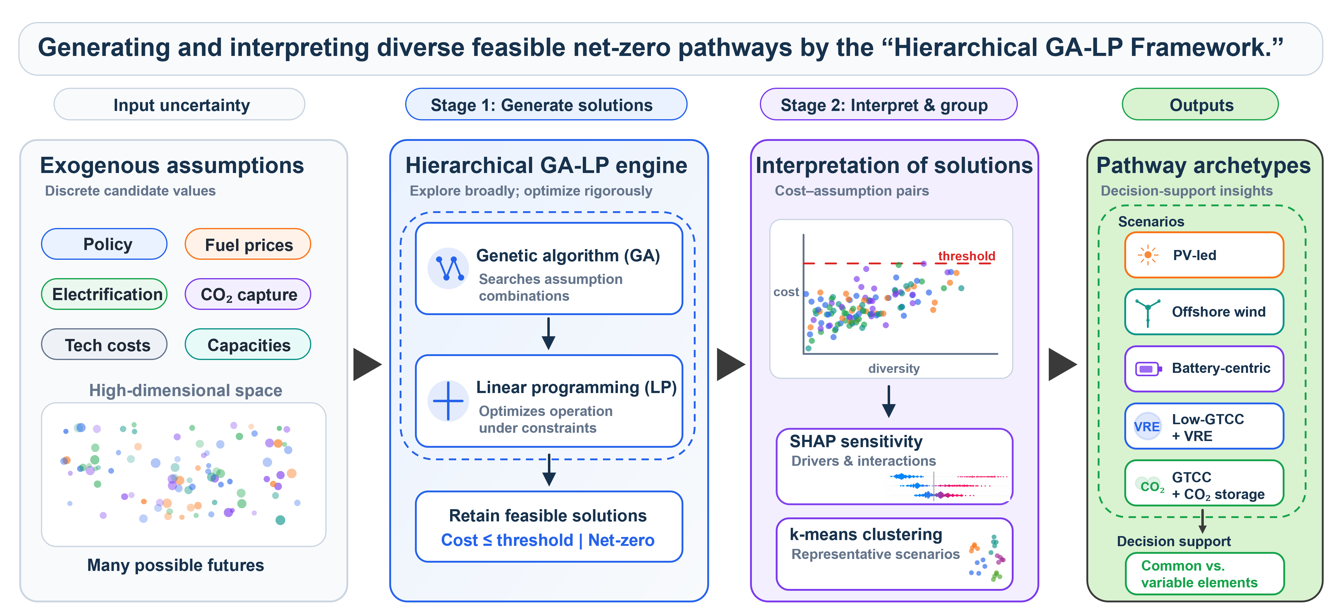
Figure 1 provides an overview of the proposed framework. The framework comprises two stages. In the first stage, the integrated GA–LP model generates a set of diverse feasible solutions. In the second stage, sensitivity analysis and representative-scenario extraction are performed. Beyond simply generating diverse solutions, the framework connects explainable AI and clustering downstream to transform the high-dimensional assumption space into interpretable insights.
The remainder of this paper is organized as follows. Section 2 describes the proposed method and demonstration setting. Section 3 presents the generation of diverse feasible solutions, sensitivity analysis, representative-scenario extraction, and identification of common and variable elements across scenarios. Section 4 discusses the methodological implications, application possibilities, limitations, and future work in light of these results.
2. Methods
This section formalizes the framework introduced conceptually in Section 1 as a concrete analytical procedure.
2.1. Overall Structure of the Proposed Framework
As shown in Figure 1, the proposed framework consists of two stages: generation of diverse feasible solutions and their interpretation and organization. In the first stage, a hierarchical inverse-analysis model integrating GA and LP generates diverse “assumption–total cost” combinations that satisfy a prescribed cost threshold. In the second stage, sensitivity analysis and clustering are applied to the resulting feasible solution set to identify the principal drivers of total cost, representative patterns under which solutions are realized, and elements that are common across scenarios as well as those that vary among them.
A defining characteristic of the proposed approach is that it adopts a stakeholder-acceptable cost level as a threshold, constructs the feasible solution set as the population of individuals satisfying that threshold, and treats the distribution of this set as the object of analysis. In other words, rather than seeking a single minimum-cost solution, the framework analyzes the structure of the feasible solution set realized under net-zero carbon conditions.
2.2. Generation of Diverse Feasible Solutions by the Hierarchical GA–LP Model
Figure 2 shows the computational flow of the integrated GA–LP approach used in this study. At the upper level, a GA explores combinations of discrete assumptions, including equipment capacities, price conditions, heat-demand electrification rates, and parameters related to CO2 capture, while at the lower level, LP determines the operational state of each individual. Through this procedure, diverse “assumption–total cost” combinations at or below the prescribed cost threshold are collected as the feasible solution set.
The methodological rationale for adopting a GA at the upper level and LP at the lower level is threefold. First, because the assumption space is structured as combinations of discrete candidate values, evolutionary computation is more suitable than gradient-based optimization. Second, the lower-level operational optimization is a cost-minimization problem with continuous variables under supply–demand balance constraints, for which LP provides rigorous and consistent evaluation. Third, the hierarchical separation between stochastic exploration at the upper level and deterministic optimization at the lower level reconciles the flexibility of alternative generation with the rigor of operational evaluation (discussed further in Section 4.1). Model details are provided in Appendix A.1.
2.2.1. Upper-Level Problem: GA-Based Exploration of the Assumption Space
In the upper-level problem, a combination of assumptions—including institutional conditions, price conditions, equipment capacities, the electrification rate of heat demand, and installation rate and performance of CO2 capture equipment—is represented as an individual i, and the GA explores the resulting high-dimensional assumption space. Each individual is encoded as a discrete chromosome composed of multiple candidate values, where each assumption is assigned one of two to five predefined discrete candidate values.
The total cost of individual i is defined as the sum of the capital expenditure and the operating expenditure computed in the lower-level problem.
Here, CAPEX i is obtained by multiplying the total capacity Capacity i,j of technology j by the unit construction cost UnitConstructionCost j, annualizing the resulting construction cost using the payback period PP j and the discount rate DR, and summing across all technologies j. OPEX I is expressed as the sum of fuel costs, operation and maintenance (O&M) costs, and other operating costs over the representative time series T.
Only individuals whose total cost is at or below the threshold are retained, constituting the feasible solution set F.
The GA is a stochastic search algorithm inspired by natural selection and inheritance, capable of efficiently exploring broad solution spaces by simultaneously maintaining a population of candidate solutions [16,17]. In the proposed approach, an initial population is first generated, after which the lower-level LP is applied to each individual to compute total cost. The resulting cost serves as the fitness value used in selection, crossover, and mutation to generate the next generation. Individuals whose total cost is at or below the threshold are retained as the feasible solution set F. Since exploration behavior can be adjusted through parameters such as crossover and mutation rates, the GA is well suited not only for local optimization but also for characterizing the distribution of an admissible solution set. In this study, the GA functions both as an optimization algorithm and as a sampling mechanism for generating diverse “assumption–total cost” data. The implementation employed the Python library DEAP [19,20]. The basic GA settings were a population size of 200, a tournament size of 5, two-point crossover, a crossover rate of 0.6, a mutation target ratio of 0.5, and 20 generations. These settings were selected to balance exploration diversity and computational cost.
2.2.2. Lower-Level Problem: LP-Based Operational Optimization
In the lower-level problem, given the equipment conditions and other assumptions provided by the upper-level GA, operating cost is minimized while satisfying the energy supply–demand balance at each time step. The objective function is annual OPEX, which includes fuel costs and O&M costs.
The electricity supply–demand balance at each time t is imposed such that electricity supplied by generation equipment and battery discharge equals net electricity demand, battery charging, electricity used for hydrogen production, and curtailment when necessary. A representative form of this balance is given by:
The principal constraints include output upper limits for generation equipment, supply–demand balance constraints, charge and discharge constraints for storage systems, and constraints related to CO2 capture and storage.
Using LP for the lower-level problem ensures tractable and consistent operational optimization for each individual. This is important because, even when a heuristic GA is used at the upper level, each candidate must be evaluated based on supply–demand feasibility and cost minimization rather than heuristic rules. The proposed GA–LP framework therefore reconciles flexibile exploration at the upper level with rigorous operational evaluation at the lower level.
2.2.3. Total Cost Evaluation, Net-Zero Condition, and Retention of Feasible Solutions
The total cost used to evaluate each individual comprises CAPEX, O&M, and fuel costs. It is evaluated by adding CAPEX—derived from the equipment conditions specified at the upper level—with the annual OPEX computed by the lower-level LP. Each candidate is therefore evaluated based on total system cost rather than operating cost alone.
The net-zero condition is defined such that CO2 emissions from thermal power generation and heat demand are captured by CO2 capture equipment, while residual emissions are captured and stored via direct air capture and storage (DACCS), ensuring that the system achieves net-zero carbon overall. A feasible solution in this study is thus defined as one that satisfies both the supply–demand balance and the net-zero constraint through emissions, capture, and storage.
The net-zero condition is conceptually expressed as:
Here, , , and denote CO2 emissions from each source; denotes source-side capture; and denotes capture via DACCS. In the implementation, CO2 emissions are computed for GTCC, BTG, and heat-demand sectors based on fuel consumption and emission factors, while source-side capture is representing according to the installation rate and performance of CO2 capture equipment.
The additional equipment requirements associated with electrification of the heat-demand sector are incorporated into CAPEX as a switching cost. This enables total cost evaluation to reflect not only supply-side technology choices but also demand-side conversion costs.
Individuals whose total cost lies at or below the prescribed threshold are retained and constitute the feasible solution set F.
2.3. Sensitivity Analysis Based on the Generated Solution Set
A key methodological feature of this section is that sensitivity analysis is not conducted as a post-hoc step independent of optimization; instead, the “assumption–total cost” data obtained through diverse solution generation are directly used as training samples. Whereas conventional one-at-a-time sensitivity analyses require repeated iterative function evaluations, the proposed approach accumulates such data as a by-product of GA-based sampling. As a result, the sensitivity structure, including high-dimensional interactions, can be extracted without additional computational burden.
In this study, a random forest is adopted as the machine learning model, with total cost as the response variable and the assumptions as explanatory variables, while SHAP [18] is used as the explainable AI method. The random forest is an ensemble learning method that applies bootstrap sampling (sampling with replacement from the dataset) to decision trees and is known for its high predictive accuracy on complex nonlinear relationships [21,22]. SHAP decomposes each feature’s contribution to the predicted value, enabling identification of feature importance, contribution direction, and feature interactions.
By constructing a machine learning model on the diverse solution set generated by the GA and applying SHAP, the sensitivity structure of total cost across the high-dimensional assumption space can be systematically interpreted. This procedure is feasible only when data obtained through broad exploration of the assumption space are available.
2.4. Representative Scenario Extraction by Clustering
The feasible solution set obtained through the GA–LP integrated approach forms a high-dimensional point cloud that is not readily interpretable or comparable for decision-makers in its raw form. Therefore, this study applies clustering to the feasible solutions below the threshold to organize numerous solutions into a small number of representative scenarios.
First, the inverse-analysis model is executed with specified constraints, exogenous values, and parameter options to obtain diverse solutions whose total cost lies at or below the threshold. Next, the principal parameters characterizing differences among solutions are extracted from each solution and used as explanatory variables for clustering. In this approach, the principal assumptions are treated as clustering features, and k-means clustering [22] is applied.
For each cluster, the cluster center and mean parameter values are calculated to identify the combination of principal parameters that characterizes that cluster. By organizing and visualizing the operational states of representative individuals within each cluster, together with the range of conditions under which the cluster is realized, both the central tendency and the variability of each scenario are captured. Integrating these results allows each cluster to be interpreted as arepresentative scenario.
The clustering step is positioned as a method for compressing the high-dimensional feasible solution set into a small number of representative scenarios suitable for decision support. This step is not merely statistical classification but an interpretive process that includes (i) identifying design archetypes, (ii) organizing the range of conditions under which each archetype is realized, and (iii) distinguishing between common and variable elements. Ensuring this interpretability is a key methodological feature distinguishing the proposed framework from existing diverse-solution generation approaches. For each cluster, the cluster center, key equipment configuration, operational characteristics, and range of realization conditions are organized together so that each cluster is presented as an interpretable scenario rather than a collection of numerical values.
In summary, the method proposed in this section integrates diverse-solution generation via GA–LP, sensitivity analysis using explainable AI, and representative-scenario extraction through clustering into a unified analytical framework.
2.5. Demonstration Setting
To demonstrate the operation of the proposed framework, a hypothetical case study is constructed for the Kanto region in 2050 under a net-zero carbon target. Figure 3 shows an overview of the energy supply–demand system used in the analysis. The target system includes generation technologies (GTCC, conventional steam power (boiler-turbine generator, BTG), photovoltaics (PV), onshore and offshore wind, nuclear, hydro, geothermal, and biomass), Li-ion batteries, pumped hydro storage (PHS), hydrogen production and methanation, CO2 capture and storage, and DACCS. Final energy consumption includes electricity and heat demand in the residential and industrial sectors.
The assumptions are defined as combinations selected from two to five discrete candidate values and include equipment capacities, unit construction costs, fuel prices, electrification rates, and the installation rate and performance of CO2 capture equipment. Based on values estimated from assumed energy-related investment in the Kanto region, the total cost threshold is temporarily set at 12 trillion JPY [23,24]. The temporal resolution is set to one hour, and a representative time series consisting of four characteristic weeks per year, exhibiting distinctive electricity demand and renewable generation profiles, is used as input.
This demonstration is a hypothetical configuration intended to illustrate the operation of the proposed framework and does not represent a forecast of the future energy system in the Kanto region. Some exogenous values and parameter settings are assumed for illustrative purposes, and analysis under realistic conditions would require separate condition settings. Detailed technical settings, data sources, and exogenous assumptions are provided in Appendix A.
Figure 3 shows a conceptual structure of the regional energy supply–demand model for the demonstration. The figure illustrates relationships among primary energy inputs, conversion technologies, storage and transport, final energy demand, and carbon management options, including CCS and DACCS.
3. Results
This section presents the results of verifying the framework introduced in Section 2 under hypothetical conditions for the Kanto region in 2050 with a net-zero target. The purpose is to illustrate that the proposed approach can integratively execute the generation of diverse feasible solutions, characterization of sensitivity structures, and extraction of representative scenarios. Accordingly, the results do not provide policy recommendations or future projections for a specific case; rather, they serve as a methodological illustration of the insights that the framework can yield.
Section 3.1 demonstrates diverse-solution generation using the GA–LP integrated approach. Section 3.2 demonstrates sensitivity analysis based on the generated data. Section 3.3 demonstrates representative-scenario extraction via clustering. Section 3.4 demonstrates identification of common and variable elements through cluster comparison.
3.1. Generation of Diverse Feasible Solutions
This section verifies that the GA–LP integrated approach proposed in Section 2.2 can generate diverse feasible solutions whose total cost lies at or below the cost threshold.
Figure 4 plots, for feasible individuals whose total cost is at or below the threshold (12 trillion JPY), the individual index on the horizontal axis and total cost (fitness value) on the vertical axis. The individual index represents the serial number assigned to feasible individuals retained during the GA search, where larger indices correspond to individuals obtained in later search stages. The total cost is defined as the sum of operating cost computed by the lower-level LP and capital and O&M expenditures. A total of 3,752 individuals were collected, of which 2,460 correspond to unique combinations of assumptions.
Figure 4 shows that individuals with total costs in the 9–12 trillion JPY range dominate in the early stage of the search. As the search progresses, the lower bound of feasible solutions gradually decreases, and low-cost individuals in the 6.5–7.0 trillion JPY range continue to be obtained. This indicates that the upper-level GA progressively identifies more cost-favorable combinations of assumptions while exploring the assumption space. At the same time, individuals in the 9–12 trillion JPY range remain present in later stages, suggesting that the proposed approach does not converge exclusively toward low-cost regions but retains feasible solutions across a wide cost range below the threshold.
To further examine solution diversity, Figure 5 shows the distribution of feasible individuals below the threshold, with a distance-based novelty score on the horizontal axis and total cost on the vertical axis. Each point represents one feasible individual. The solid line connects median total costs across twenty equal-frequency bins (vigintiles) of the novelty score, and the shaded area indicates the 10th–90th percentile range within each bin.
The novelty score measures how different an individual’s assumption combination is from others. Specifically, all explanatory variables are first normalized to the [0, 1] range using min–max normalization. The mean distance to neighboring individuals is then computed for each individual. Let denote the normalized explanatory-variable vector of individual where p is the number of explanatory variables, and the set of k nearest neighbors of . The novelty score is defined as:
where denotes the Manhattan distance. In this study, k = 10 is used and self-distances are excluded. A higher novelty score indicates a more distinctive combination of assumptions relative to nearby solutions in the feasible solution set.
Figure 5 shows that, in the low-novelty region—particularly between 0.02 and 0.05—relatively low-cost individuals with total costs of approximately 6.5–7.5 trillion JPY are densely distributed. As the novelty score increases, the representative total cost also tends to rise overall. This indicates that low-cost feasible solutions are concentrated around relatively similar combinations of assumptions, whereas accommodating more distinctive combinations requires additional cost. At the same time, a substantial number of feasible individuals with total costs at or below 12 trillion JPY are also distributed in the region with novelty scores above 0.10, indicating that increasingly diverse alternatives emerge within the feasible solution set as cost increases.
Overall, this observed novelty–cost relationship quantitatively shows that the proposed approach does not merely converge toward low-cost solutions but maintains diversity across a broad region of the assumption space, Thereby achieving diversity exploration under the cost threshold. In the next section, the principal drivers of total cost and their interactions are identified through sensitivity analysis using the generated "assumption–total cost" dataset.
3.2. Sensitivity Analysis Based on the Generated Data
This section verifies the operation of the sensitivity-analysis step proposed in Section 2.3. The objective is to confirm that the combination of random forest and SHAP can extract the principal drivers of total cost and characterize their interaction structure from the generated diverse-solution set.
A random forest model was constructed using the assumptions as explanatory variables and total cost as the response variable. Predictive performance was evaluated by four-fold cross-validation. The mean R2 across folds was 0.9002, with a standard deviation of 0.0065. Since this study does not aim to develop a highly accurate total-cost prediction model, the random-forest hyperparameters were retained at their default values. Nevertheless, the resulting performance was considered sufficient to demonstrate the operation of the proposed framework.
Figure 6 shows the top 10 assumptions with the largest contributions to total cost, ranked by mean absolute SHAP value. The horizontal axis in Figure 6(a) represents mean(|SHAP value|), that is, the average magnitude of each assumption’s contribution to total-cost prediction, while the vertical axis lists the assumptions in descending order of importance. Larger mean (|SHAP value|) indicates that the corresponding assumption has a greater influence on predicted total cost and therefore exhibits higher sensitivity.
Figure 6(a) shows that, in this demonstration, the H2 price was identified as the most influential assumption. This was followed by the construction cost of offshore wind, the construction cost of Li-ion batteries, the newly installed PV capacity, and the newly installed offshore wind capacity. The e-methane price, the CO2-capture installation rate in the high-temperature industrial heat sector, the construction cost of PV, the newly installed Li-ion battery capacity, and the residential-sector electrification rate were also included among the top 10. Although these results are obtained under hypothetical conditions, they demonstrate that the SHAP-based analysis can successfully identify the principal cost drivers.
Figure 6(b) shows the per-individual distribution of SHAP values for the same top 10 assumptions. The horizontal axis represents the SHAP value: positive values indicate that the assumption contributes to increasing total cost, while negative values indicate that it contributes to reducing total cost. The vertical axis lists the assumptions, and each point corresponds to one individual. Point color encodes the magnitude of the assumption value, with red indicating higher values and blue indicating lower values.
For the H2 price, Figure 6(b) clearly shows that higher-priced individuals tend to exhibit positive SHAP values, whereas lower-priced individuals tend to exhibit negative SHAP values. Similar trends are observed for the construction costs of offshore wind, Li-ion batteries, and PV, as well as for the e-methane price, indicating that higher values of these cost-related variables generally increase total cost. In contrast, the direction of influence is less uniform for variables related to newly installed capacity. For newly installed PV and offshore wind capacities, negative SHAP values tend to appear at lower capacities, whereas positive SHAP values are more frequently observed at higher capacities. For the CO2-capture installation rate in the high-temperature industrial heat sector and the residential-sector electrification rate, higher values tend to correspond to negative SHAP values, whereas lower values tend to correspond to positive SHAP values. The coexistence of monotonic and non-monotonic relationships indicates that the proposed step can identify diverse contribution patterns.
Figure 7 presents dependence plots showing the relationship between the value of each of four representative assumptions and its corresponding SHAP value. In each panel, the horizontal axis represents the value of the focal assumption, the vertical axis represents its SHAP value, and the color indicates the value of the assumption exhibiting the strongest interaction. Thus, Figure 7 conveys not only the standalone effect of each assumption but also conditional effects arising from interactions with other assumptions. For each parameter on the horizontal axis, the SHAP value varies across individuals even at the same parameter value, indicating that the sensitivity of each parameter's effect on total cost depends strongly on other assumptions.
Figure 7(a) shows that the H2 price exhibits negative SHAP values around 20 and shifts substantially toward positive SHAP values at approximately 60 and above. Beyond this level, changes in SHAP value with increasing H2 price become relatively small. In this region, the relationship with the color-coded CO2-capture installation rate in the high-temperature industrial heat sector is reversed relative to that observed around an H2 price of 20, suggesting that the proposed step captures changes in equipment configuration and operational modes required to satisfy the net-zero condition as the H2 price varies.
In Figure 7(b,c), the SHAP value increases stepwise with rising construction costs of offshore wind and Li-ion batteries. The point colors indicate that, for offshore wind construction cost, the positive contribution becomes larger when newly installed offshore wind capacity is high, and that, for Li-ion battery construction cost, the positive contribution increases with newly installed Li-ion battery capacity. These results show that the proposed step can capture interactions in which the influence of cost factors is amplified by deployment scale.
For newly installed PV capacity in Figure 7(d), large negative SHAP values are observed when capacity is zero, whereas SHAP values shift toward positive as capacity increases. Additionally, in the region with large PV capacity, the SHAP value tends to be lower when the color-coded H2 price is high and higher when it is low. This indicates that the proposed step can identify interactions between supply-side configurations and fuel-price conditions.
Overall, these results confirm that the SHAP analysis step consistently extracts principal drivers, identifies monotonic and non-monotonic contribution patterns, and characterizes interactions among assumptions. Conventional one-at-a-time sensitivity analyses are generally not well suited to capturing such non-linear and joint relationships among parameters. This indicates that the proposed framework, which applies explainable AI to data generated through GA-based exploration of a broad assumption space, enables comprehensive characterization of cost structure in a high-dimensional assumption space.
3.3. Representative Scenario Extraction by Clustering
This section verifies that the clustering step proposed in Section 2.4 can compress the diverse solution set into interpretable representative scenarios.
For feasible solutions below the threshold, k-means clustering was applied after standardizing the newly built capacity of high-efficiency GTCC, PV, offshore wind, and Li-ion batteries, as well as the upper limit of CO2 storage. The number of clusters was set to five. Figure 8, Figure 9, and Figure 10 show the distribution of the number of individuals per cluster, the distribution of total cost by cluster (boxplots), and the standardized mean values of the principal parameters for each cluster (heatmap), respectively.
As shown in Figure. 8, Cluster 0 contains 482 individuals, Cluster 1 contains 897, Cluster 2 contains 91, Cluster 3 contains 208, and Cluster 4 contains 782. The feasible solutions are therefore unevenly distributed and tend to concentrate in particular clusters. Figure 9 further indicates that the typical cost levels differ among clusters: Cluster 2 exhibits the highest median total cost, whereas Clusters 1 and 4 show relatively low medians. Each cluster also exhibits a certain degree of variation and should therefore be understood not as a single point but as a representative type characterized by a common structural pattern.
Figure 10 presents a heatmap of the standardized mean values of the principal parameters for each cluster. The horizontal axis represents cluster ID, and the vertical axis lists the five principal parameters used for clustering. Each cell value corresponds to the mean standardized value of the parameter for individuals belonging to the cluster: positive values denote levels above the overall mean, whereas negative values denote levels below it. Red colorindicates relatively higher parameter values, while blue color indicates relatively lower values. Based on Figure 10 and the time-series operational patterns of representative individuals (shown in Figure A1 in Appendix B), the characteristics of each cluster are summarized in Table 1.
As shown in Table 1, the clustering step organizes the large set of feasible solutions into five representative types systematically differentiated by equipment configuration, operational pattern, and the conditions under which low-cost realization is possible. These results verify that the proposed approach can extract representative scenarios suitable for decision support from a diverse solution set. Details of the cluster analysis underlying Table 1 are provided in Appendix B.
3.4. Common and Variable Elements
As an implication for future decision-support applications, this section verifies that comparisons among the representative scenarios extracted through clustering can be used to identify common and variable elements.
Comparison of the five representative clusters shown in Table 1 reveals both tendencies shared across all clusters and tendencies that differ among them. Common tendencies include deployment of renewables at or above a certain scale, provision of flexibility to accommodate supply–demand variability, and the importance of H2 price as a condition for low-cost realization. By contrast, variable tendencies include the dominant renewable technology (PV or offshore wind), the principal source of flexibility (battery storage, GTCC, or a combination of both), the extent of CO2 storage utilization, and the combinations of conditions that become bottlenecks for low-cost realization.
The ability to distinguishthese common and variable elements verifies one of the key methodological contributions of the proposed approach. By linking diverse-solution generation with representative-scenario extraction, the framework compresses numerous feasible solutions into an interpretable structure that distinguishes “what is common” from “what varies.” In future decision-support applications using real-world data, this information-compression capability could serve as a basis for distinguishing robust investment targets from domains requiring flexible domain-making.
It should be noted, however, that the specific common and variable elements observed in this demonstration were obtained under hypothetical conditions and should not be interpreted as universal claims applicable under realistic conditions. A more detailed discussion of these common and variable elements is provided in Appendix C.
4. Discussion
4.1. Methodological Implications
This section discusses the methodological significance of the analytical framework presented in Section 1 by contrasting it with research on MGA, hierarchical design optimization, one-at-a-time sensitivity analysis, and conventional uses of clustering.
Relative to conventional MGA, the present study shares the underlying motivation of valuing diverse alternatives within the near-optimal region but differs in both its exploration target and computational structure. As discussed in Section 1.2, existing MGA studies typically first solve for the optimal solution, then impose slack constraints around it, and explore alternatives mainly with respect to capacity or design variables [8,9,10,11]. By contrast, the present study extends upper-level exploration beyond equipment capacity to include exogenous assumptions related to institutional conditions, price conditions, and demand-side conversion, such as the H2 price, e-methane price, heat-demand electrification rate, and CO2-capture installation rate. The diversity obtained in this study is therefore expressed not only as differences in equipment design but also as diversity in the assumption space, representing an extension beyond conventional MGA. As shown by the cost distribution and novelty–cost relationship in Section 3.1, the proposed approach generates not only solutions near the minimum-cost solution but also structurally distinct feasible solutions as the admissible cost range widens.
A central feature of the proposed approach is its treatment of operational variables during alternative generation. MGA intentionally modifies the objective function to direct the search toward solutions different from the optimum; however, when operational variables such as annual generation are directly incorporated into the alternative-generation objective, weights unrelated to actual operating costs may be introduced. Consequently, the search direction can distort dispatch behavior and deviate from the principle of least-cost operation (economic dispatch) [12]. In contrast, in the proposed GA–LP integrated approach, the upper-level GA explores combinations of assumptions concerning equipment capacities, prices, institutional conditions, and demand-side electrification rates, while the lower-level LP minimizes OPEX subject to supply–demand constraints under the given assumptions. This hierarchical separation preserves flexibility of exploration at the upper level while maintaining rigor in operational evaluation at the lower level. Consequently, the operational state of each individual is consistently evaluated on the basis of cost minimization even as diverse alternatives are generated. This structure therefore prevents arbitrary weighting introduced for alternative generation from directly distorting dispatch.
The present study does not aim to provide a quantitative performance comparison with MGA, such as a comparison of computational cost or solution-diversity indicators under the same problem setting. This is because the exploration of exogenous assumption spaces addressed here differs qualitatively from the standard exploration targets of existing MGA studies, making direct comparison difficult. Accordingly, the present study should be understood not as a substitute for MGA but as an independent framework that extends the problem orientation of MGA toward a different exploration target. A quantitative comparison between the two approaches under a common exploration target remains an avenue for future research.
In comparison with conventional one-at-a-time sensitivity analysis, the present study is significant in positioning sensitivity analysis not as a post-hoc auxiliary task but as an analytical step integrated with diverse-solution generation. As described in Section 2.3, conventional sensitivity analysis requires varying parameters individually and repeatedly solving the optimization problem, which is computationally expensive and makes it difficult to capture interactions in a high-dimensional space. By contrast, in the present study, the large set of “assumption–total cost” data generated by the GA–LP integrated approach is directly used as training data, and the sensitivity structure of total cost is estimated using a random forest and SHAP. Section 3.2 showed that the H2 price, the construction cost of offshore wind, the construction cost of Li-ion battery, the newly built capacity of PV, and the newly built capacity of offshore wind were identified as principal drivers, and that dependence plots revealed interactions with deployment scale and CO2-capture conditions.
The sensitivity-analysis step proposed here is not intended to replace existing global sensitivity-analysis methods. Whereas conventional methods compute sensitivity indices through repeated function evaluations, the proposed approach is distinguished by its use of data generated as a by-product of diverse-solution exploration as learning samples. A quantitative analysis of the correspondence and complementarity between the two approaches remain an independent research question.
The significance of placing clustering downstream lies in translating the diverse solution set into a comparable group of representative scenarios rather than presenting it in raw form. As the feasible solution set below the threshold is represented as a high-dimensional point cloud, direct comparison by decision-makers is not straightforward. The present study therefore applied clustering based on principal equipment-configuration parameters and organized the solutions into five representative scenarios. For each cluster, the distribution of individuals, the distribution of total cost, the heatmap of standardized mean values, the time-series operational patterns of representative individuals, and the range of realization conditions under threshold variation were jointly examined. In this way, each cluster is interpreted not merely as a collection of similar solutions but as a design archetype characterized by a distinct combination of equipment configuration, operational pattern, cost level, and realization conditions. Importantly, clustering does not replace diverse-solution generation; rather, it serves as a downstream step for organizing which types of solutions are likely to emerge and under which conditions. As shown in Section 3.4, comparison among clusters enables the identification of foundational elements common to all scenarios and variable elements that differ among them, thereby transforming a large set of solutions into a comparable scenario structure usable for decision support.
In summary, the methodological contributions of this study can be organized into four points. First, while inheriting the MGA-style motivation for diversity exploration, the study extends the exploration target to the exogenous assumption space. Second, it reconciles the flexibility of alternative generation with the rigor of operational optimization through hierarchical separation. Third, instead of relying on one-at-a-time sensitivity analysis, it enables the characterization of sensitivity structures, including interactions, using the generated diverse solution set. Fourth, by connecting clustering downstream, it organizes the diverse solution set into representative scenarios and enables the identification of common and variable elements. In other words, this study extends energy supply–demand modeling from a method focused solely on optimization into an integrated analytical framework that generates and interprets multiple feasible possibilities under uncertain assumptions and converts them into comparable decision-support insights.
4.2. Application Possibilities and Future Developments
The implications discussed below do not assert the realistic validity of any specific scenario; rather, they are presented as methodological implications illustrating the kinds of insights that the proposed approach can provide (see also the limitations discussed in Section 4.3).
This demonstration confirmed that the proposed framework can execute the full analytical chain from diverse-solution generation to representative-scenario extraction. In particular, the identification of five representative scenarios, each characterized by distinct equipment configurations, operational patterns, and realization conditions, suggests that the proposed approach can provide effective information compression for decision-support applications.
For application under realistic conditions, it will be necessary to incorporate electricity- and heat-demand profiles that reflect regional characteristics, region-specific deployment-potential constraints, and intra-regional grid interconnection conditions. Although this demonstration used a representative four-week time series, real-world applications would benefit either from time series selected to ensure seasonal representativeness or from full-year computations over 8,760 hours. As these extensions can be implemented without changing the structure of the proposed approach, the framework is readily extensible to practical applications.
The proposed framework is not intended to replace existing energy system optimization models such as DNE21+ and IEEJ-NE; rather, it is positioned as complementary to them. Whereas conventional models excel at detailed analysis of a single optimal solution or a limited number of scenarios, the proposed framework is well suited to characterizing the range of feasible possibilities across a broad assumption space. Combining the two approaches is therefore expected to broaden the scope of decision support provided by energy supply–demand models.
4.3. Limitations and Future Work
The present study has several limitations. First, its principal aim is to verify the methodological effectiveness of the proposed framework rather than to provide an empirical projection for the Kanto region in 2050. The Kanto-region setting is a hypothetical case adopted to demonstrate the methodology concretely, and some exogenous values and parameter options are assumed. Empirical projection and evaluation under realistic conditions should therefore be conducted separately using input data that reflect regional characteristics and detailed sensitivity verification. Additionally, validation of predictive accuracy through comparison with observed data lies beyond the scope of this study. The present work focuses on verifying that the methodology operates as intended, whereas predictive validation should be performed separately under realistic data and region-specific settings.
Second, the assumptions considered in this study are implemented as discrete variables with candidate values to leverage the GA’s strength in flexibly exploring a broad assumption space. Using relatively wide discrete intervals enabled the generation of a large and broadly distributed set of “assumption–total cost” data and confirmed the effectiveness of the proposed framework linking GA–LP-based energy supply–demand modeling, machine-learning-based sensitivity analysis, and clustering-based scenario extraction. However, owing to the heuristic nature of the GA, exhaustive coverage of the feasible-solution space is not guaranteed. Moreover, finer discretization of candidate values would substantially increase computational cost and could lead the solution set to concentrate around local optima. At present, the GA settings and the spacing of discrete values are determined largely through problem-specific trial and error. For practical applications, it will therefore be important to establish principled criteria for selecting GA settings and discretization intervals.
Third, the results of the sensitivity analysis and clustering depend on the distribution of the generated data set. Therefore, the principal drivers identified and the configuration of representative scenarios may vary depending on the GA search settings, the total-cost threshold, the number of clusters, and the selected features. In particular, the realization-condition ranges reported for each cluster represent marginal distributions of individual parameters; a parameter value falling within a reported range does not by itself guarantee realization of the corresponding scenario. Future work should therefore include sensitivity analyses with respect to these settings and analyses of realization conditions that account for the joint distribution of parameters.
Additionally, some candidate values used in the demonstration are derived from proprietary data and cannot be disclosed, and parameters with relatively minor influence are omitted from Table A5 for conciseness. Since the primary aim of this study is methodological verification rather than projection of a specific real-world case, these restrictions do not undermine the validity of the demonstration. Nevertheless, full reproducibility using the exact numerical values employed here is limited, and this limitation should be considered when interpreting the results.
Addressing these limitations comprehensively would not only strengthen the methodological contributions of this study but also provide a more robust foundation for applying energy supply–demand models to strategic decision-making toward net-zero carbon.
5. Conclusions
This study presented a novel analytical framework that generates diverse feasible solutions through a hierarchical method integrating a genetic algorithm (GA) and linear programming (LP), and organizes these solutions into representative scenarios by connecting explainable AI and clustering downstream.
The methodological contributions of this study are fourfold. First, the MGA-style motivation for diversity exploration was extended from equipment design to the exogenous assumption space. Second, the flexibility of upper-level exploration and the rigor of lower-level operational optimization were reconciled through hierarchical separation of GA and LP. Third, by using the generated diverse solution set as training data for sensitivity analysis, the framework enabled extraction of interaction structures that are difficult to capture using one-at-a-time approaches. Fourth, by incorporating clustering downstream, the framework established a step that compresses the diverse solution set into representative scenarios, transforming it into a form suitable for decision support.
In the demonstration under hypothetical conditions for the Kanto region in 2050 with a net-zero target, the proposed framework successfully executed the full analytical chain in an integrated manner. The GA–LP approach generated diverse feasible solutions with total costs at or below the prescribed threshold, and analysis of the novelty–cost relationship confirmed that structurally different alternatives exist within the admissible cost range, rather than only near the minimum-cost solution. SHAP analysis of the generated solution set identified the principal drivers of total cost and their interaction structures, while clustering organized the feasible solutions into five representative scenarios. Comparison among these scenarios identified foundational elements com-mon across scenarios and variable elements that differed among them, indicating that pathways toward net-zero are not unique but may involve multiple feasible technology portfolios.
The principal contribution of this study lies not in numerical results for a specific case, but in extending energy supply–demand modeling into a decision-support-oriented analytical framework. As the present demonstration was conducted under hypothetical conditions, application under realistic conditions remains a subject for future work. Overall, this study presents a foundational methodology for examining long-term net-zero transitions under substantial uncertainty in underlying assumptions. Future application to real-world data and development of principled criteria for selecting model settings are expected to further strengthen the framework as a robust decision-support methodology.
Author Contributions
Conceptualization, R.G.; methodology, R.G.; software, R.G.; validation, R.G., W.S., Y.N. and T.M.; formal analysis, R.G.; investigation, R.G., W.S., Y.N. and T.M.; resources, R.G., W.S., Y.N. and T.M.; data curation, R.G., W.S., Y.N. and T.M.; writing—original draft preparation, R.G.; writing—review and editing, R.G., W.S., Y.N. and T.M.; visualization, R.G.; supervision, R.G.; project administration, R.. All authors have read and agreed to the published version of the manuscript.
Funding
This research received no external funding.
Data Availability Statement
We have clearly stated the sources where the data are available in Table A5, excluding confidential data.
Acknowledgments
The authors would like to thank Editage (www.editage.jp) for editing the English language.
Conflicts of Interest
The authors declare no conflicts of interest.
Abbreviations
The following abbreviations are used in this manuscript:
| AIS | Artificial Immune System |
| BTG | Boiler-Turbine Generator |
| CAPEX | Capital Expenditure |
| CCS | Carbon Capture and Storage |
| CN | Carbon Neutrality |
| CO2 | Carbon Dioxide |
| DACCS | Direct Air Capture and Carbon Storage |
| DEAP | Distributed Evolutionary Algorithms in Python |
| DNE21+ | Dynamic New Earth 21 Plus |
| DR | Discount Rate |
| GA | Genetic Algorithm |
| GTCC | Gas Turbine Combined Cycle |
| H2 | Hydrogen |
| IEEJ-NE | Institute of Energy Economics, Japan – National Energy model |
| LP | Linear Programming |
| MGA | Modeling to Generate Alternatives |
| MILP | Mixed-Integer Linear Programming |
| O&M | Operation and Maintenance |
| OPEX | Operating Expenditure |
| PHS | Pumped Hydro Storage |
| PV | Photovoltaics |
| SHAP | SHapley Additive exPlanations |
| TIAM-UCL | TIMES Integrated Assessment Model – University College London |
Appendix A. Demonstration Setup Details
This appendix provides the detailed demonstration settings, which were overviewed in Section 2.5. The contents below describe the settings used to verify the proposed framework under hypothetical conditions for the Kanto region in 2050 with a net-zero target; they are not intended to forecast the actual future of the Kanto region, and some exogenous values and options use assumed values.
Appendix A.1. Analytical Scope and System Boundary
Because the proposed approach is intended for future application to decision support concerning the decarbonization strategies of firms, the Kanto region was selected as a specific area rather than the whole of Japan. The Kanto region is the largest demand area in Japan, accounting for approximately 30% of the country's energy demand [25].
The annual investment threshold for the year 2050 was set at 12 trillion JPY as the amount relevant to the present analysis. This value was set by estimating the share corresponding to the Kanto region from Japan's assumed energy-related investment toward 2050.
The analysis horizon was set to one calendar year of 2050, with a temporal resolution of one hour. However, performing many simulations with hourly resolution over a full year (8,760 time points) requires substantial computational time and resources. Because the principal aim of this study is to verify the effectiveness of the proposed approach rather than to perform a high-precision analysis, four representative weeks (672 time points) exhibiting characteristic electricity-demand and renewable-output profiles were extracted from one year of hourly data and used as the simulation input.
Although the Kanto region is the target area, this study aims to verify the proposed approach, and assumed values were used for some exogenous values and options. Figure 3 in Section 2.5 shows the energy flows of the energy supply–demand model constructed for the trial in this paper. Details of each component are described from Section A.2 onward. The various exogenous values and the candidates (options) for the assumptions targeted by combinatorial optimization in the energy supply–demand model were set on the basis of public information for the year 2050. The number of options for each assumption was set to two to five discrete values, taking into account the characteristics of each assumption. The unit construction cost of each newly installed facility [26,27] was also given as an option, so that a range of CAPEX could be obtained.
The principal sets and indices used in the modeling are summarized below.

Table A1.
Sets and indices.
| Symbol | Definition |
|---|---|
| Set of GTCC technologies, G = {GTCC (Conventional), GTCC (Advanced)} |
|
| Set of BTG technologies, B = {Oil Firing, Coal firing, Natural gas firing, By-product gas firing} |
|
| Set of variable renewable energy technologies, V = {PV, Onshore wind, Offshore wind} |
|
| Set of electricity storage technologies, S = {Li-ion battery, Pumped hydro storage} |
|
| Set of domestic hydrogen/methanation technologies H = {hydrogen, e-methane} |
|
| Set of heat-demand sectors, A = {Industrial (Low temperature), Industrial (High temperature), Residential} |
|
| Set of time steps in the representative time series | |
| Index of GA individuals | |
| Index of GTCC technologies, g ∈ G | |
| Index of BTG technologies, b ∈ B | |
| Index of VRE technologies, v ∈ V | |
| Index of storage technologies, s ∈ S | |
| Index of hydrogen/methanation technologies, h ∈ H | |
| Index of heat-demand sectors, a ∈ A | |
| Index of time steps, t ∈ T |
Appendix A.2. Primary Energy
As shown in the left part of Figure 3, natural gas (LNG), coal, and oil are adopted as fossil fuels supplied through imports. The decarbonized fuels are e-methane, hydrogen, and ammonia, all of which are assumed to be derived from renewable energy. Import limits are imposed on the decarbonized fuels as follows.
where each symbol represents as follows:
Table A2.
Primary energy and related symbols.
| Symbol | Definition |
|---|---|
| Hydrogen consumption for GTCC technology g [GJ] | |
| e-methane consumption for GTCC technology g [GJ] | |
| Ammonia consumption for BTG technology b [GJ] | |
| e-methane consumption for heat demand in sector a [GJ] | |
| Hydrogen consumption for heat demand in sector a [GJ] | |
| Ammonia consumption for heat demand in sector a [GJ] | |
| Coal consumption for heat demand in sector a [GJ] | |
| Hydrogen import limit [GJ] | |
| e-methane import limit [GJ] | |
| Ammonia import limit [GJ] |
Appendix A.3. Secondary Energy and Energy Conversion
Appendix A.3.1. Thermal Power Generation
Gas turbine combined-cycle generation (hereafter, GTCC) and conventional steam power (boiler-turbine generator, BTG) are the targeted thermal power technologies; GTCC is further classified into a conventional type and an advanced type. e-methane and hydrogen are permitted as substitute fuels for natural gas, and ammonia is permitted as a substitute for coal. The capacities of each facility were set as options by referring to public information from power utilities [28,29] and assuming future replacement and decommissioning plans of thermal power facilities based on the installed capacity and operating age as of 2024.
For GTCC, equation (A4) gives the total fuel consumption, equation (A5) gives the LNG consumption, and equation (A6) gives the LNG consumption that accounts for the energy loss associated with CO2 capture.
For BTG, equation (A7) gives total fuel consumption; equation (A8) gives the residual fossil-fuel consumption obtained by subtracting the ammonia component from the total fuel consumption when NH3 co-firing is permitted; and equation (A9) gives the fossil-fuel consumption that accounts for the energy loss associated with CO2 capture.
where each symbol represents as follows:
Table A3.
Secondary energy and related symbols.
| Symbol | Definition |
|---|---|
| Total fuel consumption of GTCC technology g [GJ] | |
| LNG consumption of GTCC technology g [GJ] | |
| LNG consumption of GTCC, including CCS-related energy loss [GJ] | |
| Efficiency of GTCC technology g [%] | |
| CCS-related energy-loss coefficient for GTCC technology g [%] | |
| Total fuel consumption of BTG technology b [GJ] | |
| Fossil-fuel component of BTG fuel consumption [GJ] | |
| BTG fossil-fuel consumption, including CCS-related energy loss [GJ] | |
| Efficiency of BTG technology b [%] | |
| CCS-related energy-loss coefficient for BTG technology b [%] |
Appendix A.3.2 Variable Renewable Energy
The variable renewable energy (VRE) technologies considered are photovoltaics (PV), onshore wind, and offshore wind. PV includes both residential systems and utility-scale installations (mega-solar), while offshore wind includes both fixed-bottom and floating types.
The trends in generation per unit of installed capacity for PV and onshore wind were set on the basis of the 2023 hourly generation records for PV and onshore wind published by general transmission and distribution utilities [30]. For offshore wind, hourly generation and wind-speed records are scarce; therefore, the hourly output trend was assumed to be the same as that of onshore wind, while the capacity factors of onshore and offshore wind were set to 25.4% and 30%, respectively [26], and the per-unit output of offshore wind was set to 1.2 times that of onshore wind. The installed capacity of VRE was given as options up to the deployment-potential ceiling.
Appendix A.3.3. Other Generation
Other generation technologies considered are nuclear, conventional hydropower, biomass, and geothermal. For nuclear power, no new construction is considered; the installed capacity in 2050 was given as options based on existing restart and decommissioning plans [31]. Taking periodic inspections and similar factors into account, the capacity factor was held constant at 80%. For conventional hydropower, no new construction is considered, and the 2023 generation level is assumed to be maintained. For biomass and geothermal, the capacities are given as exogenous values that take deployment potential into account [32].
Appendix A.3.4. Sectors Outside the Scope of This Study
Although decarbonization of energy consumption in the iron-and-steel and chemical sectors is also expected to progress, sector coupling with electricity and heat demand is relatively weak in these sectors, and they are therefore not considered in this study. Energy consumption in the transport sector is likewise not considered, in order to simplify the model.
Appendix A.4. Energy Storage and Transport
The technologies considered for energy storage are batteries, pumped hydro storage (PHS), hydrogen production, and methanation.
The battery technology is assumed to be lithium-ion, and the installed capacity is given as options. For PHS, no new construction is considered, and installed capacity is held at the 2023 level.
Hydrogen is produced by alkaline water electrolysis using surplus electricity from renewable energy, and the installed capacity is given as options. Methanation, in which the hydrogen produced is combined with CO2 from heat-demand emissions to produce methane, is also considered. The hydrogen and methane produced can be consumed as substitutes for natural gas in heat-demand sectors. The hydrogen produced is delivered to the demand side through newly built pipelines or by tank trucks, while methane is delivered through existing pipelines.
Appendix A.5. Final Energy Consumption
The final energy consumption considered in this study comprises electricity demand, residential heat demand, and low- and high-temperature heat demand for industrial uses such as factories.
For electricity demand, the 2023 area demand published by general transmission and distribution utilities, based on the "Approach to Disclosure of Grid Information" issued by METI and the Agency for Natural Resources and Energy, is used as the hourly supply–demand record [30]. A constraint requiring the instantaneous balance of electricity supply and demand within the Kanto region is imposed. Inter-regional electricity interconnection is not considered. From the perspective of regional analysis accuracy, the inclusion of inter-regional interconnections would be desirable; however, this study prioritized reduced computational load and focused on the Kanto region. Constraints on intra-regional power flow are also not taken into account.
Heat demand is divided into three categories - residential, low-temperature industrial heat demand (below 150°C), and high-temperature industrial heat demand (at or above 150°C) - and assumed values are assigned to each. The residential sector consumes natural gas (city gas) and oil as primary energy; the industrial sector consumes natural gas, oil, and coal. An electrification rate of 0%–100% is given as options for each heat demand, and the energy corresponding to the electrified portion is added to the electricity-demand profile.
where each symbol represents as follows:
Table A4.
Demand and related symbols.
| Symbol | Definition |
|---|---|
| Base electricity demand at time t [MWh] | |
| Net electricity demand after heat electrification [MWh] | |
| Electricity-equivalent demand converted from natural gas heat demand [GJ] | |
| Electricity-equivalent demand converted from coal heat demand [GJ] | |
| Electricity-equivalent demand converted from oil heat demand [GJ] | |
| Natural-gas heat demand in sector a at time t [GJ] | |
| Coal-based heat demand in sector a at time t [GJ] | |
| Oil-based heat demand in sector a at time t [GJ] | |
| Electrification rate of natural-gas heat demand in sector a [-] | |
| Electrification rate of coal heat demand in sector a [-] | |
| Electrification rate of oil heat demand in sector a [-] | |
| Heat-to-electricity conversion coefficient in sector a [-] |
Appendix A.6. CO2 Emission, Capture, and Storage
In this demonstration, achieving net-zero carbon by 2050 was set as the condition to be solved as an inverse problem. CO2 emitted in association with primary energy consumption in thermal power generation and in low- and high-temperature heat demand can be captured by capture equipment, and the captured CO2 is stored underground. As described in Section A.4, CO2 from heat demand can also be utilized for methanation. For each of thermal power generation, low-temperature heat demand, and high-temperature heat demand, the CO2-capture installation rate and the capture efficiency are given as options. CO2 released from each energy-consumption source into the atmosphere is captured and stored by direct air capture with carbon storage (DACCS) so as to satisfy net-zero CO2 emissions. CO2 capture and storage costs are included in OPEX.
Appendix A.7. Candidate Values of Assumptions
Table A5 summarizes the representative assumptions used in this demonstration, together with their candidate values and sources. Because the model contains a larger set of input parameters than can be concisely tabulated, Table A5 reports only those parameters considered most relevant to the analysis presented in Section 3. Two categories of parameters are omitted from the table: (i) parameters of minor influence on the principal results, and (ii) a subset of parameters derived from proprietary data provided by the partner company under a non-disclosure agreement. Parameters in category (i) were classified as minor when preliminary tests confirmed that variation within plausible ranges produced negligible changes in total cost relative to the parameters listed in Table A5. The omissions do not affect methodological verification, which is the principal aim of this study (see Section 1.3 and Section 4.3); equivalent verification can be carried out using publicly available substitutes for the proprietary values. Each listed assumption was set as either a constant or as two to five discrete values.
Table A5.
Representative parameters and candidate values.
| Parameter Category | Parameter with description | Unit | Candidate Values | References |
| GTCC | Existing Capacity of GTCC (Conventional) | MW | [6563] | [28,29] |
| Existing Capacity of GTCC (Advanced) | [17746.5] | [28,29] | ||
| Newly Built Capacity of GTCC (Advanced) | MW | [0, 3229.3, 6458.5, 9687.8, 12917] |
[28,29] | |
| Construction Cost of GTCC (Advanced) | Yen/kW | [161000] | [26] | |
| CO2 Capture Installed Rate of GTCC | % | [0, 25, 50, 75, 100] | Set a range of values. | |
| Construction Cost of CCS for Power Plant | Yen/t-CO2 | [101351, 118701, 176850] | [26] | |
| BTG | Capacity of Coal Firing | MW | [5260] | [28,29] |
| Capacity of By-product Gas Firing | [152.9] | [28,29] | ||
| CO2 Capture Installed Rate of Coal Firing | % | [0, 25, 50, 75, 100] | Set a range of values. | |
| Construction Cost of CCS for Power Plant | Yen/t-CO2 | [101351, 118701, 176850] | [26] | |
| VRE | Newly Built Capacity of PV | MW | [0, 25000, 50000, 75000, 100000] |
[32,33] |
| Newly Built Capacity of Onshore Wind | [0, 1698, 3396, 5094, 6792] |
[32] | ||
| Newly Built Capacity of Offshore Wind | [0, 15000, 30000, 45000, 60000] |
[32,34] | ||
| Construction Cost of PV | Yen/kW | [115000, 142500, 203000] | [26] | |
| Construction Cost of Onshore Wind | [125000, 218500, 312000] | [26] | ||
| Construction Cost of Offshore Wind | [203100, 355100, 507000] | [26] | ||
| Energy Storage | Newly Built Capacity of Li-ion Battery | MWh | [10000, 128750, 247500, 371250, 495000] |
Set a range of values. |
| Net Efficiency of Li-ion Battery | % | [87] | [26] | |
| Net Efficiency of PHS | [50] | [26] | ||
| Self-discharge Rate of Li-ion Battery | %/day | [0.36] | [27] | |
| Construction Cost of Li-ion Battery | Yen/kWh | [10010, 21710, 42380] | [27] | |
| Other Power Plants | Capacity of Nuclear | MW | [0, 2176, 5008] | [31] |
| Fuel Specification | LHV of LNG | kJ/kg | [49840] | [35] |
| CO2 Emission of LNG | t-CO2/t | [2.79] | [36] | |
| LHV of H2 | kJ/kg | [119754.7] | [35] | |
| LHV of NH3 | kJ/kg | [18600] | [35] | |
| LHV of Oil | kJ/kg | [42030] | [35] | |
| CO2 Emission of Oil | t- CO2/t | [3.53] | [36] | |
| LHV of Coal | kJ/kg | [24800] | [35] | |
| CO2 Emission of Coal | t-CO2/t | [2.33] | [36] | |
| LHV of By-product Gas | kJ/kg | [2520] | [35] | |
| CO2 Emission of By-product Gas | t- CO2/t | [0.266] | [36] | |
| Fuel Price | LNG Price | Yen/Nm3-NG | [50, 64, 73] | [37] |
| e-methane Price | Yen/Nm3-CH4 | [136, 182, 227, 273, 318] | [38] | |
| H2 Price | Yen/Nm3-H2 | [20, 57, 95, 132, 170] | [38] | |
| NH3 Price | Yen/Nm3-NH3 | [26, 78, 130] | [38] | |
| Oil Price | Yen/t | [66630] | [26] | |
| Coal Price | Yen/t | [14115] | [26] | |
| Heat Demand | Electrification Rate of Industrial (each source) | % | [0, 25, 50, 75, 100] | Set a range of values. |
| CO2 Capture Installed Rate of Industrial | % | [0, 25, 50, 75, 100] | Set a range of values. | |
| Construction Cost of CCS for Heat Demand | Yen/t- CO2 | [101351, 118701, 176850] | [26] | |
| DACCS | CO2 Storage and Operating Cost for DACCS | MYen/t- CO2 | [0.066] | [39] |
| Construction Cost of DACCS | Yen/t- CO2 | [136487, 153837, 211986] | [39] | |
| Domestic CO2 Storage | CO2 Storage Limit | t- CO2 | [20000000, 30000000, 40000000] | [40] |
Appendix B. Detailed Cluster Analysis
This appendix presents a detailed analysis of each cluster summarized in Table 1 of Section 3.3. The contents below are results obtained in the present demonstration and do not constitute universal claims under realistic conditions.
Appendix B.1. Clustering Settings
(1) Five explanatory variables were selected for clustering: the newly built capacity of high-efficiency GTCC, the newly built capacity of PV, the newly built capacity of offshore wind, the newly built capacity of Li-ion battery, and the upper limit of CO2 storage.
(2) Each explanatory variable was standardized (mean 0, standard deviation 1).
(3) The k-means method was applied with the number of clusters set to k = 5.
(4) For each cluster, the cluster center, the parameter mean values, the total-cost distribution, the time-series operational pattern of the representative individual, and the range of realization conditions with respect to threshold variation were computed.
Appendix B.2. Equipment-Configuration Details
Figure 10 in Section 3.3 shows the heatmap of standardized mean values of the principal parameters by cluster. The equipment-configuration characteristics of each cluster are as follows.
- Cluster 0: The newly built capacity of PV is markedly positive relative to the overall mean, whereas the newly built capacity of offshore wind is negative; the newly built capacity of Li-ion battery is slightly positive, and the upper limit of CO2 storage is negative. In other words, this cluster deploys PV relatively heavily while keeping reliance on offshore wind low and combining a moderate amount of battery storage.
- Cluster 1: The newly built capacity of offshore wind is positive, whereas the newly built capacities of PV and Li-ion battery and the upper limit of CO2 storage are negative; the newly built capacity of high-efficiency GTCC is approximately at the overall mean. That is, the cluster keeps PV and battery storage modest and centers on offshore wind as the principal supply technology.
- Cluster 2: The newly built capacity of Li-ion battery stands out as substantially higher than in the other clusters; the newly built capacity of PV is low, and the newly built capacity of high-efficiency GTCC is slightly positive. This cluster places relatively strong emphasis on securing flexibility through battery storage.
- Cluster 3: The newly built capacity of high-efficiency GTCC is markedly negative, while both the newly built capacity of offshore wind and the upper limit of CO2 storage are positive, and the newly built capacity of PV is approximately at the overall mean. That is, this cluster suppresses dependence on GTCC while securing relatively large amounts of offshore wind and CO2 storage capacity.
- Cluster 4: Both the newly built capacity of high-efficiency GTCC and the upper limit of CO2 storage are positive, whereas PV, offshore wind, and Li-ion battery are all slightly below the overall mean. This cluster is realized through a combination of high-efficiency GTCC and CO2 storage capacity.
Appendix B.3. Operational-Pattern Details
Figure A1 shows the output composition by power source over the representative time series for the individual at the center of each cluster. The horizontal axis is time, and the vertical axis is the output [MW] at each time step. Colored stacked areas represent the output of each generation source and the discharge of each storage facility, and the dotted red line indicates demand.
The operational characteristics of each cluster are as follows.
- Cluster 0: PV output appears repeatedly as sharp peaks during the daytime, with PV covering a substantial portion of daytime demand, while shortfalls are complemented by GTCC and battery storage. The operational pattern thus involves residual-demand balancing by thermal power and battery storage superimposed on a PV-centered supply structure.
- Cluster 1: The contribution of PV is relatively small; offshore wind generates relatively continuous output across all time periods, and GTCC covers the residual demand. The operational pattern is one in which offshore wind serves as the principal source while thermal power performs supply–demand adjustment.
- Cluster 2: The output contribution of Li-ion battery is larger than in the other clusters and is observed to support load-following by smoothing fluctuations from renewables and thermal power. Rather than large-scale variable renewable sources themselves, the provision of flexibility through battery storage plays the central role in operation.
- Cluster 3: The contribution of GTCC is suppressed, while the combination of offshore wind and PV forms the core of supply–demand balancing, indicating a high degree of reliance on variable renewables in the supply structure. Coverage of residual demand is provided by limited GTCC and a portion of battery storage.
- Cluster 4: The contribution of GTCC is relatively substantial and stably supports the residual demand across time periods. PV and offshore wind also contribute to a certain extent, but reliance on variable renewables is not as pronounced as in Cluster 0 or Cluster 3, with GTCC playing the central role in supply–demand adjustment.
Figure A1.
Time-series power-dispatch patterns of representative individuals by cluster. The horizontal axis shows time, and the vertical axis shows output [MW]. Colored stacked areas represent the output or discharge of each technology, and the dotted red line indicates electricity demand. The figure illustrates how differences in equipment configuration across clusters are reflected in distinct operational patterns of supply–demand balancing.
Figure A1.
Time-series power-dispatch patterns of representative individuals by cluster. The horizontal axis shows time, and the vertical axis shows output [MW]. Colored stacked areas represent the output or discharge of each technology, and the dotted red line indicates electricity demand. The figure illustrates how differences in equipment configuration across clusters are reflected in distinct operational patterns of supply–demand balancing.
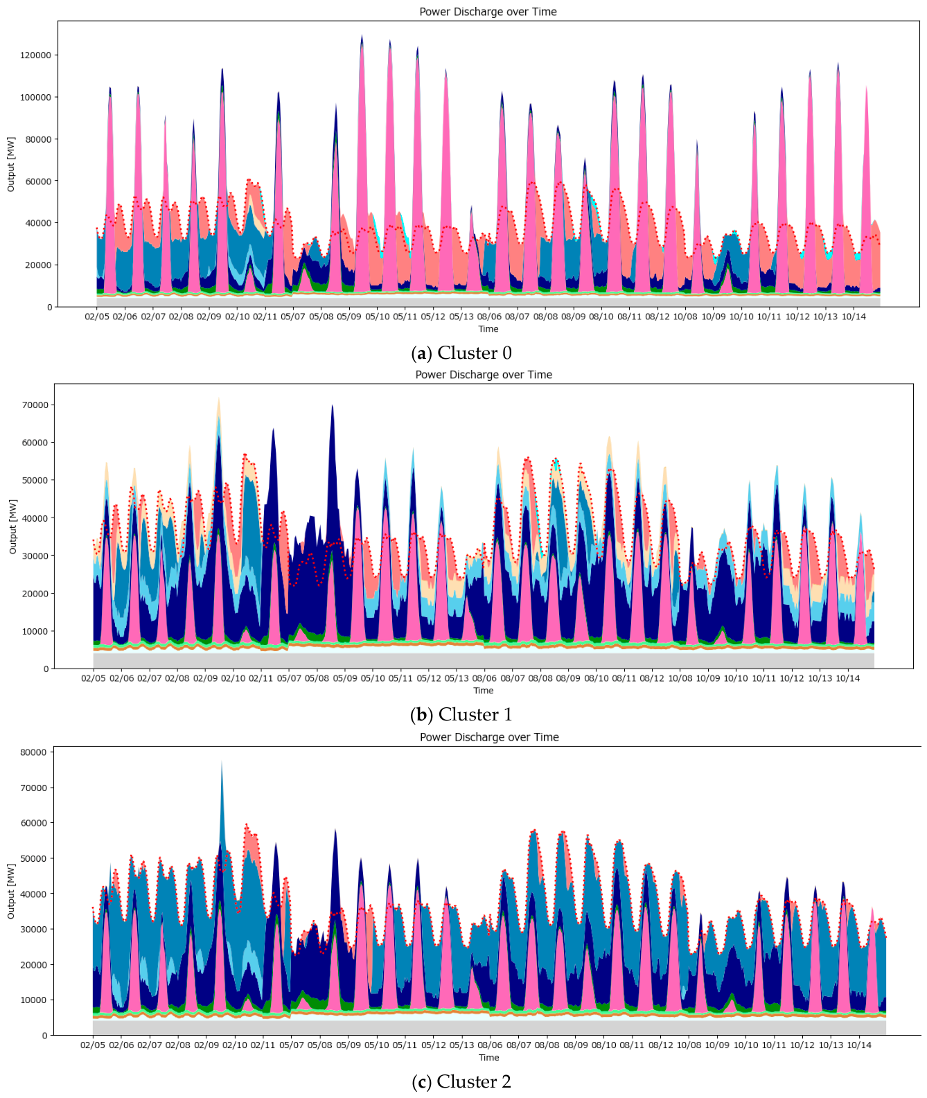
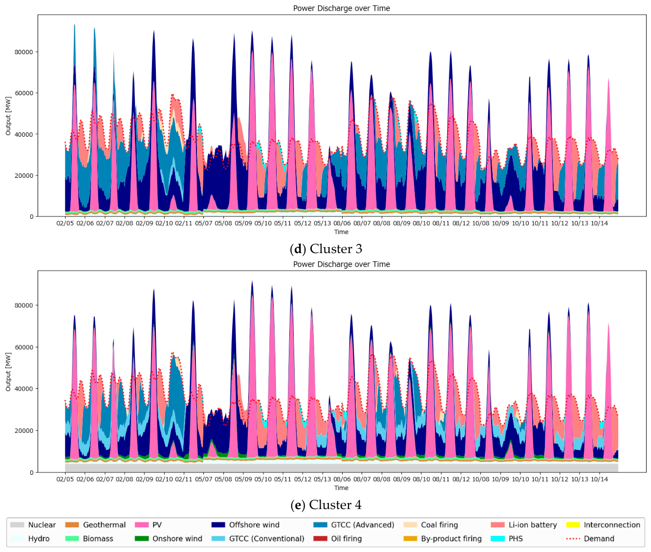
Appendix B.4. Range of Feasible Conditions Under Threshold Variation
Figure A2, Figure A3, Figure A4, Figure A5 and Figure A6 show, for each cluster, how the feasible ranges of principal parameters related to external factors change as the total-cost threshold varies. The ranges shown here aggregate the minimum, median, maximum, and mean of each parameter across the individuals realized below the threshold; a value falling within the indicated range does not in itself guarantee that individuals exist. In addition, because the number of realized individuals decreases as the threshold is tightened, some median values may exhibit instability due to small sample sizes. With these caveats in mind, these figures should be interpreted as conveying the directions in which conditions tend to be required for each type to be realized at lower cost.
Appendix B.4.1. Tendencies Common Across All Clusters
The most clearly evident common tendency across all clusters concerns the H2 price. As the total-cost threshold is tightened, the maximum H2 price decreases in many clusters, and the mean decreases continuously. That is, the H2 price is a representative constraint that influences low-cost realization across all types.
Appendix B.4.2. Cluster-Specific Characteristics
- Cluster 0: The realization ranges of the construction costs of PV and Li-ion battery tend to narrow, suggesting that, for the PV-led type to be realized at low cost, relatively low deployment costs of PV and battery storage are important.
- Cluster 1: The narrowing of the range of construction costs of offshore wind is particularly pronounced; for the offshore wind-led type, the cost of offshore wind acts as a decisive constraint.
- Cluster 2: The realization ranges of the construction costs of Li-ion battery and offshore wind tend to narrow, indicating that, in addition to the cost on the flexibility-provision side, the cost on the renewables side is also important for realizing the battery-centric type at low cost.
- Cluster 3: In addition to the H2 price, multiple fuel prices and construction costs - including the e-methane price, the NH3 price, the construction cost of offshore wind, and the construction cost of Li-ion battery - are simultaneously narrowed; this cluster therefore faces more multifaceted constraints for low-cost realization than the other clusters.
- Cluster 4: The narrowing of the H2 price range is the most pronounced, whereas relatively wide ranges are admissible for the other parameters; in the GTCC plus CO2 storage type, the H2 price appears to act as the dominant constraint.
Figure A2.
Feasible ranges of representative parameters for Cluster 0 under varying total-cost thresholds. The horizontal axis shows the total-cost threshold, and the vertical axis shows the value of each parameter. The lines indicate the minimum, median, maximum, and mean values among feasible individuals in Cluster 0.
Figure A2.
Feasible ranges of representative parameters for Cluster 0 under varying total-cost thresholds. The horizontal axis shows the total-cost threshold, and the vertical axis shows the value of each parameter. The lines indicate the minimum, median, maximum, and mean values among feasible individuals in Cluster 0.
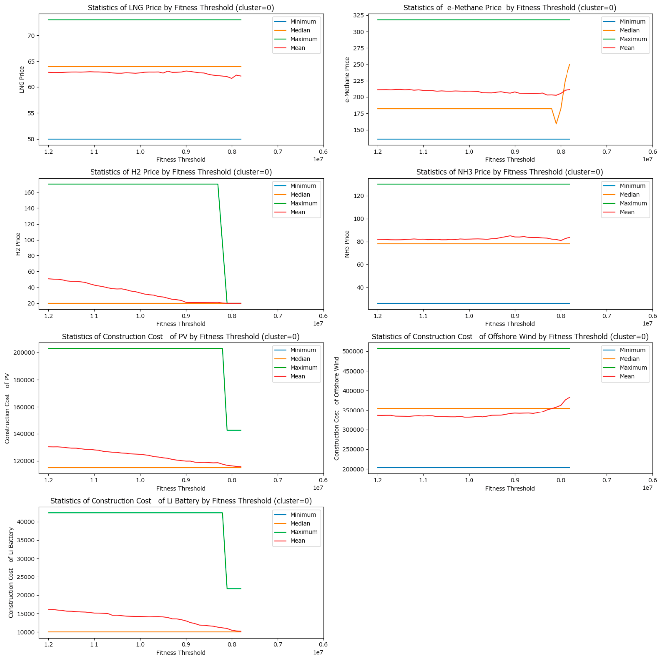
Figure A3.
Feasible ranges of representative parameters for Cluster 1 under varying total-cost thresholds. The horizontal axis shows the total-cost threshold, and the vertical axis shows the value of each parameter. The lines indicate the minimum, median, maximum, and mean values among feasible individuals in Cluster 1.
Figure A3.
Feasible ranges of representative parameters for Cluster 1 under varying total-cost thresholds. The horizontal axis shows the total-cost threshold, and the vertical axis shows the value of each parameter. The lines indicate the minimum, median, maximum, and mean values among feasible individuals in Cluster 1.
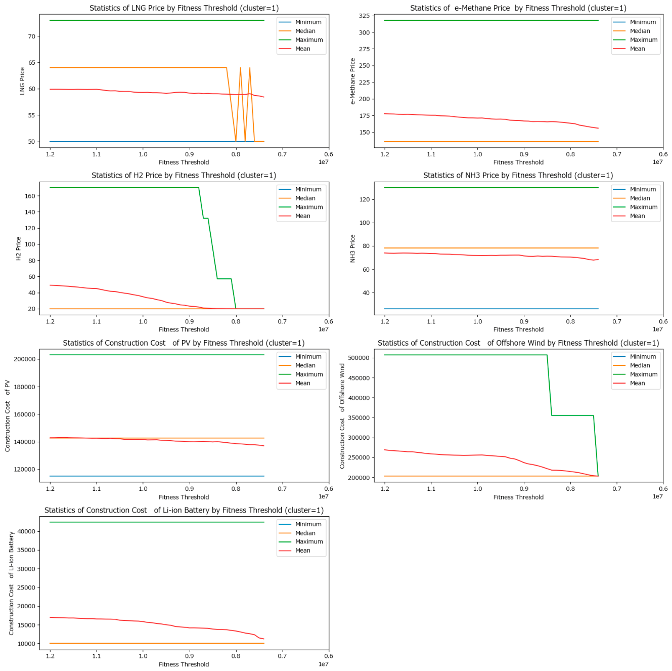
Figure A4.
Feasible ranges of representative parameters for Cluster 2 under varying total-cost thresholds. The horizontal axis shows the total-cost threshold, and the vertical axis shows the value of each parameter. The lines indicate the minimum, median, maximum, and mean values among feasible individuals in Cluster 2.
Figure A4.
Feasible ranges of representative parameters for Cluster 2 under varying total-cost thresholds. The horizontal axis shows the total-cost threshold, and the vertical axis shows the value of each parameter. The lines indicate the minimum, median, maximum, and mean values among feasible individuals in Cluster 2.
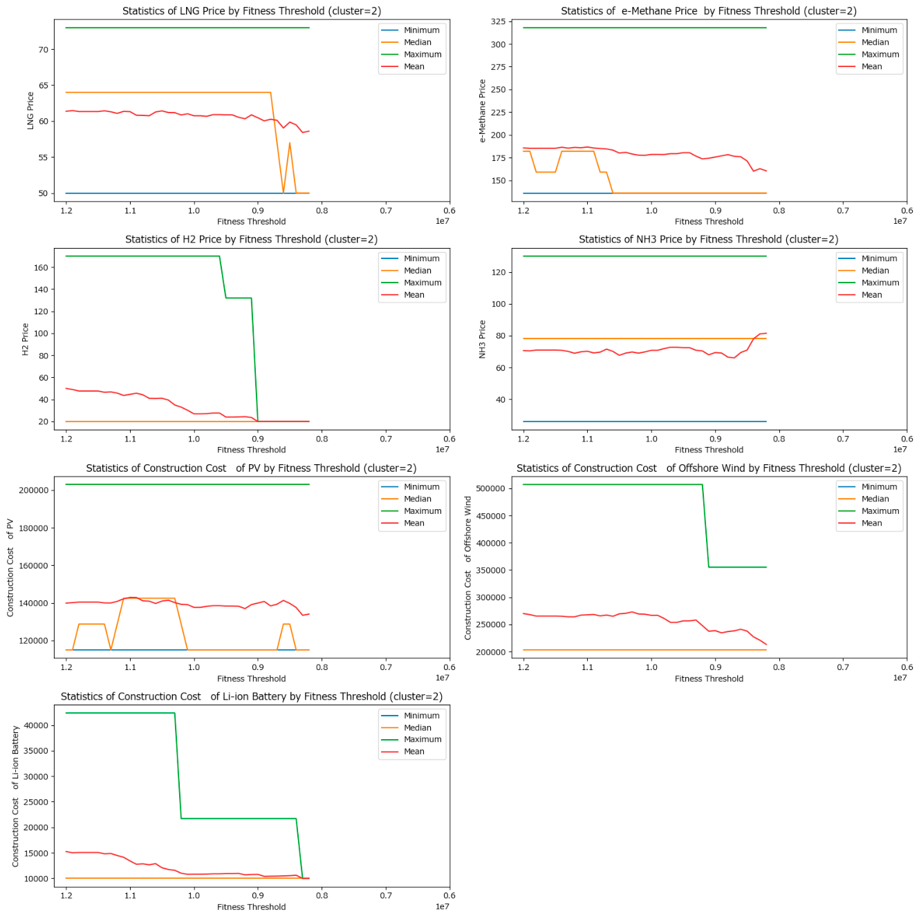
Figure A5.
Feasible ranges of representative parameters for Cluster 3 under varying total-cost thresholds. The horizontal axis shows the total-cost threshold, and the vertical axis shows the value of each parameter. The lines indicate the minimum, median, maximum, and mean values among feasible individuals in Cluster 3.
Figure A5.
Feasible ranges of representative parameters for Cluster 3 under varying total-cost thresholds. The horizontal axis shows the total-cost threshold, and the vertical axis shows the value of each parameter. The lines indicate the minimum, median, maximum, and mean values among feasible individuals in Cluster 3.
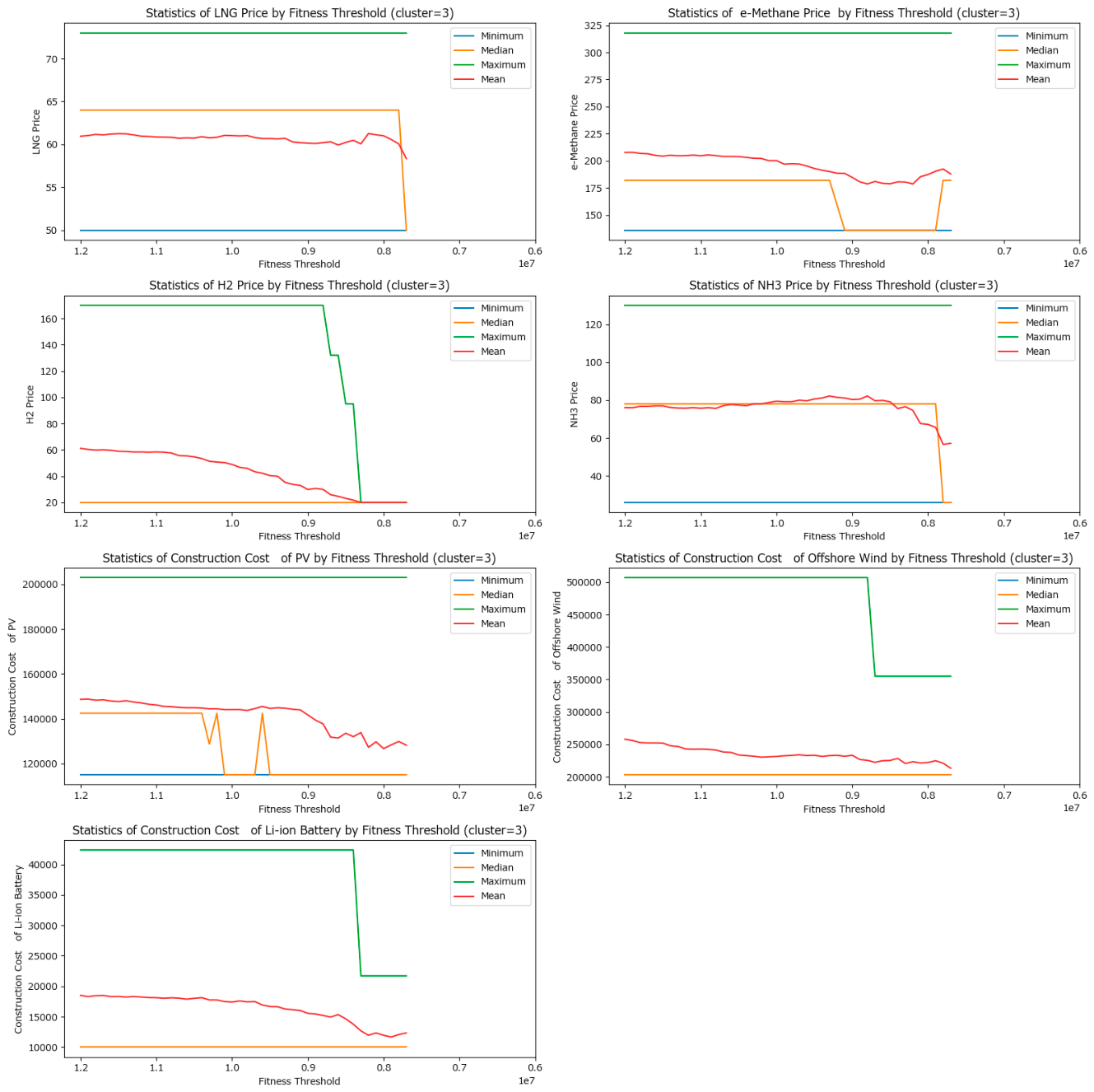
Figure A6.
Feasible ranges of representative parameters for Cluster 4 under varying total-cost thresholds. The horizontal axis shows the total-cost threshold, and the vertical axis shows the value of each parameter. The lines indicate the minimum, median, maximum, and mean values among feasible individuals in Cluster 4.
Figure A6.
Feasible ranges of representative parameters for Cluster 4 under varying total-cost thresholds. The horizontal axis shows the total-cost threshold, and the vertical axis shows the value of each parameter. The lines indicate the minimum, median, maximum, and mean values among feasible individuals in Cluster 4.
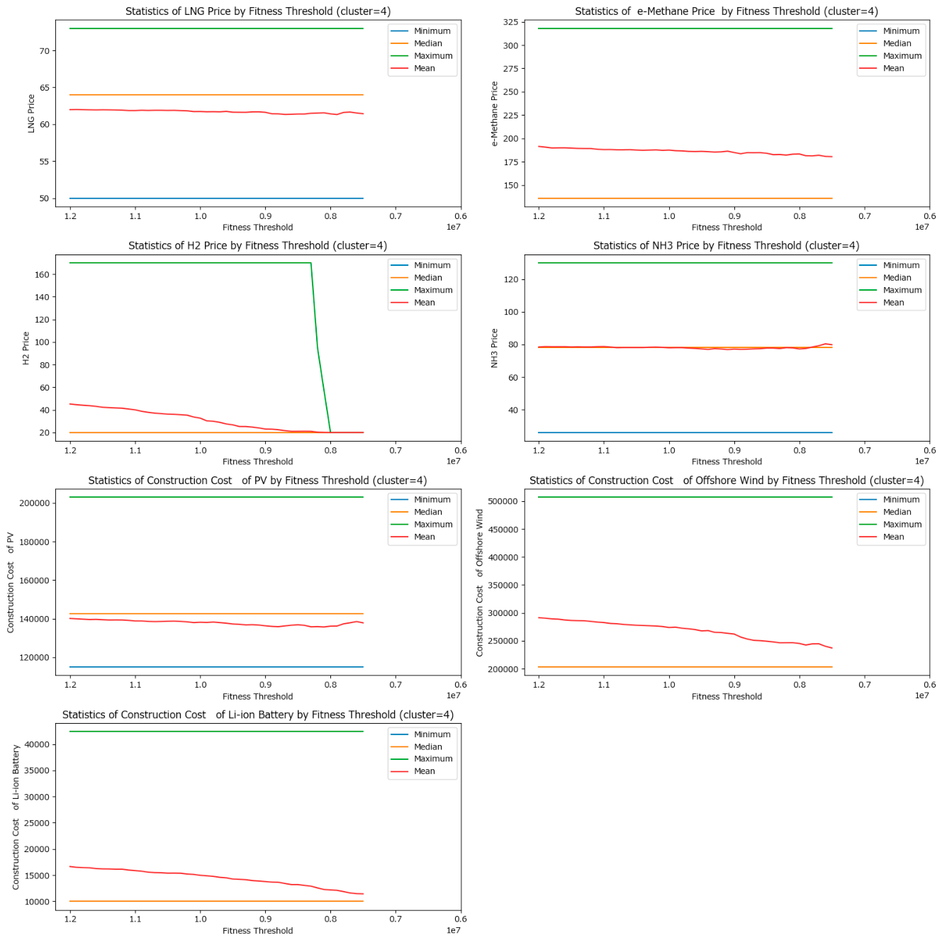
Appendix C. Detailed Analysis of Common and Variable Elements
This appendix presents the detailed discussion of the common and variable elements summarized in Section 3.4. The contents below are results obtained in the present demonstration and do not constitute universal claims under realistic conditions.
Appendix C.1. Common Elements
A comparison of the five representative clusters shown in Table 1 and Appendix B identifies the following elements as relatively robust requirements for achieving net-zero by 2050.
Appendix C.1.1. Deployment of Renewables at or Above a Certain Scale
All five scenarios make use of PV, offshore wind, or both to a certain extent, and configurations with almost no reliance on renewable energy do not appear among the representative scenarios. This indicates that, to achieve net-zero, the deployment of renewable energy is not an option specific to any single scenario but a foundational element common to multiple realization patterns.
Appendix C.1.2. Securing of Flexibility for Supply–Demand Fluctuations
Although the source of flexibility differs across scenarios, every scenario secures flexibility in some form. Specifically, supply–demand adjustment is performed by battery storage and GTCC in the PV-led with battery-backup type, by GTCC in the offshore wind-led type, by large-scale Li-ion battery in the battery-centric flexibility type, by limited GTCC and battery storage in the low-GTCC with variable renewables type, and by GTCC in the GTCC with CO2 storage type. That is, while flexibility itself is indispensable, the principal means of providing it varies across scenarios.
Appendix C.1.3. Importance of the H2 Price as a Condition for Low-Cost Realization
As shown in Appendix B.4.1, when the total-cost threshold is tightened, the admissible range of the H2 price narrows in many clusters; the H2 price thus stands out as a principal driver of cost structure common across scenarios. This suggests that the conditions of hydrogen procurement and price formation are cross-cutting factors that influence the realizability of future net-zero systems.
Appendix C.2. Variable Elements
Appendix C.2.1. The Principal Renewable Technology
PV plays the leading role in the PV-led with battery-backup type, whereas offshore wind has a higher share in the offshore wind-led type and the low-GTCC with variable renewables type. Although renewable deployment is indispensable for achieving net zero, whether its core technology is PV or offshore wind can vary across scenarios.
Appendix C.2.2 .The Approach to Providing Flexibility
In the battery-centric flexibility type, the Li-ion battery plays the central role, whereas in the GTCC with CO2 storage type, GTCC is the principal source of flexibility. In the PV-led with battery-backup type, battery storage is important in a complementary role, and in the offshore wind-led type, the complementary role of GTCC is more prominent. In other words, securing flexibility is a common task, but whether it is provided primarily by battery storage, primarily by GTCC, or by a combination of the two constitutes a variable element.
Appendix C.2.3. Extent of CO2 Storage Capacity Utilization
The low-GTCC with variable renewables type and the GTCC with CO2 storage type are characterized by relatively high upper limits of CO2 storage; in the latter, in particular, the combination of high-efficiency GTCC and CO2 storage capacity forms the foundation for scenario realization. By contrast, reliance on CO2 storage capacity is relatively low in the PV-led with battery-backup type and the offshore wind-led type. The extent to which CO2 management is positioned at the core of the system can therefore be understood as a difference among scenarios.
Appendix C.2.4. Combinations of Conditions That Tighten for Low-Cost Realization
The conditions that act as constraints on low-cost realization differ by scenario: the construction costs of PV and Li-ion battery in the PV-led with battery-backup type; the construction cost of offshore wind in the offshore wind-led type; the construction costs of Li-ion battery and offshore wind in the battery-centric flexibility type; multiple fuel prices and construction costs in the low-GTCC with variable renewables type; and primarily the H2 price in the GTCC with CO2 storage type (see Appendix B.4.2 for details).
Appendix C.3. Implications for Application
The analyses in Appendices C.1 to C.3 yield the following implications.
What is robustly required for achieving net-zero by 2050 comprises the deployment of renewable energy, the securing of flexibility, and favorable H2 price conditions. By contrast, whether the supply structure is centered on PV, on offshore wind, on battery storage for flexibility, or on GTCC together with CO2 storage remains a variable element. This implies that the pathway to net-zero is not unique: on top of foundational elements that must be secured across all scenarios, multiple technology portfolios and transition pathways may be realized.
Accordingly, the five representative scenarios extracted in this study can be understood as a comparative framework for organizing "which elements are essential and which admit room for choice." In practical terms, the common elements may be regarded as robust targets for investment and policy that should be secured with priority, while the variable elements may be positioned as a domain of choice to be selected flexibly in response to future changes in prices, institutions, technological progress, and social acceptability.
It should be noted, however, that the specific contents of the common and variable elements presented in this appendix, as well as the interpretation of construction costs as proxy variables, are results obtained in a demonstration under hypothetical conditions and do not constitute universal claims under realistic conditions. When the framework is applied to actual investment decision-making, an examination tailored to realistic conditions is required.
References
- Ministry of Economy Trade and Industry Green Growth Strategy Through Achieving Carbon Neutrality in 2050; 2021.
- Yamamoto, H. Research Direction of Energy Supply and Demand Models for Japan toward Realizing Carbon Neutrality by 2050-1. Rev. J. Inst. Electr. Eng. Jpn. 2023, 143, 70. [Google Scholar] [CrossRef]
- Akimoto, K.; Sano, F.; Takashi, H.; Oda, J.; Nagashima, M.; Kii, M. Estimates of GHG Emission Reduction Potential by Country, Sector, and Cost. Energy Policy 2010, 38, 3384–3393. [Google Scholar] [CrossRef]
- Akimoto, K.; Sano, F.; Junichiro, O.; Haruo, K.; Yuko, N. Climate Change Mitigation Measures for Global Net-Zero Emissions and the Roles of CO2 Capture and Utilization and Direct Air Capture. Energy Clim. Chang. 2021, 2. [Google Scholar] [CrossRef]
- Matsuo, Y. Research Direction of Energy Supply and Demand Models for Japan toward Realizing Carbon Neutrality by 2050-3. Inst. Energy Econ. Jpn. (IEEJ) IEEJ-NE Model. J. Inst. Electr. Eng. Jpn. 2023, 143, 75–78. [Google Scholar] [CrossRef]
- Inoue, T.; Kurosawa, A.; Kato, E.; Iwafune, Y.; Ogimoto, K.; Yamaguchi, Y.; Uchida, H.; Ota, Y.; Shimoda, Y. Energy Analysis in 2050 by Soft-Link ( 1 ) Scenarios Considering D Emand C Hange in C Onsumer-Sector and Their E Valuation. 2023, 44. [Google Scholar]
- Ogimoto, K.; Iwafune, Y.; Takeuchi, T.; Segawa, S.; Azuma, H.; Inoue, T.; Kurosawa, A.; Kato, E.; Yamaguchi, Y.; Uchida, H.; et al. Energy Analysis in 2050 by Soft-Link: (2) Impact of Demand Change in Residential and Commercial Sector on Power Demand and Supply. J. Jpn. Soc. Energy Resour. 2023, 44, 245–254. [Google Scholar]
- Brill, E.D.; Chang, S.Y.; Hopkins, L.D. Modeling To Generate Alternatives: The Hsj Approach and an Illustration Using a Problem in Land Use Planning. Manag. Sci. 1982, 28, 221–235. [Google Scholar] [CrossRef]
- DeCarolis, J.F. Using Modeling to Generate Alternatives (MGA) to Expand Our Thinking on Energy Futures. Energy Econ. 2011, 33, 145–152. [Google Scholar] [CrossRef]
- Price, J.; Keppo, I. Modelling to Generate Alternatives: A Technique to Explore Uncertainty in Energy-Environment-Economy Models. Appl. Energy 2017, 195, 356–369. [Google Scholar] [CrossRef]
- Neumann, F.; Brown, T. The Near-Optimal Feasible Space of a Renewable Power System Model. Electr. Power Syst. Res. 2021, 190. [Google Scholar] [CrossRef]
- Lau, M.; Patankar, N.; Jenkins, J.D. Measuring Exploration: Review and Systematic Evaluation of Modelling to Generate Alternatives Methods in Macro-Energy Systems Planning Models. ArXiv 2024. [Google Scholar]
- Yokoyama, R.; Shinano, Y.; Taniguchi, S.; Ohkura, M.; Wakui, T. Optimization of Energy Supply Systems by MILP Branch and Bound Method in Consideration of Hierarchical Relationship between Design and Operation. Energy Convers. Manag. 2015, 92, 92–104. [Google Scholar] [CrossRef]
- Wakui, T.; Hashiguchi, M.; Sawada, K.; Yokoyama, R. Two-Stage Design Optimization Based on Artificial Immune System and Mixed-Integer Linear Programming for Energy Supply Networks. Energy 2019, 170, 1228–1248. [Google Scholar] [CrossRef]
- Yokoyama, R.; Shinano, Y.; Taniguchi, S.; Wakui, T. Search for K-Best Solutions in Optimal Design of Energy Supply Systems by an Extended MILP Hierarchical Branch and Bound Method. Energy 2019, 184, 45–57. [Google Scholar] [CrossRef]
- Holland, J.H. Adaptation in Natural and Artificial Systems; University of Michigan Press: Ann Arbor, 1975; ISBN 9780472084609. [Google Scholar]
- Goldberg, D.E. Genetic Algorithms in Search, Optimization, and Machine Learning; Addison-Wesley: Reading, MA, 1989; ISBN 9780201157673. [Google Scholar]
- Lundberg, S.M.; Lee, S.I. A Unified Approach to Interpreting Model Predictions. Proc. Adv. Neural Inf. Process. Syst. 2017, Vol. 2017-Decem, 4766–4775. [Google Scholar]
- Fortin, F.A.; De Rainville, F.M.; Gardner, M.A.; Parizeau, M.; Gagńe, C. DEAP: Evolutionary Algorithms Made Easy. J. Mach. Learn. Res. 2012, 13, 2171–2175. [Google Scholar]
- DEAP Development Team DEAP Documentation. Available online: https://deap.readthedocs.io/en/master/ (accessed on 24 June 2026).
- Breiman, L. Random Forests. Mach. Learn. 2001, 45, 5–32. [Google Scholar] [CrossRef]
- Pedregosa, F.; Varoquaux, G.; Gramfort, A.; Michel, V.; Thirion, B.; Grisel, O.; Blondel, M.; Prettenhofer, P.; Weiss, R.; Dubourg, V.; et al. Scikit-Learn: Machine Learning in Python. J. Mach. Learn. Res. 2011, 12, 2825–2830. [Google Scholar]
- Kuwabara, T.; Mohr, D.; Sauer, B.; Yamada, Y. How Jpn. Could Reach Carbon Neutrality By 2050 2021.
- Industry, M. of E.T. and Green Transformation Budget and Policy Measures Available online: https://www.meti.go.jp/policy/energy_environment/global_warming/gx_budget.html (accessed on 3 May 2026).
- Ministry of Land, I.T. and T. Current Status of the Environmental Sector in the Capital Region; 2022.
- Agency for Natural Resources and Energy Power Generation Cost Verification Working Group (FY2021), Document No. 8-6; 2021.
- International Renewable Energy Agency Electricity Storage and Renewables: Costs and Markets to 2030; 2017.
- JERA Thermal Power Plants List. Available online: https://www.jera.co.jp/en/corporate/business/thermal-power/list/ (accessed on 24 February 2026).
- Tokyo Gas Power Sources for Electricity Generation. Available online: https://home.tokyo-gas.co.jp/gas_power/plan/power/source.html (accessed on 26 June 2026).
- Tokyo Electric Power Company Holdings Electricity Demand and Supply Forecast for TEPCO Service Area. Available online: https://www.tepco.co.jp/forecast/html/area_jukyu_p-j.htm (accessed on 25 February 2026).
- Agency for Natural Resources and Energy Nuclear Energy Policy and Current Status; 2023.
- Ministry of the Environment Japan Environmental Data Repository (REPOS). Available online: https://repos.env.go.jp/web/ (accessed on 25 April 2026).
- The Institute of Energy Economics Japan Evaluation of the Potential for Introducing Solar Power Generation, Taking into Account Local Regulations and Building Characteristics; 2023.
- Renewable Energy Institute Basic Information on Wind Power Generation; 2024.
- Agency for Natural Resources and Energy Comprehensive Energy Statistics of Japan (STTE 028); 2023.
- Ministry of the Environment Japan Greenhouse Gas Emissions Calculation and Reporting System. Available online: https://policies.env.go.jp/earth/ghg-santeikohyo/calc.html (accessed on 25 February 2026).
- Power Producer and Supplier Network Statistics on Gas Prices and Supply. Available online: https://pps-net.org/statistics/gas6 (accessed on 25 February 2026).
- The Institute of Energy Economics Japan Economic and Environmental Evaluation of Hydrogen Carriers from Overseas Production to Domestic End-Use; 2023.
- Japan Science and Technology Agency; Center for Low Carbon Society Strategy Cost and Evaluation of the Direct Air Capture (DAC) Method for Carbon Dioxide (Vol. 2); 2020.
- Agency for Natural Resources and Energy Summary of the Final Report of the CCS Long-Term Roadmap Review Committee; 2023.
Figure 1.
Conceptual structure of the proposed framework. The framework consists of a hierarchical inverse analysis model that integrates upper-level GA-based exploration of exogenous assumptions with lower-level LP-based operational optimization, followed by sensitivity analysis and representative-scenario extraction from the generated feasible solution set.
Figure 1.
Conceptual structure of the proposed framework. The framework consists of a hierarchical inverse analysis model that integrates upper-level GA-based exploration of exogenous assumptions with lower-level LP-based operational optimization, followed by sensitivity analysis and representative-scenario extraction from the generated feasible solution set.
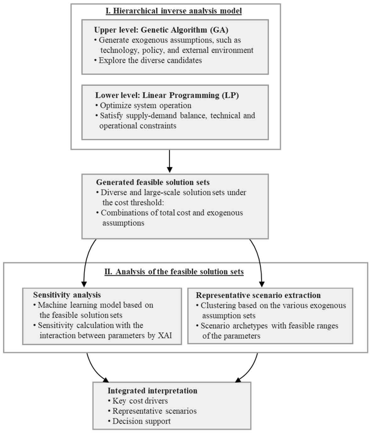
Figure 2.
Overview of the proposed GA–LP integrated framework. The upper-level genetic algorithm (GA) explores combinations of exogenous conditions, while the lower-level linear programming (LP) model evaluates each individual by optimizing system operation under technical and supply–demand constraints. For each individual, the total cost is calculated by combining OPEX from the LP model with CAPEX and O&M costs. Individuals whose total cost falls below a predefined threshold are retained, and the GA generates the next population through selection, crossover, and mutation. Repeating this process yields diverse feasible total cost–condition pairs.
Figure 2.
Overview of the proposed GA–LP integrated framework. The upper-level genetic algorithm (GA) explores combinations of exogenous conditions, while the lower-level linear programming (LP) model evaluates each individual by optimizing system operation under technical and supply–demand constraints. For each individual, the total cost is calculated by combining OPEX from the LP model with CAPEX and O&M costs. Individuals whose total cost falls below a predefined threshold are retained, and the GA generates the next population through selection, crossover, and mutation. Repeating this process yields diverse feasible total cost–condition pairs.
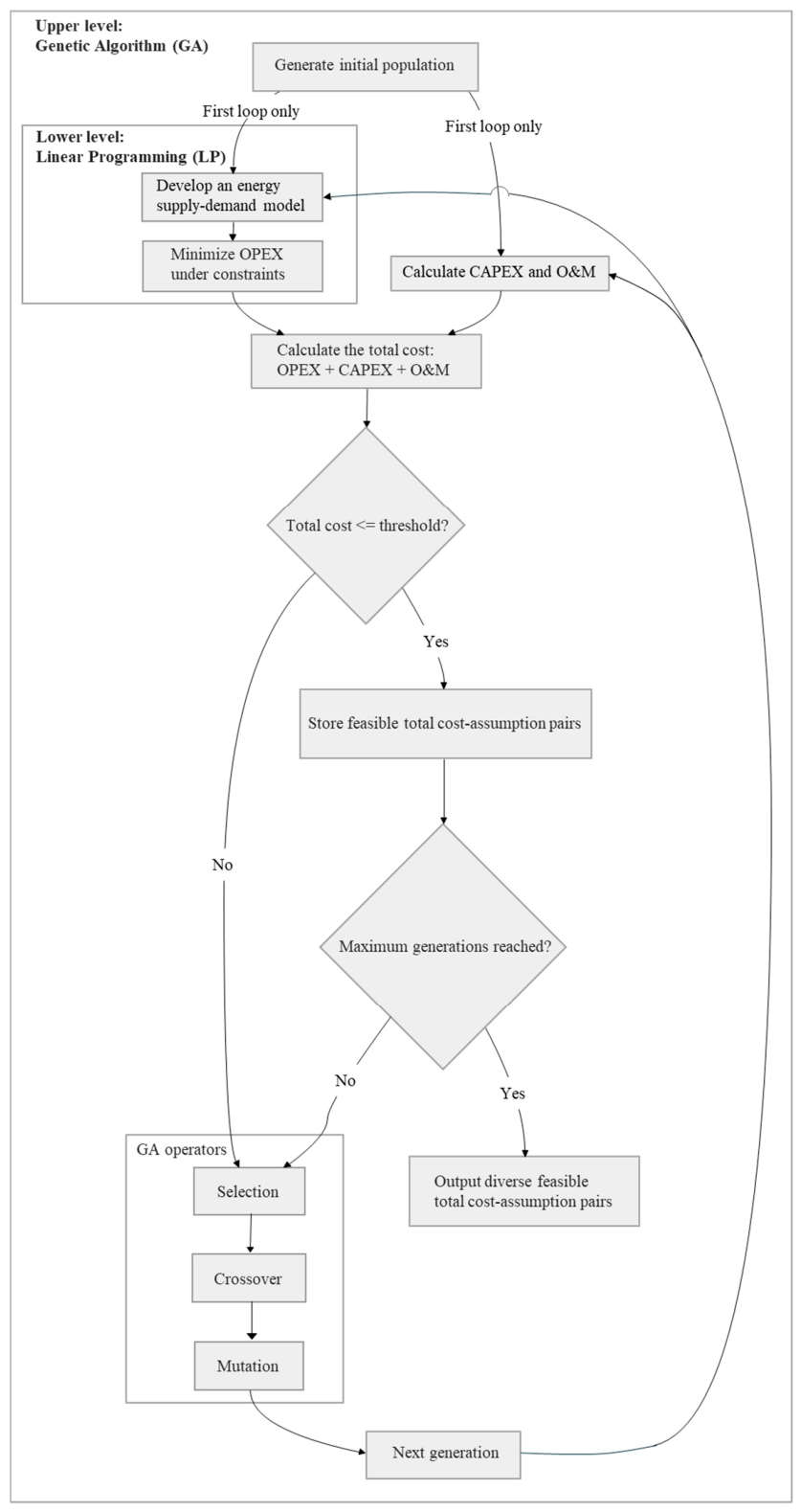
Figure 3.
Conceptual structure of the regional energy supply–demand model used in the demonstration. The figure illustrates the relationships among primary energy inputs, conversion technologies, storage and transport, final energy demand, and carbon management options, including CCS and DACCS.
Figure 3.
Conceptual structure of the regional energy supply–demand model used in the demonstration. The figure illustrates the relationships among primary energy inputs, conversion technologies, storage and transport, final energy demand, and carbon management options, including CCS and DACCS.
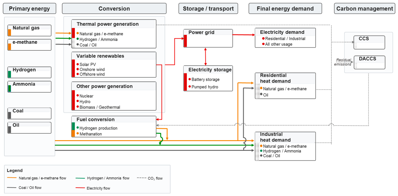
Figure 4.
Distribution of feasible individuals by total cost. The horizontal axis shows the index of feasible individuals in the order in which they were retained during the GA search, and the vertical axis shows the total cost (fitness value). The figure indicates that lower-cost feasible individuals emerge as the search progresses, while a wide range of feasible solutions remains below the cost threshold.
Figure 4.
Distribution of feasible individuals by total cost. The horizontal axis shows the index of feasible individuals in the order in which they were retained during the GA search, and the vertical axis shows the total cost (fitness value). The figure indicates that lower-cost feasible individuals emerge as the search progresses, while a wide range of feasible solutions remains below the cost threshold.
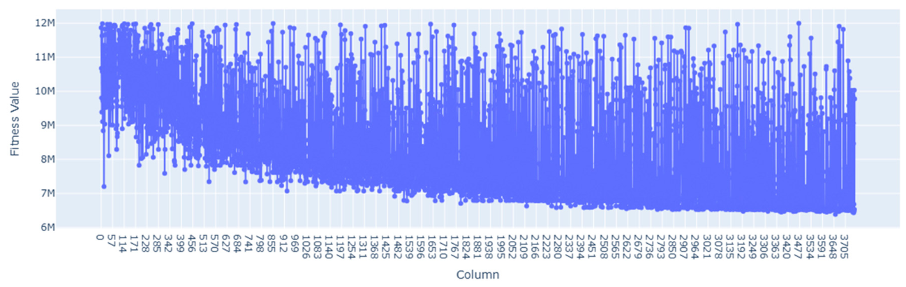
Figure 5.
Relationship between the novelty of explanatory-variable combinations and total cost for feasible individuals. Each point represents one feasible individual, with the horizontal axis showing the distance-based novelty score and the vertical axis showing the total cost. The novelty score is defined as the mean Manhattan distance to the 10 nearest neighbors in the min–max normalized explanatory-variable space, divided by the number of explanatory variables. The solid line shows the median total cost within each novelty decile, and the shaded area indicates the 10th–90th percentile range.
Figure 5.
Relationship between the novelty of explanatory-variable combinations and total cost for feasible individuals. Each point represents one feasible individual, with the horizontal axis showing the distance-based novelty score and the vertical axis showing the total cost. The novelty score is defined as the mean Manhattan distance to the 10 nearest neighbors in the min–max normalized explanatory-variable space, divided by the number of explanatory variables. The solid line shows the median total cost within each novelty decile, and the shaded area indicates the 10th–90th percentile range.
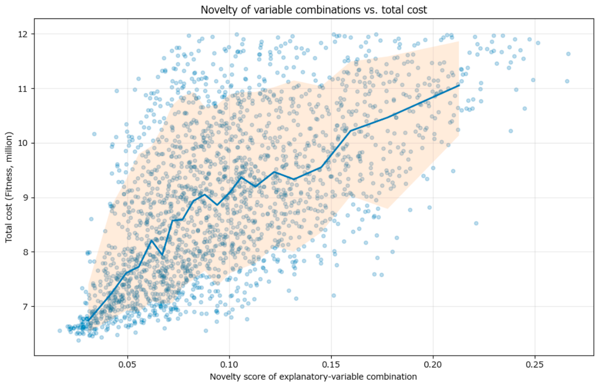
Figure 6.
High-importance parameters and their SHAP-value distributions. Panel (a) shows the top 10 parameters ranked by mean absolute SHAP value, where the horizontal axis indicates the average magnitude of impact on the model output and the vertical axis lists the parameters. Panel (b) shows the SHAP-value distribution for the same parameters, where each point represents one feasible individual, the horizontal axis shows the SHAP value, and the color indicates the feature value.
Figure 6.
High-importance parameters and their SHAP-value distributions. Panel (a) shows the top 10 parameters ranked by mean absolute SHAP value, where the horizontal axis indicates the average magnitude of impact on the model output and the vertical axis lists the parameters. Panel (b) shows the SHAP-value distribution for the same parameters, where each point represents one feasible individual, the horizontal axis shows the SHAP value, and the color indicates the feature value.
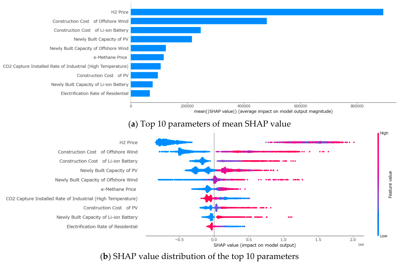
Figure 7.
SHAP dependence plots for representative parameters. In each panel, the horizontal axis shows the value of the focal parameter, and the vertical axis shows its SHAP value. The color indicates the interacting parameter with the strongest interaction effect. Panels (a)–(d) correspond to the H2 price, construction cost of offshore wind, construction cost of Li-ion battery and newly built capacity of PV, respectively.
Figure 7.
SHAP dependence plots for representative parameters. In each panel, the horizontal axis shows the value of the focal parameter, and the vertical axis shows its SHAP value. The color indicates the interacting parameter with the strongest interaction effect. Panels (a)–(d) correspond to the H2 price, construction cost of offshore wind, construction cost of Li-ion battery and newly built capacity of PV, respectively.
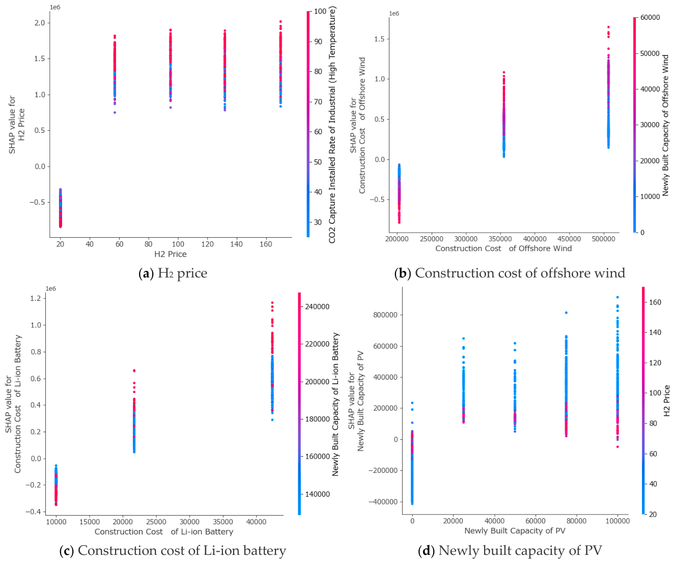
Figure 8.
Number of feasible individuals by cluster. The horizontal axis shows the cluster ID, and the vertical axis shows the number of feasible individuals assigned to each cluster. The figure illustrates that feasible solutions are unevenly distributed across clusters, indicating differences in the frequency with which each representative solution type appears.
Figure 8.
Number of feasible individuals by cluster. The horizontal axis shows the cluster ID, and the vertical axis shows the number of feasible individuals assigned to each cluster. The figure illustrates that feasible solutions are unevenly distributed across clusters, indicating differences in the frequency with which each representative solution type appears.
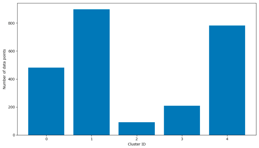
Figure 9.
Distribution of total cost by cluster. The horizontal axis shows the cluster ID, and the vertical axis shows the total cost (fitness value). The boxplots indicate differences among clusters in median cost level and within-cluster variability, suggesting that the extracted clusters represent solution types with distinct cost structures.
Figure 9.
Distribution of total cost by cluster. The horizontal axis shows the cluster ID, and the vertical axis shows the total cost (fitness value). The boxplots indicate differences among clusters in median cost level and within-cluster variability, suggesting that the extracted clusters represent solution types with distinct cost structures.
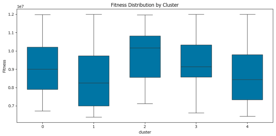
Figure 10.
Heatmap of standardized mean values of major equipment-related parameters by cluster. The horizontal axis shows the cluster ID, and the vertical axis shows the major parameters used for clustering. Each cell reports the mean standardized value of the corresponding parameter within the cluster, where positive values indicate levels above the overall mean and negative values indicate levels below the overall mean. The figure highlights distinct equipment-configuration characteristics across the five representative clusters.
Figure 10.
Heatmap of standardized mean values of major equipment-related parameters by cluster. The horizontal axis shows the cluster ID, and the vertical axis shows the major parameters used for clustering. Each cell reports the mean standardized value of the corresponding parameter within the cluster, where positive values indicate levels above the overall mean and negative values indicate levels below the overall mean. The figure highlights distinct equipment-configuration characteristics across the five representative clusters.
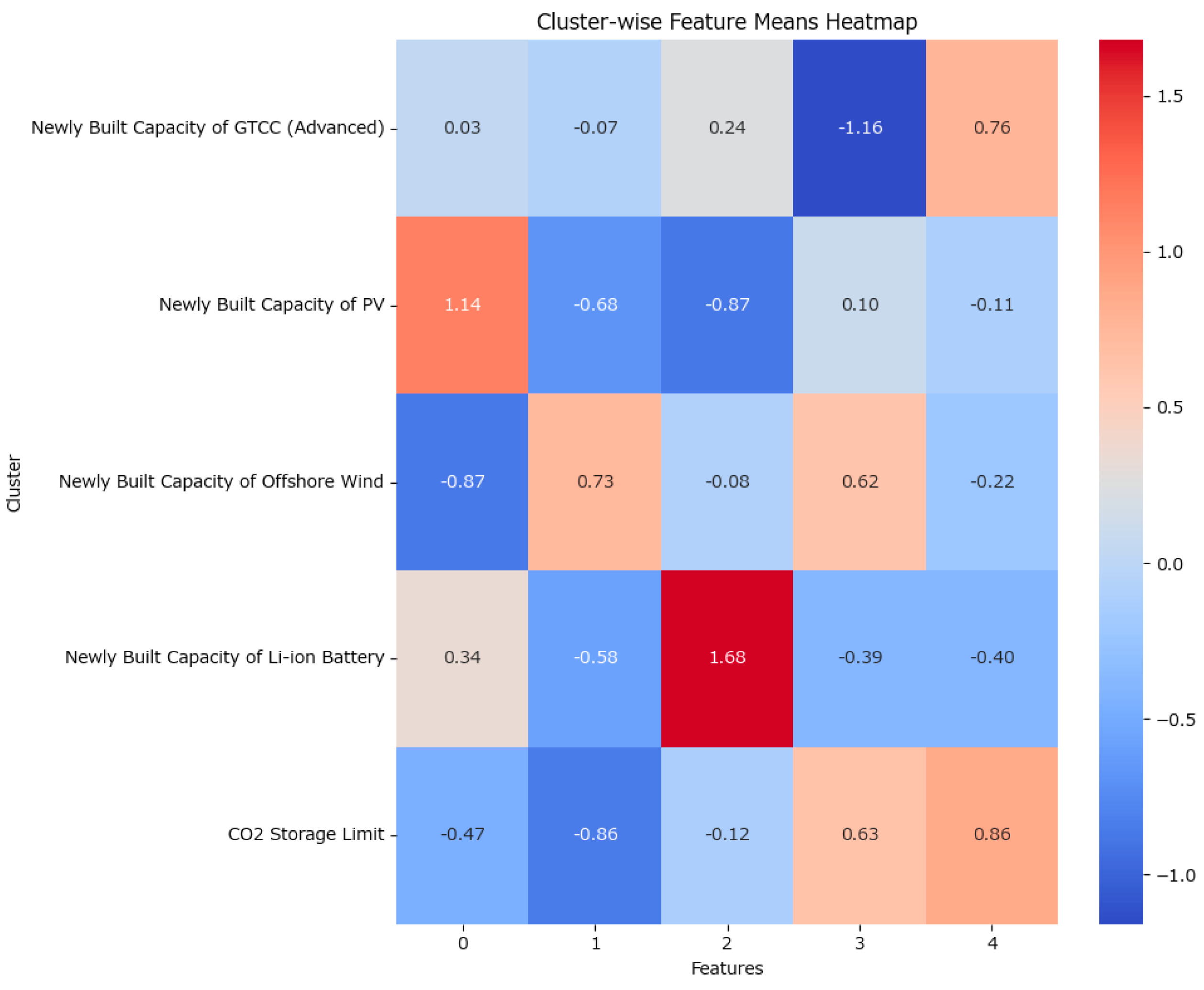
Table 1.
Cluster characteristics and representative scenario names.
| Cluster ID | Capacity Configuration | Operational Pattern | Key Conditions for Low-Cost Feasibility | Representative Scenario |
|---|---|---|---|---|
| 0 | High PV capacity; low offshore wind capacity | PV-centered supply complemented by GTCC and battery storage | PV construction cost; Li-ion battery construction cost | PV-led with battery backup |
| 1 | High offshore wind capacity | Offshore wind as baseline supplemented by GTCC | Offshore wind construction cost | Offshore wind-led |
| 2 | Prominently high Li-ion battery capacity | Battery-centered flexibility provision | Li-ion battery construction cost; H2 price; offshore wind construction cost | Battery-centric flexibility |
| 3 | Low high-efficiency GTCC; high offshore wind and CO2 storage | Variable renewable-dominant supply with limited GTCC backup | H2 price; e-methane price; NH3 price; offshore wind and Li-ion battery construction costs | Low-GTCC with variable renewables |
| 4 | High-efficiency GTCC and CO2 storage | GTCC-based stable supply | H2 price | GTCC with CO2 storage |
Disclaimer/Publisher’s Note: The statements, opinions and data contained in all publications are solely those of the individual author(s) and contributor(s) and not of MDPI and/or the editor(s). MDPI and/or the editor(s) disclaim responsibility for any injury to people or property resulting from any ideas, methods, instructions or products referred to in the content. |
© 2026 by the authors. Licensee MDPI, Basel, Switzerland. This article is an open access article distributed under the terms and conditions of the Creative Commons Attribution (CC BY) license.
Copyright: This open access article is published under a Creative Commons CC BY 4.0 license, which permit the free download, distribution, and reuse, provided that the author and preprint are cited in any reuse.