

Submitted:
20 May 2026
Posted:
21 May 2026
You are already at the latest version
Abstract
This paper shows how to treat quantum field theory as a modern, locally
Lorentz covariant quantum version of the classical, mechanical universe
suggested by Laplace over 200 years ago. The result is a fairly
common-sense single-history, single-world alternative to decoherent
histories (Gell-Mann and Hartle) and many-worlds interpretations
(Everett, DeWitt). From the assumption that there is a single universal
Heisenberg state whose N-point functions uniquely describe all
physical details of our universe, everything is rigorously deduced in a
way showing that the mathematical formalism is capable of yielding its
own interpretation. Probabilities arise from the neglect of the
environment in approximate models. By giving the collapse of the wave
function at a double slit a natural unitary explanation, new light is
shed on the quantum measurement problem and the origin of the Born rule.
Keywords:
universal quantum state
; quantum-classical transition
; maximum entropy principle
; coarse graining
; bistability
; chaos
; decoherent histories
; quantum cosmology
; double slit
; quantum measurement problem
1. Introduction
1.1. Quantum Cosmology
There is very wide agreement that quantum physics seems to be valid at all length and time scales, with the possible exception of effects near and below the Planck scale. Theoretical studies of the earliest stages of the universe require that quantum field theory applies to the universe as a whole (DeWitt [36], Hartle [68], Bojowald [17]). The conceptual foundations of quantum field theory are discussed in Cao [30] from the perspective of practitioners in the field. Since the universe is a closed system, it is almost generally assumed that its evolution is unitary. For lack of a consistent quantum theory of gravity, the latter is typically incorporated into quantum field theory in an approximate manner, as semiclassical gravity (Carlip [31]), effective field theory (Burgess [20]), low energy gravity (Wallace [123]), or stochastic gravity (Hu & Verdaguer [74]).
The mathematically more fertile applications of quantum mechanics to the dynamics of the universe employ either decoherence functionals on histories (or “worlds”), quantifying their degree of non-classicality (Dowker & Halliwell [41], Gell-Mann & Hartle [51,52], Griffiths [57], Halliwell [62], Hartle [68]), or influence functionals (Feynman & Vernon [46]), the logarithms of decoherence functionals, generalized to continuous histories. The latter are often presented in the closed time path framework (Chou et al. [35]), with fields in place of continuous histories (Calzetta & Hu [23,24,25,26], Halliwell [61], Hu [73], Isham & Linden [76]).
A flurry of recent activity is devoted to a possible justification of the quantum-classical transition through gravitational decoherence (e.g., Halliwell [61], Anastopoulos & Hu [4], Bassi et al. [8], Kanno et al. [79], Hsiang et al. [72]) or gravity-mediated decoherence (Moustos & Anastopoulos [95]). Here one treats the gravitational field as environment for some massive quantum system S, and derives, from typical assumptions of the theory of open quantum system (Breuer & Petruccione [18]), a reduced dissipative dynamics for S alone in terms of deterministic Lindblad master equations or stochastic Schrödinger–Langevin equations. These are then analyzed for decoherence effects, with an eye towards the emergence of classical properties and towards potential experiments capturing signals sensitive to quantum features of gravity.
As mentioned by Bassi et al. [8], “there is no unanimous theoretical description for gravitational decoherence. [...] quantum gravitational features are introduced in a rather ad-hoc manner.” For example, Chiarelli [34] starts with a nonrelativistic particle in an external potential, coupled to gravitation, then assumes in their Equation (5) that the total wave function factors into the product of a particle wave function and a gravitational wave function. Such a state cannot, however, be prepared since—unlike in a measurement context—the particle always interacts with the gravitational field. (The author gives on page 9 another reason for distrusting (5), namely “assuming the existence of separate systems and environments subtly introduces a classical condition into the nature of the overall supersystem.”) After further approximations he gets a nonrelativistic Langevin Equation (24). Later in (85), he has to smuggle in a finite propagation speed not present in the derived dynamics.
1.2. Eight Desiderata for a Realist Interpretation of Quantum Physics
In spite of 100 years of impressive advances since the modern mathematical form of quantum mechanics was discovered, physicists still disagree widely on what quantum mechanics says about reality (Gibney [53]). In particular, it is controversial how to interpret quantum fields, the quantum state of the universe, or even whether the latter concept makes sense at all. Widely differing views can be found, e.g., in Baker [6], Bunge [19], Chen [33], Dürr & Lazarovici [43], Hartle [68,69], Hobson [71], Kent [83], Kuhlmann et al. [86], Laloë [87], Maudlin [92], Swanson [118], Wallace [121,122], Wallace & Timpson [125].
The reason is that there is still a glaring gap in the understanding of quantum mechanics, called the measurement problem (Wheeler & Zurek [128], Allahverdyan et al. [2,3], Neumaier [99]). From today’s point of view, this is the problem of explaining, in terms of unitary dynamics only, why a quantum measurement device, specified in quantum mechanical terms, behaves according to the Born rule when interacting with a quantum system to be measured; and why the initial state of a quantum system changes, through interaction with a quantum measurement device, into a final state consistent with state reduction or collapse (in the sense described in Section 4.9 below).
A quantum treatment of the early universe requires an observer-independent view of quantum mechanics that allows one to discuss what actually happened long before any observers were present. Thus some form of scientific realism (Saunders [113], Fraser [49]) is required. An ideal interpretation of quantum physics suitable for quantum cosmology should satisfy most of the following list of desirable properties:
- 1.
- The mathematical formalism of quantum mechanics is sufficient as it stands. No metaphysics needs to be added to it.
- 2.
- It is unnecessary to introduce external observers or to postulate the existence of a realm where the laws of classical physics hold sway.
- 3.
- It makes sense to talk about a state for the whole universe.
- 4.
- This state never collapses, and hence the universe as a whole is rigorously deterministic.
- 5.
- The ergodic properties of laboratory measuring instruments are inessential to its foundations.
- 6.
- The statistical interpretation itself need not be imposed a priori.
- 7.
- The symbols of quantum mechanics represent reality just as much as do those of classical mechanics.
- 8.
- The mathematical formalism of the quantum theory is capable of yielding its own interpretation.
This list is taken almost verbatim from (DeWitt [37], p.167). [DeWitt has in points 3 and 4 more specifically ’state vector’ in place of ’state’, and in point 5 an additional side statement. Points 7 and 8 are not in his list but appear verbatim in his discussion on the subsequent page.]
Not surprisingly, the above desiderata are satisfied to a varying extent by different interpretations of quantum mechanics.
1.3. Structure of the Paper
In this paper, we present quantum field theory in a way that adds clarity and rigor to the analysis of classical and quantum features of the universe and its constituents. This might ultimately shed new light on the conundrums of quantum cosmology. A new, holistic view of the physical universe and its constituents is proposed, specified in a deductive way as a consequence of the assumption that there is a single universal Heisenberg state that uniquely describes all physical details of our universe. The approach is a locally Lorentz covariant quantum version of the classical, mechanical universe suggested by Laplace over 200 years ago. By reinterpreting some of the mathematical terms of quantum field theory, it provides a fairly common-sense single-history, single-world alternative to decoherent histories (Gell-Mann and Hartle) and many-worlds interpretations (Everett, DeWitt), compatible with scientific realism. The new view sheds a new light on the quantum measurement problem, illustrated here by giving the collapse of the wave function at a double slit a natural unitary explanation.
Section 2 shows how some traditional interpretations (many worlds, decoherent histories, Bohmian mechanics, and Copenhagen) fare when judged by DeWitt’s eight criteria. Section 3 gives an overview over the properties of the Laplacian quantum universe introduced in more detail in Section 4, discusses it in the light of DeWitt’s eight criteria, and compares its main features with those of traditional interpretations.
Section 4 is the formal core of the paper. It shows how to treat quantum field theory as a modern, locally Lorentz covariant quantum version of the classical, mechanical universe suggested by Laplace over 200 years ago.
In Section 4.1 we define model universes and quantum values, their local and nonlocal beables. Section 4.2 defines the formal specification of physical systems, and discusses how physical systems of interest in a laboratory get their properties from the universal quantum state. We also define what it means that one physical system knows anything about another physical system—an already classically nontrivial question. In Section 4.3 we discuss how the unitary dynamical law that governs the exact dynamics of the universe gives rise to (necessarily approximate) deterministic or stochastic equations of motion for all physical systems, and to the boundary conditions specifying the effects of their environment.
In Section 4.4 we specify the class of physical systems in a quantum field theory deserving to be called classical, in terms of local equilibrium states. Section 4.5 introduces the detector response principle defining the intrinsic meaning of quantum measurement and its implication, the Born rule for quantum measurements. Section 4.6 discusses the modern version of the collapse of the wave function (state reduction). As a specific example of the collapse, we give in SubSection 4.7Section 4.8 a detailed treatment of what happens when a quantum system passes a double slit, and how the observed collapse of the wave function arises from the unitary dynamics of simple models.
Section 4.9 develops transition operators, needed to work with stochastic processes in a quantum context. The final Section 4.10 shows how decoherent histories fit into the Laplacian quantum universe setting.
2. Interpretations of Quantum Mechanics
The physical facts observed in Nature, or deduced from observations, refer to theoretical concepts called beables (Bell [11]). What precisely these concepts are depends on the interpretation of quantum mechanics. We briefly look at some of these in the light of the eight desiderata from Section 1.2.
2.1. Many Worlds?
In many worlds interpretations (Everett [45], DeWitt [36], Wallace [122]), experimental results are interpreted to occur in one of the many worlds, depending on the particular outcomes. Thus the beables are the totality of worlds, forming a somewhat fuzzily defined branching web whose details depend on whom you ask. See, e.g., Blackshaw & Franklin [12] for the lack of consensus.
DeWitt [37] introduced his list of desiderata with the words, “my main purpose [...] is to describe one of the most bizarre [...] interpretations of quantum mechanics [...] This interpretation, which is due to Everett [45], asserts the following”. The belief, caused by DeWitt’s paper, that Everett’s interpretation satisfies the above eight desiderata, is probably the only reason why this interpretation and its variations are accepted by many cosmologists (and beyond). Unfortunately, the arguments by which DeWitt arrives at his claim are questionable. His only mathematical model is an extremely simple toy universe consisting of a single system and a single additional degree of freedom describing an abstract detector measuring it, and all claims are “deduced” by uncritical generalization to the real universe:
After presenting the list as the main take-home message, DeWitt gives on pp.169–176 the rudiments of von Neumann’s measurement theory for a simple toy universe, “a world composed of just two dynamical entities, a system and an apparatus”. The theoretical analysis culminates in his Equation (2.1) involving system states and induced relative apparatus states , both labeled by potential measurement results s, in our notation the formula .
Then he briefly discusses traditional interpretations, before jumping on p.178 from his analysis of a single toy universe fitting on a desk to a host of “most bizarre” (DeWitt p.167) fantasies of sweeping generality about the real universe, peppered with absolute statements (“inevitable”, “forces us to believe”), strong imperatives (“we must be willing to admit”, “our universe must be viewed”) and moral appeals (“we ought not to tamper with”). This is possible only because DeWitt is unconstrained by sound metaphysics, which he dismissed earlier (in point 1 of his list) as unnecessary.
In the only universe studied in DeWitt’s paper up to this point, all branches in the superposition (2.1) are present at all times (and are almost always nonzero), changing continuously with time forever (both before and after the distinguished preparation time) without any sign of bizarre behavior. But DeWitt infers at this point “the reality of all the simultaneous worlds represented in the superposition (2.1), in each of which the measurement has yielded a different outcome”. Moreover, he declares without further ado that the “universe must be viewed as constantly splitting into a stupendous number of branches”, while the math in his only example shows that a fixed number of branches is present at all times. No attempt is made to sketch the math of a universe in which—as in the real world—many measurements happen at overlapping times, to check which of the conclusions valid in the toy universe would possibly survive. Other variants of Everett’s interpretation never improved upon this.
2.2. Decoherent Histories?
In the decoherent histories approach (Hartle [68], Gell-Mann & Hartle [52]), experimental results are interpreted as properties of a history from a decoherent set of histories. Thus the beables are the decoherent histories and their constituents. Their relation to environment-induced decoherence is discussed in Dowker & Halliwell [41], Finkelstein [47], Halliwell & Zoupas [67]. Diósi et al. [38] discuss relations to quantum diffusion processes.
The concept of decoherent histories was introduced by Gell-Mann & Hartle [50], based on earlier work by Feynman & Vernon [46] on influence functionals and by Griffiths [56] and Omnés [105] on consistent histories. Their motivation was to have an objective probability concept that allows a limited amount of quantum logic to be represented. In particular, decoherent histories are needed if one wants to explain variants of the double slit experiment in terms of particle histories. In a field ontology appropriate to cosmology, such a requirement is questionable since (see Section 4.9) their histories define a random field even in the absence of a decoherence condition. Thus the decoherence of histories is not a necessary condition for a stochastic model, but an additional property that may or may not be relevant, depending on the context.
To give decoherent histories meaning in the context of an unobserved universe, one set of histories must be selected objectively in such a way that the decoherence condition is satisfied. This choice defines a coarse graining of the quantum fields, and is additional input beyond unitarity. Even when the past of the histories is fixed, they can be consistently extended (Kent [82]) in a huge variety of, and sometimes contradictory, ways. Hartle [69] reduces this ambiguity by requiring that the set of histories forms a quasiclassical realm; but the natural quasiclassical realms satisfy the decoherence condition only approximately, and their existence has been shown only in simple model cases (Halliwell [66], Hartle [69]).
2.3. Bohmian Mechanics or Copenhagen?
In Bohmian mechanics (Bohm [14], Bohm & Hiley [15]), experimental results are interpreted exclusively in terms of position measurements. Thus the beables are the particles and their positions, but not their momenta, their energy, or their spin direction. Since Bohmian mechanics has no developed way to do relativistic quantum field theory, it is not applicable to quantum cosmology.
In the Copenhagen interpretation, discussed in almost all quantum mechanics textbooks, experimental results are interpreted exclusively in classical terms. Thus the beables are the concepts and properties of the classical, macroscopic world, and (in a somewhat ghostly form) the quantum particles, but not their space- and time-dependent properties. Apart from the Born rule for the interpretation of quantum measurements, nothing specific is said about the relation between the classical world and the quantum world. Therefore the Copenhagen interpretation is not applicable to quantum cosmology.
The same holds for other statistical or an agent-based interpretations of quantum mechanics.
3. The Laplacian Quantum Universe
The present paper proposes a theory that provides an alternative approach to understanding quantum theory, in which all terms used are precisely defined and hence easy to interpret. The proposed theory is a modern, locally Lorentz covariant quantum version of the classical, mechanical universe suggested by (Laplace [90], p.2) over 200 years ago. The theory completes the sketch of the universe as a quantum system given in (Neumaier [96], Section 8.5). A much expanded presentation of the Laplacian quantum universe can be found in Neumaier [100].
3.1. Overview
A Laplacian quantum universe (short universe) defined and analyzed in detail in Section 4, has the following features:
A. All physical details in the universe (the only world considered) are uniquely determined by two ingredients, namely (i) the universal *-algebra of quantities, and (ii) the universal Heisenberg state. (Section 4.1 and Section 4.2)
B. The universal Heisenberg state assigns to each quantity X in the universal *-algebra a unique quantum value (without any a priori statistical connotation). Particular such quantum values are the N-point functions of the universal Heisenberg state. (Section 4.1)
C. For typical macroscopic quantities X of interest, these quantum values are directly observable to a good accuracy. In particular, this applies to the values of pointer positions in measurements, providing measurements with unique outcomes. (Section 4.4 and Section 4.5)
D. Given a family of quantities of interest localized in space and time, e.g., a sequence of pointer positions (), its unique history is the family of corresponding quantum values . (Section 4.9)
E. All known physics is accounted for by taking the universal *-algebra to be the algebra of smeared relativistic quantum fields of the standard model (plus, since a true quantum theory of gravity is still lacking, semiclassical gravity), together with the standard approximations by means of which higher emergent levels (nuclei, atoms, molecules, macroscopic matter) are derived. (Section 4.3)
F. The equations of motion of the universe are the (nonlinear) Schwinger–Dyson equations for the connected N-point functions of the universal Heisenberg state. Since these are equivalent to the Heisenberg equation of motion for the quantities in the universal *-algebra, the dynamics of the universe is unitary. (Section 4.1)
G. Nonlocality is due to the fact that the N-point functions entering the equations of motion of the universe are nonlocal for . Inequalities such as those of Bell, CHSH, GHZ, or Leggett–Garg are violated by the quantum values of certain nonlocal operator products. (Section 4.1 and Section 3.3)
H. For modeling concrete physical systems, approximations are needed since the precise state of the universe is unknown, leading to coarse-grained effective equations of motion on the system level. (Section 4.3)
I. In many cases of interest, these are nonlinear quantum-classical equations generalizing those used in quantum chemistry; in simpler models of more limited applicability, one obtains linear Lindblad equations. (Section 4.3)
J. For common macroscopic matter, the approximation is done by applying the maximum entropy principle to the quantum values of the fields of interest (densities, currents, and/or the stress-energy tensor). Small deviations from the maximum entropy state are treated as stochastic fluctuations. (Section 4.4)
K. Probabilities and decoherence are absent on the level of the universal Heisenberg state, but arise in approximate dynamical models, obtained by the elimination of environmental degrees of freedom. (Section 4.5 and Section 4.10)
L. The nonlinearities in the effective equations of motion typically lead to chaos and effective randomness. (Section 4.3)
M. Localized discrete detector responses are understood as phase transitions of single detection elements from their metastable prepared state to their stable state, triggered in a chaotic manner by a nonlocally correlated quantum state of the system measured. (Section 4.5)
N. The Born rule is derived from a new postulate, the physically more intuitive detector response principle:
(DRP)Each detection element responds to an incident stationary source with a nonnegative mean rate depending linearly on the density operator of the source. The mean rates sum to the intensity of the field. (Section 4.5)
O. The loss of unitarity at the double slit and the resulting collapse of the state vector are a consequence of the simplifying assumptions underlying the models used, which force a reduced description that misses an important part of what happens in a unitary treatment. (Section 4.6 and Section 4.8)
3.2. Discussion
The new approach is well-defined in any model universe, applies in particular to any localized number of system-detector pairs, and leads to measurements with unique and often discrete outcomes, without any resort to bizarre fantasies.
Since measurement results are unique in the universe—the only world considered—and determine the history of sequences of measurements, points A–D imply that the new theory gives rise to a single-world, single-history interpretation of quantum physics. Points E–G imply that the phenomenological features of quantum physics are fully preserved. Points H–J ensure both the applicability of standard approximation schemes (such as the maximum entropy principle and the Markov approximation). Points K–N imply the standard probabilistic machinery, and the absence of any bizarre features in the new theory. Point O opens the way to a reassessment of the measurement problem; see Neumaier [100] for some further steps and proposed future work in this direction.
In each model of the Laplacian universe, we can talk rigorously about everything physical of the real world that is represented by the model, without having to resort to handwaving. The meaning of the formal concepts is given by a principle first stated by Callen [21] for thermodynamic systems in equilibrium, phrased here more generally to apply in the present context:
Callen’s criterion (CC): Operationally, a system is in a given state if its properties are consistently described by the theory for this state.
Taking the quantum values as real makes the theory compatible with scientific realism. More precisely, the outline in Section 3.1 implies that the eight desirable properties of an ideal realist interpretation of quantum physics given in Section 1.2 are easily seen to be valid for the present theory. (There is a slight exception in the first point, since Callen’s criterion involves a minimum of metaphysics.)
In the Laplacian quantum universe, all physical systems are open systems, since they cannot be completely isolated from their environment. That all physical systems are open brings the approximate nature of models into the foreground. It implies that the dynamical models of all physical systems are in fact approximate. Nearly isolated systems have only an approximate unitary dynamics, with unavoidable modeling errors. The same holds for all recipes of textbook quantum mechanics, which describe only idealized systems. Their use as models for physical systems depends on an idealization that neglects their interaction with the environment. This reflects the well-known fact that all models in physics represent effective theories valid only to some limited approximation.
The new theory takes objective knowledge to consist of the quantitative agreement of quantum values of a physical system with approximations computable from the state of the observer, another physical system. This makes the theory and its use independent of subjective views in the mind of an agent or observer. Operationally, observations consist of knowledge gained by one physical system (the observing system) about another one (the observed system). By making the notion of knowledge mathematically precise, the interpretation of physics becomes fully independent of human observers. How one physical system can know something about another one is already a highly nontrivial question in Laplace’s classical universe. This helps explain why the quantum measurement problem is so difficult to solve!
The new theory defines (in Section 4.4) classical systems via the maximum entropy principle. They are those physical systems that are in local equilibrium in the sense of quantum statistical physics, hence can be accurately modeled by classical continuum mechanics. Thus there is no artificial quantum/classical divide. On the contrary, a whole spectrum of mixed quantum-classical models appears for the approximate description of physical systems.
To determine the state of a piece (of known shape) of homogeneous iron in global equilibrium, we measure a few numbers, apply the empirical thermodynamic equation of state, and then know all its properties to sufficient accuracy, without doing any statistics. This is the typical situation for homogeneous macroscopic systems. Their measurement is fully described in deterministic, classical terms, hence does not depend on the Born rule. Similarly, the state of systems in local equilibrium is determined by a few numbers in each sufficiently small region of spacetime.
Since the universal Heisenberg state describes in full detail everything that exists and happens anywhere in the universe, it is largely unknown. While this may look like a big problem, it is just like modeling a pot of boiling water by a classical hydrodynamical field, whose details are unknown but whose existence is essential for the theoretical study of turbulent fluids on the basis of the assumption that some chaotic solution of the Navier–Stokes equations describes this boiling system reasonably well.
Tractable simplified model universes concentrate on particular aspects of interest, and simplify everything else. Cosmology studies the universal Heisenberg state of very coarse models where whole galaxies are treated as points only. In this context, the new theory naturally incorporates cosmological aspects such as Hawking radiation (cf. the end of Section 4.8) and recent phenomenological models obtained in current research on gravitational decoherence (discussed in Section 1.1).
However, in this paper, we concentrate here on what the universal Heisenberg state says about macroscopic and microscopic physical systems inside a normal physical laboratory. In particular, decoherence (discussed in Section 4.9) plays in our theory a secondary role only since we define classicality not via decoherence but through the maximum entropy principle and projection operator techniques, resulting in the well-established hydrodynamic structure of the macroscopic world.
Specific attention is given to the double slit, as it has the simplicity of a model that everyone can immediately understand. In this particular model we are able to show the unitary origin of the Born rule and the collapse of the wave function. Investigating the extent to which other observable instances of the Born rule can be justified in further concrete cases is left as future work.
3.3. Comparison with Traditional Interpretations
Each of the interpretations of quantum mechanics discussed in Section 2.1, Section 2.2 and Section 2.3 features both a deterministic dynamics for the quantum state and a deterministic or stochastic dynamics for the beables. In each case, the beables are conceptual machinery external to the quantum formalism, assumed to exist in addition to a universal Heisenberg state. The quantum state is effectively (and in Bohmian mechanics literally) a guiding wave for the beable dynamics, with no backreaction from the beables to the quantum state.
In contrast to the traditional interpretations, the new theory specifies everything in a deductive way, as a consequence of the assumption that there is a single universal Heisenberg state that describes exactly everything that physically exists. (Thus both the fundamentality assumption and the cosmological assumption of Wallace [124] hold.) In particular, the beables are specified precisely within the standard formalism of quantum field theory: The beables are the (smeared, truncated) N-point functions of the algebra of fields and the corresponding universal Heisenberg state. These functions are uniquely defined in terms of the universal Heisenberg state, in a way that the dynamics of the state and that of the beables are in a one-to-one correspondence. Classical fields are particular beables defined within the quantum formalism. (Close to this is the work by Kent [83,84] and Prosperi & Baldicchi [110], who treat the quantum values of the energy-momentum tensor as beables.) Through this formally precise specification of the beables we avoid the vagueness inherent in the rules defining the beables of the traditional interpretations of quantum mechanics. For example, within these interpretations, it is impossible to describe with mathematical precision an idealized form of statements such as “the interaction leads to an electric impulse that gives rise to a pointer motion, and thus determines the measurement result”.
The decoherent histories approach (and hence specific influence functionals and decoherence functionals) is fully subsumed in the new theory; see Section 4.10. The classical concepts and the Born rule, required by postulate in the Copenhagen interpretation, get (through points J, N, and O) an intrinsic place in the Laplacian quantum universe as properties of macroscopic objects.
The new approach accounts for the nonlocal aspects of quantum physics observable in coincidence experiments (Bell [10], Aspect [5]) collected at two different locations. The nonlocal variables of the new theory are familiar N-point functions known and manipulated by the theorists for a long time, and not hidden variables as in Bohmian mechanics!
Thus, in some respects, the new approach resembles traditional interpretations of quantum mechanics; in important other respects it differs from them, avoiding many of their drawbacks and limitations. The new theory shares
- –
- with many worlds interpretations the unitary dynamics of the universe, but realizes it through the quantum values of a single world;
- –
- with decoherent histories the way stochastic processes are modeled, but without the only approximately realizable decoherence requirement;
- –
- with the statistical interpretation the effective stochastic quantum properties, but explains their deterministic origin;
- –
- with the Copenhagen interpretation the importance of classical aspects in quantum experiments, but realizes it in a pure quantum context;
- –
- and with hidden variable theories a nonlocal deterministic dynamics, but expresses the latter in terms of familiar N-point functions.
Thus the best features of the traditional interpretations are preserved, while their questionable features are no longer present.
4. Conceptual Details
4.1. The Universe as a Quantum System
In today’s physics, it is largely agreed upon that almost all phenomena currently observable here on Earth—except some in astrophysics—can be derived, at least in principle, from relativistic quantum field theory (Peskin & Schroeder [107], Weinberg [127]) in a curved spacetime (Wald [120]), independent of whether a more fundamental theory exists. In a good approximation (and ignoring some poorly understood effects in astrophysics), the quantum universe may be taken to reside in a 4-dimensional, locally Lorentz covariant spacetime (in mathematical terms a globally hyperbolic 4-dimensional manifold). But the new theory is independent of the precise field contents, and applies as long as all matter and forces can be described by local quantum fields.
In the following, we freely use concepts and results from quantum mechanics, quantum information theory, quantum statistical mechanics, and quantum field theory, without giving precise definitions or derivations. We also use some elementary terminology of algebraic quantum field theory.
The quantities describing the universe form a *-algebra of operators, generated by the smeared field operators , where f is a test function in some vector space of smooth vector-valued functions on spacetime. The test functions are usually understood as bump functions slightly smearing operator-valued distributions , to turn these into proper operators; the themselves are obtained as limiting cases where f has only one nonzero component (in row j), which is a delta function at x. In relativistic quantum field theory, the fields are mutually local, i.e., and commute for all spacelike of spacetime. Some of these fields (such as the electromagnetic field) have names suggestive of their meaning in experimental practice.
The universal Heisenberg state is a normalized state of in the sense of algebraic quantum field theory (Haag [59]). It is a linear functional that assigns to each quantity X in the algebra its quantum value , such that and for all . The universal Heisenberg state determines the smeared N-point functions . These are like the well-known Wightman functions, except that the latter correspond to the vacuum state, which describes a physically uninteresting, empty universe. The GNS construction (Haag [59]) provides a unitary representation of the algebra on some Hilbert space .
Relativistic quantum fields naturally single out the Heisenberg picture of dynamics with a fixed universal Heisenberg state, where all dynamics happens on the level of operators. In particular, the universal Heisenberg state imposes the causal asymmetry we see in our universe, that a force applied at some spacetime point x only affects quantities at spacetime points in the future cone of x.
In a relativistic quantum field theory on flat spacetime, the dynamics of the universe is given by the (frame dependent) time translations of the Poincaré group. In a fully covariant formulation, time becomes 4-dimensional spacetime, and the dynamics consists of arbitrary spacetime translations. In a general curved spacetime, the only covariant dynamics consists of arbitrary spacetime diffeomorphisms, and we get a timeless view of the universe (cf. Barbour [7], Carlip & Hu [32]).
The symmetry group plays a double role: For active symmetries, objects or fields are moved according to a symmetry, whereas for passive symmetries, coordinate systems are changed according to a symmetry. In a laboratory, all active spacetime symmetries are broken, time plays a special role, and the dynamics takes in laboratory coordinates the form of a time shift by t; here c is the speed of light. The coordinates of the relevant physical systems in a laboratory are usually determined (after a choice of coordinate system breaking passive spacetime symmetries) by the laboratory setup and the laboratory time—either since they are time-independent, or since the parts move with uniform velocity or angular velocity. In either case, covariant quantum field theory leads to a Hamiltonian description of the experiments in the Heisenberg picture, where the Hamiltonian H is the infinitesimal generator of the time translations. The universal dynamics can then be cast into the form of the Heisenberg equation of motion, , where with Planck’s constant ℏ. Thus , where for some reference time , often set to . This allows us to introduce the time-dependent state in the Schrödinger picture, defined by .
The distributional limits of N-point functions have N spacetime arguments. For , they describe local field values at particular points x in spacetime; for , they describe nonlocal information. (This is like in classical physics, where temperature and chemical composition are examples of local quantities, while distances, areas, and volumes are nonlocal quantities.) The universal Heisenberg state can be equivalently described by the connected N-point functions, which have the advantage of a simple interpretation in perturbation theory, since for free fields, they vanish when . The complete hierarchy of connected N-point functions has a deterministic nonlinear dynamics, given by the Schwinger–Dyson equations (Calzetta & Hu [26,27])—a quantum version of the BBGKY hierarchy from classical statistical mechanics (Reichl [111]). Here the time derivative of the N-point functions is expressed in terms of N-point and ()-point functions (and for higher order interactions, also ()-point functions, etc.). In particular, although the dynamics of the quantum fields is local, the time derivative of local field values () is a function of field values and (at least) bilocal 2-point functions , leading to a nonlocal dynamics.
The new theory is fully compatible with scientific realism in the sense that one may take every feature expressible in terms of N-point functions for as being real and objective, independent of human perception. (This contrasts with a similar view by Wayne [126], who takes vacuum expectation values as being real, while our N-point functions involve the universal Heisenberg state.)
4.2. Physical Systems
A physical system is a proper part of the universe, selected by a physicist for closer investigation. The universe itself is regarded not as a physical system, but as the Whole, in the original sense of the Latin word. A physical system S is specified by distinguishing its system algebra, a proper *-subalgebra of the universal algebra consisting of certain system quantities defined in the world tube of S, the region of spacetime defining the location of S at every moment. The world tube generalizes to extended objects the notion of the world line of a classical point particle in general relativity. Distinguished generators of the system algebra , defined up to a choice of coordinates, have suggestive names, pointing to their meaning in Nature. These naming conventions are part of the system definition, and guarantee that Callen’s criterion (CC) can be applied.
The world tube delineates the region of spacetime where the physical system has a persistent identity with an appropriate temporal and spatial continuity, while the distinguished generators of the system algebra define the quantities that exhibit this continuity and describe the system at the desired level of resolution. In particular, this allows for physical systems whose spatial shape changes with time, such as robots or cats, which have quite complicated world tubes. Important for the foundations is that the spatial shapes can even be bilocal or even multilocal, such as the fields produced by beam splitters or Stern–Gerlach magnets.
To each physical system belongs an objective quantum state, obtained from the universal Heisenberg state by restricting the latter to the algebra of operators associated with the physical system.
The quantum values , determined for all system quantities X by the universal Heisenberg state, define a monotone linear functional on , the quantum state (or simply state) of S. This state gives an objective account of all possible information about the system, in the sense that everything objective that can be said about a physical system is encoded in its quantum state.
In many cases (but not always), the quantum state can be given by a system density operator, obtainable by tracing out the environmental degrees of freedom from the universal state. If is an algebra of linear operators of a separable system Hilbert space , the state of the system determines (and is determined by) a system density operator acting on and satisfying for all . Unlike in quantum statistical mechanics, this density operator does not have a statistical connotation. In the Schrödinger picture, we may also define a time-dependent system density operator for , with a smooth dependence on t.
In applications, a frequently used model universe consists of a tensor product of the system algebra of the physical system under consideration and an environmental algebra modeling the remainder of the universe by a heat bath with given temperature T. In such a simplified model universe, the system density operator is obtainable from that of the model universe by tracing out the environmental degrees of freedom. Therefore the system density operator is, in traditional quantum statistical mechanics terms, a reduced density operator. The reduced density operator reproduces exactly all system properties, including the statistics of all observable quantities of the physical system.
The meaning of a quantum value depends on the quantity X of which the quantum value is taken. For example, if is a local field variable, the quantum value is a 1-point function with a local interpretation: gives the classical value of the quantum field at the spacetime point x.
The quantum value of an orthogonal projector P to a closed subspace of the Hilbert space of a physical system is a number between 0 and 1, called a propensity. (For the history of the notion of propensity see Miller [94].) Since they are determined by the quantum state and the context-dependent definition of P, propensities are objective contextual properties of a physical system. These properties are analogous to properties of classical objects such as their fragility, which manifest themselves only in certain contexts, and only probabilistically.
In certain contexts, quantum values have a statistical interpretation as expectations, and propensities have a statistical interpretation as probabilities in the frequentist sense, both given by the Born rule. (In contrast to the propensity interpretation of probability proposed by Popper [108], we have here a frequentist probability interpretation of propensity.)
4.3. Approximations
Given the state of the universe, the exact state of a physical system is already fully determined. Thus there is only little freedom in choosing states. Preparing a physical system in a desired state is therefore only approximately possible. It requires that we use our knowledge of the laws of physics and of the material properties of our equipment to ensure that the dynamics of the universe actually moves the system under consideration to the desired state, to within experimental accuracy.
Since a physical system cannot be completely isolated from its environment, all physical systems in a Laplacian universe are open systems, and the only closed systems are the model universes! In particular, the system density operator of a physical system at time is not determined by since the value at times is also influenced by the environment. Thus cannot satisfy an exact closed equation of motion. A reduced description with approximate deterministic or stochastic dynamical equations can be found by coarse graining (Breuer & Petruccione [18]).
In a deterministic approximation, the final state of the approximate model is uniquely determined by the initial state. The best known example for a deterministic reduction is given by the nonlinear Hartree–Fock equations for electronic motion in atoms and molecules. More generally, one frequently uses in quantum chemistry nonlinear quantum-classical models featuring both classical and quantum features (Kapral & Ciccotti [80], Prezhdo & Kisil [109]), obtained by a deterministic reduction of a model universe with a heat bath to a system algebra consisting of both commuting classical and noncommuting quantum quantities. A special case of quantum-classical dynamics is semiclassical gravity (see, e.g., Husain et al. [75]). Nonlinear Schrödinger equations (such as the Gross–Pitaevskii equation) are the bosonic counterpart of the Hartree–Fock equations, derived rigorously (Spohn [116]) from a nonrelativistic quantum field theory for a bosonic particle in the mean field of the others.
In the most interesting and most realistic situations, the reduced dynamics is nonlinear and chaotic; see, e.g., Strayer [117], Helmkamp & Browne [70] and Kapulkin & Pattanayak [81]. In these cases, the tiniest uncertainty in the initial state produces effectively random final results. This is the fundamental reason for the appearance of stochastic dynamical features, and hence of decoherence and mixing; see, e.g., Calzetta [22] and Habib et al. [60].
In a stochastic approximation, the final state of the approximate model is not uniquely determined by the initial state but the result of a stochastic process. Stochastic coarse graining therefore leads to a stochastic process described by a linear or nonlinear, often non-Markovian, master equation. The simplest of these are the frequently used linear, Markovian Lindblad equations.
Two different physical systems may have certain strongly correlated quantum values. In this case, the systems share some information. This is the basic mechanism that allows us to observe other systems and get to know their properties. A physical system O (usually called the observer) knows at time t, to some absolute accuracy , the quantum value of a quantity X of a physical system S at time s if there exists an explicit expression such that . (Typically, O is an automatic measurement device and S is the system measured, but O may be a human observer, studying his aching finger, or an experiment, or the whole lab containing himself.) In many cases of interest, for some quantity of O (often referred to as the pointer variable). However, in many practically relevant cases, is a more complex algorithm specifying a protocol how to compute an approximation to from raw observations of a number of pointer variables.
4.4. Classical Systems
We define a classical system as a physical system whose objective quantum state is in local equilibrium in the sense of statistical continuum mechanics (Reichl [111]). Here local equilibrium is defined in terms of the components of a vector of quantum values of local field operators with distribution-valued operator entries. In the Schrödinger picture, knowledge of these quantum values corresponds by the maximum entropy principle to a system density operator given by a nonequilibrium Gibbs state (Zubarev et al. [131], Neumaier & Westra [101]), where is the Boltzmann constant, and the entropy operator S (Zubarev & Kalashnikov [130]) is a sum of terms integrated over a time slice of the world tube of the system (Becattini et al. [9]). Here is a corresponding vector of multipliers serving as parameters in the system state.
The components of are called extensive fields. The components of are called intensive fields; they determine the extensive fields through the equation . The meaning of these fields is the same as in classical mechanics, except that there no value maps appear. Extensive fields define local quantities such as a scalar energy density, charge density, mass density, a vector-valued current density (for particles, energy, momentum, etc.), or a matrix-valued stress density. For example, if is the energy flux density, then the time component is the internal energy density and is the (position-dependent) inverse temperature. Note that the same family of fields may be classical in only some regions of spacetime, and nonclassical elsewhere.
Stationary states are local equilibrium states where the intensive fields are constant, and the extensive fields are piecewise constant; they describe homogeneous materials under constant external forces. Well-known examples of stationary states are the KMS states (Emch [44]), where with the Hamiltonian H, a constant absolute temperatureT, and the Helmholtz free energy , determined by the normalization requirement .
The time-dependent local equilibrium state corresponding to the above density operator satisfies a generalized KMS condition (Haag et al. [58]) with the modular automorphism defined by . The description of local equilibrium states in terms of states satisfying a generalized KMS condition is more general than the description by density operators since it also applies to physical systems that do not have density operators.
Real macroscopic systems are approximately classical. This means that in their world tube, they are well-approximated at the scales of interest. The classical equations of motion of continuum mechanics are nonlinear, and for fluids with large Reynolds number even chaotic. To derive them from quantum field theory, one starts from the unitary quantum field dynamics on some spacetime manifold and makes coarse graining approximations involving the maximum entropy principle to obtain the reduced dynamics. Grabert [54] derives the Navier–Stokes equations from nonrelativistic quantum field theory by coarse graining using the projection operator technique. In the relativistic case, one usually starts with a path integral formulation of quantum field theory. Coarse graining may then be based on a gradient expansion of the local equilibrium density operator (Akkelin & Rischke [1]), or on a 1PI approximation of the influence functional (Calzetta & Hu [28,29], Halliwell [63,64,65], Rocha et al. [112]), leading to covariant equations of motions for the local equilibrium fields.
A stationary state is metastable if it is a local minimizer of the free energy. In this case, by the second law of thermodynamics, the system is driven in some surrounding region of phase space back to the stationary state. Therefore fluctuations, i.e., deviations from this state, decay if they are small enough. Small deviations from the maximum entropy state can be handled by fluctuation theory capturing statistical mechanics close to local equilibrium (Forster [48]). In particular, bilocal correlation fields such as describe correlations between the fields. Smeared over localized bump functions, these are in principle observable through linear response theory (Reichl [111]).
4.5. Classical and Quantum Measurements
We work with precise definitions of classical and quantum measurements, mainly following Neumaier & Westra [102].
A classical measurement at some spacetime point x is the reading of the value of some extensive or intensive field, averaged over a mesoscopic neighborhood of x. Due to local equilibrium, a handful of classical measurements at x reveals the full state of the classical system close to x.
A quantum measurement reading of a single detector response to a microscopic system measured according to the DRP from point N of Section 3.1. A handful of quantum measurements do not reveal anything about the state of the microscopic system. However, the state of a microscopic quantum system can be inferred
- –
- by calculation from the universal Heisenberg state if the relevant part of the universal Heisenberg state is defined by a known model,
- –
- by preparation if we know a model for the state-generating process, or
- –
The models themselves must be inferred from available data and reasonable assumptions. All common theoretical models used are approximate models describing those physical systems frequently encountered in our region of the universe, or important unique systems such as the Earth or the Sun.
A physical system serving as a source is called stationary if, in a suitably moving coordinate system, its quantum values are time-independent at the time scale of interest and the relevant resolution, with oscillations only at a much faster time scale— at least during the time where measurements are taken. Stationary sources are described by a rescaled density operator that is not normalized to trace 1, but where the trace defines the intensity of the source. For stationary sources, a measured mean rate has a sensible operational meaning.
A quantum measurement device is characterized by a collection of finitely many detection elements satisfying the detector response principle given by the following postulate:
(DRP)Each detection element k responds to an incident stationary source S with a nonnegative mean rate depending linearly on the density operator of the source. The mean rates sum to the intensity of the field. Each is positive for at least one possible source S.
The DRP defines in operational terms what it means for a physical system to be a quantum measurement device. It quantifies the transition from stationarity to discrete randomness. The validity of the DRP can be experimentally tested in concrete cases and decides whether or not a piece of matter may be regarded as a quantum measurement device. The abundant existence of quantum measurement devices satisfying the DRP (for example, all photodetectors) is an extremely well established empirical fact.
A detector responds to the part of the incoming fields (experimentally often in the form of beams) incident with its surface. The detector contains metastable detection elements that respond according to the DRP. They take whatever arrives locally and produce in the case of sufficiently weak fields an event every now and then, at a rate proportional to the intensity (possibly direction-dependent if they are sensitive to it). Since there are only a finite number of detection elements, the events are inherently discrete, in spite of continuously changing inputs. This is the microscopic reason for the fact that quantum detection processes are discrete. In analogy to nucleation processes in hydrodynamic phase transitions (see, e.g., Langer & Turski [89], Blander & Katz [13]), the occurrence of a detector response can be understood as a stochastically triggered phase transition (Sewell [115]) of some detection element from its metastable prepared state to its stable state. Observationally, only the classical (observable) binary state counts—response or not.
To give a more complex example, modern collision experiments are done with bunches of particles (in the Large Hadron Collider with about protons per bunch, one every 25 nanoseconds). Each bunch of particles in a particle beam is represented by a stationary matter field centered along a ray. (In contrast, a system of just two colliding particles would constitute a nonstationary process difficult to generate and to analyze.) Two beams of particles collide at the point of their intersection, producing quantum fields in the form of spherical scattering waves. According to scattering theory, the scattered wave is also stationary. Nevertheless, when this wave is measured by the traces it leaves in a time projection chamber (TPC), the measurement results (from which out-going particle tracks are reconstructed) are correlated discrete events with a random component following the DRP. (Similarly, supernovae produce spherical waves of the neutrino field, at large distances with extremely low density, though the events recorded in neutrino experiments are discrete.)
The immediate physical significance of the DRP makes it an excellent starting point from which the traditional statistical interpretation of quantum physics can be derived. For a quantitative description we define a discrete quantum measure to be a family of Hermitian, positive semidefinite probability operators () that sum up to the identity operator 1. This is the natural quantum generalization of a discrete probability measure, a collection of nonnegative numbers that sum up to 1. The key result for the theory of quantum measurements is the following result, rigorously proved in (Neumaier & Westra [102], Section 4.1.2).
Detector response theorem. For every quantum measurement device, there is a unique discrete quantum measure () whose quantum values determine, for every source with density operator ρ, the mean rates for .
The detector response theorem characterizes the response of a quantum measurement device in terms of a quantum measure. For stationary sources of low intensity, a quantum measurement device produces a stochastic sequence of well-resolved single detection events, but makes no direct claims about values being measured. It just says which one of the detection elements making up the measurement device responded at which time. For stationary sources of high intensity, individual detection events can no longer be resolved, and the mean rates are directly detected (e.g., as the magnitude of an observed electric current). Thus, in collision experiments intended to study the composition of the collision products, one must limit the intensity of the in-going particle beams to ensure that the scattering wave remains in the low intensity regime.
As shown in Neumaier & Westra [102] (see also Neumaier [97]), the DRP leads naturally to all basic concepts and properties of modern quantum mechanics. In particular, it gives a precise operational meaning to quantum states, quantum detectors, quantum processes, and quantum instruments. This gives a perspective on the foundations of quantum mechanics that is quite different from the well-trodden path followed by most quantum mechanics textbooks.
The class of POVM measurements ubiquitous in quantum information theory (Peres [106], Nielsen & Chuang [104]) is obtained from the DRP by defining a scale that associates to each detector element k a nominal measurement value. Choosing good values for the is the process of calibrating the scale. Given such a scale, we say that the detector measures the quantity . If is normalized to trace 1, the mean rates become classical probabilities summing to 1, and is the probability of obtaining the measurement result . Thus the Born rule in the form
(BR)The statistical expectation of the measurement results equals the quantum value of the measured quantity.
follows rigorously from the DRP. Among the ten formulations of the Born rule discussed in Neumaier [99], which have different domains of validity, this is the most general formulation (BR-C), valid not only for the projective von Neumann measurements featured in most textbook discussions, but also for the more general POVM measurements.
4.6. Coherence and Collapse
We call a physical system S coherent if it is in a pure quantum state, i.e., if its density operator is of the form for some nonzero state vector . Working with unnormalized state vectors has the advantage that in the following, no repeated renormalizations are needed. Instead, we scale such that is the intensity of a beam of systems prepared in the same state.
If a coherent system, represented in the interaction picture by an unnormalized state vector, passes a macroscopic object, the state vector is constant before and after the interaction with the macroscopic object, but changes during the interaction by a process usually called state reduction or collapse.
The collapse was formally established by the authority of Dirac in several editions of his book: “The state of the system after the observation must be an eigenstate of [the observable] α, since the result of a measurement of α for this state must be a certainty.” (Dirac [39], p.49, first edition, 1930) “a measurement always causes the system to jump into an eigenstate of the dynamical variable that is being measured, the eigenvalue this eigenstate belongs to being equal to the result of the measurement.” (Dirac [40], p.36, third edition, 1936). In 2007, Schlosshauer [114] still takes the collapse (“jump into an eigenstate”) to be part of what he calls the “standard interpretation” of quantum mechanics.
However, in modern quantum information theory, a more flexible notion of state reduction is used, which doesn’t require the post-interaction state to be an eigenstate. In an approximation where the system remains coherent throughout the interaction (such an interaction is called nonmixing), the unnormalized state vector after the interaction is linearly related to the state vector before the interaction, but conditional on a detector response obtained. Thus , where the transition operator specifies the effects of the interaction of the system given the detector response k, and is interpreted—consistent with the Born rule—as the probability of obtaining response k. For few level systems, these transition operators can be experimentally determined by quantum tomography; hence they are objective features of the underlying quantum models.
The transition from to is the modern version of state reduction or collapse, as described, e.g., in (Nielsen & Chuang [104], Postulate 3, p.85). (The are essentially their measurement operators.) We consider this situation in more detail in Section 4.9, after having discussed an instructive example.
4.7. The Double-Slit Experiment
The simplest version of the well-known double-slit experiment for light has two principal aspects: (i) what happens at the double slit, and (ii) what happens at the screen placed behind it. In a Laplacian quantum universe, this must be explainable purely in terms of quantum fields. Aspect (ii) is adequately handled by the DRP, which was discussed in Section 4.5. In this subsection, we consider aspect (i) in the planar version of the experiment. We refer to Mandel & Wolf [91] for the quantum optics background needed for the present discussion.
Of course, one has to idealize the barrier in some way so that one can do the necessary calculations. The crucial idea that makes a solution possible is to assume the barrier to be an infinitely extended, infinitesimally thin, and perfectly reflecting polished surface containing a double slit with infinitesimally narrow slits. (This is the opposite of the total reflection double-slit of Tsuji et al. [119].) This assumption eliminates dissipation and results in a unitary dynamics for a model universe solely consisting of the free quantum electromagnetic field in the complement of this surface. Therefore, the field satisfies the quantum Maxwell equations in vacuum. As we shall see, these are exactly solvable in the cases needed, which allows a complete and transparent analysis.
It is known that every pure state of a free bosonic quantum field can be written as a superposition of coherent states. Because of the linearity of the quantum Maxwell equations, it is therefore sufficient to consider coherent states. The coherent states of the free electromagnetic field are known to be in one-to-one correspondence with the solutions F of the classical Maxwell equations, with the correct boundary conditions, in our case with reflecting boundary conditions at the barrier. Thus our calculation may use the classical Maxwell equations. The state of a collimated and completely polarized coherent beam of light corresponds to a solution whose energy density is significant only in a small neighborhood of the central axis of the beam, thereby tracing out its world tube.
In our 2-dimensional model, we place the barrier without loss of generality on the y-axis, with two very narrow slits symmetrical to the x-axis. A traveling wave with for arriving at the barrier from the left is reflected everywhere except at the double slit, where they form for a superposition of two spherical waves. This follows by solving the classical Maxwell equations for F with reflecting boundary conditions. A narrow beam of light whose cross section covers that area where the slits are placed is, in the vicinity of the double slit, well approximated by a traveling wave, hence we get the same conclusion.
If its cross section has width A and the two slits have total width (or areas A and D in the 3-dimensional setting), only the fraction of the total energy E of the incident beam passes through the double slit; therefore, the total energy of the superposition after passing the barrier is only . The remaining energy is in the reflected beam and therefore irrelevant for the detection on a screen placed to the right of the barrier. In the field-theoretical description, the total energy E is conserved, but only the fraction is available for measurement at the screen.
By linearity, everything extends to arbitrary states in place of coherent states. In particular, we may consider a single photon with fixed frequency and spatial momentum approaching the barrier. Its state is a 1-particle Fock state of energy , whose shape is a plane wave moving perpendicular to . (In general, single photon states are also in one-to-one correspondence with the solutions of the classical Maxwell equations.) Since the free dynamics preserves particle number and energy, the out-state is again a 1-particle Fock state, but now a superposition of two spherical waves of combined energy transmitted through the double slit and a nearly plane wave of energy reflected at the barrier; again .
Thus we obtained a clear picture of what exactly happens to light in a single photon state at the double slit of a perfectly reflecting barrier. Qualitatively (and with considerably more work, quantitatively), this picture extends when we remove the idealizations (perfect reflection, infinitely thin). The plane wave state of a single ingoing photon still turns into an out-state which is a superposition of a transmitted wave and a reflected wave, but their form changes. The transmitted state still has energy approximately but is now a superposition of two only approximate spherical waves, whose details depend on the thickness and width of the slits and the interactions at the walls of the slits. The reflected state is in the 100% diffusely reflecting case still a 1-photon state, but in a complicated superposition of plane waves, in the fully absorbing case (where photon number and energy are no longer conserved) the vacuum state, and in the general case (after normalization) a superposition of the normalized 1-photon state and the vacuum state . Thus the normalized out-state consists almost only of vacuum, with only a small admixed fraction of a single photon state, corresponding to the reduced intensity of the beam.
Note that everything was derived in a completely unitary manner and, in our simplified model, without any approximation.
4.8. Collapse at the Double Slit
We now compare our findings with the standard treatment of a quantum particle passing a double slit. According to the textbook description, a single quantum particle travels freely with constant speed from left to right along a beam perpendicular to the barrier, reaching it at time . Upon reaching the barrier, the particle passes the double slit with probability p given by the Born rule, and is absorbed with probability . In the following we discuss the more general case with k slits, shown in Figure 1 for and in Figure 2 for .
The state of the particle is modeled at every time t by a normalized 1-particle wave function . For , the particle is to the left of the barrier, and its wave function is a plane wave whose support is to the left of the barrier. For , the wave function is supposed to be a normalized superposition of k spherical waves whose support is to the right of the barrier. In between, at , Dirac’s mysterious collapse of the wave function happens, interrupting the unitary evolution.
For a single slit, we have at the barrier an ideal, projective von Neumann measurement of position, answering the question “Is the particle at time at the slit?”, including the subsequent collapse of the state vector by projection to the corresponding eigenspace of the position operator, which then propagates further according to the free dynamics with the new initial conditions. For a double slit, we obtain the Born rule for a partial position measurement answering the question “Is the particle at time at one of the two slits?”, again including the subsequent collapse.
In the literature, discussion always centers on the conditions that give rise to (or destroy) an interference pattern at a distant screen, our aspect (ii). What happens at the barrier, our aspect (i), seems to have been addressed everywhere only in the manner of the Copenhagen interpretation—it is simply assumed that the situation can be analyzed classically.
However, having seen what happens in the field theoretic treatment of Section 4.7, it is not difficult to give in the standard quantum mechanical framework a corresponding description for a nonrelativistic particle of mass m and speed v passing a barrier with k slits. Here we model the setting of Figure 1 and Figure 2 by the exactly solvable 2-dimensional Schrödinger equation for a piecewise constant potential barrier of height supported at the upper, lower, and for central parts of a barrier of thickness , located between and . The situation is a little more complicated than for photons since the Schrödinger equation is dispersive; so we must work with wave packets rather than traveling waves.
A free incoming particle moving with speed v in the direction of the x-axis can be modeled at time by the time-dependent wave packet solving the free Schrödinger equation, where is slowly varying in the second argument t and is negligible if the first argument is positive. It reaches the barrier at time , where it is partially reflected and partially transmitted. The analysis of the situation is completely analogous to the textbook analysis of scattering of a 1-dimensional particle at a rectangular barrier. The only significant difference is that in two dimensions we have infinitely many modes, hence some integrals appear in the calculations. As final result we find after the barrier a superposition of spherical waves centered at all points within one of the slits, plus a very tiny tunneling contribution. For k narrow slits, this is essentially the superposition of k spherical waves at the centers of the two slit exits. In addition, we find before the barrier a reflected superposition of spherical waves centered at all points within one of the barrier parts, which combine to a near mirror image of the incoming wave packet if the slits are narrow. Within the barrier region, we have a narrow strip , which we combine with to the nontransmitted part , where N is the region of points with , complementary to the region T behind the barrier. Thus the total wave function at times is . Therefore the incident beam of total energy is decomposed into the superposition of a transmitted beam whose energy is only a small fraction of E and a nontransmitted (mainly reflected) beam of energy .
However, since most of the energy flows back, the mental image of a particle traveling from left to right, implicit in the textbook description, becomes meaningless. To maintain the idea of particles with a wave function moving from left to right, one must neglect the reflected beam and posit a conditional ensemble setting foreign to the unitary treatment. One has to distinguish two cases: If the particle penetrates the barrier, which happens in a fraction of the particles in an ensemble, the particle is described behind the barrier by and we get a detector response. To obtain again a normalized wave function, one must of course divide by , to mask the fact that the energy of the transmitted beam has become smaller by a factor p. On the other hand, if the particle did not penetrate the barrier, which happens in the complementary fraction of the particles in the ensemble, we do not get a detector response and the particle is described behind the barrier by the unnormalizable zero wave function, corresponding to the ignored part , which vanishes behind the barrier.
In the single slit case, we obtain the Born rule for a position measurement answering the question “Is the particle at time at the slit?”, including the subsequent collapse of the state vector. In the double slit case, we obtain the Born rule for a partial position measurement answering the question “Is the particle at time at one of the two slits?”, again including the subsequent collapse.
We may therefore conclude that the conventional loss of unitarity at the double slit and the resulting collapse of the state vector are a consequence of the simplifying assumptions underlying the models used, which force a reduced description that misses an important part of what happens in a unitary treatment.
One other remarkable piece of information results from our analysis: In the simplified left-to-right motion model, the collapse happens before the measurement at the detector D, and it happens even when this measurement is never performed! It is solely a consequence of the interaction at the barrier, together with the modeling decision to assume a unidirectional motion. In particular, the collapse is completely independent of human knowledge—knowledge is only needed to know the particular state to which the system collapsed.
We now describe these results in terms of the formalism of Section 4.6. In a particle picture, this requires that we keep the ensemble interpretation of the beam and treat the detector responses as indicating which particles passed the barriers, thereby focusing the attention on only one of the two pieces of , depending on the detector result. This change of focus is the modeling decision that spoils unitarity.
For any open subregion X of , we write for the orthogonal projector with if the point belongs X, and otherwise. Then if X is dense in , and . With this terminology, our analysis says that the incoming state , i.e., the wave function at time , turns after the very short interaction time into either the transmitted state (if the response was ), or the nontransmitted state (if the response was ). Here is the unitary operator describing the motion for , during which the particle interacts with the barrier. Thus, corresponding to the two possible detector responses (particle passed the barrier) and its negation , we have two transition operators and . Note that to get the correct probability in the nonresponding case we cannot simply neglect ; thus the transition operator view is closer to the unitary view than Dirac’s collapse.
We may generalize the result of our investigation to the following collapse principle:
(CP)Through every interaction with a macroscopic device, energy is lost to the unmodeled environment. This is compensated for by the collapse, and Born’s rule ensures a corrected energy balance and therefore a correctly modeled dissipation. But in a unitary treatment, the energy disappears elsewhere, in a more complicated way.
This principle can be shown to explain quantitatively the behavior of quantum states when passing polarizers and other optical filters. It may well explain all other realizations of the Born rule for projective von Neumann measurements.
Investigating the extent to which other observable instances of the Born rule can indeed be justified in further concrete cases is left as future work. But at least the unitary explanation of the Unruh effect (Israel [77]) and of Hawking radiation (Kiefer [85]), as being caused by tracing out a pure squeezed state, naturally fits this expectation. For a preliminary discussion of a number of traditional quantum experiments in the light of the new theory see Neumaier [100].
4.9. Transition Operators and Random Fields
To extract the mathematical essence of state transitions, we generalize the above considerations by considering transition operators with labels z from an arbitrary set Z and associated out-states . Then for .
Even more generally, given a set Z of labels and a family of operators () in a *-algebra with state , we define on Z the kernel
It satisfies
and, for arbitrary and arbitrary complex numbers ,
Thus K is a positive definite kernel on Z (Mercer [93]) and defines a coherent product in the sense of Neumaier [96]. Any coherent product satisfies the inequalities
The process of coherent quantization (Neumaier & Ghaani Farashahi [98]) guarantees that there is always a Hilbert space containing a family of (generalized) coherent states () such that
In the particular case where the defining state is pure, represented as for some vector in a Hilbert space, the coherent states are simply given by .
If Z is finite and the probability operators
form a quantum measure then the numbers
are nonnegative and sum to 1. Hence can be interpreted as the classical probability for the occurrence of . More generally, if there is some measure on Z such that
i.e., if the form a POVM (see Section 4.5), then the integrate to 1 with respect to this measure, and (4) may be regarded as a classical probability density.
We now look at a coherent system passing a sequence of detectors labelled by at spacetime positions . In an approximation where the system remains coherent throughout the interaction, we may represent it in the interaction picture as a sequence unnormalized state vector () with a conditionally linear dynamics given by when the detector at responded with . For a particular history from the set of possible detection results, the probability of obtaining is . Since the probabilities sum to 1 for all inputs, the transition operators must satisfy . Thus the probability operators with define the quantum measure corresponding to the kth detector. Now , where , and , a discrete version of (5). Hence the probability of obtaining the history z is
Thus the with define the quantum measure corresponding to the detection of the whole history, with probabilities for complete histories in a -dimensional space of histories.
In general, whenever Z is a set of histories (functions of discrete or continuous time), we get a classical (discrete or continuous time) stochastic process (cf. Dowker & Halliwell [41], (2.39), Dowker & Kent [42], (7.3)). Similarly, when Z is a space of classical fields (functions of spacetime), we get a classical random field. Given an arbitrary measure on Z and a family of operators () such that is defined and invertible, we may satisfy (5) by defining . Thus there is a lot of freedom in this general construction of stochastic processes and random fields.
Note that absolute probabilities of long histories are exceedingly small, often with huge negative logarithms, and can never be experimentally measured. (The probability for an arbitrary run of 1000 throws of a die is smaller than that for picking any particular atom from the observable part of the universe, no matter whether this run consists of sixes only or of any other sequence of the numbers .) One of these histories is actually realized, which must caution one against regarding extremely small probabilities as indicating impossible outcomes! Note that the probability of an already observed history refers to how likely it is to get, in a similar context, again the same history, shifted in space and time! What counts experimentally are not these untestable tiny probabilities but the testable conditional probabilities for predicting the next few data points from a given part of the history.
4.10. Decoherent Histories
In general, quantum coherence is reflected in the presence of pronounced interference effects in systems prepared in superposition states. However, to talk meaningfully about interference and superposition, one needs to choose a particular basis of preferred states that are to be superimposed. This basis defines the density matrix of the system, whose entries are indexed by the basis labels. These satisfy
with equality for all iff the density matrix has rank 1, i.e., the system is in a pure state. In this case, we talk of a superposition when more than one diagonal element is positive. Thus physical systems in superposition have density matrices whose off-diagonal elements are maximally large, given the diagonal elements. We call
the degree of coherence of j and k; here we assume , catering for the case where the denominator vanishes. Thus the state is pure iff for all . The size of the fraction therefore quantifies the amount of quantum coherence of a system.
If a physical system is in a pure state at some time but interacts with something outside it (air, light, gravitation), the reduced density matrix picks up interaction terms. Therefore at any later time, it is no longer in a pure state—unlike in the nonmixing approximation discussed above. The effectively irreversible disappearance of quantum coherence of a physical system, due to its interactions with its environment, is called environment-induced decoherence or just decoherence. Environment-induced decoherence, thoroughly discussed in the book by Schlosshauer [114] (and many other places), is the case where the random phase approximation (RPA) known since 1941 (Landon [88]) can be justified theoretically. The first such justification was given by Bohm & Pines [16].
Since unitary evolution preserves pure states, decoherence is a clear indicator of the loss of unitarity of the dynamics, present in most physical systems. The system interacts with the remainder of the universe, most often through confining walls, but if there are no such walls it still interacts through gravitation and the cosmic microwave background radiation. For the massive degrees of freedom, these interactions cannot be suppressed. Therefore decoherence is an omnipresent process, which can be controlled only for very selected degrees of freedom.
In the context of histories, condition (2) was noted already by Dowker & Halliwell [41]. Assuming for all , the similarity of (2) with (6) suggests to call
the degree of coherence of two histories . In particular, we always have . A set Z of histories is called decoherent if (or, equivalently, ) for any two distinct .
In the decoherent histories interpretation, the kernel (1) is called the decoherence functional. However, the decoherent sets used there are in fact only approximately decoherent in the sense that if z and are not too close. This makes the decoherent histories approach conceptually somewhat fuzzy.
5. Conclusions and Outlook
Based on standard quantum field theory applied to the universe and precise definitions of terms usually left to interpretations, this paper derived a fairly common-sense unitary single-history, single-world alternative to decoherent histories and many-worlds interpretations. The stochastic features and quantum peculiarities such as the collapse of the wave function are shown to arise from the neglect of the environment in simplified approximate models. The detailed example of the double slit revealed new features that shed new light on the quantum measurement problem and the origin of the Born rule.
What has been presented in this paper allows us to recast the measurement problem into a formulation with a precise mathematical content. From today’s perspective, it is the problem to derive, starting solely from unitary dynamics and with reasonable accuracy,
- why a quantum measurement device, specified in quantum mechanical terms (as outlined in Section 3.1, Section 4.1, and Section 4.2), behaves in accordance with the Born rule when interacting with a quantum system to be measured;
- why a quantum measurement device, specified in quantum mechanical terms (as outlined in Section 3.1, Section 4.1, and Section 4.2), behaves in accordance with the Born rule when interacting with a quantum system to be measured;
- why the initial state of a quantum system changes through local interaction with a quantum measurement device into a final state consistent with a postulated state reduction or collapse (as discussed in Section 4.5 and Section 4.6).
This requires one to provide, for each class of prepared quantum systems to be measured, for the corresponding measurement devices, and potentially for some part of the environment,
- a physically reasonable, unitary model in terms of microscopic degrees of freedom and their local interactions;
- an appropriate reduction to an open system, inducing effective interactions that are typically non-unitary and non-linear and therefore exhibit randomness and chaos;
- the identification and calculation of appropriate N-point functions encoding the mesoscopic responses of the measurement device, including their non-local quantum mechanical correlations; and
- details on the emergence of appropriate POVMs, in particular the measurement operators described in Section 4.6.
This shifts the status of the measurement problem from a metaphysical question to a set of questions that can be investigated at the level of mathematical physics.
One implication is that one must go beyond oversimplified models, such as those by von Neumann [103] and its variations in environment-induced decoherence (Zeh [129], Schlosshauer [114]) and the many worlds interpretation (Everett [45], DeWitt [36]). These rely on unrealistic features such as a tensor product structure of the total model, pure states for macroscopic systems, a linear reduced dynamics, or detectors having only one degree of freedom. In the past, these features led to final states with coherent superpositions of all measurement outcomes, mere artefacts of inappropriate models.
The use of unrealistic models may explain why these investigations failed to solve the measurement problem. They lured physicists into
- abandoning the attempt for any realistic interpretation of quantum physics, and to commit to a pure instrumentalist view (Bohr et al.) or an ensemble interpretation (Ballentine) silent about the fate of idividual systems; or
- postulating an ad hoc collapse (Dirac, von Neumann); or even
- interpreting superpositions as evidence for the existence of many worlds (Everett), of which only one is observable.
In contrast, the new approach offers the prospect of a solution without undue metaphysics, based on the well-established mathematical framework of quantum field theory and on a careful modeling of each system under investigation. Continuing this for models other than the double slit is work in progress; some partial results are discussed in Neumaier [100].
Acknowledgments
Thanks to Phillip Bachler for useful discussions and for the creation of the figures.
References
- Akkelin, S.V.; Rischke, D.H. Gradient corrections to the local-equilibrium energy-momentum tensor in the Zubarev approach. Phys. Rev. D. 2025, 112, 036018. [Google Scholar] [CrossRef]
- Allahverdyan, A.E.; Balian, R.; Nieuwenhuizen, T.M. Understanding quantum measurement from the solution of dynamical models. Phys. Rep. 2013, arXiv:1107.2138525, 1–166. [Google Scholar] [CrossRef]
- Allahverdyan, A.E.; Balian, R.; Nieuwenhuizen, T.M. Teaching ideal quantum measurement, from dynamics to interpretation. Comptes Rendus Phys. 2024, 25, 251–287. [Google Scholar] [CrossRef]
- Anastopoulos, C.; Hu, B.L. A master equation for gravitational decoherence: Probing the textures of spacetime. Class. Quantum Gravity 2013, 30, 165007. [Google Scholar] [CrossRef]
- A. Aspect, Proposed experiment to test the nonseparability of quantum mechanics. In Phys. Rev. D; Quantum theory and measurement; Wheeler, J.A., Zurek, W.H., Eds.; Princeton Univ. Press: Princeton 1983.., 1976; Volume 14, pp. 1944–1951. [Google Scholar]
- D.Baker, The philosophy of quantum field theory, Chapter in: The Oxford Handbook of Topics in Philosophy; Oxford University Press: Oxford, 2014; Available online: https://academic.oup.com/edited-volume/42642.
- Barbour, J.B. The timelessness of quantum gravity: I. The evidence from the classical theory. Class. Quant. Gravity 1994, 11, 285–287. [Google Scholar] [CrossRef]
- Bassi, A.; Großardt, A.; Ulbricht, H. Gravitational decoherence, Class. Quantum Gravity 2017, 34, 193002. [Google Scholar] [CrossRef]
- Becattini, F.; Buzzegoli, M.; Grossi, E. Reworking Zubarev’s approach to nonequilibrium quantum statistical mechanics. Particles 2019, 2, 197–207. [Google Scholar] [CrossRef]
- Bell, J.S. On the problem of hidden variables in quantum mechanics. In Rev. Mod. Phys.; Quantum theory and measurement; Wheeler, J.A., Zurek, W.H., Eds.; Princeton Univ. Press: Princeton 1983.., 1966; Volume 38, pp. 447–452. [Google Scholar]
- Bell, J.S. Speakable and unspeakable in quantum mechanics; Cambridge University Press: Cambridge, 1987. [Google Scholar]
- Blackshaw, N.; Franklin, A. Everettian Interpretations of Quantum Mechanics, Manuscript (2026). Available online: https://philsci-archive.pitt.edu/28450.
- Blander, M.; Katz, J.L. Bubble nucleation in liquids. AIChE J. 1975, 21, 833–848. [Google Scholar] [CrossRef]
- D. Bohm, A Suggested Interpretation of the Quantum Theory in Terms of ’Hidden’ Variables, I and II. Phys. Rev. 1952, 85, 166–179, 180–193.
- Bohm, D.; Hiley, B.J. The undivided universe: An ontological interpretation of quantum theory; Routledge, 1995. [Google Scholar]
- Bohm, D.; Pines, D. A collective description of electron interactions. I. Magnetic interactions. Phys. Rev. 1951, 82, 625–634. [Google Scholar] [CrossRef]
- Bojowald, M. Foundations of quantum cosmology; IOP Publishing, 2020. [Google Scholar]
- Breuer, H.-P.; Petruccione, F. The theory of open quantum systems; Oxford Univ. Press: New York, 2002. [Google Scholar]
- Bunge, M. Does quantum physics refute realism, materialism and determinism? In Evaluating Philosophies; Springer: Dordrecht, 2012; pp. 139–149. [Google Scholar]
- Burgess, C.P. Quantum Gravity in Everyday Life: General Relativity as an Effective Field Theory. Living Rev. Relativ. 2004, 7, 5. Available online: http://www.livingreviews.org/lrr-2004-5. [CrossRef]
- Callen, H.B. Thermodynamics and an introduction to thermostatistics, 2nd ed.; Wiley: New York, 1985. [Google Scholar]
- E. Calzetta, Chaos, decoherence and quantum cosmology, Class. Quantum Gravity 2012, 29, 143001. [CrossRef]
- Calzetta, E.; Hu, B.L. Closed-time-path functional formalism in curved spacetime: Application to cosmological back-reaction problems. Phys. Rev. D. 1987, 35, 495–509. [Google Scholar] [CrossRef]
- Calzetta, E.; Hu, B.L. Decoherence of correlation histories. Dir. General. Relativ. 1993, 2, 38–65. [Google Scholar]
- Calzetta, E.; Hu, B.L. Noise and fluctuations in semiclassical gravity. Phys. Rev. D. 1994, 49, 6636–6655. [Google Scholar] [CrossRef]
- Calzetta, E.; Hu, B.L. Correlations, decoherence, dissipation, and noise in quantum field theory, Manuscript (1995). arXiv arXiv:hep.
- Calzetta, E.; Hu, B.L. Stochastic dynamics of correlations in quantum field theory: From the Schwinger-Dyson to Boltzmann-Langevin equation. Phys. Rev. D. 1999, 61, 025012. [Google Scholar] [CrossRef]
- Calzetta, E.; Hu, B.L. Influence action and decoherence of hydrodynamic modes. Phys. Rev. D. 1999, 59, 065018. [Google Scholar] [CrossRef]
- Calzetta, E.; Hu, B.L. Nonequilibrium quantum field theory; Cambridge Univ. Press: New York, 2008. [Google Scholar]
- Conceptual foundations of quantum field theory; Cao, T.Y., Ed.; Cambridge Univ. Press, 2004. [Google Scholar]
- Carlip, S. Is quantum gravity necessary? Class. Quant. Gravity 2008, 25, 154010. [Google Scholar] [CrossRef]
- Carlip, S.; Hu, W. Covariant canonical quantization and the problem of time. In Time and Timelessness in Fundamental Physics and Cosmology; De Bianchi, S., et al., Eds.; Springer, 2024; pp. 127–143. [Google Scholar]
- Chen, E.K. Density matrix realism, Manuscript. arXiv 2024, arXiv:2405.01025. [Google Scholar]
- Chiarelli, P. Quantum-to-classical coexistence: Wavefunction decay kinetics, photon entanglement, and Q-bits. Symmetry 2023, 15, 2210. [Google Scholar] [CrossRef]
- Chou, K.C.; Su, Z.B.; Hao, B.L.; Yu, L. Equilibrium and nonequilibrium formalisms made unified. Phys. Rep. 1985, 118, 1–131. [Google Scholar] [CrossRef]
- DeWitt, B.S. Quantum mechanics and reality. Phys. Today 1970, 23, 30–35. [Google Scholar] [CrossRef]
- DeWitt, B.S. The many-universes interpretation of quantum mechanics, pp.167–218 in: The Many-Worlds Interpretation of Quantum Mechanics; DeWitt, B.S., Graham, N., Eds.; Princeton Univ. Press: Princeton, N.J., 1973. [Google Scholar]
- Diósi, L.; Gisin, N.; Halliwell, J.; Percival, I.C. Decoherent histories and quantum state diffusion. Phys. Rev. Lett. 1995, 74, 203–207. [Google Scholar] [CrossRef]
- P.A.M. Dirac, The Principles of Quantum Mechanics, 1st ed.; Oxford Univ. Press: Oxford, 1930; Available online: https://archive.org/details/in.ernet.dli.2015.177580/.
- Dirac, P.A.M. The Principles of Quantum Mechanics, 3rd ed.; Clarendon Press: Oxford, 1947. [Google Scholar]
- Dowker, H.F.; Halliwell, J.J. Quantum mechanics of history: The decoherence functional in quantum mechanics. Phys. Rev. D. 1992, 46, 1580–1609. [Google Scholar] [CrossRef]
- Dowker, F.; Kent, A. On the consistent histories approach to quantum mechanics. J. Stat. Phys. 1996, 82, 1575–1646. [Google Scholar] [CrossRef]
- Dürr, D.; Lazarovici, D. Understanding Quantum Mechanics: The World According to Modern Quantum Foundations; Springer: Cham, 2022. [Google Scholar]
- Emch, G.G. Algebraic methods in statistical mechanics and quantum field theory; Courier Corporation, 2009. [Google Scholar]
- H. Everett III, Relative State Formulation of Quantum Mechanics. In Rev. Mod. Phys.; Quantum theory and measurement; Wheeler, J.A., Zurek, W.H., Eds.; Princeton Univ. Press: Princeton 1983.., 1957; Volume 29, pp. 454–462. [Google Scholar]
- Feynman, R.P.; Vernon, F.L. The theory of a general quantum system interacting with a linear dissipative system. Ann. Phys. Reprinted in: Ann. Phys. 2000, 281, 547–607.. 1963, 24, 118–173. [Google Scholar] [CrossRef]
- Finkelstein, J. Definition of decoherence. Phys. Rev. D. 1993, 47, 5430–5433. [Google Scholar] [CrossRef] [PubMed]
- Forster, D. Hydrodynamic fluctuations, broken symmetry, and correlation functions; Taylor & Francis, 1990. [Google Scholar]
- Fraser, J.D. Towards a realist view of quantum field theory; French, S., Saatsi, J., Eds.; Oxford University Press: Oxford, 2020; pp. 276–292. [Google Scholar]
- Gell-Mann, M.; Hartle, J.B. Foundations of Quantum Mechanics in the Light of New Technology; Nakayima, S., Ed.; Proc. Santa Fe Institute Workshop on Complexity, Entropy, and the Physics of Information; World Scientific, 1989; pp. Published pp.347–369. [Google Scholar]
- Gell-Mann, M.; Hartle, J.B. Classical equations for quantum systems. Phys. Rev. D. 1993, 47, 3345–3382. [Google Scholar] [CrossRef] [PubMed]
- Gell-Mann, M.; Hartle, J.B. Quasiclassical coarse graining and thermodynamic entropy. Phys. Rev. A 2007, 76, 022104. [Google Scholar] [CrossRef]
- Gibney, E. Physicists disagree wildly on what quantum mechanics says about reality, Nature survey shows. Nature 643.2025(8074), 1175–1179. [CrossRef]
- Grabert, H. Projection operator techniques in nonequilibrium statistical mechanics. In Springer Tracts in Modern Physics; Berlin, 1982. [Google Scholar]
- Granade, C.; Ferrie, C.; Flammia, S.T. Practical adaptive quantum tomography. New J. Phys. 2017, 19, 113017. [Google Scholar] [CrossRef]
- Griffiths, R.B. Consistent histories and the interpretation of quantum mechanics. J. Stat. Phys. 1984, 36, 219–272. [Google Scholar] [CrossRef]
- Griffiths, R.B. The Consistent Histories Approach to Quantum Mechanics, The Stanford Encyclopedia of Philosophy (Summer 2024 edition, E.N. Zalta and U. Nodelman, eds.), Static web document (2024); Available online: https://plato.stanford.edu/archives/sum2024/entries/qm-consistent-histories.
- Haag, R.; Winnink, M.; Hugenholtz, N.M. On the equilibrium states in quantum statistical mechanics. Comm. Math. Phys. 1967, 5, 215–236. [Google Scholar] [CrossRef]
- Haag, R. Local Quantum Physics, 2nd. ed.; Springer, 2012. [Google Scholar]
- Habib, S.; Shizume, K.; Zurek, W.H. Decoherence, chaos, and the correspondence principle. Phys. Rev. Lett. 1998, 80, 4361–4365. [Google Scholar] [CrossRef]
- Halliwell, J.J. Decoherence in quantum cosmology. Phys. Rev. D. 1989, 39, 2912–2923. [Google Scholar] [CrossRef]
- Halliwell, J.J. A review of the decoherent histories approach to quantum mechanics. Ann. New York Acad. Sci. 1995, 755, 726–740. [Google Scholar] [CrossRef]
- Halliwell, J.J. Decoherent histories and hydrodynamic equations. Phys. Rev. D. 1998, 58, 105015. [Google Scholar] [CrossRef]
- J.J. Halliwell, Decoherent histories and the emergent classicality of local densities. Phys. Rev. Lett. 1999, 83, 2481–2485. [CrossRef]
- Halliwell, J.J. Decoherence of histories and hydrodynamic equations for a linear oscillator chain. Phys. Rev. D. 2003, 68, 025018. [Google Scholar] [CrossRef]
- Halliwell, J.; SauBKW. Macroscopic superpositions, decoherent histories, and the emergence of hydrodynamic behaviour; 2010; pp. 99–117. [Google Scholar]
- Halliwell, J.; Zoupas, A. Quantum state diffusion, density matrix diagonalization, and decoherent histories: A model. Phys. Rev. D. 1995, 52, 7294–7307. [Google Scholar] [CrossRef] [PubMed]
- Hartle, J.B. The Quantum Mechanics of Cosmology, pp.65–157 in: Quantum Cosmology and Baby Universes: Proc. 1989 Jerusalem Winter School Theor. Phys.; Coleman, S., et al., Eds.; World Scientific: Singapore, 1991. [Google Scholar]
- Hartle, J.B. The quasiclassical realms of this quantum universe. Found. Phys. 2011, 41, 982–1006. [Google Scholar] [CrossRef]
- Helmkamp, B.S.; Browne, D.A. Structures in classical phase space and quantum chaotic dynamics. Phys. Rev. E 1994, 49, 1831–1839. [Google Scholar] [CrossRef]
- A. Hobson, Fields and Their Quanta: Making Sense of Quantum Foundations; Springer, 2024.
- Hsiang, J.T.; Cho, H.T.; Hu, B.L. Graviton physics: A concise tutorial on the quantum field theory of gravitons, graviton noise, and gravitational decoherence. Universe 2024, 10, 306. [Google Scholar] [CrossRef]
- Hu, B.L. Dissipation in quantum fields and semiclassical gravity. Phys. A Stat. Mech. Appl. 1989, 158, 399–424. [Google Scholar] [CrossRef]
- Hu, B.L.; Verdaguer, E. Stochastic gravity: A primer with applications. Class. Quantum Gravity 2003, 20, R1–R42. [Google Scholar] [CrossRef]
- Husain, V.; Javed, I.; Seahra, S.S. Motivating semiclassical gravity: A classical-quantum approximation for bipartite quantum systems. Phys. Rev. D. 2023, 108, 086033. [Google Scholar] [CrossRef]
- Isham, C.J.; Linden, N. Quantum temporal logic and decoherence functionals in the histories approach to generalized quantum theory. J. Math. Phys. 1994, 35, 5452–5476. [Google Scholar] [CrossRef]
- W. Israel, Thermo-field dynamics of black holes. Phys. Lett. A 1976, 57, 107–110. [CrossRef]
- Ježek, M.; Fiurášek, J.; Hradil, Z. Quantum inference of states and processes. Phys. Rev. A 2003, 68, 012305. [Google Scholar] [CrossRef]
- Kanno, S.; Soda, J.; Tokuda, J. Noise and decoherence induced by gravitons. Phys. Rev. D. 2021, 103, 044017. [Google Scholar] [CrossRef]
- Kapral, R.; Ciccotti, G. Mixed quantum-classical dynamics. J. Chem. Phys. 1990, 110, 8919–8929. [Google Scholar] [CrossRef]
- Kapulkin, A.; Pattanayak, A.K. Nonmonotonicity in the quantum-classical transition: Chaos induced by quantum effects. Phys. Rev. Lett. 2008, 101, 074101. [Google Scholar] [CrossRef]
- Kent, A. Consistent sets yield contrary inferences in quantum theory. Phys. Rev. Lett. (Reply to Griffiths and Hartle: ArXiv:gr-qc/9808016). 1997, 78, 2874. [Google Scholar] [CrossRef]
- A. Kent, Solution to the Lorentzian quantum reality problem. Phys. Rev. A 2014, 90, 012107. [CrossRef]
- A. Kent, Lorentzian quantum reality: Postulates and toy models. Phil. Trans. Roy. Soc. A Math. Phys. Eng. Sci. 2015, 373, 20140241.
- Kiefer, C. Hawking radiation from decoherence, Class. Quantum Gravity 2001, 18, L151–L154. [Google Scholar] [CrossRef]
- Ontological aspects of quantum field theory; Kuhlmann, M., Lyre, H., Wayne, A., Eds.; World Scientific: Singapore, 2002. [Google Scholar]
- Laloë, F.; Freire, O., Jr. Quantum mechanics is routinely used in laboratories with great success, but no consensus on its interpretation has emerged. In Chapter 1 in: The Oxford handbook of the history of quantum interpretations; Oxford Univ. Press: Oxford, 2022. [Google Scholar]
- Landon, V.D. The distribution of amplitude with time in fluctuation noise. Proc. I.R.E. 1941, 29, 50–55. [Google Scholar] [CrossRef]
- Langer, J.S.; Turski, L.A. Hydrodynamic model of the condensation of a vapor near its critical point. Phys. Rev. A 1973, 8, 3230–3243. [Google Scholar] [CrossRef]
- P.S. Laplace, A Philosophical Essay on Probabilities; (French original 1814); Springer: New York, 1995.
- Mandel, L.; Wolf, E. Optical coherence and quantum optics; Cambridge Univ. Press: Cambridge, 1995. [Google Scholar]
- T. Maudlin, Philosophy of physics: Quantum theory; Princeton University Press: Princeton, 2019.
- J. Mercer, Functions of positive and negative type and their connection with the theory of integral equations. Philos. Trans. Roy. Soc. Lond. (Ser. A) 1909, 209, 415–446. [CrossRef]
- R.W. Miller, Propensity: Popper or Peirce? Br. J. Philos. Sci. 1975, 26, 123–132. [CrossRef]
- Moustos; Anastopoulos, C. Gravity-mediated decoherence. Phys. Rev. D. 2024, 110, 024022. [Google Scholar] [CrossRef]
- Neumaier, A. Coherent quantum physics; de Gruyter: Berlin, 2019. [Google Scholar]
- Neumaier, A. Quantum tomography explains quantum mechanics. arXiv. Unpublished manuscript. 2021.
- Neumaier, A.; Ghaani Farashahi, A. Introduction to coherent quantization. Anal. Math. Phys. 2022, 12, 1–47. [Google Scholar] [CrossRef]
- A. Neumaier, The Born rule—100 years ago and today. Entropy 2025, 27, 415.
- A. Neumaier, Universal quantum physics, Manuscript. 2026. Available online: https://arnold-neumaier.at/ms/univQP.pdf.
- Neumaier, A.; Westra, D. Classical and quantum mechanics via Lie algebras. In Online book, 1st ed. 2nd ed.; 2008. [Google Scholar]
- Neumaier, A.; Westra, D. Algebraic quantum physics. In Quantum mechanics via Lie algebras; de Gruyter: Berlin, 2024; Vol. 1. [Google Scholar]
- von Neumann, J. Mathematische Grundlagen der Quantenmechanik; Springer: Berlin, 1932. [Google Scholar]
- Nielsen, M.A.; Chuang, I.L. Quantum computation and quantum information: 10th Anniversary Edition; Cambridge Univ. Press: Cambridge, 2011. [Google Scholar]
- R. Omnés, Interpretation of quantum mechanics. Phys. Lett. A 1987, 125, 169–172. [CrossRef]
- Peres, A. Quantum theory: Concepts and methods; Kluwer: Dordrecht, 2002. [Google Scholar]
- Peskin, M.E.; Schroeder, D.V. An introduction to quantum field theory; Addison-Wesley: New York, 1996. [Google Scholar]
- Popper, K.R. The propensity interpretation of probability. Brit. J. Phil. Sci. 1959, 10, 25–42. [Google Scholar] [CrossRef]
- Prezhdo, O.V.; Kisil, V.V. Mixed quantum and classical mechanics. Phys. Rev. A 1997, 56, 162–175. [Google Scholar] [CrossRef]
- Prosperi, G.M.; Baldicchi, M. Interpretation of quantum theory in a cosmological perspective. Eur. Phys. J. Plus 2024, 139, 1–18. [Google Scholar] [CrossRef]
- Reichl, L.E. A modern course in statistical physics, 3rd ed.; Wiley: New York, 2009. [Google Scholar]
- Rocha, G.S.; Wagner, D.; Denicol, G.S.; Noronha, J.; Rischke, D.H. Theories of relativistic dissipative fluid dynamics. Entropy 2024, 26, 189. [Google Scholar] [CrossRef]
- Saunders, S.; Barrett, J.; Kent, A.; Wallace, D. Many Worlds? Everett, Quantum Theory, and Reality; Oxford University Press: Oxford, 2010. [Google Scholar]
- M. Schlosshauer, Decoherence and the quantum-to-classical transition; Springer: New York, 2007.
- Sewell, G.L. Quantum theory of collective phenomena; Clarendon Press: Oxford, 1986. [Google Scholar]
- Spohn, H. Kinetic equations from Hamiltonian dynamics: Markovian limits. Rev. Mod. Phys. 1980, 52, 569–615. [Google Scholar] [CrossRef]
- Strayer, M.R. The time-dependent Hartree–Fock method and chaos in nuclear dynamics. AIP Conf. Proc. 1987, 162, 157–173. [Google Scholar]
- Swanson, N. How to be a relativistic spacetime state realist. Brit. J. Phil. Sci. 2020, 71, 933–957. [Google Scholar] [CrossRef]
- Tsuji, T.; Koyama, T.; Takano, H.; Tsusaka, Y.; Kagoshima, Y. Development of a total reflection double-slit for evaluation of spatial coherence in hard X-ray region. J. Phys. Conf. Ser. 2009, 186, 012061. [Google Scholar] [CrossRef]
- Wald, R.M. Quantum field theory in curved spacetime and black hole thermodynamics; Univ. of Chicago Press, 1994. [Google Scholar]
- Wallace, D. In defence of naiveté: The conceptual status of Lagrangian quantum field theory. Synthese 2006, 151, 33–80. [Google Scholar] [CrossRef]
- Wallace, D. The emergent multiverse: Quantum theory according to the Everett interpretation; Oxford Univ. Press: Oxford, 2012. [Google Scholar]
- Wallace, D. Quantum gravity at low energies. Stud. Hist. Phil. Sci. 2022, 94, 31–46. [Google Scholar] [CrossRef]
- D. Wallace, Isolated systems and their symmetries, Part I: General framework and particle-mechanics examples. Stud. Hist. Phil. Sci. 2022, 92, 239–248. [CrossRef] [PubMed]
- Wallace, D.; Timpson, C.G. Quantum mechanics on spacetime I: Spacetime state realism. Brit. J. Phil. Sci. 2010, 61, 697–727. [Google Scholar] [CrossRef]
- Wayne, A. A naive view of the quantum field; Kuhlmann, M., et al., Eds.; World Scientific: Singapore, 2002; pp. 127–133. [Google Scholar]
- S. Weinberg, The Quantum Theory of Fields. In Foundations; Cambridge Univ. Press: Cambridge, 1995; Volume 1.
- Quantum theory and measurement; Wheeler, J.A., Zurek, W.H., Eds.; Princeton Univ. Press: Princeton, 1983. [Google Scholar]
- Zeh, H.D. On the interpretation of measurement in quantum theory. In Found. Phys.; Quantum theory and measurement; Wheeler, J.A., Zurek, W.H., Eds.; Princeton Univ. Press: Princeton 1983., 1970; Volume 1, pp. 69–76. [Google Scholar]
- Zubarev, D.N.; Kalashnikov, V.P. The derivation of time-irreversible generalized master equation. Physica 1971, 56, 345–364. [Google Scholar] [CrossRef]
- Zubarev, D.N.; Morozov, V.G.; Röpke, G. Statistical Mechanics of Nonequilibrium Processes; Wiley-VCH, 1996; Vol. 1. [Google Scholar]
Figure 1.
Position measurement (barrier with a single slit S, detector D)
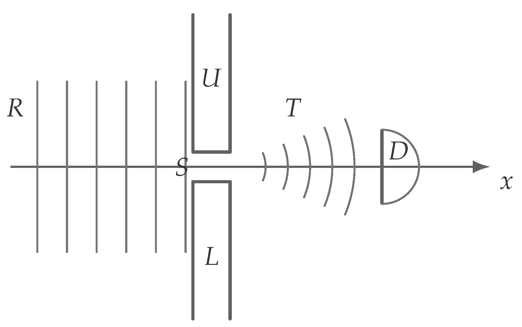
Figure 2.
The double slit experiment (barrier with two slits , screen )
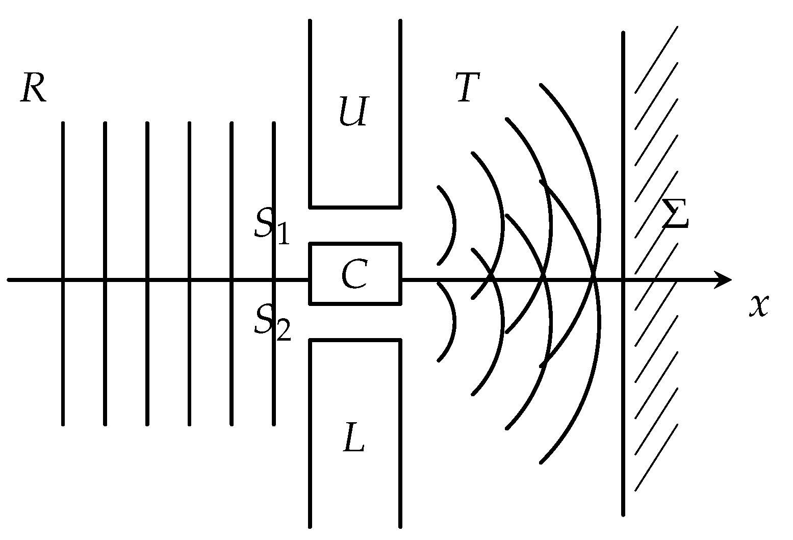
Disclaimer/Publisher’s Note: The statements, opinions and data contained in all publications are solely those of the individual author(s) and contributor(s) and not of MDPI and/or the editor(s). MDPI and/or the editor(s) disclaim responsibility for any injury to people or property resulting from any ideas, methods, instructions or products referred to in the content. |
© 2026 by the authors. Licensee MDPI, Basel, Switzerland. This article is an open access article distributed under the terms and conditions of the Creative Commons Attribution (CC BY) license (http://creativecommons.org/licenses/by/4.0/).
Copyright: This open access article is published under a Creative Commons CC BY 4.0 license, which permit the free download, distribution, and reuse, provided that the author and preprint are cited in any reuse.