

Submitted:
19 May 2026
Posted:
21 May 2026
You are already at the latest version
Abstract
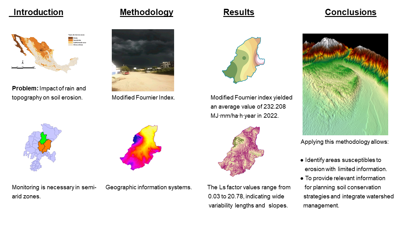
Water erosion is a critical degradation process that reduces fertility and agricultural sustainability, especially in semi-arid regions. The Universal Soil Loss Equation (USLE) allows for the quantification of this phenomenon using factors such as rainfall erosivity (R) and topography (length-slope, LS). In this study, both factors were estimated and analyzed in the Cañitas sub-basin, located in the semi-desert area of the state of Zaca-tecas, Mexico, characterized by irregular precipitation and limited data availability. The objective of this study is to estimate and analyze the R factor and LS factor to evaluate their influence on soil water erosion processes. Records from five meteorological stations (1986–2022) were used, along with the Modified Fournier Index (MFI) and Geographic Information Systems (GIS) tools, generating spatial maps of rainfall erosivity and to-pography. An average R factor of 240.608 MJ∙mm/ha∙h∙year was estimated, consistent with the values obtained using the MFI. The LS factor shows that the northwestern area of the study zone has the most extensive and steepest slopes (up to 20.78). This study provides useful information for understanding soil erosion processes, which can serve as a reference for planning conservation actions and managing watersheds in semi-arid areas with high climatic variability.
Keywords:
water erosion
; USLE
; R factor
; Modified Fournier Index
; LS factor
1. Introduction
One of the main environmental problems globally is soil erosion [1], due to its economic and social impact [2]. Loss of biodiversity, soil degradation, nutrient loss, and water and soil pollution are negative impacts of erosion. In 2018, the International Resolution on Soil and Water Conservation established that “global average soil erosion is estimated at between 12 and 15 t/ha/year” (FAO, 2018), meaning that, globally, the Earth’s land surface loses between 0.90 and 0.95 mm of soil annually.
The economic, social, and ecological impacts, which affect fertility, biodiversity, and water quality, have made soil erosion one of the main environmental problems, given its impact on fertility, biodiversity, and water quality. Precipitation, topography, and land use are fundamental factors in water erosion, which also exhibits high spatial and temporal variability. In this context, the integration of models such as USLE/RUSLE with geospatial tools has allowed progress in identifying critical areas; however, limitations persist in the detailed representation of these factors, especially in semi-arid regions with limited data. In particular, understanding the spatial distribution of the R factor and the heterogeneity of the LS factor remains a significant challenge for adequately interpreting erosive processes under conditions of climatic variability.
Aiello et al. in 2015 used a 20m digital elevation model (DEM) and the Desmet & Govers model, in southern Italy found that slopes greater than 15–20% increase erosion up to 10 times, with topographical factor being the main geomorphological control [3]. Using the RUSLE method and GIS, Tahiri, M., et al. in 2015 identified LS as one of the fundamental factors in the erosion process [4]. In the next year Panagos et al. using high-precision precipitation data, the R-value in Europe was analyzed using the RUSLE method, revealing high variability and elevated values associated with extreme events in the Mediterranean region. [5]. Panagos et al. using the GAM statistical model and the RUSLE method, found that erosivity is concentrated in autumn and winter, with a clear relationship between rainfall intensity and the spatial distribution of the erosivity factor [5]. In Rwanda in 2016, Karamage et al. used the USLE method, GIS, and remote sensing, finding that water erosion is very severe in Rwanda, concentrated in agricultural areas with steep slopes [6]. That same year, Gelagay, H. S. and Minale, A. S. used RUSLE, GIS and remote sensing, finding severe erosion in the Koga basin, related to topography, rainfall and intensive agricultural use [7]. In 2017 Panos Panagos, in collaboration with dozens of researchers, collaborated on a R factor global study using high-density climate databases, concluding that rainfall erosivity is highly variable in space and time, concentrating in the tropics and at specific seasons [8]. In the same year, Ahmed Benchettouh et al. assessed erosion risk using the integration of RUSLE and GIS, concluding that it is a powerful tool for diagnosing erosion and prioritizing areas for ecological restoration [9]. W.M. Navarro et al. analyzed in 2021 erosivity and its trend in Juliaca, calculating R using USLE and the Mann-Kendall method. They concluded that rainfall erosivity in Juliaca is high and variable, directly linked to annual precipitation, with no clear trend during the evaluated period, but with a potentially significant impact on soil erosion [10]. Next year Castro Villarreal et al. they used USLE and GIS methods to estimate soil loss in the Estibaná River sub-basin, comparing different types of vegetation cover and their effects, as well as agricultural management practices. Concluding that erosion in the Estibaná River sub-basin is a serious problem caused mainly by intense rainfall and rugged topography [12]. Ares and Entrantes, in that same year, conducted a study using the USLE equation, demonstrating the spatial and temporal interactions between different factors (precipitation, slope, soil, crops, management) [13]. At the same time Ricardo-Calzadilla et al. using local precipitation data (20 years), soil and topographic factors were estimated using the RUSLE method, validating indices such as rainfall erosivity, and employing the Modified Fournier Index to estimate erosion risk in the Los Palacios River sub-basin (Cuba). This reflected the spatial and temporal interactions between natural factors (rainfall, slope, soil) and anthropogenic factors (crops, management), where rainfall exhibits very high erosive aggressiveness [14]. In 2023 Bouayad et al. analyzed a basin in northwestern Morocco using GIS, DEM, and RUSLE, identifying risk areas and highlighting the LS and R factors importance of the RUSLE equation as the most relevant factors in the spatial variability of erosion [15]. In China, in 2024 the authors Li et al. applied the improved USLE equation methodology with global climatic, soil, topographic, and satellite data from 1992–2015, analyzing temporal trends and regional variations. They also validated the results by comparing them with previous global studies, concluding that global potential water erosion is highly sensitive to precipitation and changes in land cover [16]. The study by Gvozdenovich et al. provides a robust application of the USLE integrated with GIS to assess soil loss and its economic impact in an agricultural watershed, highlighting the effectiveness of conservation practices. Critical areas associated with slope and position in the landscape are identified [17]. The USLE/RUSLE methods, along with GIS and remote sensing, have enabled various studies worldwide (see Table 1) to demonstrate that heavy rainfall, topography, and land use are important factors in the erosion process. Water erosion has been shown to increase significantly with heavy rainfall and steep slopes, exhibiting marked spatial and temporal variability. This allows for the identification of risk zones and facilitates soil management and watershed planning. Previous studies demonstrate that topography and climate change significantly affect water erosion. This study contributes to the spatial accuracy of the R factor and demonstrates that the topographic LS factor exhibits a marked spatial heterogeneity associated with the influence of relief on water erosion. These results provide information for planning soil conservation strategies and integrated watershed management in semi-arid zones.
2. Materials and Methods
2.1. Study Area
The study area is located in the Cañitas Sub-basin, situated between the geographic coordinates -102°4’49.888564’’ longitude and 23°27’47.102213’’ latitude, within the Fresnillo-Yesca Basin, in the State of Zacatecas, Mexico. This region is located in a semi-desert zone, characterized by high-intensity rainfall over short periods, high hydroclimatic variability, and erosivity associated with high-intensity rainfall events [19].
The Cañitas sub-basin shares with several international studies the predominant influence of the R and LS factors on the dynamics of water erosion; however, it is distinguished by its semi-arid condition, limited data availability, and high climatic variability, which modifies the erosion generation mechanisms. Unlike tropical or temperate regions, where erosion is more constant, in Cañitas it is associated with intense but sporadic rainfall events. Furthermore, the use of different techniques for validating the R factor represents a significant contribution compared to studies lacking methodological rigor. The Cañitas Sub-basin (Figure 1) has an area of 4949.22 km² and a perimeter of 428.12 km (SIATL, 2025). Within the sub-basin, different land uses are observed (agricultural, land-use change, limited vegetation) associated with soil degradation processes. The Cañitas sub-basin contributes to surface runoff and the recharge of local aquifers, which is fundamental for the sustainable management of water resources in the northern part of the state of Zacatecas [24]. The analysis of the R (rainfall erosivity) and LS (topography) factors in the Cañitas sub-basin is fundamental to understanding the mechanisms that control water erosion in semi-arid environments characterized by high climatic variability, with rainfall concentrated between June and September. This favors short-duration, high-kinetic-energy erosion events. The R factor quantifies the energy and intensity of precipitation, while the LS factor shows the influence of topography on the erosion process. Evaluating both factors allow for identifying the spatial distribution of erosion risk and distinguishing areas where climatic or topographic effects predominate. Furthermore, this approach helps reduce uncertainty in erosion estimation using the USLE (United States of Local Erosion), particularly in contexts with limited information, thus strengthening the analysis of the erosion process at a local scale.
The aforementioned conditions and the physical properties of the soil make the Cañitas sub-basin a site of interest for evaluating water erosion and the potential impacts of climate change on soil loss [25].
Table 2 shows the general characteristics of the five weather stations analyzed over a period of more than 30 years.
This research aims to determine and evaluate the R factor and LS factor in the Cañitas Sub-basin, located in the Fresnillo-Yesca Basin within the semi-arid region of the State of Zacatecas, Mexico. GIS tools based on the Modified Fournier Index (MFI) were applied, enabling a spatial assessment of rainfall erosivity and topography in the study area.
This study provides new evidence on the spatial distribution of rainfall erosivity and the topographic influence on soil erosion in a semi-arid watershed in northern Zacatecas State, Mexico. It demonstrates the applicability of the Modified Fournier Index combined with GIS techniques in data-scarce environments.
2.2. Universal Soil Loss Equation
The Universal Soil Loss Equation (USLE) is a mathematical model that calculates water erosion of soil [26], based on factors given by Equation (1) [27].
where: A is the annual average soil erosion R is rainfall erosivity (MJ∙mm/ha∙h∙year), K is soil erodibility ( L is slope length (dimensionless), S is slope grade (dimensionless), C is crop and crop management (dimensionless), and P is soil management practices (dimensionless) [28].
2.3. Modified Fournier Index (MFI)
The index of maximum intensity in 30 minutes (EI_30) represents the result of the kinetic energy from the impact of raindrops on the soil multiplied by the maximum continuous intensity of precipitation over a 30-minute rainfall period. Fournier, in 1960, calculated the precipitation coefficient () to estimate erosivity [29]. Lombardi Neto and Moldenhauer (1992) established an equation between precipitation and erosivity using the Fournier Index (FI), where EI_30 and the precipitation coefficient are represented. This allows for the calculation of erosivity [30].
The R factor, called rainfall erosivity or soil erosivity, is a function of the kinetic energy and intensity of precipitation. The calculation is based on the climatic aggressiveness index or FI (Equation (2)), which is calculated using data from weather stations. The formula for the FI is obtained from Equation (2) [31].
where: FI is the Fournier Index, is the average precipitation of the rainiest month (mm), and P is the average annual precipitation (mm).
The MFI (Equation (3)) is obtained from the ratio of the sum of the squares of the monthly precipitation for a year to the total average annual precipitation [31].
where: MFI is the Modified Fournier Index, is the mean monthly precipitation (mm), and is the mean annual precipitation (mm).
In 2018 Benavidez et al. applied a correlation between the R factor and the MFI to readjust the model [32]. In 2016 Crettaz et al. stated that “The Modified Fournier Index by Arnoulds shows a high degree of fit with the R factor.” [31]. According to Jaya-Santillán in 2023, the equation for calculating the R factor is given by Equation (4) [33].
The calculation of the R-value is supported by ArcGIS software as a geospatial platform [34]. Weather stations are strategically located for the study, easing visualization, analysis of their distribution, and the generation of continuous surfaces across the study area. To calculate the R-value, data from five weather stations located near and within the study area were incorporated.
The inverse distance weighting (IDW) method was used for spatial interpolation of precipitation. This study includes five weather stations heterogeneously distributed across the study area, requiring an interpolation method that gives greater weight to values observed at points closer to the estimation location. In this regard, the IDW method is suitable, since it considers that the influence of data points decreases with distance, allowing the generation of a continuous surface that represents the spatial variability of precipitation. The result of the interpolation was a raster for each month of the year representing the precipitation across the entire sub-basin. The erosivity factor could then be calculated using the generated monthly rasters.
2.4. Topographic Factor LS
Slope length (L) and slope (S) are two fundamental elements in the USLE equation for calculating the LS factor in watershed studies, which includes the influence of topography on soil loss. [35].
Foster (1977) proposed Equations (5)-7 for L factor estimation.
where: L is the slope length (m), λ is the surface flow area (m²), F is the slope factor that defines m, m is the exponent influenced by the slope length and angle, and β is the slope angle.
In 2015, Panagos and Meusburger, building on the work of Desmet Gover (1996) and the emergence of GIS, proposed Equation (8) [5].
where: β Slope, A Flow accumulation, D Grid cell size (m), x Shape coefficient (x=1).
According to Renard et al. (1997), soil loss increases with slope length, hence the importance of the S factor [36].
The formula for obtaining the slope is derived from Equations (9) and (10) based on McCool et al. (1987) [36].
3. Results and Discussion
3.1. R Factor
Figure 2 shows the average results of the R factor at the five meteorological stations analyzed between 2000 and 2022, showing significant changes in precipitation.
The R-factor was calculated based on data from weather stations over the period 1986–2022 (National Meteorological Service).
Figure 2 shows that the stations exhibiting the highest R factor in 2020 and 2022 are located in the southwest of the sub-basin (32005) and in the southeast (32142). In 2010, the highest factor was found in the west (32001) and in the southeast (32142). In 2000, the highest R factor was found in the southwest (32005) and in the center of the sub-basin (32076).
The results indicate that the highest R factor recorded in 2022 reached 339.71 MJ∙mm/ha∙h∙year, concentrated in the southwest sector of the Cañitas sub-basin. This area shows greater susceptibility to water erosion due to the combination of high-intensity rainfall events that favor runoff generation. The spatial distribution of this maximum value suggests the influence of intense, short duration storms during the analyzed period, a typical behavior of semi-desert regions where storms occur in localized areas and with high kinetic energy (Figure 3).
The highest erosivity index in 2022 in the Cañitas sub-basin was obtained in the southwest (Figure 3).
The western part of the study area has the highest erosivity values, while the southern part has the lowest. Similarly, low erosivity values predominate in the central and eastern parts of the sub-basin, while average values are recorded in the north and center.
During the period 1986–2022, the rainfall erosivity values ranged from 219.088 MJ∙mm/ha∙h∙year in 1986 to 232.21 MJ∙mm/ha∙h∙year in 2022. The difference between the two years (13.12 MJ∙mm/ha∙h∙year) is relatively insignificant; however, some years show more marked variations, such as 1991, when erosivity reached considerably higher values than the historical average for the period studied (Figure 4).
The comparative analysis between the two methods applied shows that the R factor values obtained for 2022 are considerably similar. The method based on the MFI yielded an average value of 232.21 MJ∙mm/ha∙h∙year, while the geospatial processing method developed in ArcGIS yielded a value of 240.608 MJ∙mm/ha∙h∙year. The difference between the two results has a relative error of 3.49%, which demonstrates methodologically consistency and reinforces the reliability of the obtained values.
The closeness of the obtained values indicates that, even though both methods are based on different principles, they converge on a consistent representation of the erosive potential of precipitation, demonstrating that the estimation of the R factor is not affected by the different methodologies, thus strengthening the validity of the results (Table 3) [37]
In 1990 and 2010, the eastern part of the sub-basin had an R index of 941.89 and 678.04 MJ∙mm/ha∙h∙year, respectively. In 2018, the southern part had an R index of 608.92 MJ∙mm/ha∙h∙year; in all cases, the index was classified as high. The R index decreased throughout the basin due to the decline in precipitation.
3.2. LS Factor
The results of the LS factor (Figure 5) indicate that the northwest part has a topography with extensive lengths and steeper slopes, making it more prone to erosion.
Figure 5 and Figure 6 show significant spatial differences in the influence of topography within the Cañitas sub-basin. The LS values range from 0.03 to 20.78, indicating wide variability in lengths and slopes.
The northwest zone is characterized primarily by steep slopes and long hillsides, where surface runoff acquires greater energy and transport capacity, creating critical areas with erosion potential, especially during heavy rainfall. The eastern part of the sub-basin exhibits a low to moderate topographic intensity factor (0.94–3.77). Conversely, most of the sub-basin presents very low LS values (≤ 1), corresponding to gentle terrain with short slopes and relatively flat areas.
Table 4 shows the classification of the LS factor values [37].
The results show that potential erosion is conditioned by the R and LS factors, with the R factor remaining stable throughout the year, except during periods of intense rainfall. This analysis provides valuable information for the delimitation of priority conservation areas, decision-making, and the calibration of erosion models at a regional scale.
4. Discussion
The study revealed a decrease in the R factor related to reduced precipitation in the study area, with greater susceptibility in the southwest sector during intense rainfall events, while the rest of the Cañitas Sub-basin maintains a moderate level of erosivity. The LS factor showed marked spatial heterogeneity, identifying the northwest as the area with the greatest erosive potential due to its steep slopes and extensive hillsides. The rest of the Cañitas Sub-basin presents low LS values associated with gentle topography. These results allowed for the identification of two critical erosion areas controlled by distinct factors: rainfall erosivity and topography. Furthermore, the MFI was tested as a reliable alternative for calculating rainfall erosivity in semi-arid regions with limited data. This provides important information for planning soil conservation strategies and integrated watershed management in northern Zacatecas State, Mexico, such as agricultural terraces, living barriers, storage dams, and small dams, among others.
5. Conclusions
The analysis shows a decreasing trend in the R factor over the last few decades, from 607.91 MJ∙mm/ha∙h∙year in 1991 to 165.32 MJ∙mm/ha∙h∙year in 2019, which coincides with a reduction in regional precipitation. However, the southwest of the Cañitas sub-basin remains at moderate risk of water erosion during periods of heavy rainfall. Therefore, the R index is classified as moderate.
On the other hand, the LS factor results show marked spatial heterogeneity within the sub-basin. The northwest region has the most extensive slopes and the steepest gradients (LS up to 20.78), where surface runoff generates greater energy and transport capacity, creating critical areas of erosive potential. Conversely, most of the sub-basin area has low values (LS ≤ 1), associated with gentle relief and small slopes, where the topography has a minimal impact on erosion.
The analysis of the R and LS factors shows that the R factor in the southwest area indicates a greater tendency toward erosion, while the LS factor indicates a higher probability of erosion by transport in the northwest area due to the local topography. This identifies two critical areas susceptible to erosion from different causes. This provides empirical validation of the MFI as an alternative method for estimating rainfall erosivity in semi-arid environments with limited pluviographic data, strengthening the regional calibration of the USLE/RUSLE model. This contribution helps improve the spatial accuracy of the R factor. The LS factor shows marked spatial heterogeneity within the sub-basin, associated with the influence of topography on water erosion.
The results suggest that the critical areas identified are more likely to experience accelerated erosion.
These findings support the planning of soil conservation strategies and integrated watershed management in semi-arid regions of northern Mexico, which can serve as a basis for formulating recommendations on land management and use aimed at soil conservation.
Author Contributions
Conceptualization, L.C.-P.; E.D.M.-V. and J.V.-M.; methodology, L.C.-P. and E.D.M.-V.; software, L.C.-P. and E.D.M.-V.; validation, J.V.-M., R.S.-A., V.I.R.-A. and C.F.B.-C.; formal analysis, E.D.M.-V. and J.V.-M.; investigation, L.C.-P. and E.D.M.-V.; data curation, L.C.-P. and E.D.M.-V.; writing—original draft preparation, L.C.-P. ; writing—review and editing, L.C.-P.; E.D.M.-V.; J.V.-M.; R.S.-A and V.I.R.-A; visualization, R.S.-A.; V.I.R.-A. and C.F.B.-C.; supervision, E.D.M.-V., J.V.-M., R.S.-A. and V.I.R.-A. All authors have read and agreed to the published version of the manuscript.
Funding
This research received no external funding.
Data Availability Statement
The original contributions presented in this study are included in the article. Further inquiries can be directed to the corresponding author(s).
Acknowledgments
The authors gratefully acknowledge the National Council for Humanities, Sciences and Technologies (CONAHCYT) of Mexico for the scholarship awarded to Master of Mathematics Lorena Ceballos Pérez to pursue doctoral studies and conduct this research.
Conflicts of interest
The authors declare no conflicts of interest.
Abbreviations
The following abbreviations are used in this manuscript:
| R | Rainfall erosivity factor |
| GIS | Geographic Information System |
| MFI | Modified Fournier Index |
| LS | Topographic Factor |
| USLE | Universal Soil Loss Equation |
| t/ha/year | Tons of soil per hectare |
| FAO | Food and Agriculture Organization of the United Nations |
| DEM | Digital Elevation Model |
| RUSLE | Revised Universal Soil Loss Equation |
| GAM | Generalized Additive Model |
| MCDA | Multiple Criteria Decision Analisys |
| Rm | Rainfall magnitude |
| SWAT | Soil and Water Assessment Tool |
| C | Crop and crop management |
| ArcGIS | Software as a geospatial platform |
| L | Slope length |
| S | Slope grade |
| SIATL | Environmental and Territorial Information System (Sistema de Información Ambiental y Territorial) |
| Maximum intensity in 30 minutes | |
| Precipitation coefficient | |
| FI | Fournier Index |
| IDW | Inverse Distance Weighting |
| MJ∙mm/ha∙h∙year | Megajoules per millimeter per hectare per hour per year |
References
- Inoue, N.; Hamanaka, A.; Shimada, H.; Sasaoka, T.; Matsui, K. Fundamental study on soil erosion assessment using the USLE method in the rehabilitation area of an Indonesian coal mine. Earth Sci. Res. 2015, 4, 61. [Google Scholar] [CrossRef]
- Phinzi, K.; Ngetar, N.S. The assessment of water-borne erosion at catchment level using GIS-based RUSLE and remote sensing: A review. Int. Soil. Water Conserv. Res. 2019, 7, 27–46. [Google Scholar] [CrossRef]
- Aiello, A.; Adamo, M.; Canora, F. Remote sensing and GIS to assess soil erosion with RUSLE3D and USPED at river basin scale in southern Italy. CATENA 2015, 131, 174–185. [Google Scholar] [CrossRef]
- Tahiri, M.; Tabyaoui, H.; Tahiri, A.; El Hadi, H.; El Hammichi, F.; Achab, M. Modelling Soil erosion and sedimentation in the Oued Haricha sub-basin (Tahaddart watershed, Western Rif, Morocco): risk assessment. J. Geosci. Environ. Prot. 2015, 4, 107–119. [Google Scholar] [CrossRef]
- Panagos, P.; Ballabio, C.; Borrelli; P. y Meusburger, K. Spatio-temporal analysis of pluvial erosivity and erisivity density in Greece. Catena 2016, 137, 161–172. [Google Scholar] [CrossRef]
- Karamage, F.; Zhang, C.; Ndayisaba, F.; Shao, H.; Kayiranga, A.; Fang, X.; Tian, G. Extent of cropland and the related risk of soil erosion in Rwanda. Sustainability 2016, 8, 609. [Google Scholar] [CrossRef]
- Gelagay, H.S.; Minale, A.S. Estimation of soil loss using GIS and remote sensing techniques: A case study of the Koga River Basin, northwestern Ethiopia. Int. Res. Soil. Water Conserv. 2016, 4, 126–136. [Google Scholar] [CrossRef]
- Panagos, P.; Borrelli, P.; Meusburger, K.; Yu, B.; Klik, A.; Jae Lim, K.; Ballabio, C. Global assessment of rainfall erosivity based on high-temporal-resolution precipitation records. Sci. Rep. 2017, 7, 4175. [Google Scholar] [CrossRef]
- Benchettouh, A.; Kouri, L.; Jebari, S. Spatial estimation of soil erosion risk using RUSLE/GIS techniques and suggested conservation practices to reduce soil erosion in the Wadi Mina watershed (northwest Algeria). Arab. J. Geosci. 2017, 10, 79. [Google Scholar] [CrossRef]
- Calero, M. D.; Martínez, L. C.; Menjívar, F. J.C. Evaluación de modelos para estimar la erosividad de la Lluvia en el valle del Cauca, Colombia. Acta Agronómica 2021, 70, 198–210. [Google Scholar]
- Castro-Villarreal, J.A.; Cabrera-Rodríguez, J.A.; Villarreal-Núñez, J.E. Pérdida de suelo evaluada por el método USLE en la subcuenca del río Estibaná, Panama. Acta Agronómica 2022, 71, 369–376. [Google Scholar]
- Ares, M.G.; Entraigas, I. Effects of spatial and temporal heterogeneity on soil loss in an agricultural watershed. 2022. Available online: https://www.revistaecosistemas.net/index.php/ecosistemas/article/view/2298 (accessed on 10 January 2026).
- Ricardo-Calzadilla, M. P.; Gómez-Arias, A.; Cutie-Cansino, V. Erosividad de las lluvias en Finca Tierra Brava de la subcuenca (S1) Río Los Palacios. Ing. Agrícola 2022, 12, 4. [Google Scholar]
- Bouayad, F.E.; ELIdrysy, M.; Ouallali, A.; ELAmrani, M.; Courba, S.; Hahou, Y.; Benhachmi, M.K.; Spalevic, V.; Briak, H. ASSESSING SOIL EROSION DYNAMICS IN THE RMEL WATERSHED, NORTHERN MOROCCO BY USING THE RUSLE MODEL, GIS, AND REMOTE SENSING INTEGRATION. J. "Agric. For. 2023, 69. [Google Scholar] [CrossRef]
- Li, J.; Xiong, M.; Sun, R.; Chen, L. Temporal variability of global potential water erosion based on an improved USLE model. Int. Soil. Water Conserv. Res. 2024, 12, 1–12. [Google Scholar] [CrossRef]
- Gvozdenovich, J. J.; Saluzzio, M. F.; Crettaz, M. E.; Folmer, M. A.; Gregorutti, V. C.; Dorelo, M. P. B.; Gaitan, J. J. Environmental and economic impact of soil and water conservation through the systematization of the La Ensenada Stream basin. Science, Teaching and Technology Supplement. 2025, 15. Available online: https://pcient.uner.edu.ar/index.php/Scdyt/article/view/2203 (accessed on 10 January 2026).
- Aguirre-Salado, C.A.; Miranda-Aragón, L.; Pompa-García, M.; Reyes-Hernández, H.; Soubervielle-Montalvo, C.; Flores-Cano, J.A.; Méndez-Cortés, H. Improving Identification of Areas for Ecological Restoration for Conservation by Integrating USLE and MCDA in a GIS-Environment: A Pilot Study in a Priority Region Northern Mexico. ISPRS Int. J. Geo-Inf. 2017, 6, 262. [Google Scholar] [CrossRef]
- Gaubi, I.; Chaabani, A.; Ben Mammou, A.; Hamza, M.H. GIS-based prediction of soil erosion using the Revised Universal Soil Loss Equation (RUSLE) (Lebna River Basin, Cape Bon, Tunisia). Nat. Hazards 2017, 86, 219–239. [Google Scholar] [CrossRef]
- Yue, T.; Xie, Y.; Yin, S.; Yu, B.; Miao, C.; Wang, W. Effect of time resolution of rainfall measurements on the erosivity factor in the USLE in China. Int. Soil. Water Conserv. Res. 2020, 8, 373–382. [Google Scholar] [CrossRef]
- Fiener, P.; Dostál, T.; Krása, J.; Schmaltz, E.; Strauss, P.; Wilken, F. Operational USLE-Based Modelling of Soil Erosion in Czech Republic, Austria, and Bavaria—Differences in Model Adaptation, Parametrization, and Data Availability. Appl. Sci. 2020, 10, 3647. [Google Scholar] [CrossRef]
- Marcillo JLMy Triana, L.V. Riesgo de erosión del suelo en el cantón Mocache aplicando análisis multicriterio y sistemas de información geográfica. Rev. Geográfica De Chile Terra Aust. 2024, 60, 1. [Google Scholar]
- Santos, A.D. S.; Silva Júnior, J. F. D.; Santos, L. D. S.; Alencar Sobrinho, R. J.; Amorim, E. C.; Fernandes, G. S. T.; Jardim, A. M. D. R. F. Identification of Priority Areas for the Control of Soil Erosion and the Influence of Terrain Factors Using RUSLE and GIS in the Caeté River Basin, Brazilian Amazon. Earth 2025, 6, 35. [Google Scholar] [CrossRef]
- Lozano-Rivas, W.A. Clima, hidrología meteorología: Para ciencias ambientales e ingeniería; Universidad Piloto de Colombia, 2018. [Google Scholar]
- Panagos, P.; Ballabio, C.; Borrelli, P.; Meusburger, K.; Klik, A.; Rousseva, S.; Tadić, M.P.; Michaelides, S.; Hrabalíková, M.; Olsen, P.; et al. Rainfall erosivity in Europe. Sci. Total. Environ. 2015, 511, 801–814. [Google Scholar] [CrossRef]
- Loaiza, S.; Silva, M.A.D. Evaluación del potencial de mitigación de las estrategias de adaptación implementadas en los Territories Sostenibles Adaptados al Clima (TeSAC), 2018. Available online: https://hdl.handle.net/10568/93413 (accessed on 10 January 2026).
- Valdivia-Martínez, O.; Peña-Uribe, G.D. J.; Rufino-Rodríguez, F.; Torres-González, J. A.; Meraz-Jiménez, A. D. J.; López-Santos, A. Ajuste de la Ecuación Universal de Pérdida de Suelo en parcelas de escurrimiento ubicadas en una región del centro de México. Terra Latinoam. 2022, 40. [Google Scholar] [CrossRef]
- Alewell, C.; Borrelli, P.; Meusburger, K.; Panagos, P. Using the USLE: Chances, challenges and limitations of soil erosion modelling. Int. Soil. Water Conserv. Res. 2019, 7, 203–225. [Google Scholar] [CrossRef]
- Wischmeier, W. H.; Smith, D. D. Predicting losses from rainfall erosion: a guide for conservation planning (No. 537); Department of Agriculture, Science and Educational Administration, 1978. [Google Scholar]
- Behrends Kraemer, F.; Chagas, C. I.; Ibañez, L.; Carfagno, P.; Vangeli, S. Análisis de la erosividad de las lluvias para el partido de San Pedro (Bs. As.). Cienc. Del Suelo 2018, 36, 124–137. [Google Scholar]
- Crettaz, E.; Gvozdenovich, J.; Saluzzio, M. CALCULO DEL FACTOR R DE LA USLE A TRAVES DEL INDICE MODIFICADO DE FOURNIER. INTA Paraná. 2016. Available online: https://www.researchgate.net/profile/Jj-Gvozdenovich/publication/321058206_CALCULO_DEL_FACTOR_R_DE_LA_USLE_A_TRAVES_DEL_INDICE_MODIFICADO_DE_FOURNIER/links/5a0b06720f7e9b0cc025169f/CALCULO-DEL-FACTOR-R-DE-LA-USLE-A-TRAVES-DEL-INDICE-MODIFICADO-DE-FOURNIER.pdf (accessed on 8 April 2025).
- Benavidez, R.; Jackson, B.; Maxwell, D.; Norton, K. A review of the (Revised) Universal Soil Loss Equation ((R)USLE): with a view to increasing its global applicability and improving soil loss estimates. Hydrol. Earth Syst. Sci. 2018, 22, 6059–6086. [Google Scholar] [CrossRef]
- Jaya-Santillán, J. Altos niveles de erosión hídrica en una microcuenca tropical calculados mediante el modelo USLE. FIGEMPA Investig. Y Desarro. 2023, 15, 26–39. [Google Scholar] [CrossRef]
- Ghosh, A.; Rakshit, S.; Tikle, S.; Das, S.; Chatterjee, U.; Pande, C.B.; Alataway, A.; Al-Othman, A.A.; Dewidar, A.Z.; Mattar, M.A. Integration of GIS and Remote Sensing with RUSLE Model for Estimation of Soil Erosion. Land 2022, 12, 116. [Google Scholar] [CrossRef]
- Anampa, M.H. A.; Soldevilla, M. Y. E.; Araujo, V. G. S. Estimation of the topographic factor LS (RUSLE) using geographic information systems: The Ichu sub-basin case, Huancavelica, Peru. Polo Del Conoc. Rev. Científica-Prof. 2021, 6, 66–81. Available online: https:// (accessed on 6 June 2025).
- Michalopoulou, M.; Depountis, N.; Nikolakopoulos, K.; Boumpoulis, V. The Significance of Digital Elevation Models in the Calculation of LS Factor and Soil Erosion. Land 2022, 11, 1592. [Google Scholar] [CrossRef]
- Rengifo-Rengifo, I. Y.; Muñoz-Gómez, F. A.; Toro-Trochez, O. A. USLE model for estimating water erosion in seven municipalities of the Colombian Andean region. Biotechnol. Agric. Agro-Ind. Sect. 2022, 20, 29–44. [Google Scholar]
Figure 1.
Location of the Cañitas sub-basin and the five meteorological stations analyzed.
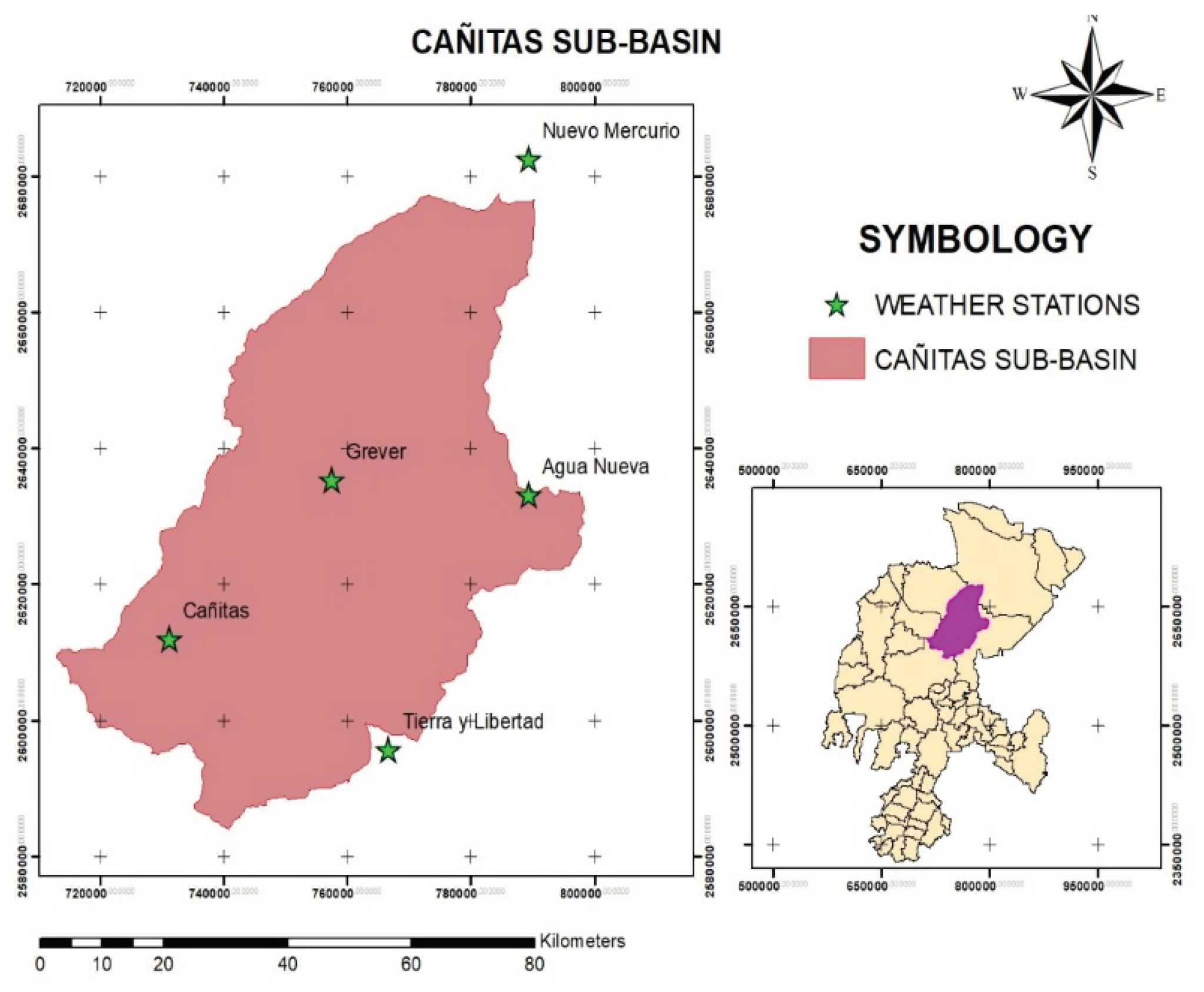
Figure 2.
Average of the R factor where significant changes in precipitation are shown.
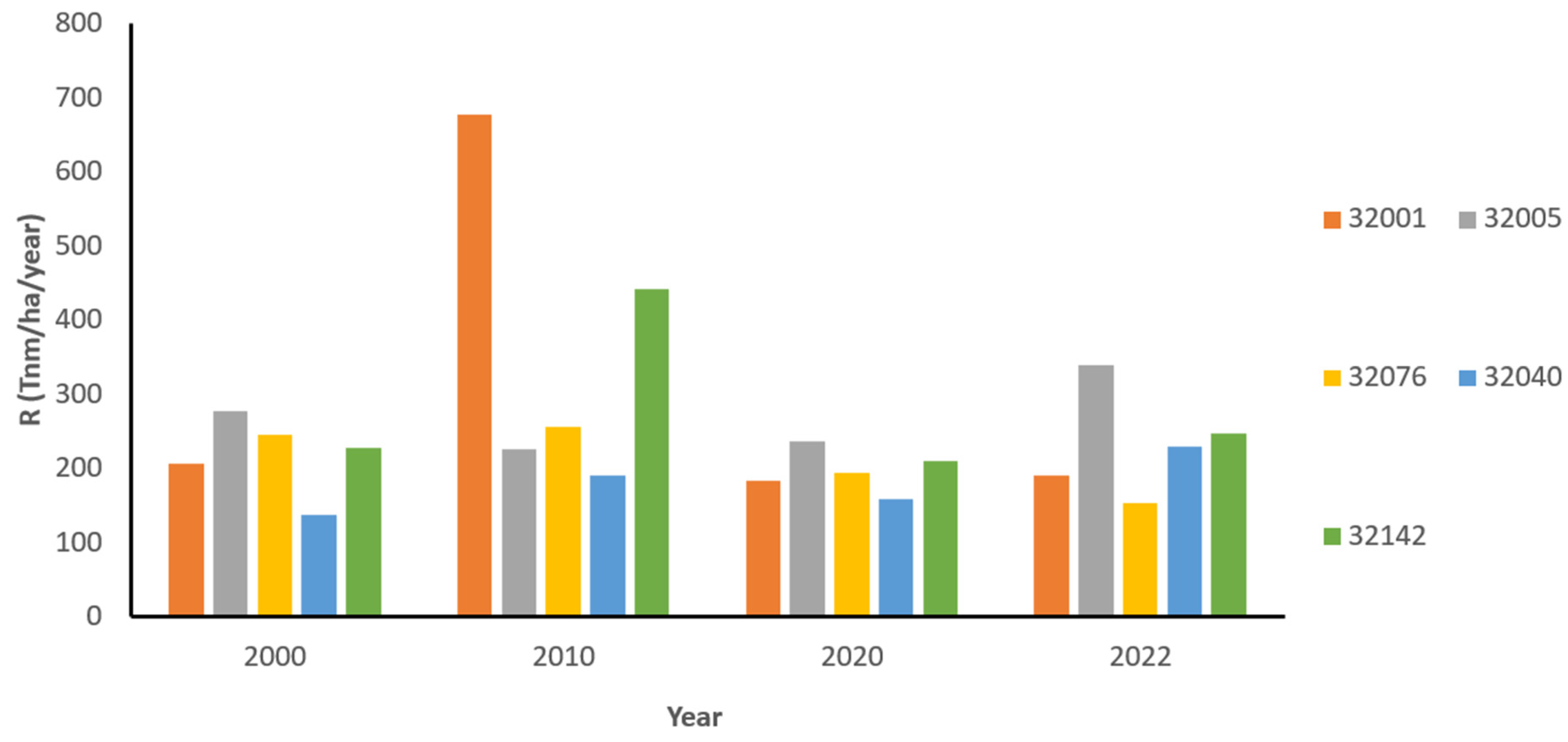
Figure 3.
Erosivity factor map of the Cañitas sub-basin (2022) shows the southwestern zone with the highest erosivity index.
Figure 3.
Erosivity factor map of the Cañitas sub-basin (2022) shows the southwestern zone with the highest erosivity index.
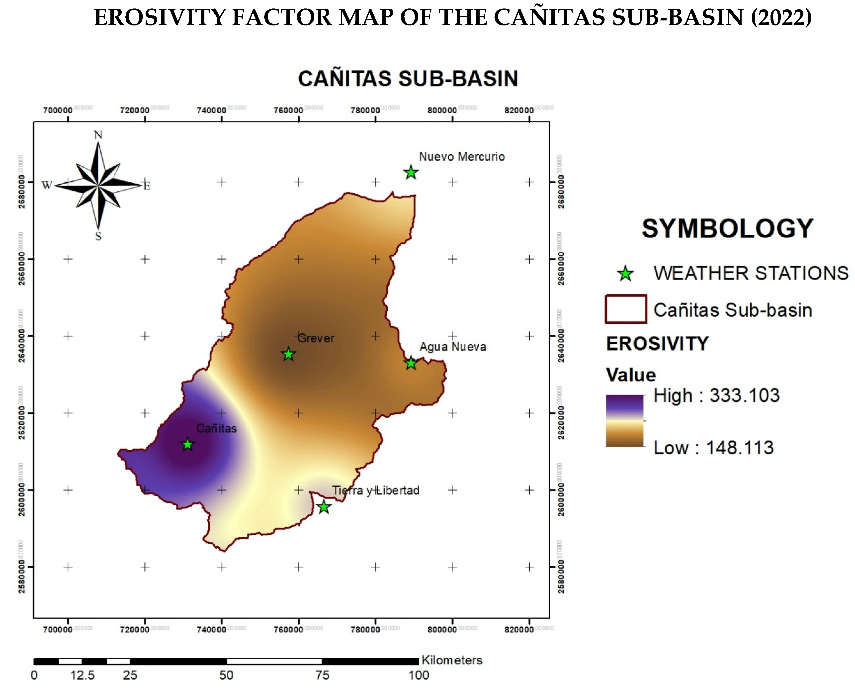
Figure 4.
Average R factor for the period 1986-2022, where the variability of precipitation can be observed.
Figure 4.
Average R factor for the period 1986-2022, where the variability of precipitation can be observed.
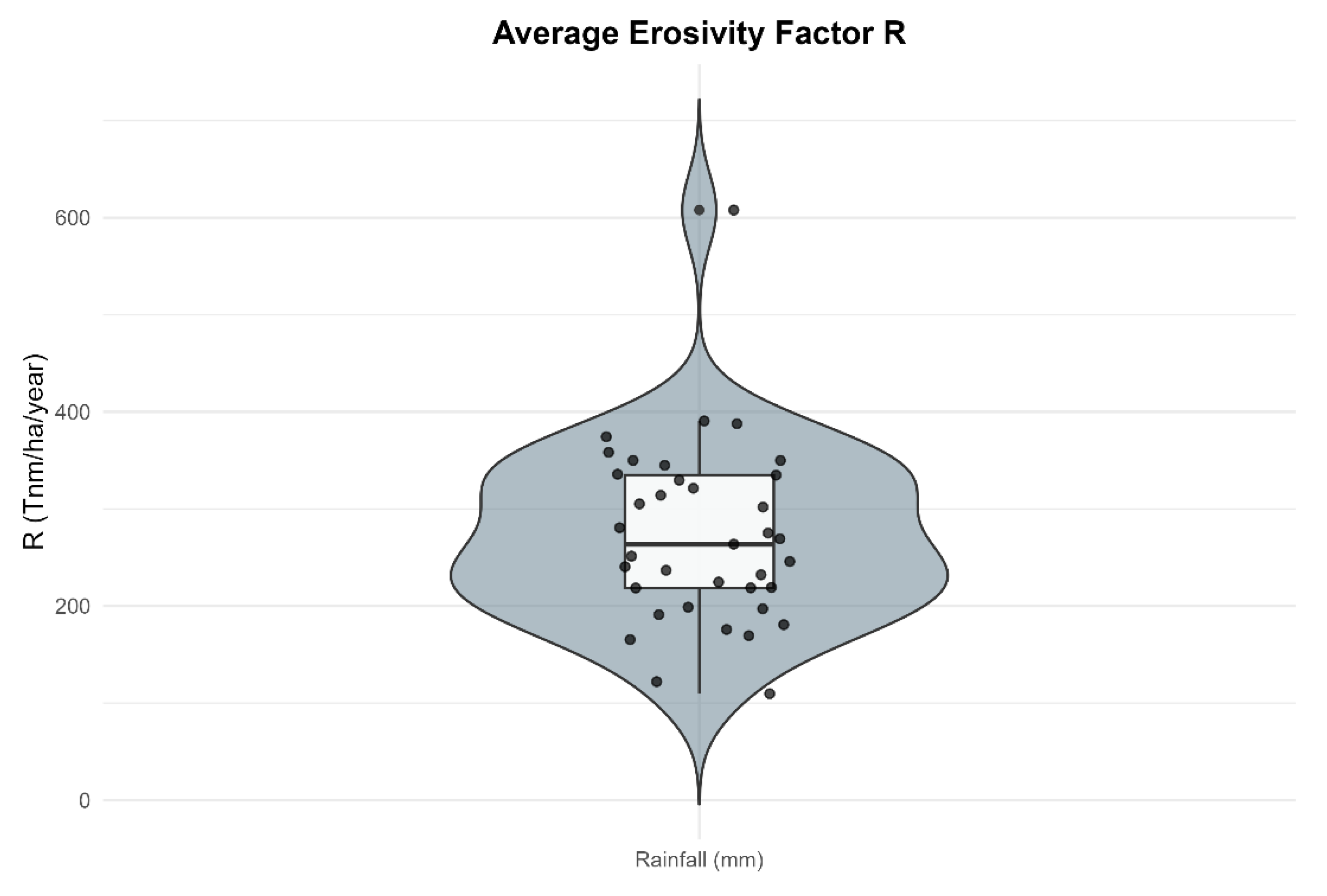
Figure 5.
The LS factor shows the northwest part with a topography with extensive lengths and steeper slopes.
Figure 5.
The LS factor shows the northwest part with a topography with extensive lengths and steeper slopes.
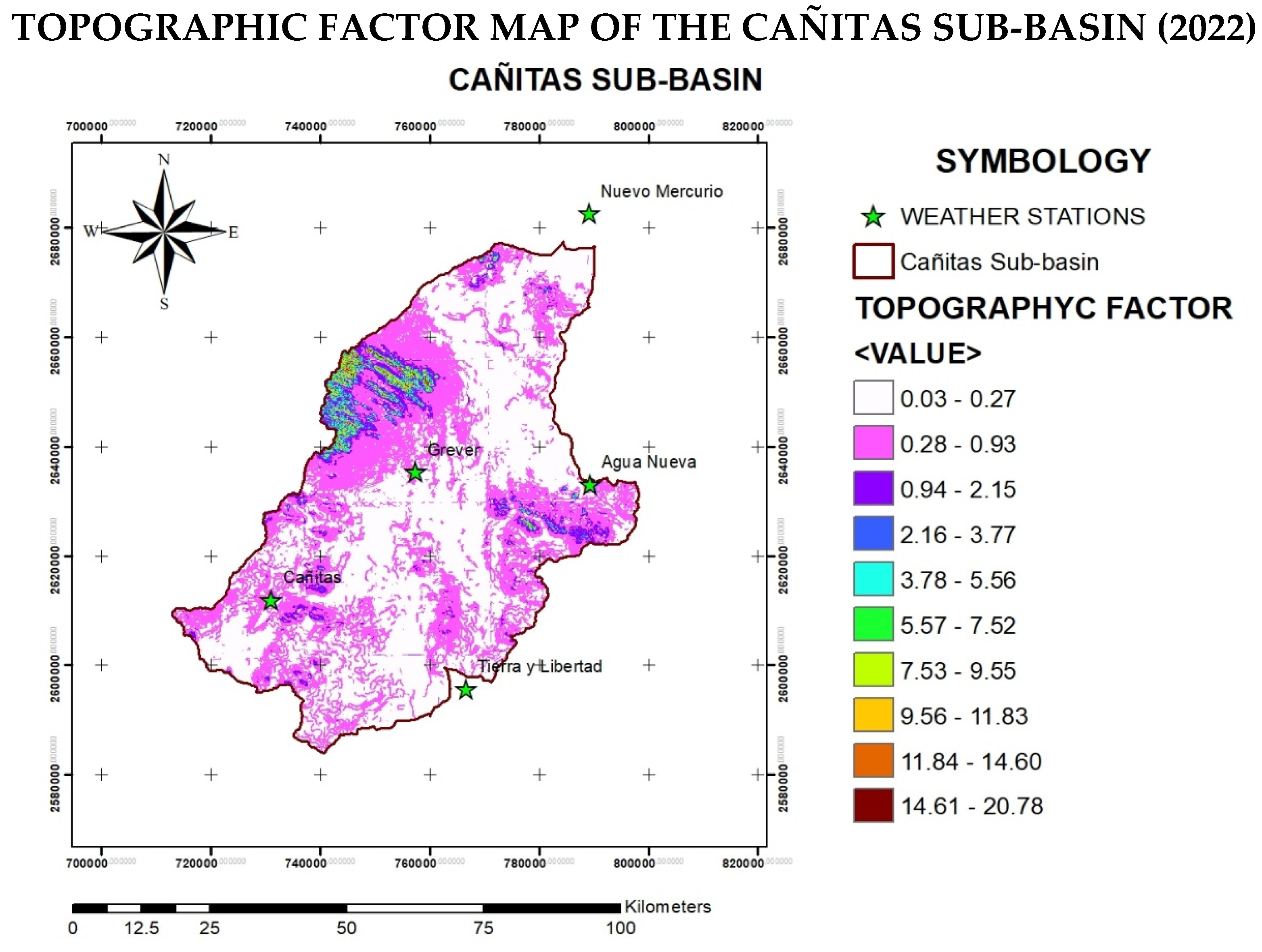
Figure 6.
Approach to the northwest zone of the LS factor with extensive lengths and steeper slopes.
Figure 6.
Approach to the northwest zone of the LS factor with extensive lengths and steeper slopes.
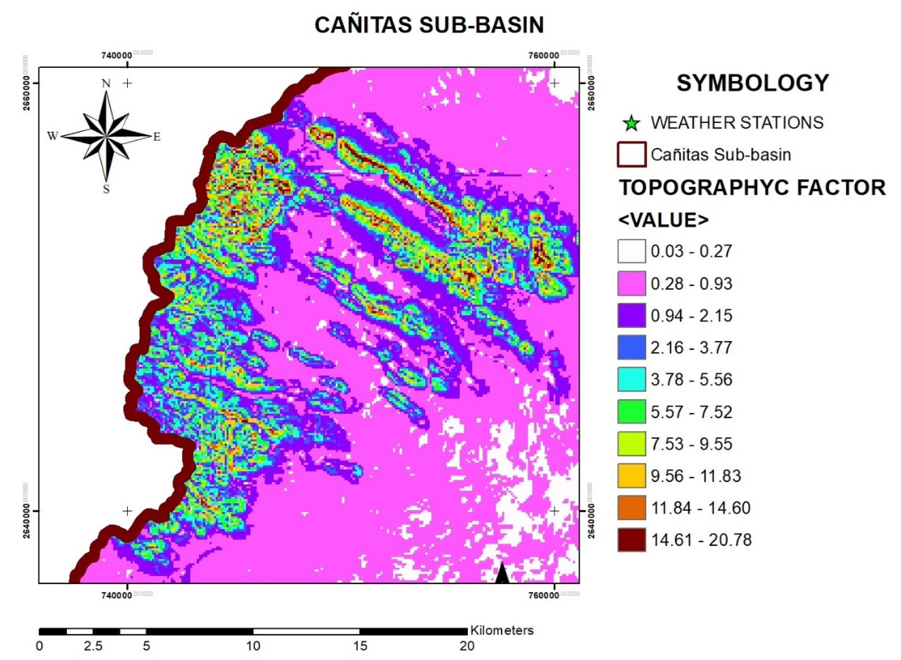

Table 1.
Some of the studies carried out in the period 2015-2025.
| Author/ Year |
Country/ Region |
Methodology | Main focus |
Main findings | Limitations | Comparison with the present article |
|---|---|---|---|---|---|---|
| Tahiri et al. (2015) | Morocco |
RUSLE+GIS |
Spatial analysis. | LS as a fundamental factor. | Without temporal analysis of R factor. | A temporal analysis of the R factor is included. |
| Panagos et al. (2016) | Greece |
RUSLE+DEM high resolution + GAM |
Spatiotemporal erosivity (R factor). | High spatial and temporal variability. | Dependence on high-resolution pluviographic data. Approach with Mediterranean dictions. |
Analysis with limited rainfall data. Semi-arid zone. |
| Karamage et al. (2016) | Rwanda |
RUSLE+GIS |
Erosion assessment. | High erosion in sloping agricultural areas. |
Tropical context. | Semi-arid zone. |
| Gelagay et el. (2016) | Ethiopia |
RUSLE+DEM (30 m) |
Critical erosion zones. | Identification of vulnerable areas. | Without methodological validation. | Validate alternative methods. |
| Panagos et al. (2017) | Global | RUSLE+ climatological data | Global R factor. | High spatial and temporal variability. | Global scale without local detail. | Detailed local análisis. |
| Benchettouh et al. (2017) | Algeria |
RUSLE+GIS |
Risk of erosion. | A useful tool for planning. | Without validation of the R factor or long time series. | Validation of the R factor, using series 1986-2022. |
| Navarro et al. (2021) | Perú | USLE + Mann-Kendall |
R Factor |
High erosivity and decreasing erosivity trend | Short series (2013-2017); not calculated LS | Cañitas uses a long series, including LS and methodological validation |
| Calero et al. (2021) | Colombia |
Empirical models of R |
Erosivity assessment |
Significant differences between methods |
Data dependency; does not include LS. |
Cañitas validates R (IMF vs GIS) and includes LS in semi-arid zone |
| Aguirre-Salado et al. (2017) | Mexico |
RUSLE+SWAT+HIT |
Agricultural basins. | Integration of hydrological models. | Not validated in semi-arid zones. | Focused on semi-arid zones. |
| Gaubi et al. (2017) | Tunisia |
RUSLE |
R and LS factors. | Interaction between factors in the Mediterranean Basin. | Without methodological comparison. | MFI vs GIS is compared. |
| Yue et al. (2020) | China | Rainfall Temporal Resolution Analysis + USLE (R factor) | R factor accuracy. | Erosivity decreases when using low temporal resolution data; errors increase >15 min. | Dependence on high-resolution data; methodological approach. | Cañitas uses limited data but validates R with alternative methods. |
| Fiener et al. (2020) | Europe (Czech Republic, Germany, Austria) |
USLE/RUSLE comparative + SIG |
Comparison of model implementations. | Differences of up to 75% in erosion estimates depending on implementation. Even greater variability at the plot scale. |
Lack of standardization between countries. |
Cañitas provides methodological validation of the R and analysis under semi-arid conditions, reducing local uncertainty. |
| Castro Villarreal et al. (2022) | Panama |
USLE+ plots +GIS |
Soil use | Influence of soil cover and management. | No methodological validation of the R factor. | Validation of R factor, analyzes R and LS factors. |
| Ares et al. (2022) | Argentina |
USLE (monthly scale) |
Spatio-temporal analysis. | Interaction of natural and anthropogenic factors. | Monthly scale. | Annual Scale. |
| Marcillo & Triana (2024) | Ecuador |
MCDA + GIS |
Risk zoning. | Identification of critical areas by slope and cover. | Subjectivity in weightings; no physical model or validation. | Cañitas uses USLE, a quantitative approach in R and LS. |
| Li et al. (2024) | China | USLE+DEM+GIS | Global trends. | High sensitivity to climate and land use. |
Global scale. |
Regional scale. |
| Santos et al. (2025) | Brazil |
RUSLE + GIS + MLR |
Identification of priority areas and geomorphometric control. | Predominantly low risk, with localized critical areas. Topographic factors explain much of the variability. Identification of key geomorphological variables (curvature, humidity index, etc.). |
The model partially explains the variability. Dependence on spatial data. Tropical regional focus. |
Cañitas delves into specific R and LS, including methodological validation (IMF vs GIS) and temporal analysis in a semi-arid zone. |
Table 2.
General characteristics of climatological stations (National Meteorological Service).
| Weather Station | Name | Basin | Municipality | Latitude | Longitude | Msnm | Years of Service |
|---|---|---|---|---|---|---|---|
| 32001 | Agua Nueva | Fresnillo-Yesca | Villa de Cos, Zac. | 23°46’58’’ | -102°09’37’’ | 1932 | 1964-2022 |
| 32005 | Cañitas de Felipe Pescador | Fresnillo-Yesca | Cañitas de Felipe Pescador | 23°36’08’’ | -102°44’02’’ | 2046 | 1941-2022 |
| 32040 | Nuevo Mercurio | Camacho-Gruñidora | Mazapil, Zac. | 24°13’38’’ | -102°09’09’’ | 1706 | 1969-2022 |
| 32076 | Col. Grever La Colorada | Fresnillo-Yesca | Villa de Cos, Zac. | 23°48’34’’ | -102°28’19’’ | 1950 | 1971-2023 |
| 32142 | Tierra y Libertad | Fresnillo-Yesca | Villa de Cos, Zac. | 23°27’00’’ | -102°23’32’’ | 2030 | 1982-2023 |
Table 3.
Classification of R Factor values.
| R Factor | R factor classification |
|---|---|
| 0-50 | Light |
| 50-500 | Moderate |
| 500-1000 | High |
| >1000 | Very high |
Table 4.
Classification of LS Factor.
| CLASS | LS factor classification | VALUE |
|---|---|---|
| 1 | < 1.5 | Very low |
| 2 | 1.6-3 | Low |
| 3 | 3-5 | Moderate |
| 4 | 5.1-7 | High |
| 5 | > 7 | Very high |
Disclaimer/Publisher’s Note: The statements, opinions and data contained in all publications are solely those of the individual author(s) and contributor(s) and not of MDPI and/or the editor(s). MDPI and/or the editor(s) disclaim responsibility for any injury to people or property resulting from any ideas, methods, instructions or products referred to in the content. |
© 2026 by the authors. Licensee MDPI, Basel, Switzerland. This article is an open access article distributed under the terms and conditions of the Creative Commons Attribution (CC BY) license (http://creativecommons.org/licenses/by/4.0/).
Copyright: This open access article is published under a Creative Commons CC BY 4.0 license, which permit the free download, distribution, and reuse, provided that the author and preprint are cited in any reuse.


