

Submitted:
15 May 2026
Posted:
18 May 2026
You are already at the latest version
Abstract
Using liquid hydrogen (LH2) in aviation creates a difficult design problem for cryogenic storage systems, especially in the early design stage. At that point, environmental, economic, and technical aspects need to be considered together. Here, a sustainability assessment framework is presented for LH2 aircraft storage tank configurations from a life-cycle perspective. The study includes 24 design alternatives. These are obtained by changing the material combinations of the main structural components, while the overall tank architecture is kept unchanged. The environmental and economic dimensions are assessed through Life Cycle Assessment (LCA) and Life Cycle Costing (LCC), whereas the technical dimension is represented by system mass. Since the relative importance of the criteria is usually not fixed at this stage, Unweighted TOPSIS (UW-TOPSIS) is first used to examine the alternatives under different weighting scenarios. The most competitive solutions are then re-evaluated by a standardised TOPSIS variant (vector-normalised weights, Z-standardised distances) with objective weighting methods. The results show that the configurations based entirely on Al2219-T8 for the main structural components remain top-ranked and more stable under the examined scenarios, whereas mixed-material configurations are more sensitive to changes in weighting assumptions. In this way, the exploratory stage is kept separate from the later weighting stage, where the weights are computed from the decision matrix of the reduced set. This is suitable for early aerospace design, where subjective preferences are often not yet available.
Keywords:
sustainability assessment
; hydrogen aviation
; liquid hydrogen storage tanks
; unweighted TOPSIS
; interval weights
; life cycle assessment
; life cycle costing
1. Introduction
Aviation must reduce its environmental burden if the broader climate targets of the Paris Agreement are to be met [1]. This requirement has renewed interest in zero-emission aircraft concepts. Among the available options, liquid hydrogen (LH2) is often discussed as a promising energy carrier because it does not emit carbon at the point of use and may support long-range flight. Still, the assessment of LH2-based aviation cannot stop at in-flight operation. Its overall performance depends on the whole chain, including hydrogen production, liquefaction, distribution, and the aircraft technologies needed to store and use it, especially cryogenic tanks and propulsion systems. Recent studies suggest that, even though LH2 may require more energy during flight, it can perform better than sustainable aviation fuels (SAFs) when the comparison is made on a life cycle basis [2]. This makes a system-level and life-cycle-based assessment necessary [3]. A similar perspective also appears in current European research programmes, including H2ELIOS, where fuel pathways and aircraft technologies are examined together in the broader effort toward climate-neutral aviation.
The literature on alternative aviation fuels points in the same direction. Several studies show that environmental gains cannot be judged only from in-flight emissions, because upstream production stages and supply-chain effects also contribute [4,5]. Even so, much of this work still focuses mainly on environmental performance. Economic and technical aspects, although also important in engineering design, are often treated more briefly or left outside the analysis. Some more recent studies have started to link environmental assessment with aircraft design and, in some cases, with economic considerations as well [6]. These studies make clear that a shift to fuels such as LH2 also affects aircraft layout and system design.
For LH2 cryogenic tanks, material selection and structural design are especially important. The main trade-off is usually between metallic and composite solutions [7]. Carbon fibre reinforced polymers (CFRPs), for example, are attractive because of their high strength-to-weight ratio and their potential to reduce mass [8]. At the same time, their production and end-of-life treatment may create environmental and economic burdens [9]. Their use in LH2 tank applications is also limited by practical concerns, including long-term durability, microcracking, permeability, and inspectability [7].
Related life cycle studies, many of them from the automotive field, show that hydrogen storage systems may contribute substantially to total environmental impacts and may involve nontrivial trade-offs in both energy use and cost [9,10]. Taken together, these results suggest two things. First, environmental and economic dimensions are still often analysed separately. Second, LH2 aviation systems need evaluation frameworks that can address several dimensions at the same time. In practice, LH2 storage is a multi-criteria problem, since environmental, economic, and technical criteria have to be considered together and may point in different directions. Similar situations also arise in other energy systems, where trade-offs have to be examined over the full life cycle [11].
For problems of this kind, multiple-criteria decision-making (MCDM) methods are a natural option. They have already been applied in aerospace design, including the authors’ earlier studies on aircraft structures, where environmental, economic, and technical criteria were analysed jointly and the effects of material choice, geometry, and joining strategy were examined in a systematic way [12,13]. In those studies, objective weighting methods were used so that criterion importance came from the data rather than from subjective judgement. Even so, the issue of weighting is still difficult, especially at an early design stage. At that point, stakeholder preferences are often not fixed, while the ranking of alternatives may still depend strongly on the chosen weights. Methods such as Unweighted TOPSIS (UW-TOPSIS) were proposed for this reason. They allow the analyst to work with weight intervals instead of fixed weights and therefore avoid prescribing criterion importance in advance [14,15].
In the specific case of LH2 storage systems, there are still few sustainability assessment studies that use MCDM while also treating uncertainty in criterion importance explicitly. The present study addresses that gap. It develops a decision framework for LH2 storage configurations and uses it to compare alternative designs while also examining how sensitive the ranking is to the weighting scheme. UW-TOPSIS is used first, in order to explore the design space without fixed weights. A standardised TOPSIS variant with data-driven weighting methods is then applied in the second stage to the reduced set of alternatives. In this way, the first stage reveals how much the ranking depends on the choice of weights, whereas the second stage derives the final weights directly from the reduced decision matrix. As a result, subjective weighting assumptions do not determine the final choice among the LH2 storage configurations studied here.
2. Technological Problem
This section examines the sustainability performance of liquid hydrogen (LH2) storage tank configurations for zero-emission aircraft. The analysis starts from a baseline design developed in the H2ELIOS project. The goal is to identify the configurations that perform best when environmental, economic, and technical criteria are considered together under different design priorities. The main difficulty at this stage is that the relative importance of these criteria is usually not agreed in advance. For that reason, the first part of the analysis applies Unweighted TOPSIS (UW-TOPSIS), so that the alternatives can be explored under admissible weight intervals. The alternatives that remain competitive are then re-examined by a standardised TOPSIS variant with objective weighting methods. This gives a more focused comparison of the candidate configurations.
2.1. Tank Configuration and Design Space
The LH2 tank considered here has fixed geometry and a fixed system layout. This reflects both the complexity of cryogenic tank design and the strict functional requirements that such systems must satisfy. Geometric variations are therefore outside the scope of the present analysis. The design space is restricted instead to material selection for four main structural parts: the outer tank, the inner tank, the outer supports, and the inner supports.
Figure 1.
(a) Outer tank configuration of the LH2 storage system, illustrating the complete external geometry of the assembly. (b) Sectional view showing the internal configuration.
Figure 1.
(a) Outer tank configuration of the LH2 storage system, illustrating the complete external geometry of the assembly. (b) Sectional view showing the internal configuration.
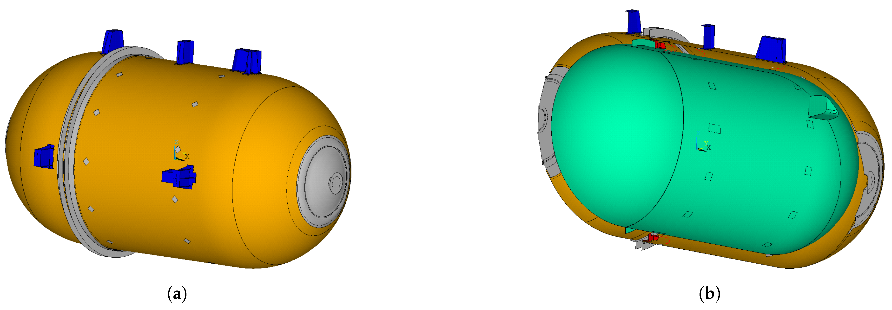
Under these assumptions, the feasible alternatives come from the different material combinations selected for the main structural components. This gives 24 configurations in total. Together, they cover all combinations of the available material options for the inner tank, outer tank, and support structures. These configurations constitute the set of decision alternatives considered in this study. Their main characteristics are listed in Table 1.
The candidate materials used to build these combinations are aluminium alloy Al2219-T8, stainless steel AISI 316L, and carbon fibre reinforced polymer (CFRP). For discussion purposes, the 24 alternatives can be arranged into six groups of four, depending on the outer-tank and inner-tank material pair, as shown in Table 2. Inside each group, the four cases differ only in the material assignment of the outer and inner supports, which can be either Al2219-T8 or AISI 316L. The insulation system and the auxiliary materials are included in the environmental, economic, and technical evaluation of every alternative. More detailed information on the material composition of the subcomponents is given in Appendix A (Table A1–Table A4), while the mass distribution for the reference scenario is reported in Appendix B (Table A5).
3. Sustainability Assessment
The assessment procedure used in this study (Figure 2) follows the general line of the framework presented in [12], but it is adapted here to LH2 tank configurations. The alternatives are evaluated with respect to three dimensions: environmental performance from LCA, economic performance from LCC, and technical performance represented by mass. In all cases, lower values are preferred, so every criterion is treated as a cost-type attribute.
The design space contains 24 configurations, obtained from different material combinations for the main structural components. The analysis is carried out in two stages. First, UW-TOPSIS is used to examine the alternatives under several admissible weighting scenarios, since fixed criterion weights are not yet available at this stage of the design process. Then, after the most competitive configurations have been identified, a second analysis is performed with a standardised TOPSIS variant (vector-normalised weights combined with Z-standardised distances) together with objective weighting methods. In this way, the initial screening is separated from the later step in which criterion weights are fixed.
3.1. Construction of the Decision Matrix
The decision matrix is formed by placing the LH2 tank alternatives in the rows and the sustainability criteria in the columns. Each entry gives the value of one alternative under one criterion. This arrangement allows the environmental, economic, and technical dimensions to be examined together.
3.1.1. Sustainability Criteria
The analysis uses four environmental criteria, four economic criteria, and one technical criterion. Together, they cover the sustainability dimensions considered in this study. The social dimension is not included. The criteria are listed in Table 3. Their values were obtained from LCA and LCC calculations carried out with SimaPro 10.2.0.0 and the Ecoinvent 3 database.
3.1.2. Environmental Criteria
The LCA follows ISO 14040 and ISO 14044 [16,17]. A cradle-to-grave boundary is adopted. It includes material production, manufacturing, use, and end-of-life processes. Environmental impacts are calculated with the ReCiPe 2016 Endpoint method. The functional unit is one LH2 aircraft tank.
The LCA and LCC models are based on the following assumptions:
- Al2219-T8 and steel components are assumed to be fully recycled at end of life; all remaining materials are assumed to go to landfill.
- Maintenance and transportation are excluded from the system boundaries.
- The use phase is modelled from the amount of hydrogen (kg H2) needed to transport 1 kg of LH2 tank mass over 1 km, using the Piaggio P. 180 Avanti as reference aircraft. Hydrogen combustion itself does not produce CO2, but the impacts from hydrogen production and liquefaction are included.
- The mass of each configuration is estimated from the specific strength of the corresponding material.
The LCA was implemented in SimaPro 10.2.0.0. The life cycle inventory (LCI), including material composition and mass distribution, is based mainly on Ecoinvent 3 datasets, supplemented where needed by data from the literature.
3.1.3. Cost Criteria
The economic evaluation is carried out by a conventional LCC approach within the same SimaPro environment. The system boundary is the same as in the LCA, so that the environmental and economic assessments remain aligned. The cost model includes material cost, manufacturing cost, use-phase cost, and end-of-life cost. No revenues from recovered materials are assumed. End-of-life processes are treated only as costs.
3.1.4. Technical Criterion
The technical criterion is tank mass. This choice is motivated by the use phase, since lower mass leads to lower hydrogen demand for transportation. Other technical measures could be considered for a single design, but for a comparison across several alternatives with different material combinations it is difficult to define one common structural metric. For this reason, mass is used here as the technical indicator. The masses of the alternatives are estimated from equivalent-mass relations based on specific strength:
where denotes specific ultimate strength. The corresponding material properties are given in Table 4. In the design-space tables, CFRP is used as a shorthand label for the composite inner-tank option. For the equivalent-mass calculation, this option is represented by PC + 20 wt% CF (polycarbonate with 20% carbon fibre by weight), whose specific strength is reported in Table 4.
3.2. Stage 1: Sustainability Assessment Using UW-TOPSIS
The sustainability performance of the LH2 tank configurations is first evaluated with the Unweighted TOPSIS (UW-TOPSIS) method of Liern and Pérez-Gladish [14,15]. In contrast to classical TOPSIS, where each criterion weight is fixed in advance, UW-TOPSIS allows the weights to vary within a feasible region. This makes it possible to rank the alternatives even when the relative importance of the criteria has not yet been fixed.
Let be the decision matrix, where denotes the alternatives and denotes the criteria. The vector-normalised matrix is
Because all criteria are of the cost type, the positive and negative ideal values are
The weight of criterion j is allowed to vary within an interval . The feasible weight set is therefore
In Stage 1, the criterion weights are applied to the normalised matrix before the Euclidean distances are computed, following the UW-TOPSIS formulation in [14,15]. For each admissible vector , let be the weighted normalised matrix with entries
and define the weighted ideal coordinates by and . The Euclidean distances of alternative from the positive and negative ideal points in this weighted space are then
Substituting and gives the equivalent form
so the weights operate inside the weighted TOPSIS space rather than as external linear multipliers of squared deviations. The corresponding relative proximity is
The lower and upper bounds of the proximity interval are found from
The optimisation problems in (10)–(11) are non-convex because of the fractional Euclidean form of the proximity function. They are solved with sequential quadratic programming (SQP), using 30 random restarts for each alternative in order to reduce the chance of convergence to a local optimum.
The alternatives are ordered by the interval-based score
Here and control the relative importance of the lower and upper bounds of the proximity interval. In the present study, both are set equal to one, so the two bounds receive the same importance. This follows the interval comparison principle of Cañós and Liern [18]. The role of that reference is limited to the interval-based ranking rule. The UW-TOPSIS distance and proximity formulation itself follows [14,15]. The ranking is produced in descending order of . If two alternatives have the same score, the one with the larger is preferred. In the current data, no exact ties in score occurred, so the tie-breaking rule was not needed.
Since
the value is the relevant reference value for the proximity function. Therefore, when , the condition is equivalent to requiring that the midpoint of the interval is greater than . In this study, the rule is used only for midpoint-based screening. It does not imply that for every . The stronger condition would be .
3.2.1. Weight-Interval Scenarios
Four weight-interval scenarios are used in order to study how the ranking changes under different design priorities. Instead of fixing one weight for each criterion, each criterion is assigned an interval of admissible values. The first scenario uses equal intervals for all criteria and therefore represents a neutral case in which no sustainability dimension is favoured. The remaining three scenarios favour, respectively, the environmental, economic, and technical groups by assigning higher and wider intervals to the corresponding criteria.
Within a given scenario, all criteria in the same category receive the same interval. No criterion is assigned zero weight, so all criteria remain active in the analysis. The intervals are chosen so that , which guarantees that feasible weight vectors exist. The four scenarios are given in Table 5.
3.3. Stage 2: Objective Weighting and Standardised TOPSIS
After the UW-TOPSIS analysis, a reduced set of alternatives is selected from the balanced scenario (Case 1). Stage 2 is applied to the alternatives that satisfy in that scenario. Since , this means that the midpoint of is greater than . The condition is used here only as a screening rule. It does not mean that for every . Under the balanced scenario, 12 alternatives satisfy this condition—S01–S08 and S13–S16, that is, all alternatives from Groups G1, G2, and G4. The same set is also obtained under the environmental scenario (Case 2), which shows that the selection does not change between these two more neutral weighting views.
The second stage applies a TOPSIS variant to this reduced set. Following the canonical formulation of Hwang and Yoon [19], both the objective weights and the Euclidean distances would be computed from the vector-normalised matrix . Here we depart from that single-normalisation scheme in one step only: vector normalisation is retained for weight computation, whereas Z-score standardisation is used at the distance step. The reason is not a difference in absolute scale, because Equation (3) has already rescaled every criterion column to unit Euclidean norm. The reason is a difference in dispersion. Vector normalisation is a positive column-wise rescaling and therefore preserves each criterion’s coefficient of variation exactly: . Consequently, the squared deviations that drive the Euclidean sum scale approximately with the square of the column-wise coefficient of variation, so criteria with small relative dispersion contribute very little to the distance. In the retained set, this produces a pronounced imbalance: the coefficients of variation range from for material cost (C5) to for end-of-life cost (C8), so a single criterion can dominate the Euclidean geometry. Z-score standardisation at the distance step rescales every column to unit variance and removes this dispersion-induced bias. Using the same normalisation throughout is not neutral either: if Z-score standardisation were used for weight computation, the SD method would collapse to equal weights and the COV method would become undefined because the column means would be zero. These degeneracies are avoided by keeping vector normalisation for the weighting step. The two normalisations therefore serve complementary purposes: preserves the inter-criterion dispersion structure required by the weighting methods, while removes that structure from the distance computation, where it would otherwise bias the ranking toward high-dispersion criteria.
3.3.0.1. Vector normalisation for weight computation.
The objective weights are computed from the vector-normalised matrix in Equation (3). This transformation rescales each criterion column to unit Euclidean norm while preserving the relative dispersion structure among columns: the coefficient of variation of criterion j is identical in and in . That dispersion information is exactly what dispersion-based methods (SD and COV) and contrast-based methods (CRITIC) require in order to assign weights. If Z-score standardisation were used at this step, each criterion would be forced to zero mean and unit variance, and the information needed by these weighting schemes would be lost. In particular, the SD method would reduce to equal weights and the coefficient of variation would be undefined. Vector normalisation avoids these problems and keeps all column means strictly positive.
3.3.0.2. Z-score normalisation for TOPSIS distance computation.
The TOPSIS distances are computed from Z-score standardised data. The purpose is to equalise the dispersion of each criterion column so that no single criterion dominates the Euclidean sum by virtue of having a larger coefficient of variation than the others. Each criterion column is standardised as
where and are the mean and standard deviation of criterion j over the retained alternatives. Equation (13) is well-defined provided , which is the case for all criteria in the retained set.1 After standardisation, every column has zero mean and unit variance, so the contribution of each criterion to is of comparable order before the weights are applied. Because all criteria are of the cost type and the transformation is strictly increasing within each criterion column, the ideal points in the Z-standardised space are
The weighted matrix is , with weighted ideal coordinates , and the TOPSIS distances are
Z-score standardisation is applied only after the weights have been computed from the vector-normalised matrix . Thus, weight computation and distance computation are based on different matrices, and , because they serve different purposes. This dual-normalisation scheme departs from the canonical TOPSIS of Hwang and Yoon [19], where vector normalisation is used throughout; we therefore refer to it as standardised TOPSIS.
The five objective weighting methods used in Stage 2 are summarised in Table 6.
For each retained alternative i, the TOPSIS closeness coefficient is
where and are the Euclidean distances defined in Equation (15). The final ranking is obtained in descending order of .
4. Results
4.1. Sustainability Criteria Results and Decision Matrix
The LCA and LCC calculations were carried out for all 24 tank configurations. Together with the technical criterion, namely mass, they provide the values of the nine sustainability criteria used in the analysis. The resulting decision matrix is given in Table 7.
The entries of Table 7 show that the alternatives differ noticeably across several criteria. Criterion C1 (human health) varies from 0.030 to 0.051 DALYs, while criterion C4 (global warming potential) ranges from about 8400 to 17 600 kg CO2 eq. In both cases, the spread is greater than a factor of two over the whole design space. These differences are mainly associated with the selected materials, the corresponding manufacturing routes, and the assumed end-of-life treatment. The economic criteria C5–C8 vary less in absolute terms, although C8 (end-of-life cost) spans almost two orders of magnitude, from about 57 to 393 EUR. This variation is mainly driven by differences in total mass and material composition across the configurations, with lighter aluminium-based configurations leading to lower end-of-life costs, while configurations including CFRP exhibit reduced contributions due to the low unit cost assumed for landfill. By contrast, C2 (ecosystems) and C3 (resources) are comparatively less dispersed. The technical criterion, mass, ranges from about 882 kg for S01 to 1487 kg for S24, and this is mainly explained by the density of the structural materials used in each configuration.
4.2. Sustainability Ranking Using UW-TOPSIS
4.2.1. Balanced Weight Scenario
We first examine the balanced weighting scenario (Case 1), which serves as the baseline case. Table 8 reports the lower and upper bounds of the proximity intervals, the corresponding score values, and the resulting ranks.
The first four positions are occupied by S01–S04, all from Group G1, that is, the configurations with Al2219-T8 in both the outer and inner tanks. Their intervals are not only high but also relatively narrow. In particular, lies roughly between 0.79 and 0.82, between 0.95 and 0.96, and the width stays between about 0.14 and 0.16. Within the balanced scenario, this combination of high scores and limited width suggests that these four alternatives are less sensitive to admissible changes in the weights than the remaining groups.
Ranks 5–12 are shared by two interleaved groups, G4 and G2, but their interval profiles are different. The G4 alternatives (S13–S16, steel outer tank and aluminium inner tank) reach higher upper bounds, close to 0.90, while their lower bounds remain much smaller, around 0.30–0.32. Their intervals are therefore wide. The G2 alternatives (S05–S08, aluminium outer tank and steel inner tank) have lower upper bounds, around 0.71–0.73, but clearly higher lower bounds, around 0.46–0.49, and thus narrower intervals. This difference matters in practice. If more emphasis is placed on the lower bound, G2 appears preferable; if attention shifts to the upper bound, G4 becomes more attractive.
The four G3 alternatives (S09–S12) behave differently again. Their lower bounds are very small, around 0.13–0.14, whereas their upper bounds remain fairly high, around 0.85–0.86. As a result, they have the widest intervals in the whole table, close to 0.72. This indicates that these CFRP-based inner-tank configurations look competitive only for a more limited part of the admissible weighting region and are therefore much less stable when preferences are not fixed.
The bottom of the ranking is occupied by Groups G5 and G6. Their score values are low, and their upper bounds leave less room for improvement than in the other groups. The same pattern can be seen in the – plane in Figure 3.
4.2.2. Preference Scenarios
To examine how the ranking changes when the design priorities change, the same UW-TOPSIS procedure was applied to three additional scenarios: environmental preference (Case 2), cost preference (Case 3), and technical preference (Case 4). The resulting ranks are reported in Table 9 and shown in Figure 4.
One point is unchanged across all four scenarios: S01–S04 remain in ranks 1–4. At the level of the scenarios examined here, this shows that Group G1 stays at the top whether environmental, cost, or technical criteria are favoured. This is not a proof of pairwise dominance over the full admissible weight region, but it is consistent with the strong overall performance of Al2219-T8 across the nine criteria considered in this study.
The middle part of the ranking changes much more. Group G3 provides the clearest example. In the balanced scenario, S09–S12 are in ranks 13–16, whereas in the cost-favoured scenario they move up to ranks 5–9. This shift is consistent with the more favourable cost profile of the CFRP-based inner-tank options under that scenario. Group G4 moves in the other direction. It remains competitive in the balanced and environmental cases, but drops when cost is given greater emphasis, which is consistent with the higher material and processing cost associated with the stainless-steel outer tank.
The same overall picture is visible at group level in Table 10.
For completeness, the proximity-interval plots for Cases 2–4 are given in Figure 5, Figure 6 and Figure 7, while the corresponding numerical values are reported in Appendix C.
The score values also make the screening rule easier to read. When , the Canõs–Liern score is , so the condition simply means that the midpoint of is above 0.5. In the balanced scenario, 12 alternatives satisfy this condition, namely all members of Groups G1, G2, and G4. The numerical break between ranks 12 and 13 is clear: whereas , so the gap is 0.170. The environmental scenario gives the same set of 12 alternatives, with a slightly larger gap of 0.174.
The cost-favoured scenario changes the boundary. Group G3 moves above the threshold, and S09 rises to rank 5 with . At the same time, Group G4 becomes weaker, with S13 only just above the threshold at . The number of alternatives satisfying therefore increases to 13. In the technical scenario, the threshold is less useful as a screening device, because all 16 alternatives from Groups G1–G4 satisfy . There, the clearer separation is between ranks 16 and 17, where the score gap is .
Taken together, these results support the same interpretation as the rank tables. Group G3 benefits from cost-oriented assumptions, while Group G4 depends more on balanced or environmental emphasis. By contrast, the balanced and environmental scenarios, which are the two more neutral views in the present setting, identify the same 12 alternatives. For this reason, the balanced case is retained as the basis for passing alternatives to Stage 2, namely S01–S08 and S13–S16.
4.3. Stage 2: Objective Weighting and Standardised TOPSIS Ranking
Stage 2 reconsiders the reduced set of 12 alternatives with the standardised TOPSIS variant introduced in Section 3.3. At this point, the weights are no longer interval-valued. Instead, they are obtained directly from the reduced decision matrix by five objective weighting methods. The corresponding weight vectors, computed from the vector-normalised matrix of the retained alternatives, are shown in Table 11.
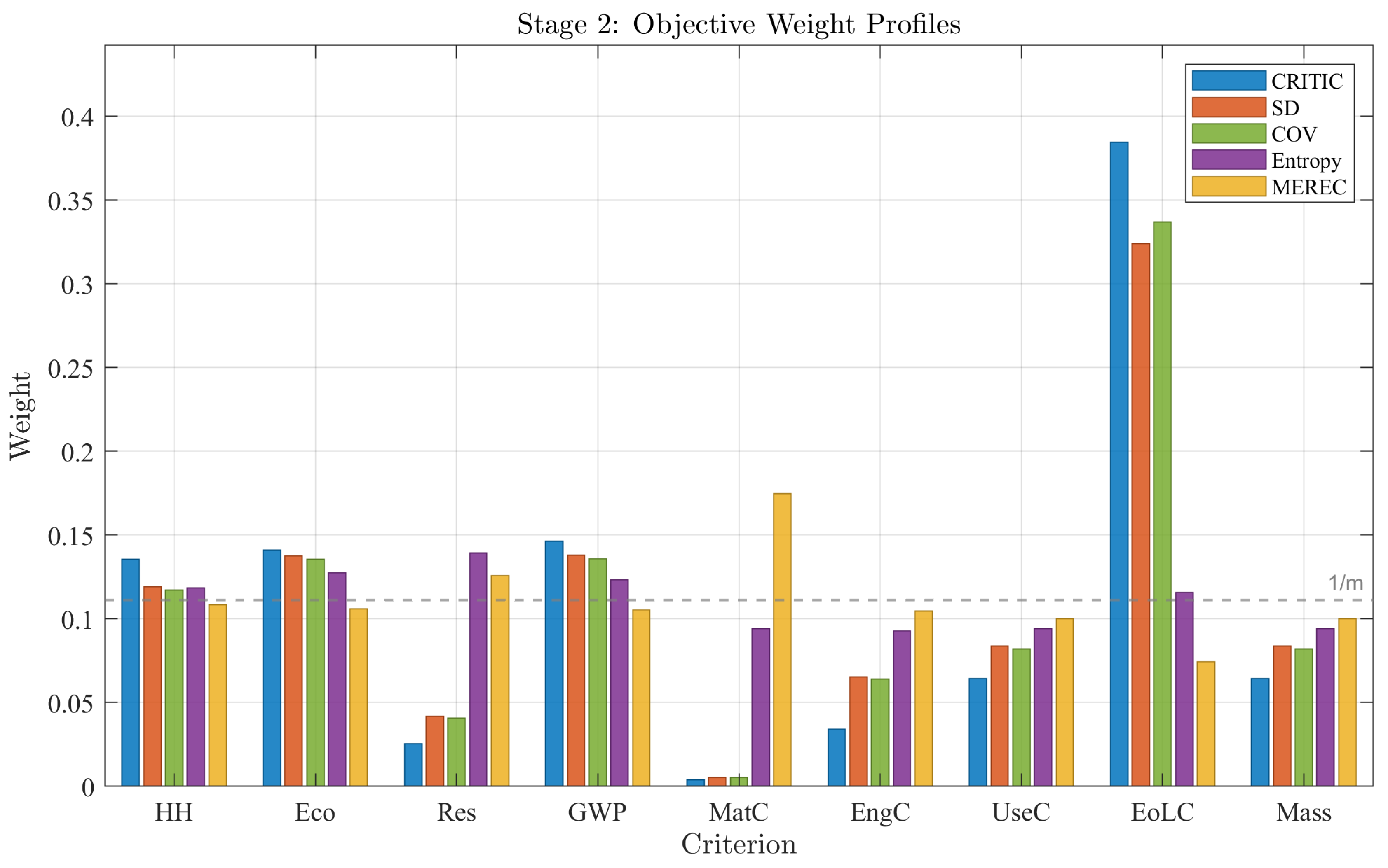
As Table 11 shows, the five methods do not produce the same weight profile. The dispersion-based methods, namely CRITIC, SD, and COV, concentrate their largest weight on criterion C8, the end-of-life cost. Their max/min ratios range from 59.9 to 92.6. This pattern is consistent with the much larger relative spread of end-of-life costs within the selected set, compared with the spread of material cost. In the present data, this is primarily associated with variations in overall mass and material distribution across the configurations. Material cost, by contrast, varies much less and therefore receives the lowest weight under these methods. The information-based methods, Entropy and MEREC, are much flatter, with max/min ratios of 1.5 and 2.3.
Figure 8.
Stage 2 objective weight profiles from five methods. The dashed line indicates equal weighting (). Dispersion-based methods (CRITIC, SD, COV) concentrate weight on C8 (EoL cost); information-based methods (Entropy, MEREC) distribute weight more uniformly.
Figure 8.
Stage 2 objective weight profiles from five methods. The dashed line indicates equal weighting (). Dispersion-based methods (CRITIC, SD, COV) concentrate weight on C8 (EoL cost); information-based methods (Entropy, MEREC) distribute weight more uniformly.
Even with these differences, the rankings obtained in Stage 2 agree very strongly at the top. The results are listed in Table 12.
All five methods place S01–S04 in ranks 1–4. This remains true even though the weighting rules are quite different. Within the reduced decision matrix used in Stage 2, Group G1 therefore keeps the leading positions under all five methods.
Below rank 4, the ordering is less consistent. CRITIC gives slightly better positions to Group G2, especially at ranks 5 and 6, whereas the other four methods place Group G4 ahead. This difference is linked mainly to criterion C8. Under CRITIC, end-of-life cost receives a particularly large weight, so the G4 alternatives, which use stainless steel in the outer tank, are penalised more strongly. When the weights are more evenly distributed, as in Entropy and MEREC, the environmental advantage of G4 is reflected more clearly and that group moves upward.
The corresponding TOPSIS proximity scores are shown in Figure 9.
5. Discussion
The two-stage analysis gives a rather stable picture of the LH2 tank alternatives. Group G1 (S01–S04, all-aluminium) remains in ranks 1–4 in all Stage 1 weighting scenarios and under all five objective weighting methods in Stage 2. This level of agreement is not typical in multi-criteria studies, although the claim should be understood only within the set of scenarios and weighting methods examined here.
One reason for this behaviour is the specific strength of Al2219-T8 (), which is more than twice that of AISI 316L. In the present design space, this gives lower tank mass among the metallic options. Lower mass means lower hydrogen demand during the use phase, and that effect is reflected in both environmental and cost-related criteria. In the current decision matrix, all evaluated criteria are influenced by mass, which drives the differences observed across the configurations. For the cases studied here, this creates a cumulative advantage for Group G1. This is not a formal proof of pairwise dominance over the full admissible weight region, but it helps explain why the leading group is not displaced under the weighting settings considered in this study.
A second issue is the relation among the criteria. The framework is organised by outcome categories, not by statistical independence. Each criterion has its own role in the LCA/LCC setting, but some are connected through common underlying factors. In particular, mass (C9) influences both the use-phase behaviour and the material- and process-related impacts across the system. The nine criteria should therefore not be interpreted as fully independent dimensions. This is not a modelling flaw; it follows from the physical fact that lighter tanks require less material and less hydrogen in operation. Even so, the effect of this dependence should be kept in mind. A useful follow-up would be to test whether the ranking remains the same under a reduced or decorrelated set of criteria, for example by removing C9 or one criterion that is strongly driven by mass.
The use of two different normalisation steps in Stage 2 also needs a brief explanation. It was not introduced for convenience. Vector normalisation was kept for weight computation because the objective weighting methods must still see the original variation across criteria. If Z-score standardisation were used at that stage, every criterion would have zero mean and unit variance, and the information needed by SD, COV, and CRITIC would be lost. Then the SD method would reduce to equal weights, and the COV method would be undefined. Vector normalisation, by contrast, keeps the column means positive and preserves the dispersion structure required by these methods. This also explains why the dispersion-based methods assign the largest weight to C8. In the reduced set, end-of-life cost varies much more than material cost, which is linked to the different end-of-life treatment of aluminium and steel.
The middle part of the ranking depends more strongly on the weighting assumptions. This is exactly where UW-TOPSIS is useful. Group G3 (S09–S12, Al/CFRP) moves from ranks 13–16 in the balanced case to ranks 5–9 when cost is favoured. This shift is mainly associated with the lower material cost of the CFRP-based option. Group G4 (S13–S16, Steel/Al) moves in the opposite direction. It stays competitive in the balanced and environmental cases, but drops when cost receives greater emphasis. Under a single fixed-weight ranking, this contrast between G3 and G4 would be much less visible. Here it is seen directly through the interval-based analysis.
The Stage 2 weight vectors may look uneven, especially for the dispersion-based methods. For CRITIC, the ratio between the largest and smallest weight reaches 92.6. That is large, but in the present data it reflects a property of the reduced set rather than a numerical artefact. End-of-life cost shows much stronger relative variation than some other criteria, and the weighting methods that respond to dispersion pick up exactly that feature. Entropy and MEREC are flatter by construction, yet they still produce the same top four alternatives. Under the current modelling assumptions, this agreement supports the stability of the leading group.
The analysis also has clear limits. The results depend on the life cycle inventory, the chosen system boundaries, and the modelling assumptions used throughout the study. This is especially true for the use-phase model, where hydrogen demand is linked to mass through the Piaggio P. 180 reference aircraft. A different aircraft, mission profile, or hydrogen supply pathway could change the strength of the mass-related advantage observed here. The technical side of the problem is represented only by mass. Other important properties, such as hydrogen permeability, cryogenic durability, inspectability, damage tolerance, and thermal performance, are discussed in the introduction but are not included as explicit criteria. The comparison is also limited to metallic and CFRP solutions; other candidate materials, such as thermoplastic composites or aluminium–lithium alloys, are outside the scope of the present work. In addition, no formal propagation of uncertainty from the LCA/LCC inputs to the decision matrix has been carried out, no sensitivity study has been performed for alternative Stage 1 normalisation choices, and the social dimension of sustainability has not been included.
6. Conclusions
This study proposed a two-stage multi-criteria framework for the sustainability assessment of liquid hydrogen aircraft tank configurations. In the first stage, UW-TOPSIS was used to examine the design space under interval-valued weights, without assuming fixed preferences in advance. In the second stage, the reduced set of alternatives was re-evaluated with a standardised TOPSIS variant (vector-normalised weights, Z-standardised distances) and five objective weighting methods.
A clear result was observed in all analyses carried out here. The all-aluminium configurations S01–S04 (Group G1) remained in ranks 1–4 in all four weighting scenarios and under all five objective weighting methods. Thus, the same top four alternatives were obtained in nine separate evaluations. The middle part of the ranking was less stable. Mixed-material configurations changed position by as many as 8 ranks across the scenarios, which shows that their evaluation depends much more strongly on the adopted design priorities. From the methodological side, the use of vector normalisation for weight computation and Z-score normalisation for distance computation was necessary. A single normalisation scheme would have produced known problems, including degenerate SD weights and an undefined COV method.
The framework is intended for cases in which criterion weights cannot yet be justified at the start of the analysis. The final ranking is then obtained only after the reduced set has been identified and the weights have been derived from its decision matrix. Future work may extend the comparison to additional structural materials, include further technical criteria such as thermal performance, and incorporate the social dimension of sustainability.
Author Contributions
Conceptualization, A.A., D.G.S. and K.T.; methodology, A.A., D.G.S., K.T., G.T. and G.L.; software, A.A. and D.G.S.; validation, A.A., D.G.S., K.T., G.T. and G.L.; formal analysis, A.A., D.G.S. and K.T.; investigation, A.A., D.G.S., K.T., G.T. and G.L.; resources, K.T. and G.L.; data curation, A.A., D.G.S., K.T., G.T. and G.L.; writing—original draft preparation, A.A. and D.G.S.; writing—review and editing, A.A., D.G.S., K.T., G.T. and G.L.; supervision, K.T. and G.L.; project administration, K.T. and G.L.; funding acquisition, K.T. and G.L. All authors have read and agreed to the published version of the manuscript.
Funding
This research was partially funded by the Horizon Europe Clean Aviation Project H2ELIOS, grant number 101102003.
Data Availability Statement
All data supporting the findings of this study are contained within the article and its appendices.
Conflicts of Interest
The authors declare no conflicts of interest.
Abbreviations
The following abbreviations are used in this manuscript:
| LH2 | Liquid hydrogen |
| LCA | Life Cycle Assessment |
| LCC | Life Cycle Costing |
| LCI | Life Cycle Inventory |
| MCDM | Multi-Criteria Decision Making |
| TOPSIS | Technique for Order Preference by Similarity to Ideal Solution |
| UW-TOPSIS | Unweighted TOPSIS |
| CRITIC | Criteria Importance Through Intercriteria Correlation |
| SD | Standard Deviation |
| COV | Coefficient of Variation |
| MEREC | Method based on the Removal Effects of Criteria |
| CFRP | Carbon Fibre Reinforced Polymer |
| GFRP | Glass Fibre Reinforced Polymer |
| PTFE | Polytetrafluoroethylene |
| GWP | Global Warming Potential |
| SAF | Sustainable Aviation Fuel |
| PIS | Positive Ideal Solution |
| NIS | Negative Ideal Solution |
| SQP | Sequential Quadratic Programming |
Appendix A. Material Alternatives for Tank Components
The material combinations for the four variable structural components are summarised in Table A1–Table A4. Each table lists the candidate materials at the subcomponent level. Common materials (e.g. PTFE liners, BaSO4 seals, GFRP spacers) appear in every alternative and are therefore not treated as design variables; they are, however, included in all environmental, economic, and technical calculations.

Table A1.
Inner tank alternatives.
| Inner tank A | Inner tank B | Inner tank C |
|---|---|---|
| AISI 316L stainless steel | Al2219-T8 | PC + 20 wt% CF |
| PTFE (Polytetrafluoroethylene) | PTFE (Polytetrafluoroethylene) | PTFE (Polytetrafluoroethylene) |
| BaSO4 | BaSO4 | BaSO4 |
Table A2.
Inner tank support alternatives.
| Inner tank supports A | Inner tank supports B |
|---|---|
| Spring steel 17-4PH | Spring steel 17-4PH |
| AISI 316L stainless steel | Al2219-T8 |
| GFRP | GFRP |
Table A3.
Outer tank support alternatives.
| Outer tank supports A | Outer tank supports B |
|---|---|
| AISI 316L stainless steel | Al2219-T8 |
Table A4.
Outer tank alternatives.
| Outer tank A | Outer tank B |
|---|---|
| UD tape CFRP | UD tape CFRP |
| Fabric CFRP | Fabric CFRP |
| PTFE (Polytetrafluoroethylene) | PTFE (Polytetrafluoroethylene) |
| BaSO4 | BaSO4 |
| AISI 316L stainless steel (auxiliary) | Al2219-T8 (auxiliary) |
| AISI 316L stainless steel (welded elements) | Al2219-T8 (welded elements) |
| AISI 316L stainless steel (systems assembly) | Al2219-T8 (systems assembly) |
Appendix B. Mass Distribution
Table A5 presents the mass distribution per component for the reference scenario (Scenario 1), in which Al2219-T8 is the baseline material for all main structural components.
Table A5.
Mass distribution per component for the reference scenario (Scenario 1).
| Component | Material | Mass (kg) |
|---|---|---|
| Outer tank | Al2219-T8 | 177.51 |
| UD tape CFRP | 65.00 | |
| Fabric CFRP | 10.60 | |
| PTFE BaSO4 | 1.599 | |
| Inner tank | Al2219-T8 | 148.04 |
| PTFE BaSO4 | 0.84 | |
| Outer tank supports | Al2219-T8 | 10.71 |
| Al2219-T8 | 4.196 | |
| Inner tank supports | Spring steel 17-4PH | 14.867 |
| GFRP | 0.237 | |
| External insulation | Closed cell insulation material | 268.26 |
| Internal insulation | Open cell insulation material | 180.21 |
Appendix C. UW-TOPSIS Proximity Intervals for Cases 2–4
Table A6–Table A8 present the complete UW-TOPSIS proximity intervals under the environmental, cost, and technical scenarios, respectively. These tables complement the balanced-scenario results in Table 8 and underpin the cross-case comparison of Table 9.
Table A6.
UW-TOPSIS proximity intervals under the environmental scenario (Case 2).
| Rank | Alt. | Group | Score | Width | ||
|---|---|---|---|---|---|---|
| 1 | S01 | G1 | 0.8337 | 0.8860 | 1.7197 | 0.0522 |
| 2 | S02 | G1 | 0.8262 | 0.8803 | 1.7064 | 0.0541 |
| 3 | S03 | G1 | 0.8143 | 0.8710 | 1.6853 | 0.0567 |
| 4 | S04 | G1 | 0.8066 | 0.8650 | 1.6716 | 0.0583 |
| 5 | S13 | G4 | 0.4850 | 0.7321 | 1.2170 | 0.2471 |
| 6 | S14 | G4 | 0.4794 | 0.7282 | 1.2076 | 0.2488 |
| 7 | S05 | G2 | 0.5518 | 0.6495 | 1.2013 | 0.0977 |
| 8 | S15 | G4 | 0.4706 | 0.7220 | 1.1926 | 0.2514 |
| 9 | S06 | G2 | 0.5435 | 0.6424 | 1.1859 | 0.0988 |
| 10 | S16 | G4 | 0.4650 | 0.7179 | 1.1829 | 0.2529 |
| 11 | S07 | G2 | 0.5311 | 0.6316 | 1.1627 | 0.1006 |
| 12 | S08 | G2 | 0.5231 | 0.6248 | 1.1479 | 0.1017 |
| 13 | S09 | G3 | 0.3453 | 0.6292 | 0.9744 | 0.2839 |
| 14 | S10 | G3 | 0.3415 | 0.6253 | 0.9668 | 0.2838 |
| 15 | S11 | G3 | 0.3358 | 0.6191 | 0.9549 | 0.2833 |
| 16 | S12 | G3 | 0.3322 | 0.6151 | 0.9473 | 0.2829 |
| 17 | S17 | G5 | 0.2990 | 0.5544 | 0.8534 | 0.2554 |
| 18 | S18 | G5 | 0.2947 | 0.5488 | 0.8435 | 0.2541 |
| 19 | S19 | G5 | 0.2882 | 0.5400 | 0.8282 | 0.2518 |
| 20 | S20 | G5 | 0.2842 | 0.5344 | 0.8186 | 0.2502 |
| 21 | S21 | G6 | 0.2317 | 0.3619 | 0.5936 | 0.1302 |
| 22 | S22 | G6 | 0.2250 | 0.3550 | 0.5800 | 0.1299 |
| 23 | S23 | G6 | 0.2152 | 0.3444 | 0.5596 | 0.1292 |
| 24 | S24 | G6 | 0.2090 | 0.3377 | 0.5467 | 0.1287 |
Table A7.
UW-TOPSIS proximity intervals under the cost scenario (Case 3).
| Rank | Alt. | Group | Score | Width | ||
|---|---|---|---|---|---|---|
| 1 | S01 | G1 | 0.8440 | 0.8877 | 1.7317 | 0.0438 |
| 2 | S02 | G1 | 0.8367 | 0.8820 | 1.7187 | 0.0454 |
| 3 | S03 | G1 | 0.8253 | 0.8727 | 1.6980 | 0.0474 |
| 4 | S04 | G1 | 0.8180 | 0.8665 | 1.6845 | 0.0485 |
| 5 | S09 | G3 | 0.4543 | 0.7708 | 1.2252 | 0.3165 |
| 6 | S10 | G3 | 0.4502 | 0.7679 | 1.2181 | 0.3177 |
| 7 | S11 | G3 | 0.4438 | 0.7630 | 1.2068 | 0.3192 |
| 8 | S05 | G2 | 0.5700 | 0.6358 | 1.2058 | 0.0658 |
| 9 | S12 | G3 | 0.4397 | 0.7597 | 1.1994 | 0.3200 |
| 10 | S06 | G2 | 0.5615 | 0.6282 | 1.1896 | 0.0667 |
| 11 | S07 | G2 | 0.5485 | 0.6165 | 1.1650 | 0.0679 |
| 12 | S08 | G2 | 0.5402 | 0.6090 | 1.1492 | 0.0687 |
| 13 | S13 | G4 | 0.3700 | 0.6382 | 1.0082 | 0.2682 |
| 14 | S14 | G4 | 0.3637 | 0.6335 | 0.9972 | 0.2697 |
| 15 | S15 | G4 | 0.3539 | 0.6260 | 0.9799 | 0.2720 |
| 16 | S16 | G4 | 0.3477 | 0.6211 | 0.9688 | 0.2734 |
| 17 | S21 | G6 | 0.2611 | 0.4136 | 0.6747 | 0.1526 |
| 18 | S22 | G6 | 0.2552 | 0.4065 | 0.6617 | 0.1513 |
| 19 | S23 | G6 | 0.2464 | 0.3955 | 0.6419 | 0.1491 |
| 20 | S17 | G5 | 0.1789 | 0.4532 | 0.6321 | 0.2744 |
| 21 | S24 | G6 | 0.2409 | 0.3884 | 0.6294 | 0.1475 |
| 22 | S18 | G5 | 0.1755 | 0.4482 | 0.6237 | 0.2726 |
| 23 | S19 | G5 | 0.1706 | 0.4402 | 0.6108 | 0.2695 |
| 24 | S20 | G5 | 0.1678 | 0.4351 | 0.6029 | 0.2673 |
Table A8.
UW-TOPSIS proximity intervals under the technical scenario (Case 4).
| Rank | Alt. | Group | Score | Width | ||
|---|---|---|---|---|---|---|
| 1 | S01 | G1 | 0.8475 | 0.8994 | 1.7469 | 0.0519 |
| 2 | S02 | G1 | 0.8403 | 0.8942 | 1.7345 | 0.0538 |
| 3 | S03 | G1 | 0.8291 | 0.8855 | 1.7145 | 0.0564 |
| 4 | S04 | G1 | 0.8218 | 0.8796 | 1.7014 | 0.0578 |
| 5 | S05 | G2 | 0.5791 | 0.6523 | 1.2314 | 0.0732 |
| 6 | S06 | G2 | 0.5709 | 0.6447 | 1.2156 | 0.0738 |
| 7 | S07 | G2 | 0.5585 | 0.6330 | 1.1915 | 0.0745 |
| 8 | S08 | G2 | 0.5506 | 0.6256 | 1.1762 | 0.0749 |
| 9 | S13 | G4 | 0.4582 | 0.6914 | 1.1496 | 0.2332 |
| 10 | S14 | G4 | 0.4522 | 0.6870 | 1.1392 | 0.2348 |
| 11 | S15 | G4 | 0.4429 | 0.6801 | 1.1229 | 0.2372 |
| 12 | S16 | G4 | 0.4369 | 0.6755 | 1.1124 | 0.2387 |
| 13 | S09 | G3 | 0.3921 | 0.6599 | 1.0519 | 0.2678 |
| 14 | S10 | G3 | 0.3880 | 0.6559 | 1.0439 | 0.2678 |
| 15 | S11 | G3 | 0.3818 | 0.6495 | 1.0313 | 0.2677 |
| 16 | S12 | G3 | 0.3779 | 0.6453 | 1.0232 | 0.2674 |
| 17 | S17 | G5 | 0.2642 | 0.5069 | 0.7711 | 0.2427 |
| 18 | S18 | G5 | 0.2599 | 0.5014 | 0.7614 | 0.2415 |
| 19 | S19 | G5 | 0.2535 | 0.4928 | 0.7463 | 0.2393 |
| 20 | S20 | G5 | 0.2496 | 0.4874 | 0.7369 | 0.2378 |
| 21 | S21 | G6 | 0.2224 | 0.3673 | 0.5896 | 0.1449 |
| 22 | S22 | G6 | 0.2169 | 0.3603 | 0.5771 | 0.1434 |
| 23 | S23 | G6 | 0.2087 | 0.3495 | 0.5583 | 0.1408 |
| 24 | S24 | G6 | 0.2037 | 0.3427 | 0.5464 | 0.1390 |
References
- European Commission. 2050 Long-Term Strategy . Available online: https://climate.ec.europa.eu/eu-action/climate-strategies-targets/2050-long-term-strategy_en.
- Gallagher, C.; Stuart, C.; Spence, S. Liquid Hydrogen and Synthetic Sustainable Aviation Fuel: A European Airline Case Study. Proceedings of GPPS Chania24, September 2024. [Google Scholar] [CrossRef]
- Vogiantzi, C.; Tserpes, K. On the Definition, Assessment, and Enhancement of Circular Economy across Various Industrial Sectors: A Literature Review and Recent Findings. Sustainability 2023, 15(23), 16532. [Google Scholar] [CrossRef]
- Whittle, J.W.; Callander, K.; Akure, M.; Kachwala, F.; Koh, S.C.L. A New High-Level Life Cycle Assessment Framework for Evaluating Environmental Performance: An Aviation Case Study. J. Clean. Prod. 2024, 471, 143440. [Google Scholar] [CrossRef]
- Kurzawska-Pietrowicz, P. Life Cycle Emission of Selected Sustainable Aviation Fuels—A Review. Transp. Res. Procedia 2023, 75, 77–85. [Google Scholar] [CrossRef]
- Pinto, D.B.S.B. Hydrogen Aircraft Conceptual Design and Life Cycle Assessment . Master’s Thesis, Instituto Superior Técnico, Universidade de Lisboa, Portugal, July 2022. [Google Scholar]
- Boddorff, A.K. Choosing the Right Stuff: Material Selection for Liquid Hydrogen Aircraft Cryotanks; NASA Technical Memorandum NASA/TM-20250007133; National Aeronautics and Space Administration, Langley Research Center: Hampton, VA, USA, 2025; Available online: https://ntrs.nasa.gov/citations/20250007133.
- Revolutionizing Aircraft Materials and Processes; Pantelakis, S., Tserpes, K., Eds.; Springer International Publishing: Cham, 2020. [Google Scholar] [CrossRef]
- Benitez, A.; et al. Ecological Assessment of Fuel Cell Electric Vehicles with Special Focus on Type IV Carbon Fiber Hydrogen Tank. J. Clean. Prod. 2021, 278, 123277. [Google Scholar] [CrossRef]
- Ye, L.; Lu, L. Environmental and Economic Evaluation of the High-Pressured and Cryogenic Vessels for Hydrogen Storage on the Sedan. Int. J. Low.-Carbon Technol. 2023, 18, 144–149. [Google Scholar] [CrossRef]
- Energy Systems Evaluation . In Green Energy and Technology; Ren, J., Ed.; Springer: Cham, 2021; Volume 2. [Google Scholar] [CrossRef]
- Anagnostopoulou, A.; Sotiropoulos, D.; Tserpes, K. A Robust Sustainability Assessment Methodology for Aircraft Parts: Application to a Fuselage Panel. Sustainability 2025, 17(8), 3299. [Google Scholar] [CrossRef]
- Anagnostopoulou, A.; Sotiropoulos, D.; Sioutis, I.; Tserpes, K. Sustainability-Driven Design Optimization of Aircraft Parts Using Mathematical Modelling. Aerospace 2026, 13(1), 95. [Google Scholar] [CrossRef]
- Liern, V.; Pérez-Gladish, B. Multiple Criteria Ranking Method Based on Functional Proximity Index: Un-weighted TOPSIS. Ann. Oper. Res. 2022, 311(2), 1109–1137. [Google Scholar] [CrossRef]
- Liern, V.; Pérez-Gladish, B. Building Composite Indicators With Unweighted-TOPSIS. IEEE Trans. Eng. Manag. 2023, 70(5), 1871–1880. [Google Scholar] [CrossRef]
- ISO 14040:2006; Environmental Management—Life Cycle Assessment—Principles and Framework. ISO: Geneva, Switzerland, 2006.
- ISO 14044:2006; Environmental Management—Life Cycle Assessment—Requirements and Guidelines. ISO: Geneva, Switzerland, 2006.
- Cañós, L.; Liern, V. Soft Computing-Based Aggregation Methods for Human Resource Management. Eur. J. Oper. Res. 2008, 189(2), 669–681. [Google Scholar] [CrossRef]
- Hwang, C.-L.; Yoon, K. Multiple Attribute Decision Making . In Lecture Notes in Economics and Mathematical Systems; Springer: Berlin, 1981; Vol. 186. [Google Scholar]
- Diakoulaki, D.; Mavrotas, G.; Papayannakis, L. Determining Objective Weights in Multiple Criteria Problems: The CRITIC Method. Comput. Oper. Res. 1995, 22(7), 763–770. [Google Scholar] [CrossRef]
- Zelený, M. Multiple Criteria Decision Making; McGraw-Hill: New York, 1982. [Google Scholar]
- Wang, Y.-M.; Luo, Y. Integration of Correlations with Standard Deviations for Determining Attribute Weights in Multiple Attribute Decision Making. Math. Comput. Model. 2010, 51(1–2), 1–12. [Google Scholar] [CrossRef]
- Keshavarz-Ghorabaee, M.; Amiri, M.; Zavadskas, E.K.; Turskis, Z.; Antucheviciene, J. Determination of Objective Weights Using a New Method Based on the Removal Effects of Criteria (MEREC). Symmetry 2021, 13(4), 525. [Google Scholar] [CrossRef]
- Keshavarz-Ghorabaee, M. Assessment of Distribution Center Locations Using a Multi-Expert Subjective–Objective Decision-Making Approach. Sci. Rep. 2021, 11, 19461. [Google Scholar] [CrossRef] [PubMed]
| 1 | Z-score standardisation is invariant under positive column-wise rescaling: if with , then . It therefore produces the same whether it is applied to or to the vector-normalised matrix . The use of both and reflects their different roles in the method: weight computation and distance computation, respectively. |
Figure 2.
Two-stage sustainability assessment framework for LH2 tank configurations. Stage 1 uses UW-TOPSIS for design-space exploration and screening, whereas Stage 2 applies a standardised TOPSIS variant (vector-normalised weights, Z-standardised distances) with objective weighting methods to obtain the final sustainability ranking.
Figure 2.
Two-stage sustainability assessment framework for LH2 tank configurations. Stage 1 uses UW-TOPSIS for design-space exploration and screening, whereas Stage 2 applies a standardised TOPSIS variant (vector-normalised weights, Z-standardised distances) with objective weighting methods to obtain the final sustainability ranking.
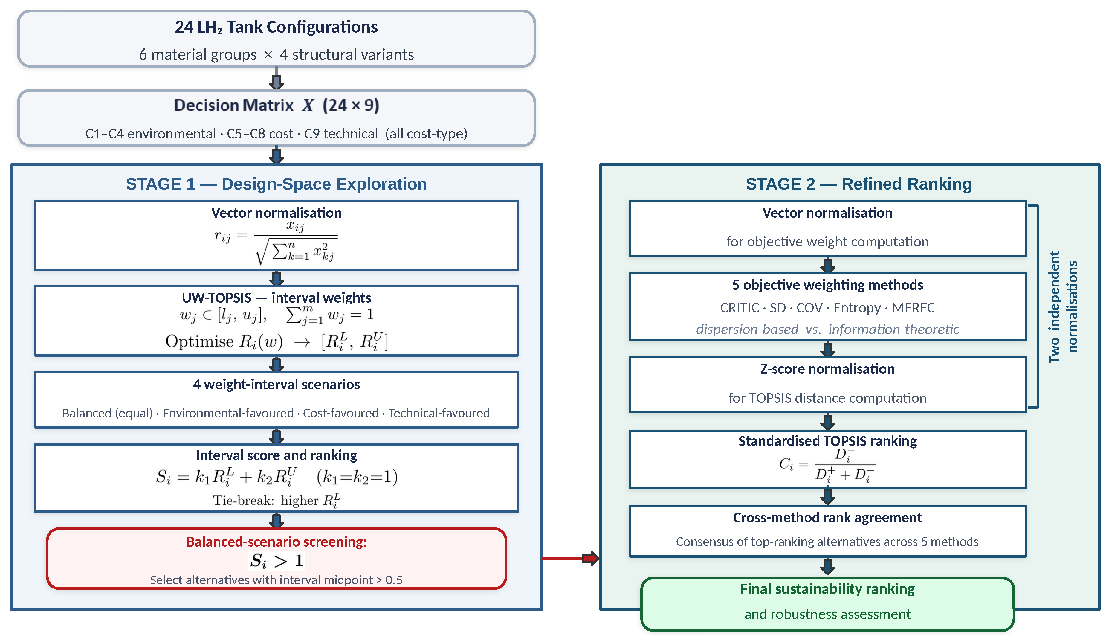
Figure 3.
UW-TOPSIS proximity intervals for the LH2 tank design alternatives in the balanced scenario (Case 1). The alternatives are arranged by material group (G1–G6) and, within each group, by rank. Each horizontal bar shows the interval .
Figure 3.
UW-TOPSIS proximity intervals for the LH2 tank design alternatives in the balanced scenario (Case 1). The alternatives are arranged by material group (G1–G6) and, within each group, by rank. Each horizontal bar shows the interval .
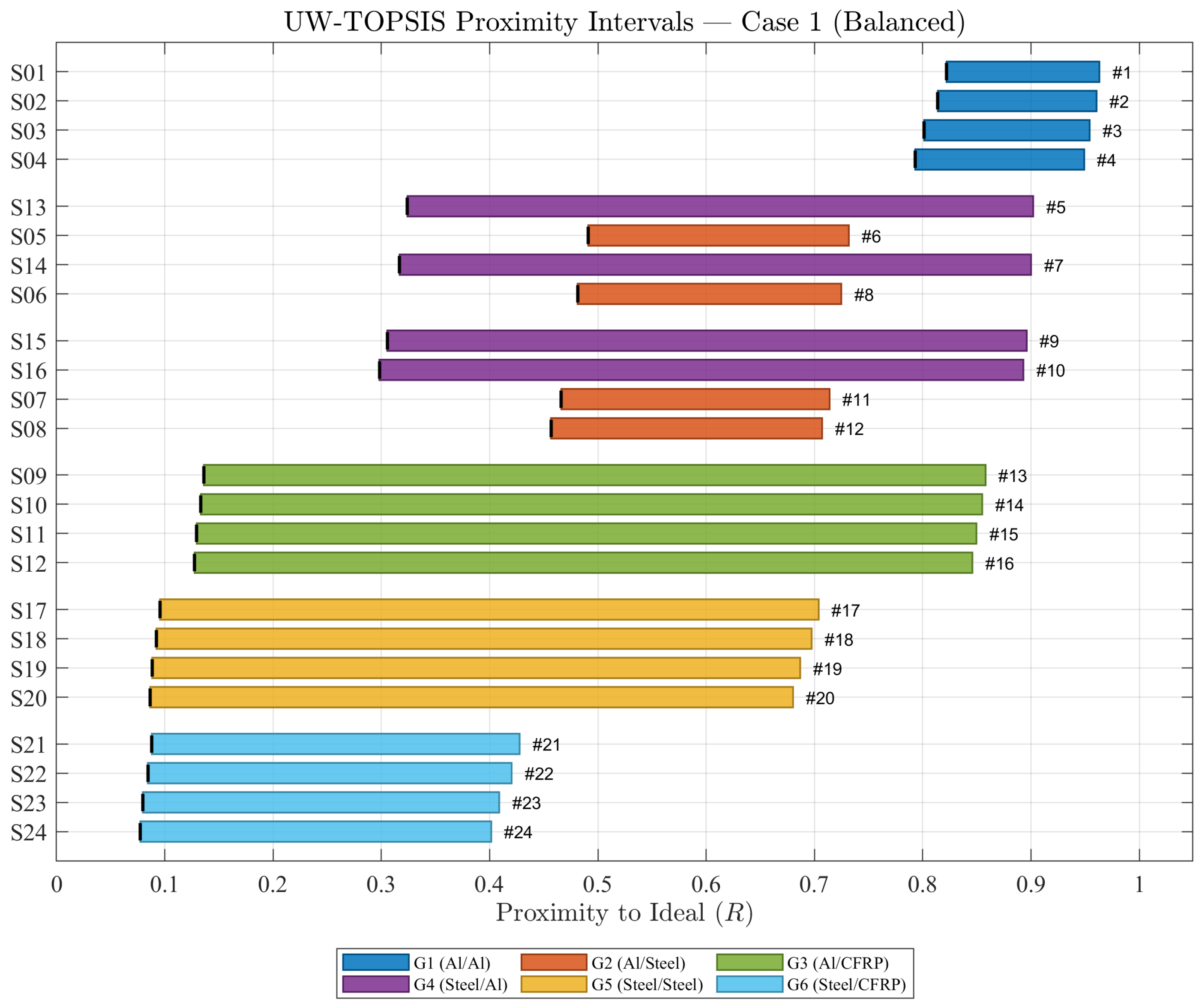
Figure 4.
Heatmap of LH2 tank alternative rankings across four weighting scenarios. Darker shading indicates better (lower) rank. Alternatives are ordered by their balanced-scenario rank.
Figure 4.
Heatmap of LH2 tank alternative rankings across four weighting scenarios. Darker shading indicates better (lower) rank. Alternatives are ordered by their balanced-scenario rank.
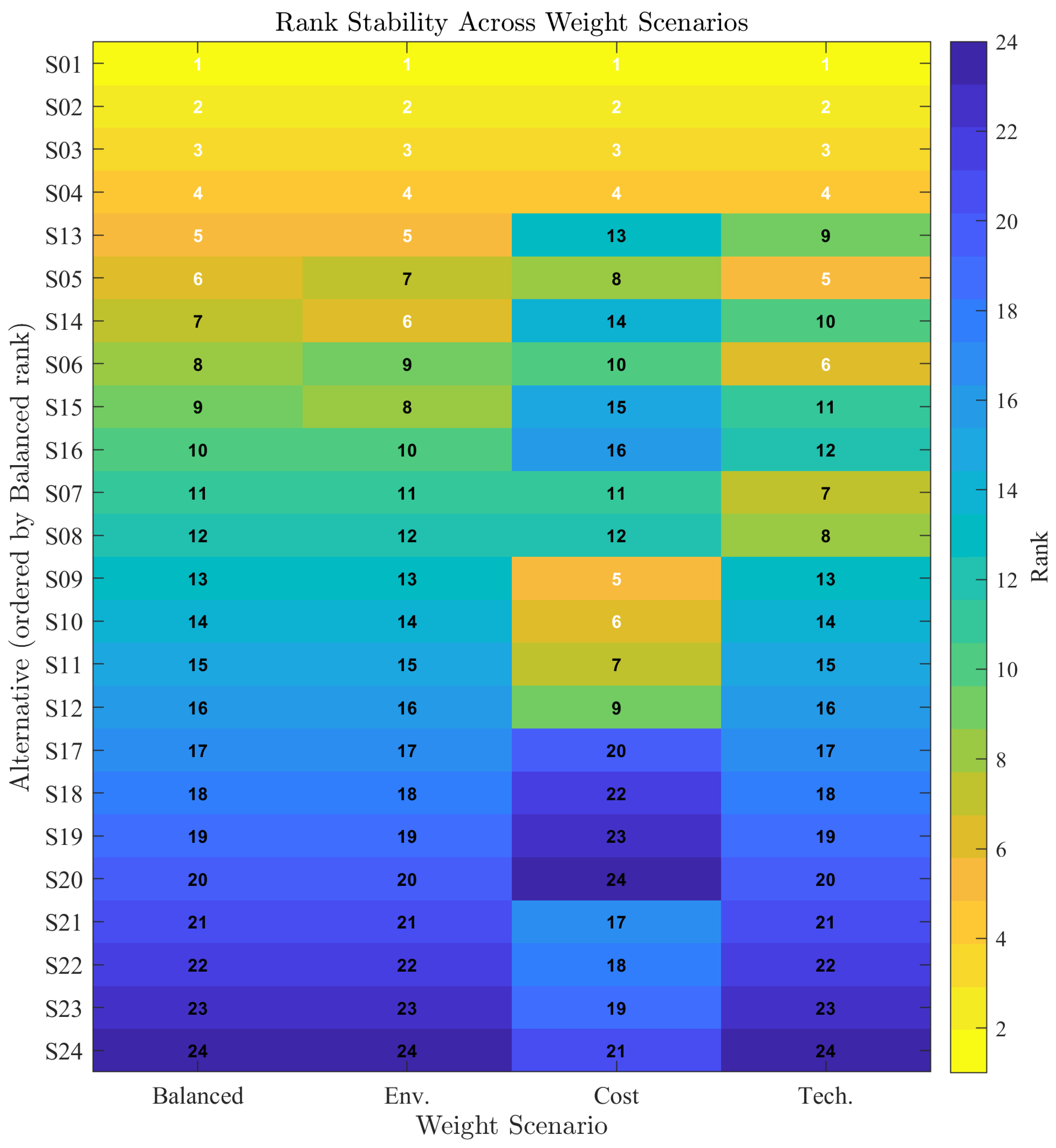
Figure 5.
UW-TOPSIS proximity intervals under the environmental scenario (Case 2).
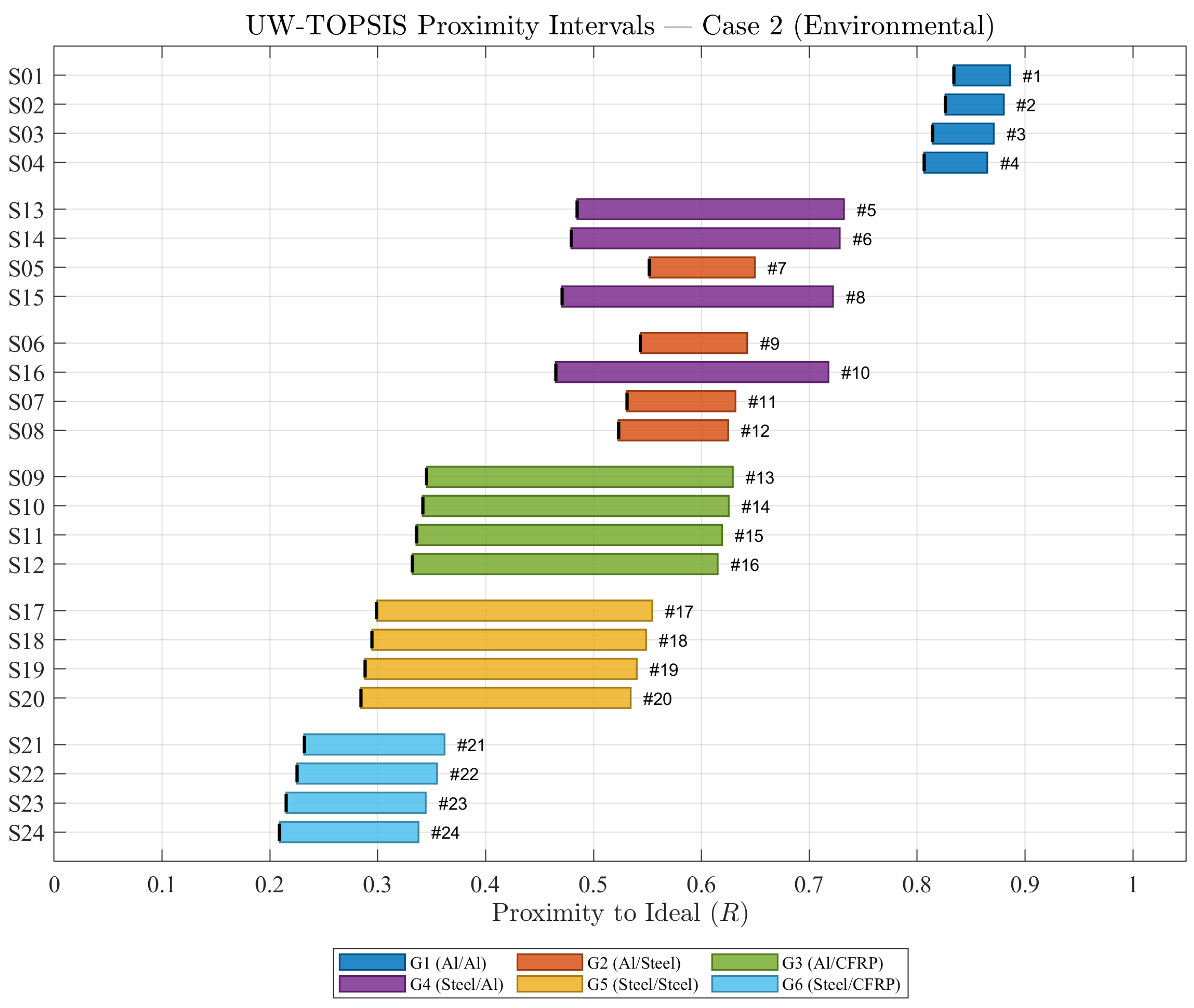
Figure 6.
UW-TOPSIS proximity intervals under the cost scenario (Case 3).
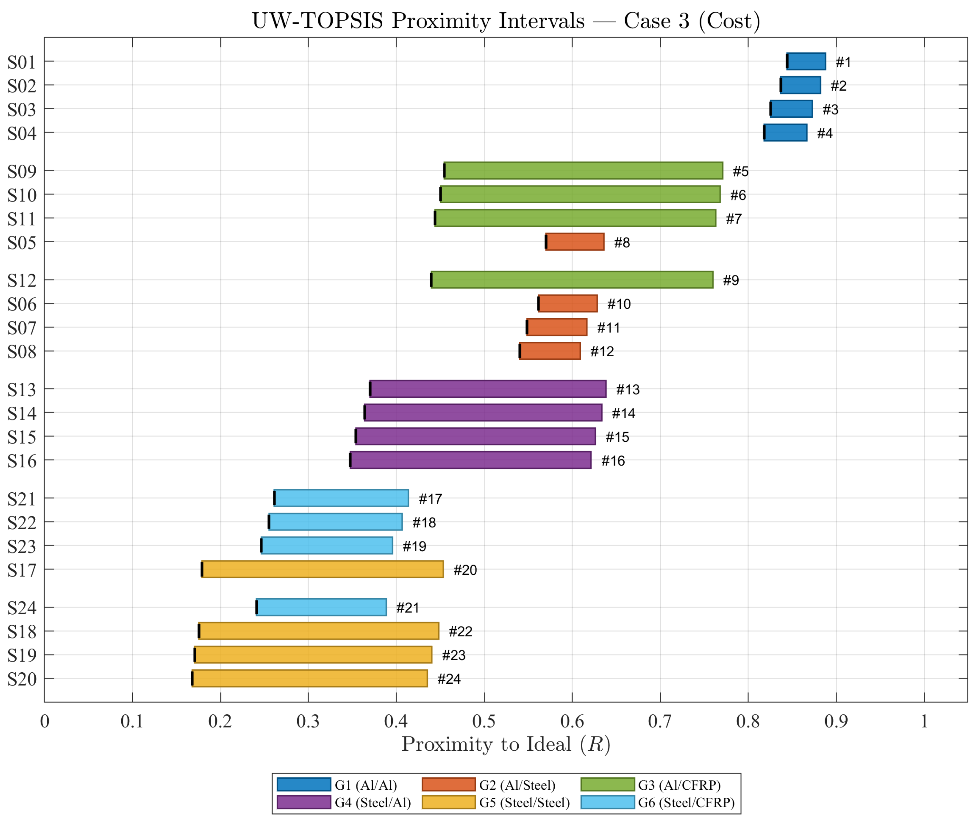
Figure 7.
UW-TOPSIS proximity intervals under the technical scenario (Case 4).
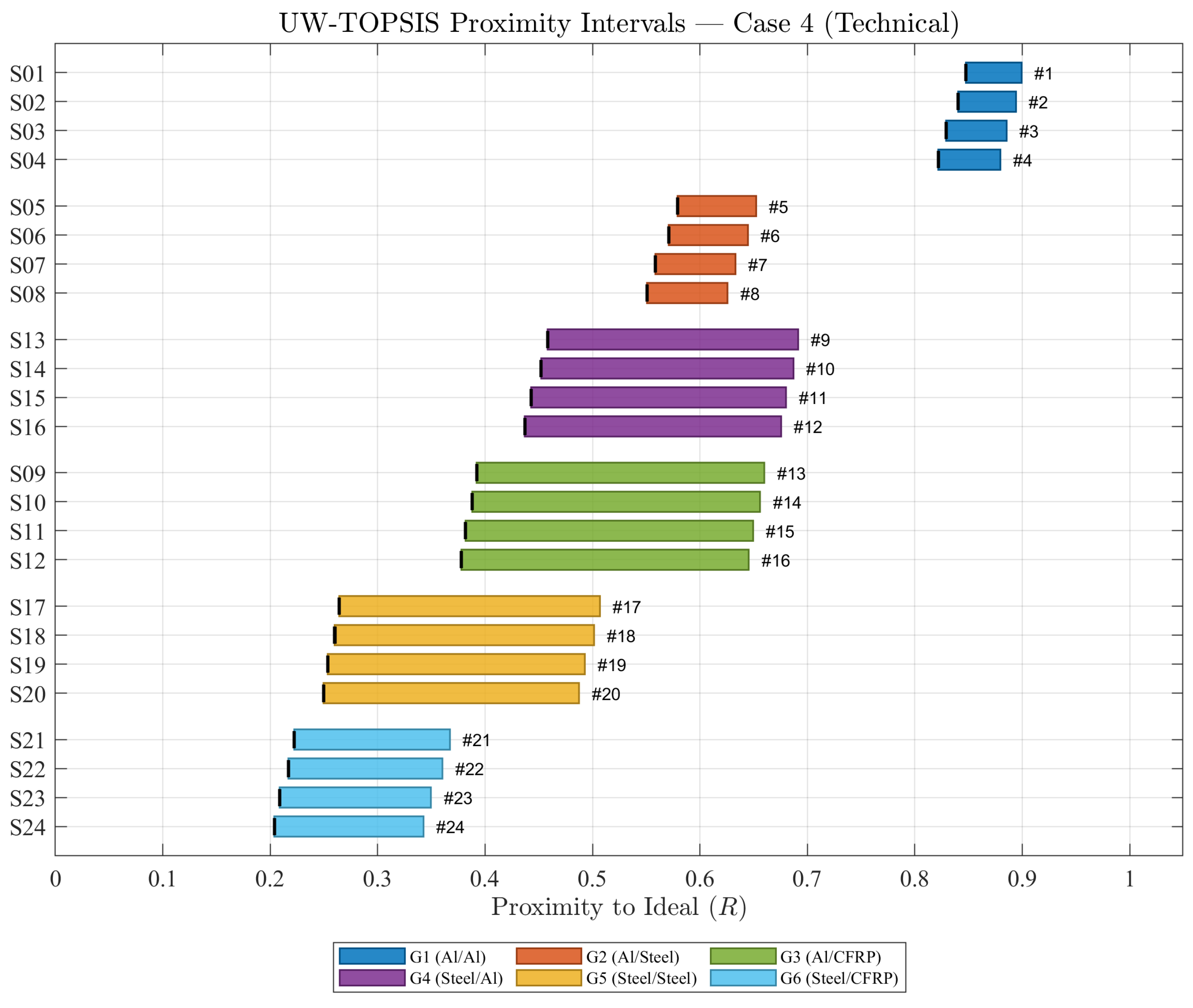
Figure 9.
Stage 2 standardised TOPSIS proximity scores on the reduced top-12 set under five objective weighting methods.
Figure 9.
Stage 2 standardised TOPSIS proximity scores on the reduced top-12 set under five objective weighting methods.
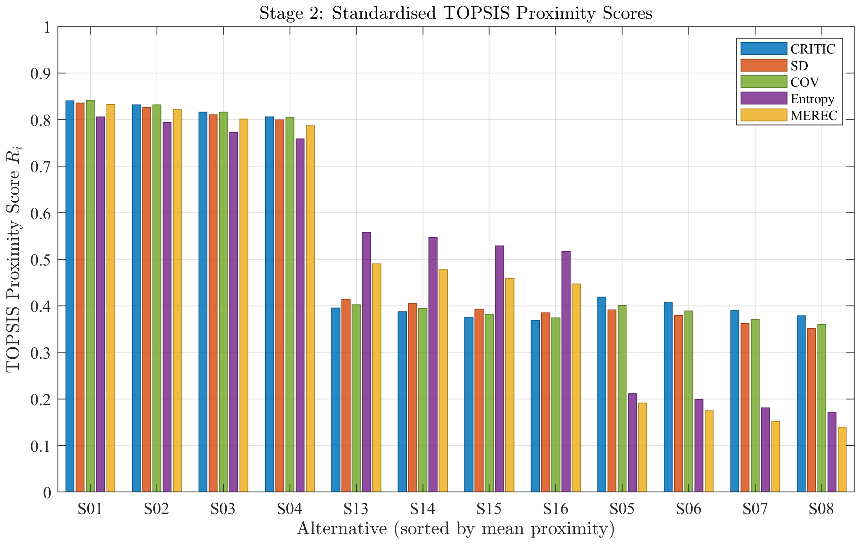
Table 1.
Characteristics of the LH2 storage tank design alternatives.
| ID | Outer tank | Inner tank | Outer supports | Inner supports |
|---|---|---|---|---|
| S01 | Al2219-T8 | Al2219-T8 | Al2219-T8 | Al2219-T8 |
| S02 | Al2219-T8 | Al2219-T8 | Al2219-T8 | AISI 316L |
| S03 | Al2219-T8 | Al2219-T8 | AISI 316L | Al2219-T8 |
| S04 | Al2219-T8 | Al2219-T8 | AISI 316L | AISI 316L |
| S05 | Al2219-T8 | AISI 316L | Al2219-T8 | Al2219-T8 |
| S06 | Al2219-T8 | AISI 316L | Al2219-T8 | AISI 316L |
| S07 | Al2219-T8 | AISI 316L | AISI 316L | Al2219-T8 |
| S08 | Al2219-T8 | AISI 316L | AISI 316L | AISI 316L |
| S09 | Al2219-T8 | CFRP | Al2219-T8 | Al2219-T8 |
| S10 | Al2219-T8 | CFRP | Al2219-T8 | AISI 316L |
| S11 | Al2219-T8 | CFRP | AISI 316L | Al2219-T8 |
| S12 | Al2219-T8 | CFRP | AISI 316L | AISI 316L |
| S13 | AISI 316L | Al2219-T8 | Al2219-T8 | Al2219-T8 |
| S14 | AISI 316L | Al2219-T8 | Al2219-T8 | AISI 316L |
| S15 | AISI 316L | Al2219-T8 | AISI 316L | Al2219-T8 |
| S16 | AISI 316L | Al2219-T8 | AISI 316L | AISI 316L |
| S17 | AISI 316L | AISI 316L | Al2219-T8 | Al2219-T8 |
| S18 | AISI 316L | AISI 316L | Al2219-T8 | AISI 316L |
| S19 | AISI 316L | AISI 316L | AISI 316L | Al2219-T8 |
| S20 | AISI 316L | AISI 316L | AISI 316L | AISI 316L |
| S21 | AISI 316L | CFRP | Al2219-T8 | Al2219-T8 |
| S22 | AISI 316L | CFRP | Al2219-T8 | AISI 316L |
| S23 | AISI 316L | CFRP | AISI 316L | Al2219-T8 |
| S24 | AISI 316L | CFRP | AISI 316L | AISI 316L |
Table 2.
Material group classification of the LH2 tank design alternatives.
| Group | Outer tank | Inner tank | Alternatives |
|---|---|---|---|
| G1 | Al2219-T8 | Al2219-T8 | S01–S04 |
| G2 | Al2219-T8 | AISI 316L | S05–S08 |
| G3 | Al2219-T8 | CFRP | S09–S12 |
| G4 | AISI 316L | Al2219-T8 | S13–S16 |
| G5 | AISI 316L | AISI 316L | S17–S20 |
| G6 | AISI 316L | CFRP | S21–S24 |
Table 3.
Criteria description and categorisation for the sustainability assessment of LH2 tank configurations.
Table 3.
Criteria description and categorisation for the sustainability assessment of LH2 tank configurations.
| Criterion | Description | Category | Impact type |
|---|---|---|---|
| C1 | Human health (DALYs) | Environment | Minimise |
| C2 | Ecosystems (species·yr) | Environment | Minimise |
| C3 | Resources (USD 2013) | Environment | Minimise |
| C4 | Global warming potential (kg CO2 eq.) | Environment | Minimise |
| C5 | Material cost (EUR) | Cost | Minimise |
| C6 | Energy cost (EUR) | Cost | Minimise |
| C7 | Use cost (EUR) | Cost | Minimise |
| C8 | End-of-life cost (EUR) | Cost | Minimise |
| C9 | Mass (kg) | Technical | Minimise |
Table 4.
Mechanical properties and specific strength of alternative materials.
| Material | Tensile strength (MPa) | Density () | Specific strength (/g) |
|---|---|---|---|
| AISI 316L | 580 | 7.97 | 72.77 |
| Al2219-T8 | 450 | 2.84 | 158.45 |
| PC + 20% CF | 57.92 | 1.30 | 44.55 |
Table 5.
Weight-interval scenarios used in the UW-TOPSIS analysis.
| Scenario | Environmental | Cost | Technical | Description |
|---|---|---|---|---|
| Case 1 | Equal weight intervals | |||
| Case 2 | Environmental favoured | |||
| Case 3 | Cost favoured | |||
| Case 4 | Technical favoured |
Table 6.
Objective weighting methods and their main principles.
| Method | Principle | Key quantity |
|---|---|---|
| CRITIC | Criteria importance through inter-criteria correlation [20] | Contrast × conflict |
| SD | Standard deviation of criterion values [21,22] | Variability magnitude |
| COV | Coefficient of variation (ratio of SD to mean) [21] | Relative variability |
| Entropy | Shannon entropy of the normalised values [19,21] | Information content |
| MEREC | Removal effects of criteria [23,24] | Marginal contribution |
Table 7.
Decision matrix for LH2 tank alternatives. All criteria are of the cost (minimise) type.
| ID | C1 (DALYs) | C2 (sp·yr) | C3 (USD) | C4 () | C5 (EUR) | C6 (EUR) | C7 (EUR) | C8 (EUR) | C9 (kg) |
|---|---|---|---|---|---|---|---|---|---|
| S01 | 0.034963 | 4.46E-05 | 1436.226 | 9643.232 | 45228.50 | 490.207 | 0.026151 | 110.594 | 882.080 |
| S02 | 0.035153 | 4.49E-05 | 1440.617 | 9710.437 | 45242.71 | 492.786 | 0.026297 | 113.064 | 887.020 |
| S03 | 0.035448 | 4.54E-05 | 1447.438 | 9814.850 | 45264.79 | 496.792 | 0.026525 | 116.902 | 894.696 |
| S04 | 0.035637 | 4.57E-05 | 1451.829 | 9882.055 | 45279.00 | 499.371 | 0.026671 | 119.372 | 899.636 |
| S05 | 0.041705 | 5.60E-05 | 1591.718 | 12029.780 | 45729.93 | 581.199 | 0.031318 | 197.778 | 1056.387 |
| S06 | 0.041895 | 5.64E-05 | 1596.109 | 12096.990 | 45744.14 | 583.778 | 0.031465 | 200.248 | 1061.327 |
| S07 | 0.042190 | 5.69E-05 | 1602.930 | 12201.400 | 45766.22 | 587.784 | 0.031692 | 204.086 | 1069.003 |
| S08 | 0.042379 | 5.72E-05 | 1607.321 | 12268.610 | 45780.43 | 590.363 | 0.031839 | 206.556 | 1073.943 |
| S09 | 0.050248 | 7.87E-05 | 2183.004 | 17360.950 | 48593.78 | 559.916 | 0.037372 | 57.282 | 1260.578 |
| S10 | 0.050438 | 7.90E-05 | 2187.395 | 17428.150 | 48607.99 | 562.495 | 0.037518 | 59.752 | 1265.519 |
| S11 | 0.050733 | 7.95E-05 | 2194.217 | 17532.570 | 48630.07 | 566.502 | 0.037746 | 63.590 | 1273.194 |
| S12 | 0.050922 | 7.98E-05 | 2198.607 | 17599.770 | 48644.28 | 569.081 | 0.037892 | 66.060 | 1278.134 |
| S13 | 0.030443 | 3.93E-05 | 1467.045 | 8389.118 | 45829.75 | 554.184 | 0.032347 | 296.689 | 1091.086 |
| S14 | 0.030633 | 3.96E-05 | 1471.435 | 8456.324 | 45843.96 | 556.763 | 0.032493 | 299.160 | 1096.027 |
| S15 | 0.030928 | 4.01E-05 | 1478.257 | 8560.736 | 45866.04 | 560.769 | 0.032721 | 302.997 | 1103.702 |
| S16 | 0.031117 | 4.04E-05 | 1482.647 | 8627.942 | 45880.25 | 563.348 | 0.032867 | 305.467 | 1108.642 |
| S17 | 0.037185 | 5.08E-05 | 1622.537 | 10775.670 | 46331.18 | 645.176 | 0.037515 | 383.873 | 1265.393 |
| S18 | 0.037375 | 5.11E-05 | 1626.927 | 10842.870 | 46345.39 | 647.755 | 0.037661 | 386.343 | 1270.334 |
| S19 | 0.037670 | 5.16E-05 | 1633.749 | 10947.290 | 46367.47 | 651.761 | 0.037889 | 390.181 | 1278.009 |
| S20 | 0.037860 | 5.19E-05 | 1638.140 | 11014.490 | 46381.68 | 654.340 | 0.038035 | 392.651 | 1282.949 |
| S21 | 0.045728 | 7.34E-05 | 2213.823 | 16106.840 | 49195.03 | 623.893 | 0.043568 | 243.377 | 1469.585 |
| S22 | 0.045918 | 7.38E-05 | 2218.214 | 16174.040 | 49209.24 | 626.472 | 0.043715 | 245.848 | 1474.525 |
| S23 | 0.046213 | 7.43E-05 | 2225.035 | 16278.450 | 49231.32 | 630.479 | 0.043942 | 249.685 | 1482.200 |
| S24 | 0.046402 | 7.46E-05 | 2229.426 | 16345.660 | 49245.53 | 633.057 | 0.044089 | 252.155 | 1487.140 |
Table 8.
UW-TOPSIS proximity intervals under the balanced scenario (Case 1), ranked by the Canõs–Liern score ().
Table 8.
UW-TOPSIS proximity intervals under the balanced scenario (Case 1), ranked by the Canõs–Liern score ().
| Rank | Alt. | Group | Score | Width | ||
|---|---|---|---|---|---|---|
| 1 | S01 | G1 | 0.8220 | 0.9631 | 1.7851 | 0.1412 |
| 2 | S02 | G1 | 0.8140 | 0.9605 | 1.7744 | 0.1465 |
| 3 | S03 | G1 | 0.8013 | 0.9541 | 1.7554 | 0.1528 |
| 4 | S04 | G1 | 0.7931 | 0.9491 | 1.7422 | 0.1560 |
| 5 | S13 | G4 | 0.3241 | 0.9020 | 1.2261 | 0.5779 |
| 6 | S05 | G2 | 0.4910 | 0.7317 | 1.2228 | 0.2407 |
| 7 | S14 | G4 | 0.3168 | 0.9000 | 1.2168 | 0.5832 |
| 8 | S06 | G2 | 0.4812 | 0.7248 | 1.2060 | 0.2435 |
| 9 | S15 | G4 | 0.3054 | 0.8960 | 1.2014 | 0.5906 |
| 10 | S16 | G4 | 0.2981 | 0.8929 | 1.1911 | 0.5948 |
| 11 | S07 | G2 | 0.4662 | 0.7140 | 1.1802 | 0.2478 |
| 12 | S08 | G2 | 0.4566 | 0.7071 | 1.1637 | 0.2505 |
| 13 | S09 | G3 | 0.1361 | 0.8580 | 0.9941 | 0.7219 |
| 14 | S10 | G3 | 0.1333 | 0.8549 | 0.9882 | 0.7216 |
| 15 | S11 | G3 | 0.1295 | 0.8496 | 0.9791 | 0.7201 |
| 16 | S12 | G3 | 0.1275 | 0.8458 | 0.9733 | 0.7183 |
| 17 | S17 | G5 | 0.0956 | 0.7039 | 0.7994 | 0.6083 |
| 18 | S18 | G5 | 0.0923 | 0.6973 | 0.7897 | 0.6050 |
| 19 | S19 | G5 | 0.0883 | 0.6868 | 0.7752 | 0.5985 |
| 20 | S20 | G5 | 0.0865 | 0.6802 | 0.7667 | 0.5938 |
| 21 | S21 | G6 | 0.0880 | 0.4277 | 0.5158 | 0.3397 |
| 22 | S22 | G6 | 0.0844 | 0.4203 | 0.5047 | 0.3359 |
| 23 | S23 | G6 | 0.0797 | 0.4088 | 0.4886 | 0.3291 |
| 24 | S24 | G6 | 0.0774 | 0.4015 | 0.4789 | 0.3241 |
Table 9.
Ranks of the LH2 tank configurations under the four weighting scenarios. Alternatives marked with ★ keep the same rank in all scenarios.
Table 9.
Ranks of the LH2 tank configurations under the four weighting scenarios. Alternatives marked with ★ keep the same rank in all scenarios.
| Alt. | Group | Balanced | Env. | Cost | Tech. | Range |
|---|---|---|---|---|---|---|
| S01 | G1 | 1 | 1 | 1 | 1 | 0★ |
| S02 | G1 | 2 | 2 | 2 | 2 | 0★ |
| S03 | G1 | 3 | 3 | 3 | 3 | 0★ |
| S04 | G1 | 4 | 4 | 4 | 4 | 0★ |
| S05 | G2 | 6 | 7 | 8 | 5 | 3 |
| S06 | G2 | 8 | 9 | 10 | 6 | 4 |
| S07 | G2 | 11 | 11 | 11 | 7 | 4 |
| S08 | G2 | 12 | 12 | 12 | 8 | 4 |
| S09 | G3 | 13 | 13 | 5 | 13 | 8 |
| S10 | G3 | 14 | 14 | 6 | 14 | 8 |
| S11 | G3 | 15 | 15 | 7 | 15 | 8 |
| S12 | G3 | 16 | 16 | 9 | 16 | 7 |
| S13 | G4 | 5 | 5 | 13 | 9 | 8 |
| S14 | G4 | 7 | 6 | 14 | 10 | 8 |
| S15 | G4 | 9 | 8 | 15 | 11 | 7 |
| S16 | G4 | 10 | 10 | 16 | 12 | 6 |
| S17 | G5 | 17 | 17 | 20 | 17 | 3 |
| S18 | G5 | 18 | 18 | 22 | 18 | 4 |
| S19 | G5 | 19 | 19 | 23 | 19 | 4 |
| S20 | G5 | 20 | 20 | 24 | 20 | 4 |
| S21 | G6 | 21 | 21 | 17 | 21 | 4 |
| S22 | G6 | 22 | 22 | 18 | 22 | 4 |
| S23 | G6 | 23 | 23 | 19 | 23 | 4 |
| S24 | G6 | 24 | 24 | 21 | 24 | 3 |
Table 10.
Rank stability of material groups across weight scenarios.
| Group | Material (outer/inner) | Best | Worst | Avg. | Range | Stability |
|---|---|---|---|---|---|---|
| G1 | Al/Al | 1 | 4 | 2.5 | 3 | Stable |
| G2 | Al/Steel | 5 | 12 | 8.9 | 7 | Moderate |
| G3 | Al/CFRP | 5 | 16 | 12.6 | 11 | Variable |
| G4 | Steel/Al | 5 | 16 | 10.0 | 11 | Variable |
| G5 | Steel/Steel | 17 | 24 | 19.4 | 7 | Moderate |
| G6 | Steel/CFRP | 17 | 24 | 21.6 | 7 | Moderate |
Table 11.
Objective weights from five methods, computed on the vector-normalised matrix of the reduced top-12 set.
Table 11.
Objective weights from five methods, computed on the vector-normalised matrix of the reduced top-12 set.
| Method | C1 | C2 | C3 | C4 | C5 | C6 | C7 | C8 | C9 | Max/Min |
|---|---|---|---|---|---|---|---|---|---|---|
| CRITIC | 0.1354 | 0.1410 | 0.0254 | 0.1464 | 0.0042 | 0.0342 | 0.0644 | 0.3846 | 0.0644 | 92.6 |
| SD | 0.1194 | 0.1376 | 0.0419 | 0.1381 | 0.0054 | 0.0655 | 0.0839 | 0.3243 | 0.0839 | 59.9 |
| COV | 0.1173 | 0.1355 | 0.0409 | 0.1361 | 0.0053 | 0.0640 | 0.0821 | 0.3368 | 0.0821 | 63.9 |
| Entropy | 0.1184 | 0.1277 | 0.1393 | 0.1236 | 0.0942 | 0.0927 | 0.0942 | 0.1158 | 0.0942 | 1.5 |
| MEREC | 0.1087 | 0.1060 | 0.1259 | 0.1052 | 0.1747 | 0.1047 | 0.1002 | 0.0744 | 0.1002 | 2.3 |
Table 12.
Stage 2 standardised TOPSIS rankings under five objective weighting methods.
| Alt. | Group | CRITIC | SD | COV | Entropy | MEREC | Consensus |
|---|---|---|---|---|---|---|---|
| S01 | G1 | 1 | 1 | 1 | 1 | 1 | 1 (5/5) |
| S02 | G1 | 2 | 2 | 2 | 2 | 2 | 2 (5/5) |
| S03 | G1 | 3 | 3 | 3 | 3 | 3 | 3 (5/5) |
| S04 | G1 | 4 | 4 | 4 | 4 | 4 | 4 (5/5) |
| S05 | G2 | 5 | 8 | 6 | 9 | 9 | 9 (2/5) |
| S06 | G2 | 6 | 10 | 8 | 10 | 10 | 10 (3/5) |
| S07 | G2 | 8 | 11 | 11 | 11 | 11 | 11 (4/5) |
| S08 | G2 | 10 | 12 | 12 | 12 | 12 | 12 (4/5) |
| S13 | G4 | 7 | 5 | 5 | 5 | 5 | 5 (4/5) |
| S14 | G4 | 9 | 6 | 7 | 6 | 6 | 6 (3/5) |
| S15 | G4 | 11 | 7 | 9 | 7 | 7 | 7 (3/5) |
| S16 | G4 | 12 | 9 | 10 | 8 | 8 | 8 (2/5) |
Disclaimer/Publisher’s Note: The statements, opinions and data contained in all publications are solely those of the individual author(s) and contributor(s) and not of MDPI and/or the editor(s). MDPI and/or the editor(s) disclaim responsibility for any injury to people or property resulting from any ideas, methods, instructions or products referred to in the content. |
© 2026 by the authors. Licensee MDPI, Basel, Switzerland. This article is an open access article distributed under the terms and conditions of the Creative Commons Attribution (CC BY) license (http://creativecommons.org/licenses/by/4.0/).
Copyright: This open access article is published under a Creative Commons CC BY 4.0 license, which permit the free download, distribution, and reuse, provided that the author and preprint are cited in any reuse.