
Submitted:
14 May 2026
Posted:
14 May 2026
You are already at the latest version
Abstract
Particle pollution has been recognized as a major part of environmental pollution. More specifically, the inhalation of very small (ultrafine) airborne particulate matter (PM) that is emitted from the burning of fossil fuels poses the most serious threat to human health. High-efficiency retention of these particles is one of the most challenging environmental problems, since conventional techniques like electrostatic precipitators, bag filters or cyclones have low collection efficiency in the respirable range (0.1 μm–1.0 μm). Acoustically induced agglomeration of ultrafine particles is a promising technique to increase the size of small particles before they enter a conventional filter. During this process, high-intensity acoustic fields are applied to the flue gas stream, inducing interaction effects among suspended particles that give rise to collisions and agglomeration. The preconditioned aerosol can then be filtered within conventional filters with higher collection efficiency. The present work reports the results of a numerical investigation of the effect of ultrasound preconditioning on the particle size distribution as a function of parameters related to the ultrasound system design, such as the acoustic frequency and intensity, and the initial mass loading. Particle agglomeration is modeled via the solution of the population balance equation (PBE) with the Multi-Monte Carlo (MMC) method. Results show that acoustic agglomeration can shift particle size distribution towards larger values of diameters and reduce the total number concentration of particles, thus leading to increased capture efficiency of conventional filters.
Keywords:
acoustic agglomeration mechanisms
; ultrafine particles
; Multi-Monte Carlo (MMC)
1. Introduction
The presence of ambient particulate matter (PM) in the atmosphere has been identified as a serious problem having adverse effects on both human health and the environment [1]. Increased PM concentration in the atmosphere will reduce visibility, but can also affect ecosystems like plants or soil water via its deposition [2].
Based on their size, inhalable PM can be categorized into coarse PM10 (having aerodynamic diameter, d, from about 2.5 μm up to 10 μm), fine PM2.5 (d equal to or less than 2.5 μm) and its ultrafine subset (d less than 0.1 μm). All of these fractions have been found to be toxic by recent epidemiological studies [3]; however, the fine and ultrafine components, which are mainly produced by combustion activities, are even more dangerous [4,5], due to two main factors. First, they consist of carbonaceous combustion particles with chemical components like polycyclic aromatic hydrocarbons (PAHs) that have increased carcinogenic potential [6]; second, because of their size, they can penetrate deeper into the human lungs and cause respiratory (chronic bronchitis, asthma or lung cancer) and cardiovascular diseases (cardiac arrhythmias or heart attacks) [7]. In 2021, the World Health Organization (WHO) revised its Air Quality Guidelines (AQG) with more stringent allowable limits for annual average PM2.5 concentrations compared to the earlier version of 2005 (to 5 μg/m3, down from 10 μg/m3), thus recognizing the severe effect of PM on public health [8,9]. Additionally, in May 2024 the US Environmental Protection Agency (EPA) reduced, for the first time in over eight years, its annual health-based exposure standard for PM2.5 from 12.0 µg/m3 to 9.0 µg/m3, aiming to prevent premature mortality attributed to atmospheric pollution [10]. In an effort to harmonize with the WHO, the European Ambient Air Quality Directive was also revised at the end of 2024 [1]. Even though PM can originate from natural sources (fugitive dust and sand, natural gaseous emissions, airborne pollen, forest fires, sea salt spray) [11], its main sources are anthropogenic emissions such as burning fossil fuels for transportation [12], power generation [13], indoor biomass burning [14], construction sites [15], wildfires and managed burns [16].
Regarding the particulates emitted from the power sector, coal power plants were traditionally the major source of pollutants [17]. Although there is a concerted worldwide effort to shut down coal power plants to achieve the Paris Agreement goals [18], countries like China [19], India [20], South Africa [21], and Indonesia [22] still rely heavily on coal-fired power plants for electricity, despite being major coal producers.
Filtering devices such as electrostatic precipitators, baghouses, wet scrubbers, cyclone dust collectors, and granular bed filters have been employed in power plants for years to capture particles emitted from the combustion of fossil fuels [23]. While these devices exhibit an efficiency exceeding 99.9% for particles with a diameter larger than 2.5 μm [24], their retention capacity diminishes for fine and sub-micron particles [25]. To improve the efficiency of these devices, one approach is the preconditioning of the exhaust gas stream in order to increase the size of the particles with the aid of various agglomeration technologies, like heterogeneous condensation [26] or the application of an external force field [27], such as acoustic [28] or magnetic [29] fields. There is also the chemical agglomeration process, where chemical agents are used to assist the growth of smaller particles that can be easily captured [30]. Using acoustic fields to promote particle agglomeration is the focus of the current work.
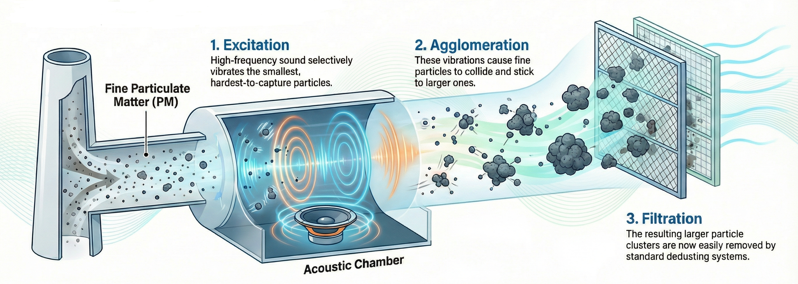
Figure 1.
Schematic concept of the acoustic agglomeration preconditioning of solid particles found in industrial gas emissions.
Figure 1.
Schematic concept of the acoustic agglomeration preconditioning of solid particles found in industrial gas emissions.
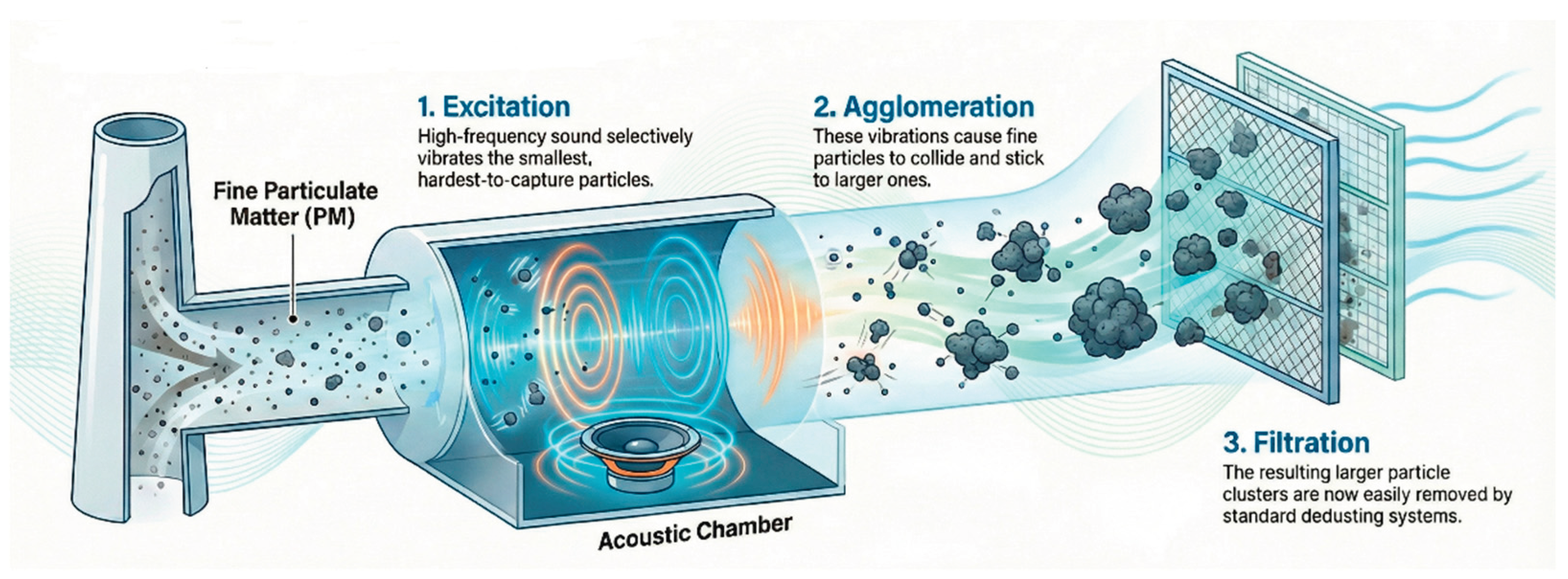
During acoustic agglomeration preconditioning, high-intensity acoustic fields are applied to the flue gas stream, inducing interaction effects among suspended particles, leading to collisions and agglomeration [31]. Testing of this methodology within industrial-scale chambers has demonstrated a potential reduction of up to 70% in the number concentration of micron-sized fly ash particles [32].
The observations and studies of acoustically induced particle interactions have a considerable historical precedent: William Ostwald was the first researcher to suggest as early as 1880 that sound waves could be used as a means to collect small droplets; nevertheless, he did not conduct any acoustic-agglomeration-specific experiments. The earliest documented instance of sound waves affecting droplet size is credited to an anonymous reader of a Norwegian newspaper. This individual observed a disruption in the color pattern of the rainbow during a thunderstorm. The observer theorized that the observed anomaly could be attributed to the acoustic phenomenon of thunder, given the near-simultaneous nature of the events [33]. His assumption was supported later by both theoretical explanations [34] and numerical experiments [35,36].
By the conclusion of the 1920s, independent investigations conducted by researchers Wood and Loomis [37] and Andrade and Lewer [38] yielded a consistent observation: particulate matter subjected to acoustic waves demonstrated a propensity for clustering and aggregation. Subsequently, the phenomenon of acoustic agglomeration became the focus of numerous experimental studies, including those by Patterson and Cawood [39], Andrade [40] and St. Clair [41]. Post-World War II, these investigations were continued in Russia and Poland, resulting in significant contributions by Mednikov [42] and Shirokova [43]. Thereafter, numerous studies, both theoretical and experimental, have been performed on the subject of acoustic agglomeration, targeting the retention of PM from coal-fired ash particles [28,31,32,44,45,46,47,48,49,50,51,52,53,54,55].
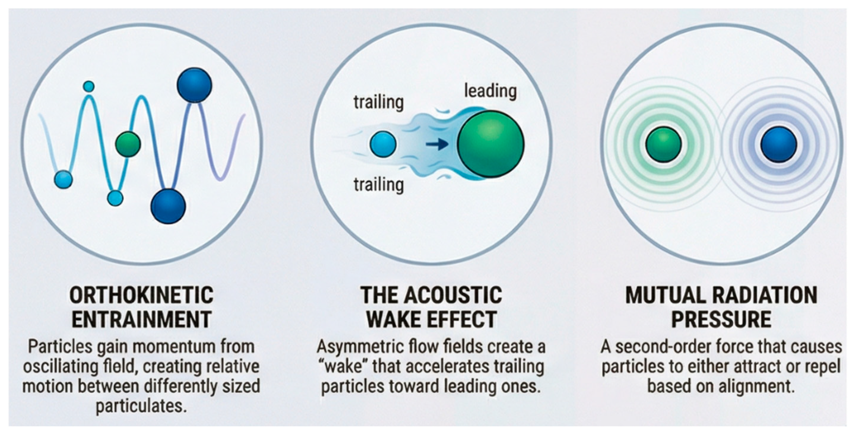
Many physical mechanisms are believed to contribute to the acoustic agglomeration process: the first one to be accounted for is the orthokinetic mechanism, where collisions between particles of different sizes are attributed to the different ways they respond to the acoustic oscillations of the fluid [56]. The variance in particle motion within the acoustic field, described by each particle's entrainment factor, creates a relative velocity that facilitates inter-particle collisions [57]. The orthokinetic mechanism, while considered the primary driver of acoustic agglomeration, fails to account for collisions between particles of uniform size; a phenomenon substantiated by experimental observations [43,58]. Consequently, the hydrodynamic mechanism has been proposed, positing that inter-particle interactions, even among identically sized particles, are induced by hydrodynamic forces generated during close proximity. Two principal hydrodynamic mechanisms are discernible: the first arises from an effect known as the mutual radiation pressure effect (MRPE) and the second from the acoustic wake effect (AWE). In the instance of mutual radiation pressure, hydrodynamic forces known as Bjerknes forces originate from the nonlinear interactions between the particle scattering wave and the incident wave, recognized as secondary acoustic forces [59,60]. Conversely, concerning the acoustic wake effect, the presence of a particle within the asymmetric flow field surrounding another moving particle leads to a decrease in drag force and an acceleration toward the other particle, culminating in their collision over successive acoustic cycles [61]. In addition to the aforementioned primary mechanisms, the literature suggests that particle interactions may be influenced by additional acoustic phenomena such as the primary acoustic radiation force [62], acoustic streaming [63], and acoustic turbulence [64]. However, these influences are considered small relative to orthokinetic and hydrodynamic interactions and are consequently often disregarded in agglomeration studies [65]. All these mechanisms collectively underlie the dynamics of particle convergence and collision. Subsequent to collision, agglomeration ensues due to prevailing attractive forces, specifically van der Waals forces [66].
Numerical modeling and simulation are valuable tools for investigating the influence of various mechanisms on the overall efficiency of acoustic agglomeration in enhancing particle size. The standard approach to numerically analyzing acoustic agglomeration dynamics involves solving the PBE [67] or its discrete form, the Smoluchowski equation [68]. The solution of this equation depicts the temporal evolution of a particle size distribution, contingent upon the accurate definition of the collision rate. It can be solved through deterministic methodologies, such as the method of moments [69], the sectional method [70], the discrete method [71], the discrete-sectional method [72], or stochastic techniques commonly referred to as Monte Carlo (MC) methods [73]. In contrast to deterministic integration, stochastic methodologies employ MC simulations to model the dynamic behavior of a finite ensemble of particles and track their history over time [67].
Figure 2.
Schematic illustrations of the three major acoustic agglomeration mechanisms.
The objective of the present study is to investigate numerically the acoustic agglomeration of liquid particles. Experimental data on glycol fog droplets agglomerated in an acoustic chamber are used to validate the MMC method. A key contribution of this approach is the incorporation of the acoustic wake effect into the agglomeration model employed for the simulations.
2. Methods and Models
The PBE, accounting solely for agglomeration phenomena, is expressed by the following nonlinear integro-differential equation, originally formulated by Friedlander [74]:
where np(υ,t) is the particle size distribution function at time t and β(υ,u) is the agglomeration frequency function of two particles of volumes υ and u. The first term on the right-hand side of Equation (1) is the birth term, accounting for the formation of a particle of volume υ due to an agglomeration event between a particle of volume u and a particle of volume (υ-u). The factor of 1/2 arises from the fact that each agglomeration event involves two particles, necessitating a correction to avoid double counting. The subsequent term represents the attrition of particles with volume υ due to agglomeration with other particles, known as the death term. The third term accounts for particle loss through deposition, as dictated by the deposition kernel, R(υ). The left-hand side of Equation (1) denotes the temporal variation in the number concentration of particles with volume υ. This formulation assumes a spatially homogeneous system, thereby restricting the analysis to the temporal evolution of the particle size distribution function [75]. The term β(υ,u), also referred to as the collision frequency function or kernel, encapsulates the physical mechanisms that drive inter-particle collisions and agglomeration and quantifies the rate at which two particles of volumes υ and u collide. The following sections will provide an overview of prevalent kernels and detail the numerical methodology employed to solve the PBE.
MC methodologies can be categorized into two distinct classes based on the temporal discretization approach: time-driven and event-driven. In time-driven simulations, a predetermined time increment is specified, and all feasible events occurring within this increment are executed. Conversely, event-driven simulations involve the immediate implementation of an event, followed by an adjustment of the simulation time by a corresponding duration [67]. MC methods can be further classified into two primary classes based on the temporal evolution of the simulation volume or the simulation particle number. The first is known as the “constant volume” approach and the second as the “constant number” approach. During the constant volume simulation, the control volume remains invariant despite fluctuations in the number of particles. However, adjustments are made at discrete time intervals when the particle count surpasses or falls below predefined thresholds, thereby ensuring the statistical independence of the solution [73,76]. On the other hand, during the constant number simulation, the number of particles remains constant. Thus, new particles are continuously added or removed from the initial ensemble, contingent on the dynamic process, to uphold the constant particle number [77].
The Multi-Monte Carlo (MMC) methodology, utilized in the present work for the numerical solution of the PBE, was initially developed to reduce computational cost and improve upon the accuracy of the Direct Simulation Monte Carlo (DSMC) method [78]. In addition to operating under a “constant volume and number” regime, the MMC methodology incorporates a “time-driven” approach for time-step management [79]. This time-driven approach entails tracking a simulation particle over a discrete time interval, considering all potential agglomeration events within this period. This consideration is predicated on the assumption that events are independent when the time-step is sufficiently small [80]. A key distinction from the DSMC methodology lies in the representation of simulation entities. Rather than representing individual particles, these entities represent groups of particles with similar properties, referred to as "fictitious" particles. While the concept of fictitious particles has been previously employed in constant number MC methods, the MMC methodology uniquely features a dynamic weight assignment. This weight, denoting the number of real particles represented by a simulation particle, varies in response to prevailing dynamic processes. Specifically, agglomeration reduces the weight and increases the size of simulation particles, whereas deposition only decreases the weight [81].
Within the MMC methodology, the principal stages deal with the determination of each fictitious particle's weight, the establishment of the time step, the identification of a potential agglomeration partner, the evaluation of an agglomeration event incidence, and the subsequent processing of particle agglomeration. Initially, the adjustment of the weight value for each simulation particle is required. Before this adjustment, it is necessary to ascertain the number of discrete size classes that will accurately represent the overall particle distribution, as well as the total number of simulation particles to be employed. Subsequently, the weight of each simulation particle is computed [82]:
(2)
To ensure accurate tracking of all fictitious particles and potential events through appropriate time step selection, it is necessary to avoid the occurrence of multiple events within a single time step. This criterion guarantees the enumeration of each individual event. This stipulation necessitates referencing the dynamic events of actual particles and utilizing kernel information about their frequency. Specifically, the rate of real agglomeration events between particles of the ith-group and the jth-group, per unit time and per unit volume V, is derivable from the equation provided below [78]:
(3)
The agglomeration rate for a representative particle from the ith-group interacting with all other particles can be determined by:
(4)
Consequently, the temporal duration separating two successive agglomeration events of a particle may be expressed as:
(5)
and the time step is calculated as:
(6)
Within the framework of a time-driven methodology such as the MMC, the population evolution is conceptualized as a Markov process [83]. Consequently, the probability of a single agglomeration event occurring for a specific particle belonging to the ith-group during the time interval Δt is given by the following exponential expression:
(7)
To determine whether an agglomeration event occurs for the tracked particle, the Nanbu method will be utilized [84]. Initially, a random number, R1, is generated from a uniform distribution within the interval [0,1). If this number is less than the agglomeration probability mentioned before, an agglomeration event is deemed to have taken place, in accordance with the methodology described by Zhao [85]:
(8)
The subsequent stage in the execution of an individual agglomeration event involves the determination of the agglomeration partner. Given that within the MMC framework, all agglomeration events are defined as binary collisions, only a single partner originating from a jth-group requires selection. For this procedure, the Nanbu method will be utilized again. Initially, the probability of particle i undergoing agglomeration with any other fictitious particle j is calculated as follows [85]:
(9)
The relationship between the agglomeration rate and the agglomeration probability is defined as follows:
(10)
The previously determined random number R1 can be used for the selection of the agglomeration partner. Provided that the subsequent relation is fulfilled, a particle from a jth-group will be selected as the agglomeration partner of the tracked particle of the ith-group:
(11)
After the determination and execution of an agglomeration event, wherein two particles collide and agglomerate into a single larger one, a notable consequence is the progressive reduction of the total number of real particles: smaller particles diminish as larger ones emerge. In the context of the MMC methodology, which involves tracking fictitious particles, the numerical decrease of real particles is reflected through the appropriate adjustment of the weight of the tracked fictitious particles. As a result, the number of fictitious particles remains constant throughout the solution of the PBE, regardless of the quantity of agglomeration events considered or the temporal extent of the PBE's evolution. The operational principle employed in the present work modifies the size and number weight of exclusively one of the coagulating particles, as detailed in [86]:
(12)
(13)
(14)
(15)
Analogously to the treatment of agglomeration events, the determination of whether a deposition event occurs for a fictitious particle i is treated as a Markov process. Consequently, the probability of its deposition within a given time interval Δt is defined by means of the deposition rate R(υ) [81]:
(16)
For a deposition event to be actualized, a new random number, denoted as R2, is drawn from a uniform distribution within the interval [0,1). The deposition will then transpire provided that the following criterion is satisfied:
(17)
Upon the determination of a deposition event, the tracked fictitious particle must be removed from the distribution's particle population. However, this action would inevitably lead to a continuous reduction in particle number, thereby compromising the statistical treatment of the problem, a predicament identical to that encountered during the agglomeration process. To mitigate this issue, a recalibration of the weighting factor is necessary [81]. In the present work, the weight of the tracked particle is set to zero, and the simulation proceeds with this particle included as a "ghost" entity.
3. Agglomeration Kernels
The agglomeration and deposition kernels contain all the information required for modeling a process initiated by a specific physical phenomenon. Particularly for particle agglomeration, these kernels represent the probability of an agglomeration event occurring between two particles. Any mechanism that induces a relative velocity between aerosol particles has an associated agglomeration rate, and thus an agglomeration kernel [87]. The primary mechanisms driving an agglomeration process are Brownian diffusion [74], turbulence-induced motion [88,89], and gravitational settling [90], although any additional process that induces relative motion between particles, such as acoustic forcing, can also promote agglomeration. The kernel employed for solving the PBE is the total agglomeration kernel, which is composed of individual kernels representing the effect of each of the above processes. Each kernel is a function of the sizes of the two particles involved in the collision procedure. In this study, the effects of turbulent and gravitational agglomeration will not be considered since the particles examined are relatively small (micron-sized and sub-micron) and the effects of these mechanisms can be neglected [91].
3.1. Brownian Agglomeration Kernel
The movement of small particles within a quiescent fluid is characterized by the relationship of their size to the mean free path of medium molecules, as described by the Knudsen number, Kn [92]:
(18)
Due to their small size, collisions between these particles and medium molecules result in their random motion (Brownian motion), leading to collisions (thus agglomeration) among the particles themselves. Depending on the value of the Knudsen number (Kn), three particle size regimes are defined: the continuum regime (Kn << 1), the transition regime (1 < Kn < 10), and the free-molecule regime (Kn > 10), and for each regime, a different expression for the collision kernel can be formulated. For the particles examined in the present work, the expression that is valid for the particles in the continuum regime will be used [93]:
(19)
(20)
where kB is the Boltzmann constant, T is the absolute temperature, μ is the dynamic viscosity of the medium, and Cc(υ1), Cc(υ2) are the Cunningham slip correction factors.
3.2. Acoustic Agglomeration Kernel
The orthokinetic and hydrodynamic mechanisms have been identified as the primary contributors to the acoustic agglomeration process. To accurately simulate the impact of each mechanism on the solution of the PBE, a distinct collision kernel must be derived for each one, and the total agglomeration kernel can be expressed as the linear superposition of these kernels:
(21)
where bOI and bHI are the weighting factors of each mechanism’s contribution to the overall kernel. The multiplication factors cannot be theoretically determined. Therefore, a combination satisfying the condition bOI+bHI = 1 can be chosen, or alternatively, values of unity (bOI = bHI = 1) may be adopted, which is the approach employed in the present work.
3.2.1. Orthokinetic Agglomeration Kernel
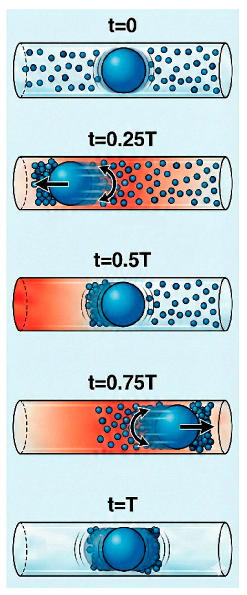
Regarding the orthokinetic mechanism, it is crucial to analyze the oscillatory motion of particles induced by the acoustic wave. Specifically, larger particles tend to remain nearly stationary, whereas smaller particles are almost entirely entrained by the medium, oscillating back and forth with the medium [94]. The concept of the acoustic agglomeration volume was introduced by Mednikov [42] to describe the volume swept by a given particle due to its oscillatory motion (relative to other particles) during a complete acoustic cycle. Initially, large particles (collectors) are located at the center of the agglomeration volume, while small particles are distributed uniformly throughout. During a quarter of the acoustic wave period, larger particles move to the left side of the agglomeration volume relative to smaller particles, consequently capturing them. At t = 0.5T, the large particles return to the center of the agglomeration volume. During the subsequent quarter-cycle, the larger particles migrate toward the opposite side of the agglomeration volume, collecting smaller particles. At t = T, the oscillating medium conveys the larger particles back to their initial position. Mednikov’s main assumption was that all particles within the agglomeration volume are captured and that this volume is entirely replenished by other particles within a single acoustic cycle. Considering only two types of particles (1 is the oscillating collector and 2 are the particles that are inside the agglomeration volume), then the agglomeration kernel for this mechanism can be expressed as follows (Mednikov formulation):
(22)
where d1 and d2 represent the particle diameters, U0 denotes the velocity amplitude of the sound wave, and n12 is the relative entrainment factor between the two particles:
(23)
Figure 3.
Schematic illustration of the acoustic agglomeration volume.
In the above equation, the H-function is the ratio of the complex velocity amplitude of the particle Up to that of the fluid medium U0 [95]:
(24)
(25)
where λp is the ratio of the fluid density, ρf, to the particle density, ρp, ω is the angular frequency of the acoustic wave, and δv is the penetration depth of the viscous wave [96]:
(26)
The magnitude and phase of the H-function are respectively the entrainment factor and phase delay of the particle [97]:
(27)
(28)
(29)
The expression for the relative entrainment factor n12 can now be written as:
(30)
A major limitation of the Mednikov model is that the oscillatory motion of particles and the mutual scattering interactions between them are not considered in the derivation of the agglomeration volume [98]. Later, Song included them in his study and modified the Mednikov expression by introducing a new formulation for the relative entrainment factor of two particles [65]:
(31)
where G12 is the so-called scattering interaction function and a detailed description can be found in Song’s dissertation.
3.2.2. Hydrodynamic Agglomeration Kernel
Apart from the linear particle-gas interactions inherent in the orthokinetic mechanism, nonlinear inter-particle interactions also occur within an oscillating gas [99]. These interactions can be attributed to either nonlinear interactions between particle scattering waves and the incident field, termed the MRPE [100], or to viscous asymmetries in the flow field surrounding the particles, leading to the AWE [101]. To investigate the influence of these interactions on particle motion, it is necessary to calculate the forces exerted on particles in the Stokes flow regime (giving rise to Bjerknes or König forces) and in the Oseen flow regime. Bjerknes forces are derived from Bernoulli's hydrodynamic principle and are applicable for arbitrary particle orientations. Conversely, Oseen hydrodynamic forces arise from the viscous asymmetry of the flow field around oscillating particles. Both force types act concurrently on particles exposed to an acoustic field; however, distinct agglomeration kernels have been formulated for each to facilitate further investigation into their impact on the acoustic agglomeration process.
3.2.2.1. Mutual Radiation Pressure Effect Kernel
The proximity of two moving particles within an acoustic field induces additional scattered waves that interfere with their trajectories. The nonlinear interaction between the incident wave and the waves scattered by each particle generates a resultant wave, disturbing nearby particles and influencing their motion. The non-uniform spatial distribution of scattering velocity leads to a net pressure force between the particles [59,102]. These forces, stemming from viscous interactions between particles and the surrounding fluid, are commonly referred to as secondary acoustic forces [103]. Such forces can result in either attraction or repulsion between proximate particles, depending on the orientation of the lines connecting the particles’ centers and the acoustic vector [91]. These forces induce a relative velocity that may culminate in collision and subsequent agglomeration [59]. In an ideal fluid, the influence of secondary acoustic forces on particle motion is considerably less significant than that of the particle's penetration into the acoustic field, leading Mednikov to disregard them [104]. Nevertheless, when particle size diminishes (consequently intensifying the effect of viscosity) or when the acoustic field is intense (at a minimum, approximately 160 dB), it becomes necessary to consider these forces and incorporate their action into the acoustic agglomeration process by formulating the corresponding agglomeration kernel.
For this hydrodynamic mechanism, the agglomeration frequency function can be described by the classic expression of König, whose calculation of the forces between two particles was based on the Bernoulli effect. König's expression for the collision kernel takes the form:
(32)
Danilov and Mironov [105] were the first to incorporate the viscous effects on such Bernoulli interactions and formulated an overall approach for the Bjerknes forces. Later, Song extended their work by also incorporating the effect of particle entrainment and the separation distance between particles, and formulated the following expression for the hydrodynamic mechanism [65]:
(33)
The parameter g12, a complex algebraic expression known as the hydrodynamic interaction function, accounts for the effects of entrainment and scattering waves; a detailed derivation can be found in Song's dissertation [65].
3.2.2.2. Acoustic Wake Effect Kernel
An asymmetry in the flow field surrounding a particle undergoing oscillatory motion in an acoustic field generates a wake characterized by an area of reduced pressure downstream of the particle. This phenomenon (acoustic wake effect) manifests under specific flow conditions, notably the Oseen flow regime, i.e., a moderate Reynolds number [106]. The presence of a proximate oscillating particle within the wake of a leading particle results in a reduction of drag, causing it to move towards the leading particle. These interacting particles exhibit mutual perturbation of their trajectories due to their periodically varying wakes [107]. Mathematical formulations for their convergent velocity in Oseen flow fields were initially developed for particles of identical size by Pshenai-Severin [101] and subsequently extended to particles of differing sizes by Dianov [108].
Though the acoustic wake effect is a purely hydrodynamic mechanism, its associated collision kernel can be expressed by considering it as a refill mechanism for the acoustic agglomeration volume, which was previously used to formulate the orthokinetic agglomeration kernel. In Mednikov's classical theory, after one acoustic cycle, all particles are swept by the core oscillating particle, and the emptied agglomeration volume is assumed to be automatically refilled by smaller particles with an arbitrarily set unity refill factor [109]. However, if physical mechanisms such as gravity, acoustic wave scattering, mutual radiation pressure, acoustic streaming, or the acoustic wake effect are considered as refill mechanisms, the volume will only be partially refilled. If the acoustic wake is considered the primary refill mechanism, the agglomeration kernel can be calculated as follows [61]:
(34)
The refill factor R12 has been calculated as an extension to the length of the acoustic agglomeration volume formulated by Mednikov, L21:
(35)
where l1 and l2 are the particle slip coefficients in the Oseen regime [108] and Tac is the acoustic period. The length L21 can be calculated from the relative displacement between the particles [109]:
(36)
In this equation, x1 and x2 are the particle displacement amplitudes and LAWE is the acoustic wake volume length that can be calculated as follows [61]:
(37)
4. Results and Discussion
To investigate the influence of acoustic agglomeration on particle size distribution, a representative cell containing up to 4 × 10¹² real particles/m3 is isolated from an aerosol system and used in the simulation. Unless specified otherwise, the simulation is conducted with N0 = 9,000 fictitious particles, and the size distribution is discretized into 500 logarithmically spaced bins within the range of 0.1 μm–500 μm. For the purpose of simulation validation, the MMC model will first be compared against experimental data (accounting for both Brownian motion and acoustic agglomeration) and subsequently against numerical results obtained by other researchers, based on the same experimental dataset.
The experimental data employed pertain to the temporal evolution of an initial aerosol mixture subjected to an acoustic field. These data were originally documented in the work of J. Magill [110] and further elaborated upon by P. Caperan and J. Somers [111,112], who built upon Magill's original research. These experiments investigated the time-dependent evolution of a distribution of liquid glycol particles under the influence of an acoustic field with varying intensity and frequency. All studies mentioned above utilized a standard experimental configuration. This setup comprised an agglomeration chamber for introducing the aerosol mixture, a sound source connected to a piezoelectric transducer for generating the acoustic field, and the requisite instrumentation for monitoring the particle distribution over time. The sound source is capable of operating at different frequencies and is supplied with electrical power, which can be correlated with various acoustic velocity amplitudes (as detailed in Table 1). These amplitudes were calculated using charts, provided by Caperan and Somers, that convert electrical power to acoustic pressure. Magill, in his experimental study of agglomeration, employed an acoustic chamber in the form of a 0.6 m³ acrylic glass/PMMA container. In contrast, Caperan and Somers provide a more detailed description of a slightly larger cylindrical container, measuring 2 m in length and 0.7 m in diameter. A key distinction between the two setups is that Caperan and Somers incorporated a layer of absorbent material at one end of their chamber to simulate the effect of a traveling acoustic wave on the particle mixture. Both initial mixtures are assumed to follow a log-normal distribution, with their characteristics presented in Table 1.
In addition to the experimental data, results from the work of O. Ezekoye and Y. Wibowo [59] and C. Sheng and X. Shen [113] are employed. Both studies numerically investigated the same instances of acoustic agglomeration. The former utilized a modified numerical model of Gelbard and Seinfeld’s sectional code MAEROS [114], whereas the latter solved the problem stochastically using the DSMC methodology. These findings will also serve as a foundation for validating the proper functioning of the MMC methodology in modeling acoustic agglomeration, particularly concerning the form of the agglomeration kernel, as such information cannot be gleaned from experimental results.
The liquid nature of the aerosol particles (droplets) implies that their agglomeration results in the formation of larger spherical particles of uniform density. This characteristic substantially simplifies the simulation, as all kernel expressions for spherical particles remain applicable. Furthermore, a simplifying assumption in the numerical calculations is that every collision event results in agglomeration, thus setting the collision efficiency to unity [115]. Additionally, the computational code inherently assumes spatially homogeneous conditions for both particle number concentration and the acoustic field. This necessitates a traveling wave acoustic field, a condition adopted in other simulation studies [59], and a uniform particle distribution throughout the entire field (a homogeneous mixture, facilitated by a fan within the acoustic agglomeration chamber). Lastly, as noted by Caperan and Somers, other phenomena stemming from the sound's influence on the fluid, such as acoustic streaming or acoustic turbulence, as well as the effect of the primary acoustic force, are of negligible intensity and are therefore excluded from the calculations [112].
Figure 4 compares the strengths of various agglomeration mechanisms examined in the present work. The graph pertains to a scenario where one particle has a diameter of 1 μm, the sound intensity is 100 W, and the acoustic frequencies are 10 kHz and 21 kHz. The size of the second particle ranges from 0.1 μm to 50 μm. The kernel's intensity directly correlates with its contribution to the overall agglomeration process. This figure clearly shows that acoustic mechanisms (both orthokinetic and hydrodynamic) contribute significantly more than the Brownian mechanism, with their intensity nearly two orders of magnitude higher. As anticipated, the Mednikov approach exhibits the highest intensity, which is attributable to its assumptions of an ideal fluid and complete volume refilling after a single acoustic cycle. This overestimation of the agglomeration rate will subsequently be demonstrated through comparison with experimental data. Conversely, Song’s mechanism, which incorporates the effect of scattering waves that reduce the number of particles within the agglomeration volume, is considerably weaker. Further observation of these curves reveals that the orthokinetic mechanism, in both its formulations, asymptotically approaches zero when the two particles are of identical size. This outcome aligns with its algebraic expression, as identically sized particles oscillate in the same manner within the sound field, precluding the development of relative velocity.
On the other hand, the hydrodynamic mechanism exhibits nearly constant growth with increasing particle size, and for particles of identical size, the kernel does not reach zero. This accounts for the experimentally observed agglomeration of similarly sized particles. Nevertheless, employing Song’s expression for this mechanism reveals a behavior similar to the orthokinetic mechanism, albeit less pronounced. This resemblance is anticipated, given Song's inclusion of particle entrainment in his formulation. Furthermore, with the incorporation of viscosity and the influence of scattering waves, the hydrodynamic mechanism can become comparable to the orthokinetic mechanism, potentially exerting a more significant impact on the agglomeration process.
Additionally, the expression for the kernel used to describe the acoustic wake effect is plotted in Figure 4. Since this kernel was derived as a correction to the Mednikov expression, a similar order of magnitude is anticipated. However, for equally sized particles, a reversed trend relative to the orthokinetic mechanism is observed, as the number of collisions is not diminished. This is attributed to the fact that the convergent velocity between the two particles, when calculated using the acoustic wake effect theory, is not zero for particles of the same size. From this figure, it is also evident that this mechanism is stronger than the MRPE, which is consistent with experimental observations of particle trajectories of similar size under acoustic conditions in the Oseen flow regime [116,117].
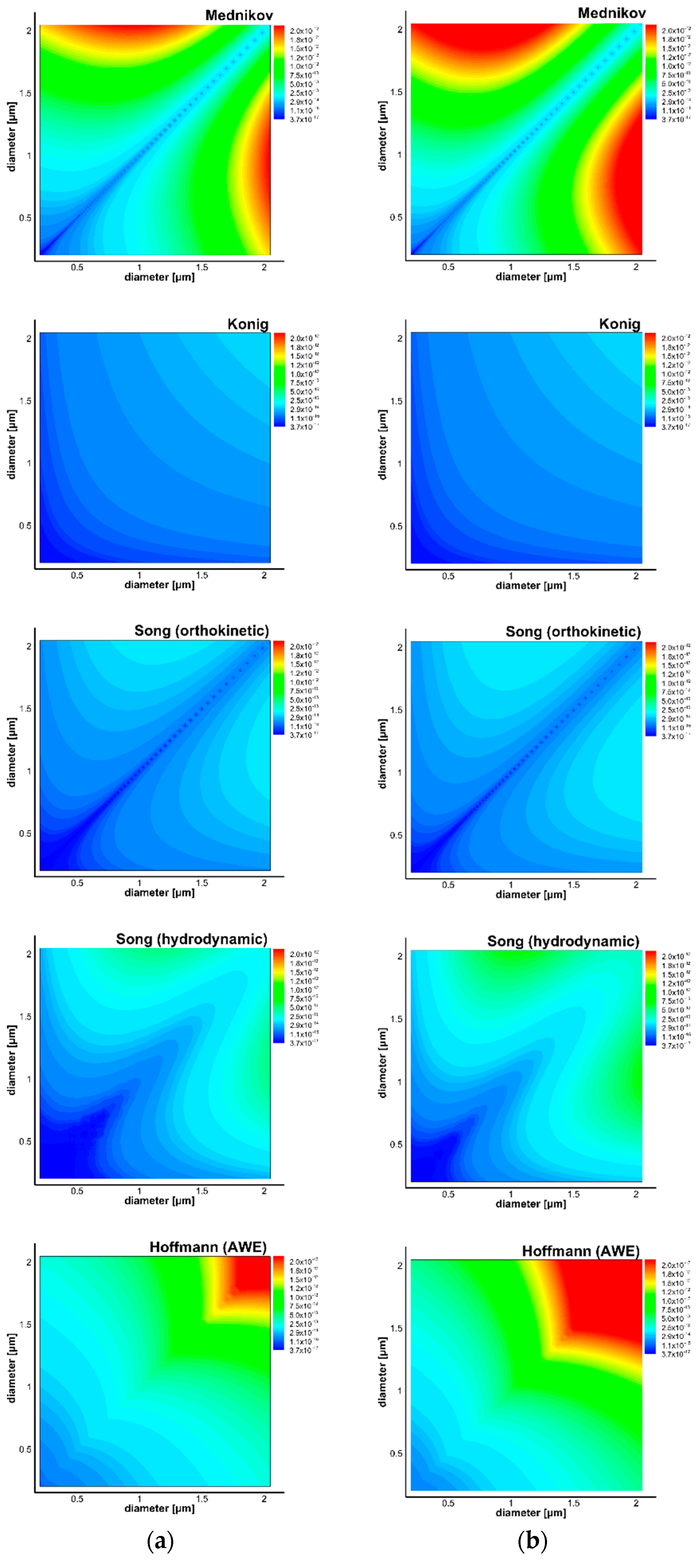
Figure 5.
Contour plots illustrating the intensity of the various acoustic agglomeration mechanisms for different pairs of particle diameters. The collision frequency is expressed in units of m3/s, and acoustic velocity amplitude U0 = 0.98 m/s with a sound frequency of (a) 10 kHz; (b) 21 kHz.
Figure 5.
Contour plots illustrating the intensity of the various acoustic agglomeration mechanisms for different pairs of particle diameters. The collision frequency is expressed in units of m3/s, and acoustic velocity amplitude U0 = 0.98 m/s with a sound frequency of (a) 10 kHz; (b) 21 kHz.
Initially, the outcomes of the MMC model, considering only Brownian motion as the agglomeration mechanism, will be presented. To monitor the temporal evolution of the agglomeration process, the non-dimensional particle number concentration, expressed as N/N0 (where N0 represents the initial total particle number concentration), will be depicted as a function of time. Experimental data from Caperan [112] and numerical simulation results from Sheng's DSMC method will be utilized [113]. As shown in Figure 6, both numerical simulations yield nearly identical results but underestimate the particle number concentration reduction compared to the experimental results. This discrepancy may be attributable to either the deposition of particles on the chamber walls or the gravitational sedimentation of particles. Inclusion of deposition effects in the simulation demonstrates an increased particle removal rate, aligning more closely with experimental observations. However, to ensure direct comparability with other simulation efforts, subsequent results of the acoustic agglomeration processes will exclude the influence of the deposition mechanism.
4.1. Influence of Agglomeration Kernel Expression and Residence Time
Figure 7 and Figure 8 display the temporal evolution of the non-dimensional particle number concentration, incorporating the effect of acoustic agglomeration in the simulation. A variety of individual kernels were examined, considering two distinct acoustic field frequencies at one fixed sound intensity (100 W). The combination of two kernels was performed using a simple additive method with unity multiplication factors, as previously described. In all numerical attempts, the influence of the Brownian kernel was included, but the deposition mechanism was neglected. The results from both the DSMC and MMC simulations are presented alongside the experimental data from Caperan et al. [112]. Regarding the validity of the MMC simulation, both numerical simulations predict nearly identical effects of the acoustic agglomeration process for each combination of mechanisms employed, a result that was anticipated given the nature of the two methodologies (both are statistical). A discrepancy is observed in the results of these two methodologies when the Song hydrodynamic mechanism is utilized, but this deviation is minor (4%–5% of the total range) and may be attributed to uncertainties in the formulation of the hydrodynamic interaction function employed in the DSMC. These figures illustrate that the total particle number concentration decreases over time; this decrease is significantly influenced by the acoustic field rather than by Brownian motion alone. The total number concentration is observed to decrease monotonically as the residence time increases. Nevertheless, the effect of agglomeration is more pronounced during the initial stages of the acoustic treatment compared to later periods.
The choice of kernel expressions significantly influences the simulation outcomes. For the orthokinetic mechanism, the Mednikov formulation consistently overestimates the agglomeration rate. This is because it assumes the agglomeration volume is completely refilled with particles after one acoustic cycle. In contrast, Song's approach refines Mednikov's formulation by incorporating both scattering effects and the oscillatory motion of the particle. These factors reduce the number of particles that refill the agglomeration volume, leading to fewer inter-particle collisions and, consequently, a smaller decrease in the particle number concentration. Regarding the hydrodynamic mechanism, the König formulation underestimates the experimentally observed reduction in particle number concentration, because the ideal fluid assumption neglects viscous effects, which, according to Song, could lead to an increase in the strength of the agglomeration kernel by up to eight orders of magnitude [65]. When these effects are incorporated (via Song's expression), the reduction in particle number concentration is overestimated, particularly during the initial stages of the simulation for both methodologies. However, within the context of the MMC simulation, a better agreement with the experimental results is observed during the later stages of the agglomeration process, especially for the low-frequency case.
Should the kernel expression based on the AWE be employed for the simulation, the reduction in particle number concentration is comparable to, though smaller than, the one predicted using the Mednikov approach. This is expected, as this formulation is derived from the Mednikov approach but incorporates a refill mechanism for the agglomeration volume that does not take unity values. For both cases investigated (10 kHz and 21 kHz), the results exhibit closer agreement with the experimental data. Furthermore, for the higher frequency case, the deviation from the Mednikov simulated results is less pronounced than for the lower frequency case.
Figure 9 compares the particle size distribution after acoustic agglomeration as predicted by the present model and the numerical simulation utilizing the DSMC. For this comparison, an acoustic treatment of 400 s was selected, and two distinct scenarios were analyzed: first, employing only Song's orthokinetic mechanism, and subsequently, incorporating the hydrodynamic mechanism via the König expression. The results confirm the formation of larger particles at the expense of smaller ones. Furthermore, the acoustic treatment shifts the particle distribution from a log-normal to a bimodal form, an observation consistent with acoustic agglomeration experiments conducted by other researchers [57]. When the hydrodynamic mechanism is included in the simulation, the distribution curve exhibits a flatter profile toward the higher end, leading to the creation of larger particles within the same acoustic treatment duration compared to the exclusive action of the orthokinetic mechanism. This outcome is attributed to the hydrodynamic mechanism promoting collisions between larger, similarly sized particles, which subsequently act as efficient capturers for smaller ones.
To further examine the temporal evolution of the particle distribution characteristics during the numerical simulation, the mean mass and number diameters of the particle size distribution are presented as a function of time in Figure 10. For both kernel configurations, the mass mean diameter consistently increases, indicating the formation of larger particles. When both kernels are utilized, the rate of increase is steeper. As previously explained, this is attributed to the hydrodynamic mechanism, which favors the agglomeration of particles of similar, larger sizes, while the orthokinetic mechanism promotes the agglomeration of particles with large size differences. This trend is also evident in the time evolution of the number mean diameter presented in Figure 10: since the newly created larger particles are fewer in number, their formation leads to a reduction in the number mean diameter from a certain time onwards.
4.2. Influence of Sound Field Intensity
Figure 11 illustrates the numerically predicted particle number concentration following acoustic agglomeration at various acoustic intensities. Greater acoustic intensity corresponds to an increased gas velocity, and consequently, more intense relative motion between the particles. As anticipated, the sound intensity directly influences the acoustic agglomeration results: a stronger sound field leads to a larger increase in acoustic agglomeration efficiency. This relationship is also evident from the relevant kernel expressions: the orthokinetic mechanism is directly proportional to the acoustic wave amplitude U0, while the hydrodynamic mechanism exhibits a quadratic dependence. This figure employs the combined Song’s and König’s formulation for the orthokinetic and hydrodynamic mechanisms.
In Figure 12, a comparison is presented between the numerical simulation results for acoustic agglomeration and the experimental data reported by Magill and Caperan, considering Song's hydrodynamic expression in the numerical model. The convergence between the two numerical methodologies is again observed; however, a divergence from the experimental data is apparent across all examined cases, in which Song's expression for the hydrodynamic mechanism serves as the agglomeration kernel.
The divergence of the results of both numerical methodologies from the experimental data may be attributable not only to the algebraic form of the kernel but also to other factors affecting particle number concentration, such as the deposition or breakup of aggregates in high-intensity acoustic environments [118], which have not been included in the modeling. Furthermore, other phenomena that may enhance the agglomeration process but have not been modeled through the previously presented kernels are of particular interest: one of these is acoustic turbulence caused by the propagation of high-intensity sound fields. This phenomenon can also trigger particle collisions, thereby increasing the efficiency of acoustic agglomeration [119]. It has been observed experimentally that for sound field intensities exceeding 158 dB, this kind of turbulence appears, while for intensities greater than 160 dB, even shock waves can be generated in the medium when the sound is propagating [120]. Figure 13 presents the results obtained when utilizing the acoustic wake kernel as the exclusive agglomeration mechanism. For both simulated sound frequencies, the influence of the acoustic field's intensity is observed to be consistent with the previously studied mechanisms; specifically, a higher intensity correlates with a greater reduction in the particle number concentration.
4.3. Influence of Initial Particle Number Concentration and Shape of Distribution
The initial particle number concentration, N0, constitutes a fundamental parameter influencing acoustic agglomeration, as is the case for all agglomeration processes. A higher initial particle number density serves to accelerate the rate of agglomeration. Regarding the orthokinetic mechanism, the reduction in initial inter-particle distance (resulting from increased concentration) enhances its effectiveness, as a greater number of particles are positioned within the agglomeration volume. Likewise, the hydrodynamic mechanism is intensified; since it is inversely proportional to the distance between particle centers, a reduction in this distance leads to a more pronounced interaction. Figure 14 shows the temporal evolution of particle number concentration within a specific acoustic field across six distinct cases of initial concentration. As evidenced by the slope of the individual curves, the agglomeration process intensifies as the initial particle count increases, a trend validated by both experimental data and corresponding numerical simulations. This behavior is consistent with experimental studies on acoustic agglomeration conducted by other researchers [31,110,121]. However, other experimental records indicate that beyond a certain threshold, an increase in particle number concentration may lead to a regime in which the agglomeration process is attenuated. This occurs due to the absorption of the acoustic field intensity by the particle mixture itself [122], a phenomenon that is not accounted for in the present study.
The initial shape of the particle size distribution also influences the acoustic agglomeration process. For this reason, numerical simulations were conducted for two additional different forms of the initial distribution: in the first case, the mean diameter was increased (keeping the number of particles and standard deviation fixed), while in the second case, the geometric standard deviation was varied (keeping the mean value and number of particles the same). This influence is best illustrated by examining the intersection of the particle cumulative size distribution curve and the acoustic particle entrainment coefficient curve, for two different acoustic frequencies, as shown in Figure 15. When the distribution is shifted toward larger particles, it is evident that more particles will acquire high relative velocities, which is expected to favor the agglomeration process insofar as the orthokinetic mechanism is concerned. On the other hand, a distribution with a large initial standard deviation spans a wider range of particle sizes, since the distribution curve (bell curve) is broader. Regarding the action of the hydrodynamic mechanism, this is also favored by the presence of larger particles, as the resulting hydrodynamic force is proportional to their size.
Figure 16 shows the results of the numerical simulation when the combination of Song’s orthokinetic formulation and König’s hydrodynamic formulation is used. The acoustic treatment was considered for a duration of 50 s, incorporating two distinct sound frequencies. It is evident that an increase in the mean diameter of the initial particle size distribution exerts a more substantial influence on the acoustic agglomeration than an increase in the geometric standard deviation.
4.4. Influence of Particle Density
Particle density is also a critical factor influencing acoustic agglomeration, as its value dictates the behavior within the acoustic field. Specifically, heavier particles (with a longer relaxation time) exhibit a slower response to fluctuations in the acoustic field, leading to a reduction in their entrainment coefficient. By plotting the entrainment coefficient for two distinct particle densities across two different acoustic frequencies (as illustrated in Figure 17), it is observed — again through the intersection of these curves — that heavier particles result in a larger population acquiring high relative velocities. Increased particle density enhances acoustic agglomeration, primarily through the orthokinetic mechanism. Conversely, the hydrodynamic mechanism remains unaffected by particle density, being solely dependent on particle diameter. This is because the driving force for the hydrodynamic mechanism, namely secondary acoustic forces, is exclusively governed by the asymmetry of the flow field surrounding the particle. Therefore, the decrease in particle number concentration is more pronounced for these heavier particles than for lighter ones, particularly during the later stages of the agglomeration process where larger particles are formed.
The predicted size distributions of particles of two different densities after 100 s of acoustic treatment are presented in Figure 18. It seems that for the heavier particles, the number reduction is more pronounced (in the range 0.1 μm–2 μm) for both acoustic frequencies examined.
4.5. Influence of Sound Frequency
Frequency is also a critical parameter influencing both the orthokinetic and hydrodynamic mechanisms. The preceding experimental results and numerical simulations indicate that a higher acoustic field frequency promotes agglomeration of the aerosol mixture. However, the influence of frequency on the evolution of the particle size distribution remains unclear upon initial consideration. Acoustic agglomeration investigations have spanned a broad spectrum of acoustic frequencies, ranging from the low values of 44 Hz [31] and 3 kHz [121], to the high-frequency fields of 10 kHz and 21 kHz [112,123]. While low-frequency sound sources were historically favored due to their cost-effectiveness and reliability, substantial advancements have recently been made in the development of devices capable of producing high-frequency and high-intensity acoustic fields. These innovations are primarily relevant for the industrial application of acoustic agglomeration [98].
To gain a deeper understanding of how frequency influences the action of each mechanism, one must examine its effect on the underlying driving force. It should be noted that, as demonstrated by the relevant equation, König's expression for the hydrodynamic kernel is solely dependent on the acoustic velocity amplitude and not on the sound frequency. This observation stems from the assumption that the fluid is considered ideal and that the particles are significantly smaller than the sound field wavelength. Only when accounting for viscous effects (i.e., wave scattering) and particle entrainment, as incorporated by Song into his expression for the hydrodynamic mechanism, does the frequency exert an influence on the corresponding collision kernel. Figure 19 illustrates the effect of frequency on the acoustic entrainment factor and the hydrodynamic interaction function g12. From this figure, it is observed that the entrainment factor of a particle of a given diameter decreases with increasing sound frequency, indicating a reduction in the particle vibration speed. However, since the orthokinetic mechanism is directly related to the relative velocity of two particles, an optimal frequency exists, determined by the initial particle distribution, that promotes collisions. This is why the cumulative particle size distribution is also plotted in Figure 19. When the sound frequency is very low (~1 kHz), all particles are equally entrained by the acoustic waves (unity entrainment coefficient), resulting in minimal relative motion and thus few collisions. Conversely, when a higher frequency is selected (>20 kHz), a range of particle sizes exists where the entrainment factor transitions from unity (fully entrained) to a lower value. Particles of different sizes within this range will experience varying entrainment rates, thereby enhancing the probability of agglomeration.
Regarding the influence of the sound frequency on the effect of the scattering waves on the hydrodynamic mechanism, the most important property of this interaction between two particles is that these hydrodynamic forces depend on the source strength of these waves, which, in turn, is dependent on the product of (1−H1) and (1−H2) instead of the difference (H1−H2) [98,124]. Consequently, if H1 and H2 are smaller in magnitude, the hydrodynamic forces will be larger. This indicates that a higher sound frequency corresponds to stronger hydrodynamic interaction. Conversely, for very small particles or low frequencies, the entrainment factor approaches unity, resulting in these strengths being close to zero and the scattered waves being weak [124]. Furthermore, in the case of two particles of identical size, the term simplifies to (1−H)2, which remains non-zero as long as the particles are not fully entrained. Thus, higher frequencies will also favor the development of relative motion based on the radiation pressure interaction and promote particle collisions. Additionally, higher frequencies result in a greater flow-around velocity, which enhances the distortion of the flow field and consequently increases the agglomeration kernel of hydrodynamic interaction [125].
Regarding the influence of sound frequency on the AWE (as investigated by Hoffmann [61]), the extended length of the agglomeration volume increases with higher frequencies, asymptotically approaching a constant value for any given pair of particles. Figure 20 illustrates the effect of sound frequency on the AWE kernel, alongside the corresponding Mednikov formulation. Since the AWE was conceptualized by Hoffmann as a variation of the Mednikov expression, a similar trend is observed when considering a pair of particles, where one particle has a fixed diameter of 1 μm and the other ranges from 0.1 μm to 10 μm. Fundamentally, increasing the sound frequency consistently enhances agglomeration [126].
Figure 21 illustrates the numerical simulation results regarding particle number concentration and the predicted particle size distribution after 100 s of acoustic treatment across four distinct acoustic frequencies. The utilized kernel combines Song's orthokinetic mechanism with König's hydrodynamic mechanism. Higher frequencies lead to a reduction in particle number concentration and broader distribution shapes, indicating the formation of larger particles at the expense of smaller ones.
5. Conclusions
The present study employs the Multi-Monte Carlo (MMC) method to solve the population balance equation (PBE) while accounting for particle acoustic agglomeration. The MMC technique utilizes the concept of "weighted fictitious particles" whose number is significantly smaller than the actual number of particles. The MMC method has been successfully applied to simulate various acoustic treatment scenarios using different agglomeration kernels. The agglomeration kernel incorporated models for orthokinetic and hydrodynamic mechanisms, as well as Brownian agglomeration and particle deposition. Furthermore, the contribution of the acoustic wake effect to the agglomeration process was evaluated. The results obtained from the MMC method exhibit good agreement with other numerical approaches such as Direct Simulation Monte Carlo (DSMC) and the sectional method (MAEROS), and available experimental results, thereby validating the computational precision and reliability of the MMC approach. A parametric examination investigated the influence of key parameters, such as sound frequency and intensity, along with initial particle size distribution characteristics, with the objective of numerically simulating the acoustic treatment of liquid aerosols. Sound frequency was identified as a critical parameter in controlling the particle size distribution and the number concentration of the treated aerosol. However, the optimal selection of this value requires joint consideration of the initial particle size distribution.
In summary, acoustically driven agglomeration leads to a diminished number density of fine particles and the subsequent emergence of larger counterparts. The proposed MMC methodology provides a rapid simulation tool for understanding and optimizing the acoustic agglomeration process.
Funding
This research has received partial financial support from the “Greek State Scholarships Foundation / IKY”.
Institutional Review Board Statement
Not applicable.
Informed Consent Statement
Not applicable.
Data Availability Statement
No new data were created in this study.
Acknowledgments
During the preparation of this manuscript/study, the authors used Google NotebookLM for the purpose of creating schematic graphs. The authors have reviewed and edited the output and take full responsibility for the content of this publication.
Conflicts of Interest
The authors declare no conflicts of interest.
Abbreviations
The following abbreviations are used in this manuscript:
| AQG | Air Quality Guidelines |
| AWE | acoustic wake effect |
| DSMC | Direct Simulation Monte Carlo |
| EPA | Environmental Protection Agency |
| MC | Monte Carlo |
| MMC | Multi-Monte Carlo |
| MRPE | mutual radiation pressure effect |
| PAHs | polycyclic aromatic hydrocarbons |
| PM | particulate matter |
| PBE | Population Balance Equation |
| WHO | World Health Organization |
References
- Balakrishnan, V.S. Clean Air, Climate Targets, and Respiratory Health in Europe. Lancet Respir. Med. 2025, 13, e12–e13. [Google Scholar] [CrossRef]
- Grantz, D.A.; Garner, J.H.B.; Johnson, D.W. Ecological Effects of Particulate Matter. Environ. Int. 2003, 29, 213–239. [Google Scholar] [CrossRef]
- Thangavel, P.; Park, D.; Lee, Y.-C. Recent Insights into Particulate Matter (PM2.5)-Mediated Toxicity in Humans: An Overview. Int. J. Environ. Res. Public Health 2022, 19, 7511. [Google Scholar] [CrossRef]
- Atkinson, R.W.; Kang, S.; Anderson, H.R.; Mills, I.C.; Walton, H.A. Epidemiological Time Series Studies of PM2.5 and Daily Mortality and Hospital Admissions: A Systematic Review and Meta-Analysis. Thorax 2014, 69, 660–665. [Google Scholar] [CrossRef] [PubMed]
- Lippmann, M. Toxicological and Epidemiological Studies of Cardiovascular Effects of Ambient Air Fine Particulate Matter (PM2.5) and Its Chemical Components: Coherence and Public Health Implications. Crit. Rev. Toxicol. 2014, 44, 299–347. [Google Scholar] [CrossRef]
- Park, M.; Joo, H.S.; Lee, K.; Jang, M.; Kim, S.D.; Kim, I.; Borlaza, L.J.S.; Lim, H.; Shin, H.; Chung, K.H.; et al. Differential Toxicities of Fine Particulate Matters from Various Sources. Sci. Rep. 2018, 8, 17007. [Google Scholar] [CrossRef] [PubMed]
- Manisalidis, I.; Stavropoulou, E.; Stavropoulos, A.; Bezirtzoglou, E. Environmental and Health Impacts of Air Pollution: A Review. Front. Public Health 2020, 8, 14. [Google Scholar] [CrossRef]
- World Health Organization. WHO Global Air Quality Guidelines: Particulate Matter (PM2.5 and PM10), Ozone, Nitrogen Dioxide, Sulfur Dioxide and Carbon Monoxide; World Health Organization: Genève, Switzerland, 2021; ISBN 9789240034228. [Google Scholar]
- Pai, S.J.; Carter, T.S.; Heald, C.L.; Kroll, J.H. Updated World Health Organization Air Quality Guidelines Highlight the Importance of Non-Anthropogenic PM2.5. Environ. Sci. Technol. Lett. 2022, 9, 501–506. [Google Scholar] [CrossRef]
- Wooley, D.; Leiter, A.; Salgado, M.; Zalzal, P. EPA’s New Particulate Matter Standard. Env’t L. Rep. 2024, 54, 10535. [Google Scholar]
- Martins, N.R.; Carrilho da Graça, G. Impact of PM2.5 in Indoor Urban Environments: A Review. Sustain. Cities Soc. 2018, 42, 259–275. [Google Scholar] [CrossRef]
- Li, C.; Managi, S. Contribution of On-Road Transportation to PM2.5. Sci. Rep. 2021, 11, 21320. [Google Scholar] [CrossRef]
- Buonocore, J.J.; Dong, X.; Spengler, J.D.; Fu, J.S.; Levy, J.I. Using the Community Multiscale Air Quality (CMAQ) Model to Estimate Public Health Impacts of PM2.5 from Individual Power Plants. Environ. Int. 2014, 68, 200–208. [Google Scholar] [CrossRef] [PubMed]
- Gao, M.; Liang, C.; Hong, W.; Yu, X.; Zhou, Y.; Sun, R.; Li, H.; Huang, H.; Gan, X.; Yuan, Z.; et al. Biomass-Related PM2.5 Induces Mitochondrial Fragmentation and Dysfunction in Human Airway Epithelial Cells. Environ. Pollut. 2022, 292, 118464. [Google Scholar] [CrossRef]
- Azarmi, F.; Kumar, P.; Marsh, D.; Fuller, G. Assessment of the Long-Term Impacts of PM10 and PM2.5 Particles from Construction Works on Surrounding Areas. Environ. Sci. Process. Impacts 2016, 18, 208–221. [Google Scholar] [CrossRef]
- Roberts, G.; Wooster, M.J. Global Impact of Landscape Fire Emissions on Surface Level PM2.5 Concentrations, Air Quality Exposure and Population Mortality. Atmos. Environ. 1994, 2021(252), 118210. [Google Scholar] [CrossRef]
- Lin, C.-K.; Lin, R.-T.; Chen, T.; Zigler, C.; Wei, Y.; Christiani, D.C. A Global Perspective on Coal-Fired Power Plants and Burden of Lung Cancer. Environ. Health 2019, 18, 9. [Google Scholar] [CrossRef] [PubMed]
- Cui, R.Y.; Hultman, N.; Edwards, M.R.; He, L.; Sen, A.; Surana, K.; McJeon, H.; Iyer, G.; Patel, P.; Yu, S.; et al. Quantifying Operational Lifetimes for Coal Power Plants under the Paris Goals. Nat. Commun. 2019, 10, 4759. [Google Scholar] [CrossRef]
- Wang, G.; Deng, J.; Zhang, Y.; Zhang, Q.; Duan, L.; Hao, J.; Jiang, J. Air Pollutant Emissions from Coal-Fired Power Plants in China over the Past Two Decades. Sci. Total Environ. 2020, 741, 140326. [Google Scholar] [CrossRef]
- Sahu, S.K.; Zhu, S.; Guo, H.; Chen, K.; Liu, S.; Xing, J.; Kota, S.H.; Zhang, H. Contributions of Power Generation to Air Pollution and Associated Health Risks in India: Current Status and Control Scenarios. J. Clean. Prod. 2021, 288, 125587. [Google Scholar] [CrossRef]
- Ngamlana, Z.; Malherbe, W.; Gericke, G. Association of Coal Fired Power Plants with River Water Quality in South Africa. Limnologica 2024, 104, 126140. [Google Scholar] [CrossRef]
- Notosiswoyo, S.; Iskandar, I. Contribution of Coal Mine and Coal Fired Power Plant to CO2-Emission in Indonesia. J. Nov. Carbon Resour. Sci. 2011, 4, 17–20. [Google Scholar]
- Shanthakumar, S.; Singh, D.N.; Phadke, R.C. Flue Gas Conditioning for Reducing Suspended Particulate Matter from Thermal Power Stations. Prog. Energy Combust. Sci. 2008, 34, 685–695. [Google Scholar] [CrossRef]
- Riehle, C. Basic and Theoretical Operation of ESPs. In Applied Electrostatic Precipitation; Springer Netherlands: Dordrecht, 1997; pp. 25–88. ISBN 9789401071932. [Google Scholar]
- Jaworek, A.; Marchewicz, A.; Sobczyk, A.T.; Krupa, A.; Czech, T. Two-Stage Electrostatic Precipitators for the Reduction of PM2.5 Particle Emission. Prog. Energy Combust. Sci. 2018, 67, 206–233. [Google Scholar] [CrossRef]
- Yang, L.; Bao, J.; Yan, J.; Liu, J.; Song, S.; Fan, F. Removal of Fine Particles in Wet Flue Gas Desulfurization System by Heterogeneous Condensation. Chem. Eng. J. 2010, 156, 25–32. [Google Scholar] [CrossRef]
- Guo, Q.; Yang, Z.; Zhang, J. Influence of a Combined External Field on the Agglomeration of Inhalable Particles from a Coal Combustion Plant. Powder Technol. 2012, 227, 67–73. [Google Scholar] [CrossRef]
- Reethof, G. Acoustic Agglomeration of Power Plant Fly Ash for Environmental and Hot-Gas Clean-Up. J. Appl. Mech. 1988, 100, 552–555. [Google Scholar] [CrossRef]
- Kumar, P.; Biswas, P. Analytical Expressions of the Collision Frequency Function for Aggregation of Magnetic Particles. J. Aerosol Sci. 2005, 36, 455–469. [Google Scholar] [CrossRef]
- Zhou, L.; Zhang, J.; Liu, X.; Wu, H.; Guan, Q.; Zeng, G.; Yang, L. Improving the Electrostatic Precipitation Removal Efficiency on Fine Particles by Adding Wetting Agent during the Chemical Agglomeration Process. Fuel Process. Technol. 2022, 230, 107202. [Google Scholar] [CrossRef]
- Hoffmann, T.L.; Chen, W.; Koopmann, G.H.; Scaroni, A.W.; Song, L. Experimental and Numerical Analysis of Bimodal Acoustic Agglomeration. J. Appl. Mech. 1993, 115, 232–240. [Google Scholar] [CrossRef]
- Hoffmann, T.L. Environmental Implications of Acoustic Aerosol Agglomeration. Ultrasonics 2000, 38, 353–357. [Google Scholar] [CrossRef]
- Anonymous Effect of Thunder on Rain. In Otautau Standard and Wallace County Chronicle; 1910; Volume VI.
- Temkin, S. Cloud Droplet Collision Induced by Thunder. J. Atmos. Sci. 1969, 26, 776. [Google Scholar] [CrossRef]
- Foster, M.P.; Pflaum, J.C. The Behavior of Cloud Droplets in an Acoustic Field a Numerical Investigation. J. Geophys. Res. 1988, 93, 747–758. [Google Scholar] [CrossRef]
- Kourtidis, K.; Stathopoulos, S.; Amiridis, V. On the Impact of Thunder on Cloud Ice Crystals and Droplets. Atmos. Chem. Phys. 2025, 25, 5935–5946. [Google Scholar] [CrossRef]
- Wood, R.W.; Loomis, A.L. The Physical and Biological Effects of High-Frequency Sound-Waves of Great Intensity. Lond. Edinb. Dublin Philos. Mag. J. Sci. 1927, 4, 417–436. [Google Scholar] [CrossRef]
- da C. Andrade, E.N.; Lewer, S.K. New Phenomena in a Sounding Dust Tube. Nature 1929, 124, 724–725. [Google Scholar] [CrossRef]
- Patterson, H.S.; Cawood, W. Phenomena in a Sounding Tube [10]. Nature 1931, 127, 667. [Google Scholar] [CrossRef]
- Da C. Andrade, E.N. The Coagulation of Smoke by Supersonic Vibrations. Trans. Faraday Soc. 1936, 32, 1111–1115. [Google Scholar] [CrossRef]
- St. Clair, H.W.; Spendlove, M.J.; Potter, E.V. Flocculation of Aerosols by Intense High-Frequency Sound. Available online: http://books.google.com/books?id=RtFGqIH6dtUC.
- Mednikov, E.P. Acoustic Coagulation and Precipitation of Aerosols; Consultants Bureau: Hingham, MA, 1965. [Google Scholar]
- Shirokova, L.; Eknadiosyants, O. Interaction of Aerosol Particles in an Acoustic Field. Sov. Phys. Acoust. 1966, 11, 346–348. [Google Scholar]
- Tiwary, R. Acoustic Agglomeration of Micron and Submicron Fly Ash Aerosol; The Pennsylvania State University: Pennsylvania, 1985. [Google Scholar]
- Tiwary, R.; Reethof, G. Numerical Simulation of Acoustic Agglomeration and Experimental Verification. J. Vib. Acoust. Stress Reliab. Des. 1987, 109, 185–191. [Google Scholar] [CrossRef]
- Capéran, P.; Somers, J.; Richter, K. Acoustic Agglomeration of Redispersed Flyash. J. Aerosol Sci. 1995, 26, S275–S276. [Google Scholar] [CrossRef]
- Rodriguez-Maroto, J.J.; Gomez-Moreno, F.J.; Martin-Espigares, M.; Bahillo, A.; Acha, M.; Gallego, J.A.; Riera, E.; Hoffmann, T.L.; Rodriguez, G. Acoustic Agglomeration for Electrostatic Retention of Fly-Ashes at Pilot Scale: Influence of Intensity of Sound Field at Different Conditions. J. Aerosol Sci. 1996, 27, S621–S622. [Google Scholar] [CrossRef]
- Sheng, C.; Shen, X. Simulation of Acoustic Agglomeration Processes of Poly-Disperse Solid Particles. Aerosol Sci. Technol. 2007, 41, 1–13. [Google Scholar] [CrossRef]
- Xu, H.; Luo, Z.Y.; Wang, P.; Xu, F.; Cen, K.F. Acoustic Agglomeration to Control Inhalable Particulate Emission from Coal-Fired Power Plants. Zhejiang Daxue Xuebao 2007, 41, 1168–1171. [Google Scholar]
- Zhang, G.X.; Liu, J.Z.; Zhou, J.H.; Wang, J.; Cen, K.F. A Theoretical Model and Experimental Verification on the Influence of Frequency on Acoustic Agglomeration of Coal-Fired Fly Ash. Zhongguo Dianji Gongcheng Xuebao/Proceedings of the Chinese Society of Electrical Engineering 2009, 29, 97–102. [Google Scholar]
- Zhang, G.; Liu, J.; Zhou, J.; Cen, K. Acoustic Agglomeration of Coal-Fired Fly Ash Particles in Low Frequency Sound Fields. Huagong Xuebao/CIESC J. 2009, 60, 1001–1006. [Google Scholar]
- Liu, J.; Wang, J.; Zhang, G.; Zhou, J.; Cen, K. Frequency Comparative Study of Coal-Fired Fly Ash Acoustic Agglomeration. J. Environ. Sci. 2011, 23, 1845–1851. [Google Scholar] [CrossRef]
- Wang, J.; Liu, J.; Zhang, G.; Zhou, J.; Cen, K. Orthogonal Design Process Optimization and Single Factor Analysis for Bimodal Acoustic Agglomeration. Powder Technol. 2011, 210, 315–322. [Google Scholar] [CrossRef]
- Gallego-Juárez, J.A. Power Ultrasonics: New Technologies and Applications for Fluid Processing. In Ultrasonic Transducers; Elsevier, 2012; pp. 476–516. ISBN 9781845699895. [Google Scholar]
- Shen, G.; Huang, X.; He, C.; Zhang, S.; An, L. Experimental Study of Acoustic Agglomeration and Fragmentation on Coal-Fired Ash with Different Particle Size Distribution. Powder Technol. 2018, 325, 145–150. [Google Scholar] [CrossRef]
- Brandt, O.; Hiedemann, E. The Aggregation of Suspended Particles in Gases by Sonic and Supersonic Waves. Trans. Faraday Soc. 1936, 32, 1101–1110. [Google Scholar] [CrossRef]
- Cheng, M.T.; Lee, P.S.; Berner, A.; Shaw, D.T. Orthokinetic Agglomeration in an Intense Acoustic Field. J. Colloid Interface Sci. 1983, 91, 176–187. [Google Scholar] [CrossRef]
- Shaw, D.T.; Tu, K.W. Acoustic Particle Agglomeration Due to Hydrodynamic Interaction between Monodisperse Aerosols. J. Aerosol Sci. 1979, 10, 317–328. [Google Scholar] [CrossRef]
- Ezekoye, O.A.; Wibowo, Y.W. Simulation of Acoustic Agglomeration Processes Using a Sectional Algorithm. J. Aerosol Sci. 1999, 30, 1117–1138. [Google Scholar] [CrossRef]
- Gröschl, M. Ultrasonic Separation of Suspended Particles - Part I: Fundamentals. Acustica 1998, 84, 432–447. [Google Scholar]
- Hoffmann, T.L. An Extended Kernel for Acoustic Agglomeration Simulation Based on the Acoustic Wake Effect. J. Aerosol Sci. 1997, 28, 919–936. [Google Scholar] [CrossRef]
- Doinikov, A.A. Acoustic Radiation Force on a Spherical Particle in a Viscous Heat-Conducting Fluid. II. Force on a Rigid Sphere. J. Acoust. Soc. Am. 1997b, 101, 722–730. [Google Scholar] [CrossRef]
- Boluriaan, S.; Morris, P.J. Acoustic Streaming: From Rayleigh to Today. Int. J. Aeroacoust. 2003, 2, 255–292. [Google Scholar] [CrossRef]
- Shi, Y.; Wei, J.; Bai, W.; Zhao, Z.; Ayantobo, O.O.; Wang, G. Theoretical Analysis of Acoustic and Turbulent Agglomeration of Droplet Aerosols. Adv. Powder Technol. 2023, 34, 104145. [Google Scholar] [CrossRef]
- Song, L. Modeling of Acoustic Agglomeration of Fine Aerosol Particles; The Pennsylvania State University, 1990. [Google Scholar]
- Wennerström, H. The van Der Waals Interaction between Colloidal Particles and Its Molecular Interpretation. Colloids Surf. A Physicochem. Eng. Asp. 2003, 228, 189–195. [Google Scholar] [CrossRef]
- Zhao, H.; Maisels, A.; Matsoukas, T.; Zheng, C. Analysis of Four Monte Carlo Methods for the Solution of Population Balances in Dispersed Systems. Powder Technol. 2007, 173, 38–50. [Google Scholar] [CrossRef]
- Smoluchowski, M. v. Versuch Einer Mathematischen Theorie Der Koagulationskinetik Kolloider Lösungen. Z. Phys. Chem. (N F) 1918, 92U, 129–168. [Google Scholar] [CrossRef]
- B. Diemer, R.; H. Olson, J. A Moment Methodology for Coagulation and Breakage Problems: Part 1 - Analytical Solution of the Steady-State Population Balance. Chem. Eng. Sci. 2002, 57, 2193–2209. [Google Scholar] [CrossRef]
- Gelbard, F.; Tambour, Y.; Seinfeld, J.H. Sectional Representations for Simulating Aerosol Dynamics. J. Colloid Interface Sci. 1980, 76, 541–556. [Google Scholar] [CrossRef]
- Landgrebe, J.D.; Pratsinis, S.E. Gas-Phase Manufacture of Particulates: Interplay of Chemical Reaction and Aerosol Coagulation in the Free-Molecular Regime. Ind. Eng. Chem. Res. 1989, 28, 1474–1481. [Google Scholar] [CrossRef]
- Jin Jwang, W.; Flagan, R.C. A Discrete-Sectional Solution to the Aerosol Dynamic Equation. J. Colloid Interface Sci. 1988, 123, 339–352. [Google Scholar] [CrossRef]
- Liffman, K. A Direct Simulation Monte-Carlo Method for Cluster Coagulation. J. Comput. Phys. 1992, 100, 116–127. [Google Scholar] [CrossRef]
- Friedlander, S.K. Smoke, Dust and Haze Smoke, Dust and Haze; Oxford University Press: London, England; Oxford University Press, 1977. [Google Scholar]
- Zhao, H.; Zheng, C. A New Event-Driven Constant-Volume Method for Solution of the Time Evolution of Particle Size Distribution. J. Comput. Phys. 2009, 228, 1412–1428. [Google Scholar] [CrossRef]
- Einar Kruis, F.; Maisels, A.; Fissan, H. Direct Simulation Monte Carlo Method for Particle Coagulation and Aggregation. AIChE J. 2000, 46, 1735–1742. [Google Scholar] [CrossRef]
- Smith, M.; Matsoukas, T. Constant-Number Monte Carlo Simulation of Population Balances. Chem. Eng. Sci. 1998, 53, 1777–1786. [Google Scholar] [CrossRef]
- Zhao, H.B.; Kruis, F.E.; Zheng, C.G. Reducing Statistical Noise and Extending the Size Spectrum by Applying Weighted Simulation Particles in Monte Carlo Simulation of Coagulation. Aerosol Sci. Technol. 2009, 43, 781–793. [Google Scholar] [CrossRef]
- Zhao, H.B.; Zheng, C.G.; Xu, M.H. Multi-Monte-Carlo Method for General Dynamic Equation Considering Particle Coagulation. Appl. Math. Mech. (English Edition) 2005, 26, 953–962. [Google Scholar]
- Zhao, H.; Zheng, C. A Population Balance-Monte Carlo Method for Particle Coagulation in Spatially Inhomogeneous Systems. Comput. Fluids 2013, 71, 196–207. [Google Scholar] [CrossRef]
- Zhao, H.; Zheng, C. Monte Carlo Simulation for Simultaneous Particle Coagulation and Deposition. Sci. China Ser. E-Technol. Sci. (Chin.) 2006, 49, 222–237. [Google Scholar] [CrossRef]
- Zhao, H.; Zheng, C. The Event-Driven Constant Volume Method for Particle Coagulation Dynamics. Sci. China Ser. E-Technol. Sci. 2008, 51, 1255–1271. [Google Scholar] [CrossRef]
- Irizarry, R. Fast Monte Carlo Methodology for Multivariate Particulate Systems-I: Point Ensemble Monte Carlo. Chem. Eng. Sci. 2008, 63, 95–110. [Google Scholar] [CrossRef]
- Nanbu, K. Direct Simulation Scheme Derived from the Boltzmann Equation. J. Phys. Soc. Jpn. 1980, 49, 2042–2049. [Google Scholar] [CrossRef]
- Zhao, H.; Zheng, C.; Xu, M. Multi-Monte Carlo Method for Particle Coagulation: Description and Validation. Appl. Math. Comput. 2005, 167, 1383–1399. [Google Scholar] [CrossRef]
- Zhao, H.; Zheng, C.; Xu, M. Multi-Monte Carlo Method for Coagulation and Condensation/Evaporation in Dispersed Systems. J. Colloid Interface Sci. 2005, 286, 195–208. [Google Scholar] [CrossRef]
- Williams, M.M.R. Some Exact and Approximate Solutions of the Nonlinear Boltzmann Equation with Applications to Aerosol Coagulation. J. Phys. A Math. General. 1981, 14, 2073–2089. [Google Scholar] [CrossRef]
- Saffman, P.G.; Turner, J.S. On the Collision of Drops in Turbulent Clouds. J. Fluid Mech. 1956, 1, 16–30. [Google Scholar] [CrossRef]
- Abrahamson, J. Collision Rates of Small Particles in a Vigorously Turbulent Fluid. Chem. Eng. Sci. 1975, 30, 1371–1379. [Google Scholar] [CrossRef]
- Crowe, C.; Sommerfeld, M.; Tsuji, Y. Multiphase Flows with Droplets and Particles, 1st ed.; CRC Press: Boca Raton, FL, 1998; ISBN 9780849394690. [Google Scholar]
- Ng, B.F.; Xiong, J.W.; Wan, M.P. Application of Acoustic Agglomeration to Enhance Air Filtration Efficiency in Air-Conditioning and Mechanical Ventilation (ACMV) Systems. PLoS ONE 2017, 12, e0178851. [Google Scholar] [CrossRef] [PubMed]
- Jacobson, M.Z. Fundamentals of Atmospheric Modeling; 1999. [Google Scholar]
- Vemury, S.; Pratsinis, S.E. Self-Preserving Size Distributions of Agglomerates. J. Aerosol Sci. 1995, 26, 175–185. [Google Scholar] [CrossRef]
- Tiwary, R.; Reethof, G. Hydrodynamic Interaction of Spherical Aerosol Particles in a High Intensity Acoustic Field. J. Sound. Vib. 1986, 108, 33–49. [Google Scholar] [CrossRef]
- Brandt, O.; Freund, H.; Hiedemann, E. Zur Theorie Der Akustischen Koagulation. Kolloid-Zeitschrift 1936, 77, 103–115. [Google Scholar] [CrossRef]
- Lifshitz, E.M.; Landau, L.D. Fluid Mechanics, Second Edition: Volume 6 (Course of Theoretical Physics); Butterworth-Heinemann: Oxford, England, 1987; ISBN 9780750627672. [Google Scholar]
- Temkin, S.; Leung, C.M. On the Velocity of a Rigid Sphere in a Sound Wave. J. Sound. Vib. 1976, 49, 75–92. [Google Scholar] [CrossRef]
- Riera, E.; González-Gomez, I.; Rodríguez, G.; Gallego-Juárez, J.A. Ultrasonic Agglomeration and Preconditioning of Aerosol Particles for Environmental and Other Applications. In Power Ultrasonics; Elsevier, 2015; pp. 1023–1058. ISBN 9781782420286. [Google Scholar]
- Riera, E.; Gallego-Juarez, J.A.; Mason, T.J. Airborne Ultrasound for the Precipitation of Smokes and Powders and the Destruction of Foams. Ultrason. Sonochem. 2006, 13, 107–116. [Google Scholar] [CrossRef]
- König, W. Hydrodynamisch-Akustische Untersuchungen: I. Über Das Mitschwingen Einer Kugel in Einer Schwingenden Flüssigkeit. Ann. Phys. Chem. 1891, 42, 352–370. [Google Scholar]
- Pshenai-Severin, S.V. Aggregation of Aerosol Particles in a Sound Field under the Influence of the Oseen Hydrodynamic Forces. Dokl. An. SSSR 1959, 125, 775–778. [Google Scholar]
- Crum, L.A. Bjerknes Forces on Bubbles In a Stationary Sound Field. J. Acoust. Soc. Am. 1975, 57, 1363–1370. [Google Scholar] [CrossRef]
- Bjerknes, V. Fields of Force: Supplementary Lectures, Applications to Meteorology; a Course of Lectures in Mathematical Physics Delivered December 1 to 23, 1905. 1906. [Google Scholar]
- Danilov, S.D.; Mironov, M.A. Mean Force on a Small Sphere in a Sound Field in a Viscous Fluid. J. Acoust. Soc. Am. 2000, 107, 143–153. [Google Scholar] [CrossRef] [PubMed]
- Danilov, S.D.; Mironov, M.A. Radiation Pressure Force Acting on a Small Particle in a Sound Field. Sov. Physics. Acoust. 1984, 30, 280–283. [Google Scholar]
- Hoffmann, T.L.; Koopmann, G.H. Visualization of Acoustic Particle Interaction and Agglomeration: Theory and Experiments. J. Acoust. Soc. Am. 1996, 99, 2130–2141. [Google Scholar] [CrossRef]
- González-Gómez, I.; Hoffmann, T.L.; Gallego-Juárez, J.A. Theory and Calculation of Sound Induced Particle Interactions of Viscous Origin. Acustica 2000, 86, 784–797. [Google Scholar]
- Dianov, D.B.; Podolskii, A.A.; Turubarov, V.I. Calculation of the Hydrodynamic Interaction of Aerosol Particles in a Sound Field under Oseen Flow Conditions. Sov. Phys. Acoust. 1968, 13, 314–319. [Google Scholar]
- Dong, S.; Lipkens, B.; Cameron, T.M. The Effects of Orthokinetic Collision, Acoustic Wake, and Gravity on Acoustic Agglomeration of Polydisperse Aerosols. J. Aerosol Sci. 2006, 37, 540–553. [Google Scholar] [CrossRef]
- Magill, J.; Caperan, P.; Somers, J.; Richter, K.; Rodriguez-Corral, G.; de Sarabia, E.R.F.; Gallego-Juarez, J.A. Frequency Dependence of the Acoustic Agglomeration Rate of a Glycolfog. J. Aerosol Sci. 1991, 22, S27–S30. [Google Scholar] [CrossRef]
- Somers, J.; Caperan, P.; Richter, K.; Fourcaudot, S. 46 O 05 The Influence of Particle Size Distribution on the Acoustic Aerosol Agglomeration Rate. J. Aerosol Sci. 1993, 24, S595–S596. [Google Scholar] [CrossRef]
- Capéran, P.; Somers, J.; Richter, K.; Fourcaudot, S. Acoustic Agglomeration of a Glycol Fog Aerosol: Influence of Particle Concentration and Intensity of the Sound Field at Two Frequencies. J. Aerosol Sci. 1995, 26, 595–612. [Google Scholar] [CrossRef]
- Sheng, C.; Shen, X. Modelling of Acoustic Agglomeration Processes Using the Direct Simulation Monte Carlo Method. J. Aerosol Sci. 2006, 37, 16–36. [Google Scholar] [CrossRef]
- Gelbard, F.; Seinfeld, J.H. Simulation of Multicomponent Aerosol Dynamics. J. Colloid Interface Sci. 1980, 78, 485–501. [Google Scholar] [CrossRef]
- Klimin, N.N.; Rivkind, V.Y.; Pachin, V.A. Collision Efficiency Calculation Model as a Software Tool for Microphysics of Electrified Clouds. Meteorol. Atmos. Phys. 1994, 53, 111–120. [Google Scholar] [CrossRef]
- González, I.; Gallego-Juárez, J.A.; Riera, E. The Influence of Entrainment on Acoustically Induced Interactions between Aerosol Particles - An Experimental Study. J. Aerosol Sci. 2003, 34, 1611–1631. [Google Scholar] [CrossRef]
- Zhang, G.X.; Liu, J.Z.; Wang, J.; Zhou, J.H.; Cen, K.F. Numerical Simulation of Acoustic Wake Effect in Acoustic Agglomeration under Oseen Flow Condition. Chin. Sci. Bull. 2012, 57, 2404–2412. [Google Scholar] [CrossRef]
- Zhang, G.; Zhou, T.; Zhang, L.; Wang, J.; Chi, Z.; Hu, E. Improving Acoustic Agglomeration Efficiency of Coal-Fired Fly-Ash Particles by Addition of Liquid Binders. Chem. Eng. J. 2018, 334, 891–899. [Google Scholar] [CrossRef]
- Chen, H.; Liu, W.; Li, J.; Xun, X.; Shen, X. Experimental Study on Acoustic Agglomeration of Fine Particles from Coal Combustion; 2010; Vol. 1. [Google Scholar]
- Chou, K.H.; Lee, P.S.; Shaw, D.T. Acoustically Induced Turbulence and Shock Waves Under a Travelling-Wave Condition. J. Acoust. Soc. Am. 1980, 68, 1780–1789. [Google Scholar] [CrossRef]
- Liu, J.; Zhang, G.; Zhou, J.; Wang, J.; Zhao, W.; Cen, K. Experimental Study of Acoustic Agglomeration of Coal-Fired Fly Ash Particles at Low Frequencies. Powder Technol. 2009, 193, 20–25. [Google Scholar] [CrossRef]
- Strauss, W. Industrial Gas Cleaning; Press, Pergammon, Ed.; Pergammon Press: Oxford, 1975. [Google Scholar]
- Gonzalez, I.; Gallego-Juarez, J.A. Contribution of the Acoustic-Wake Effect to the Attenuation of Sound in Dilute Suspensions of Rigid Particles. IEEE Trans. Ultrason. Ferroelectr. Freq. Control 2003, 50, 334–338. [Google Scholar] [CrossRef]
- Song, L.; Koopmann, G.H.; Hoffmann, T.L. An Improved Theoretical Model of Acoustic Agglomeration. J. Vib. Acoust. Trans. ASME 1994, 116, 208–214. [Google Scholar] [CrossRef]
- Chou, K.H.; Lee, P.S.; Shaw, D.T. Aerosol Agglomeration in High-Intensity Acoustic Fields. J. Colloid Interface Sci. 1981, 83, 335–353. [Google Scholar] [CrossRef]
- Dong, S. Investigation of Orthokinetic Collision and Acoustic Wake Effect for Acoustic Agglomeration of Flyash Aerosols; 2004. [Google Scholar]
Figure 4.
Intensity of the collision kernel of each acoustic agglomeration mechanism for various particle diameters (the diameter d1 is fixed and equal to 1 μm) and two distinct sound frequencies. The intensity of the sound field is fixed at 100 W (U0 = 0.98 m/s).
Figure 4.
Intensity of the collision kernel of each acoustic agglomeration mechanism for various particle diameters (the diameter d1 is fixed and equal to 1 μm) and two distinct sound frequencies. The intensity of the sound field is fixed at 100 W (U0 = 0.98 m/s).
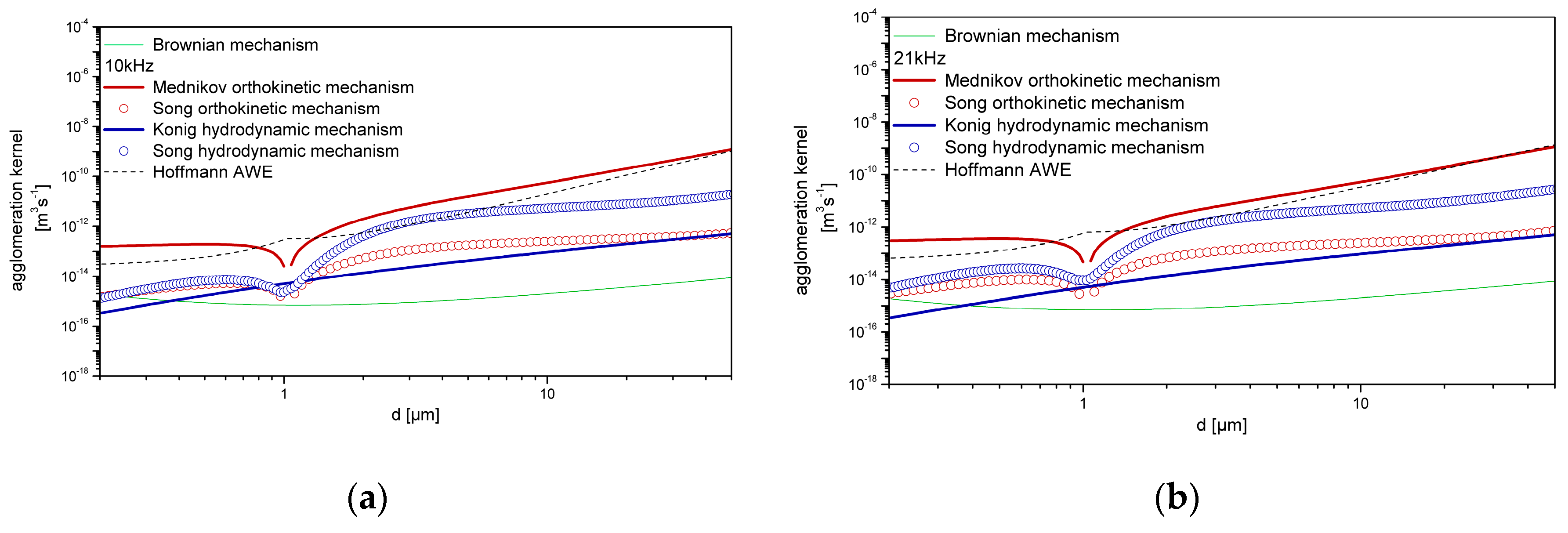
Figure 6.
Temporal evolution of the non-dimensional particle number concentration.
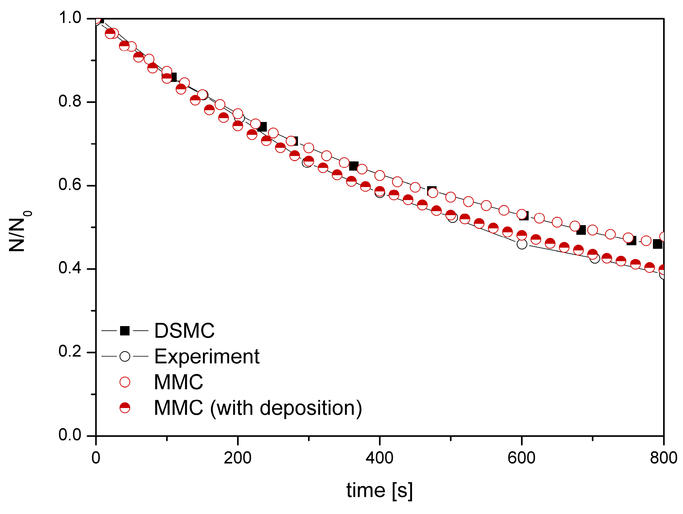
Figure 7.
Temporal evolution of the non-dimensional particle number concentration and comparison with the DSMC and experimental results, for various acoustic kernel combinations and for two acoustic frequencies (a) 10 kHz; (b) 21 kHz.
Figure 7.
Temporal evolution of the non-dimensional particle number concentration and comparison with the DSMC and experimental results, for various acoustic kernel combinations and for two acoustic frequencies (a) 10 kHz; (b) 21 kHz.
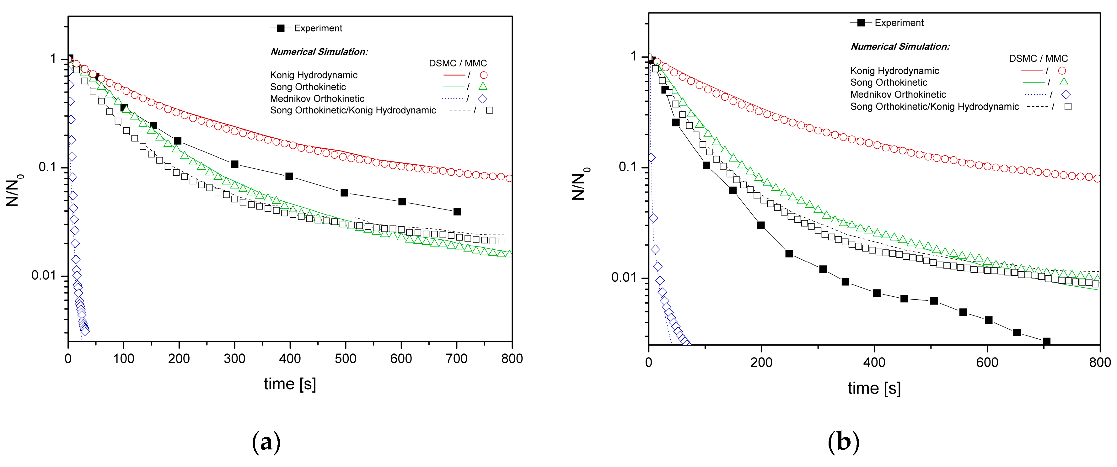
Figure 8.
Temporal evolution of the non-dimensional particle number concentration and comparison with the DSMC and experimental results, for the hydrodynamic mechanism as modified by Song (a) and for the AWE kernel (b).
Figure 8.
Temporal evolution of the non-dimensional particle number concentration and comparison with the DSMC and experimental results, for the hydrodynamic mechanism as modified by Song (a) and for the AWE kernel (b).
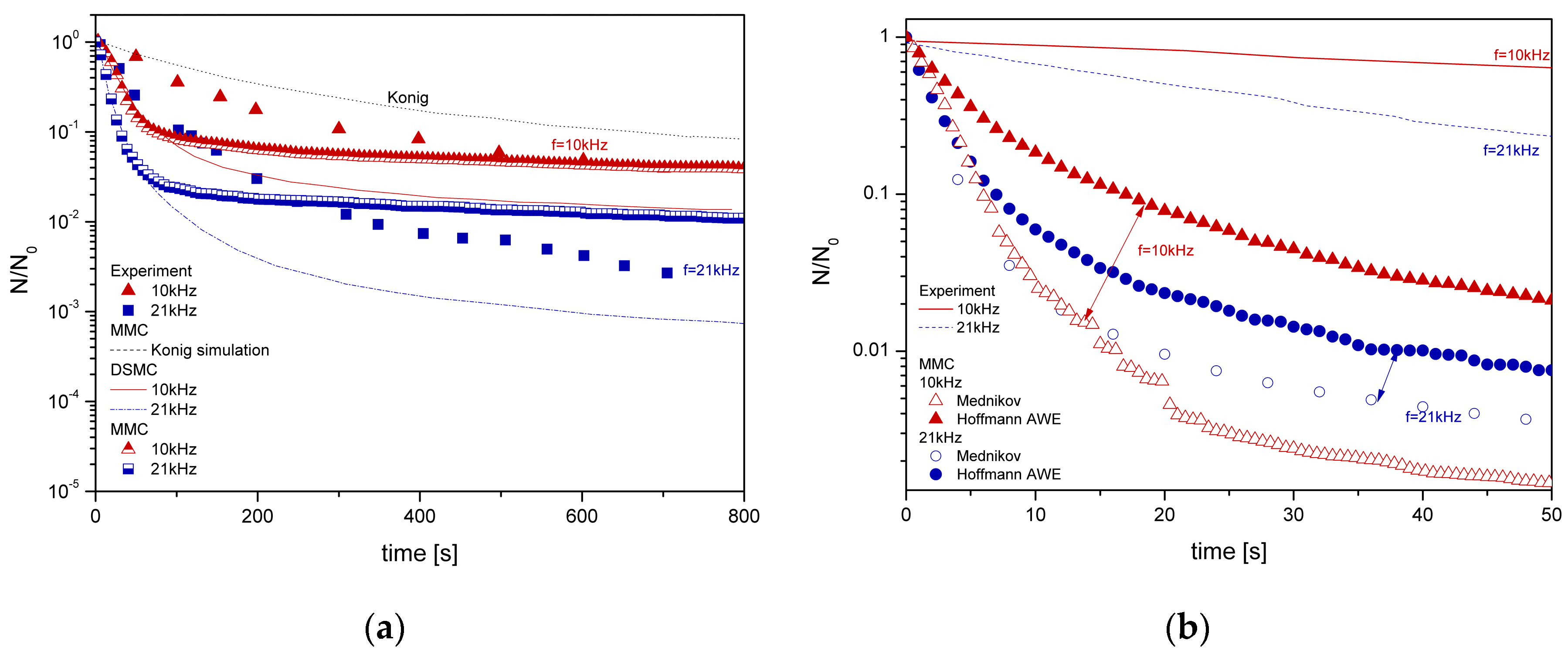
Figure 9.
Snapshots of the particle size distribution evolution: initial distribution and the distribution observed after 400 s of acoustic treatment (100 W, f = 10 kHz). Acoustic agglomeration is simulated utilizing the following kernels: (a) βSong,Or; (b) βSong,Or +βKönig,Hy.
Figure 9.
Snapshots of the particle size distribution evolution: initial distribution and the distribution observed after 400 s of acoustic treatment (100 W, f = 10 kHz). Acoustic agglomeration is simulated utilizing the following kernels: (a) βSong,Or; (b) βSong,Or +βKönig,Hy.
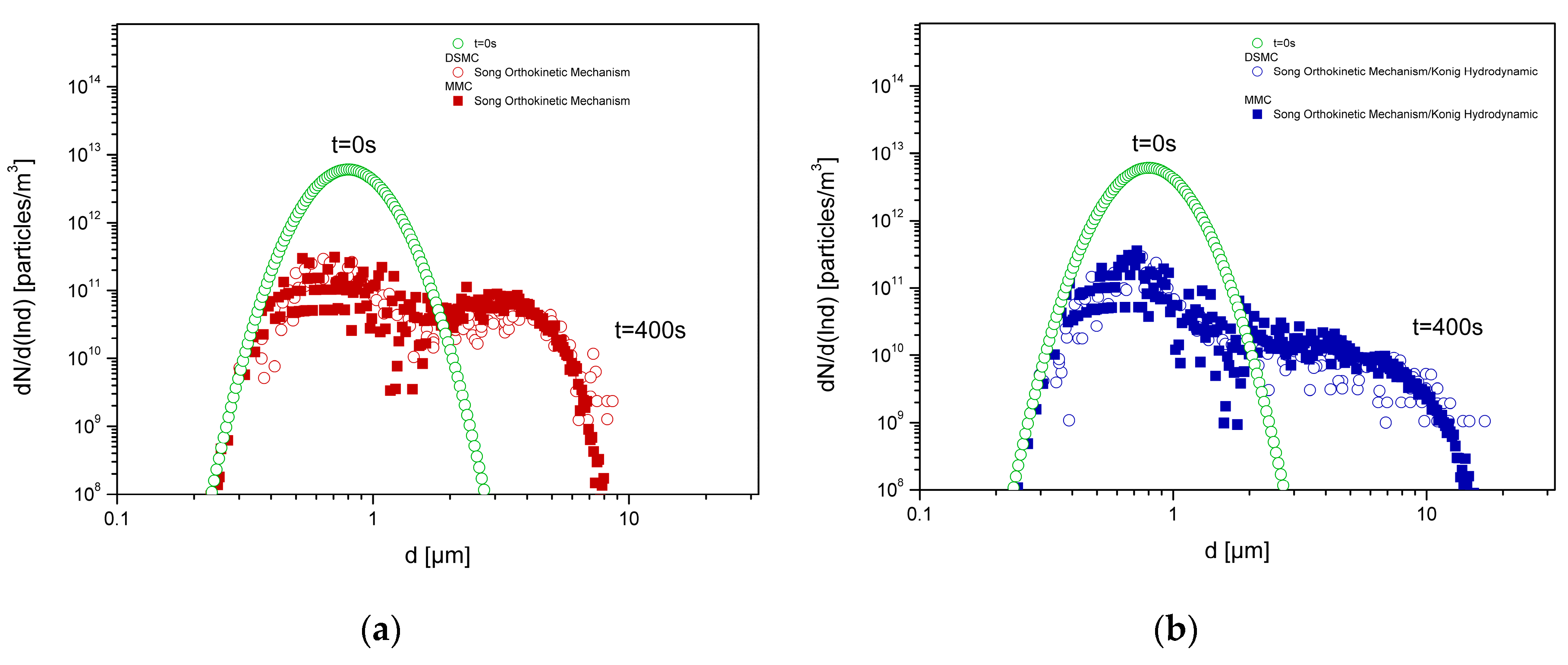
Figure 10.
Temporal evolution of the mean mass diameter (a) and the mean number diameter (b) of the particle size distribution (geometric values) during the simulation of acoustic agglomeration utilizing two distinct kernels (100 W, f = 10 kHz).
Figure 10.
Temporal evolution of the mean mass diameter (a) and the mean number diameter (b) of the particle size distribution (geometric values) during the simulation of acoustic agglomeration utilizing two distinct kernels (100 W, f = 10 kHz).
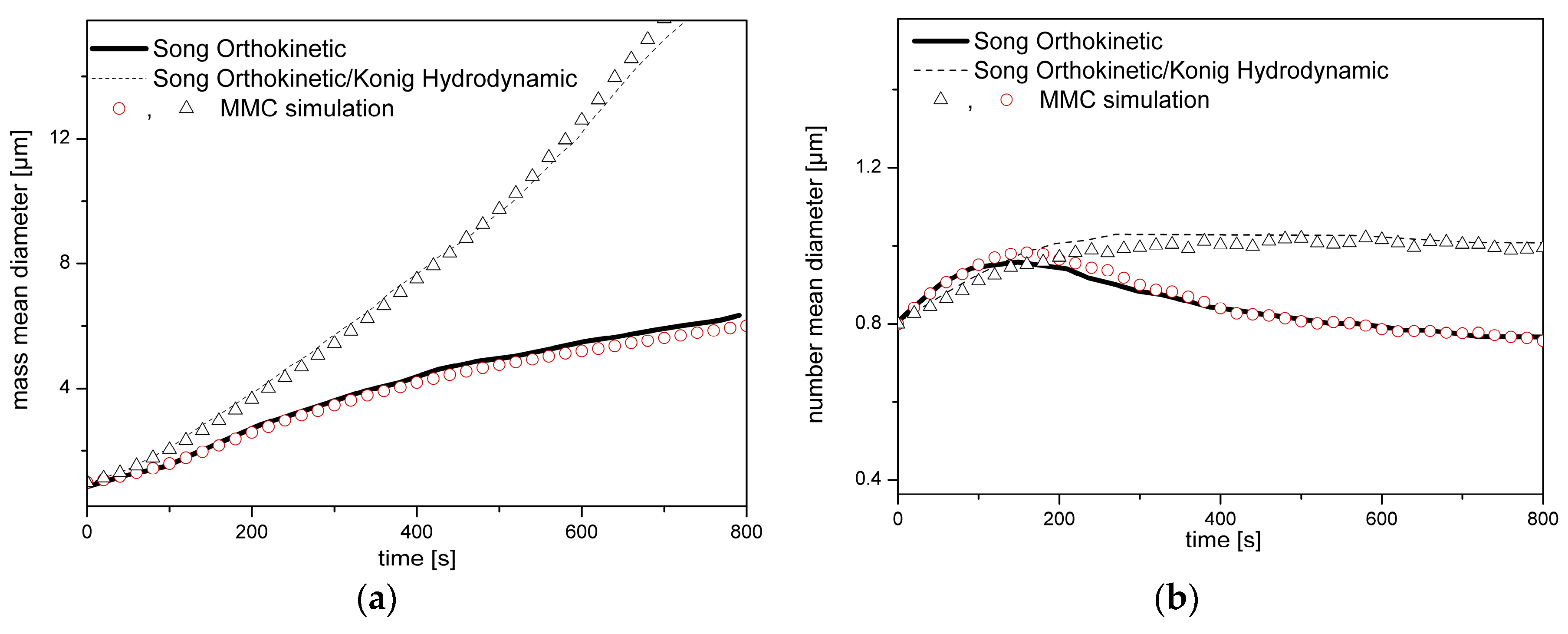
Figure 11.
Temporal evolution of the non-dimensional particle number concentration for various acoustic sound intensities. The sound frequency is (a) 10 kHz and (b) 21 kHz.
Figure 11.
Temporal evolution of the non-dimensional particle number concentration for various acoustic sound intensities. The sound frequency is (a) 10 kHz and (b) 21 kHz.
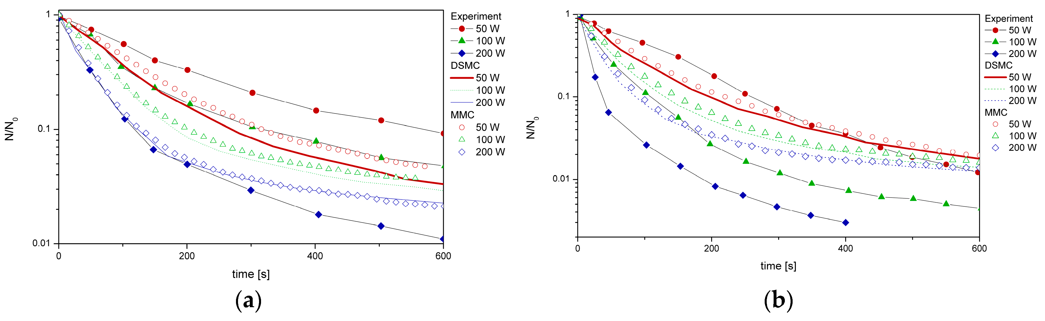
Figure 12.
Temporal evolution of the non-dimensional particle number concentration for various acoustic sound intensities. The experimental results of (a) Caperan and (b) Magill have been used.
Figure 12.
Temporal evolution of the non-dimensional particle number concentration for various acoustic sound intensities. The experimental results of (a) Caperan and (b) Magill have been used.
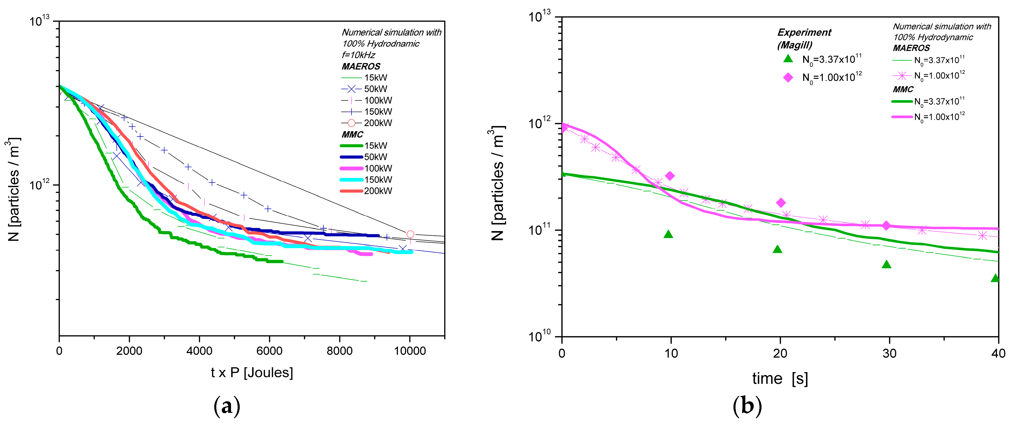
Figure 13.
Temporal evolution of the non-dimensional particle number concentration for various acoustic sound intensities and two distinct sound frequencies. Acoustic agglomeration is simulated utilizing the acoustic wake kernel.
Figure 13.
Temporal evolution of the non-dimensional particle number concentration for various acoustic sound intensities and two distinct sound frequencies. Acoustic agglomeration is simulated utilizing the acoustic wake kernel.
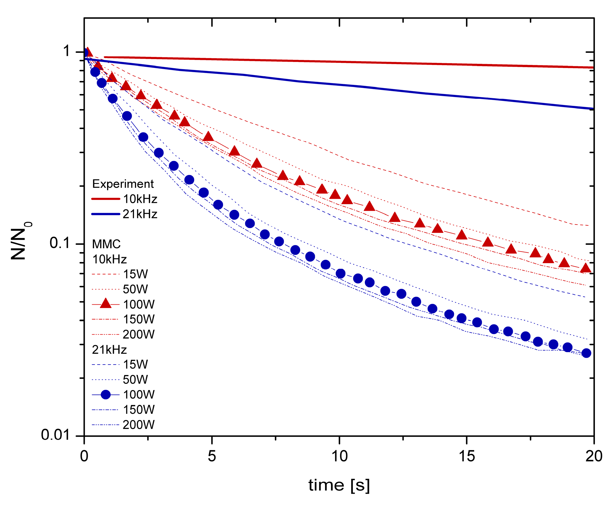
Figure 14.
Temporal evolution of the particle number concentration for various initial particle number concentrations. Acoustic agglomeration is simulated utilizing the following kernels (a) βSong,Or +βKönig,Hy ; (b) βSong,Or +βSong,Hy.
Figure 14.
Temporal evolution of the particle number concentration for various initial particle number concentrations. Acoustic agglomeration is simulated utilizing the following kernels (a) βSong,Or +βKönig,Hy ; (b) βSong,Or +βSong,Hy.
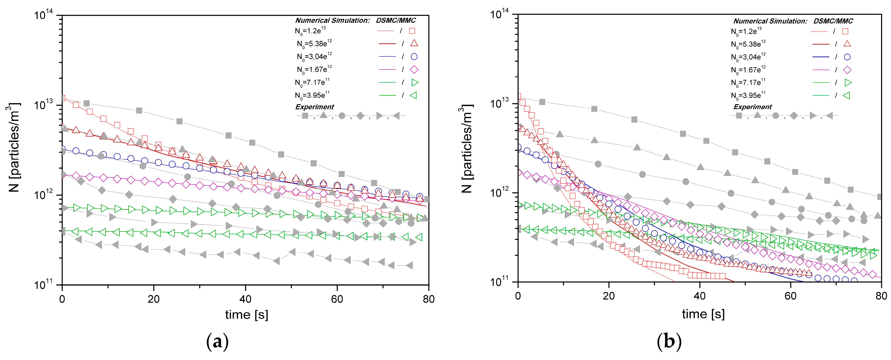
Figure 15.
Curves showing the variation of the particle entrainment factor vs the particle size diameter. The particle cumulative size distribution curves, for three different initial shapes, are also shown.
Figure 15.
Curves showing the variation of the particle entrainment factor vs the particle size diameter. The particle cumulative size distribution curves, for three different initial shapes, are also shown.
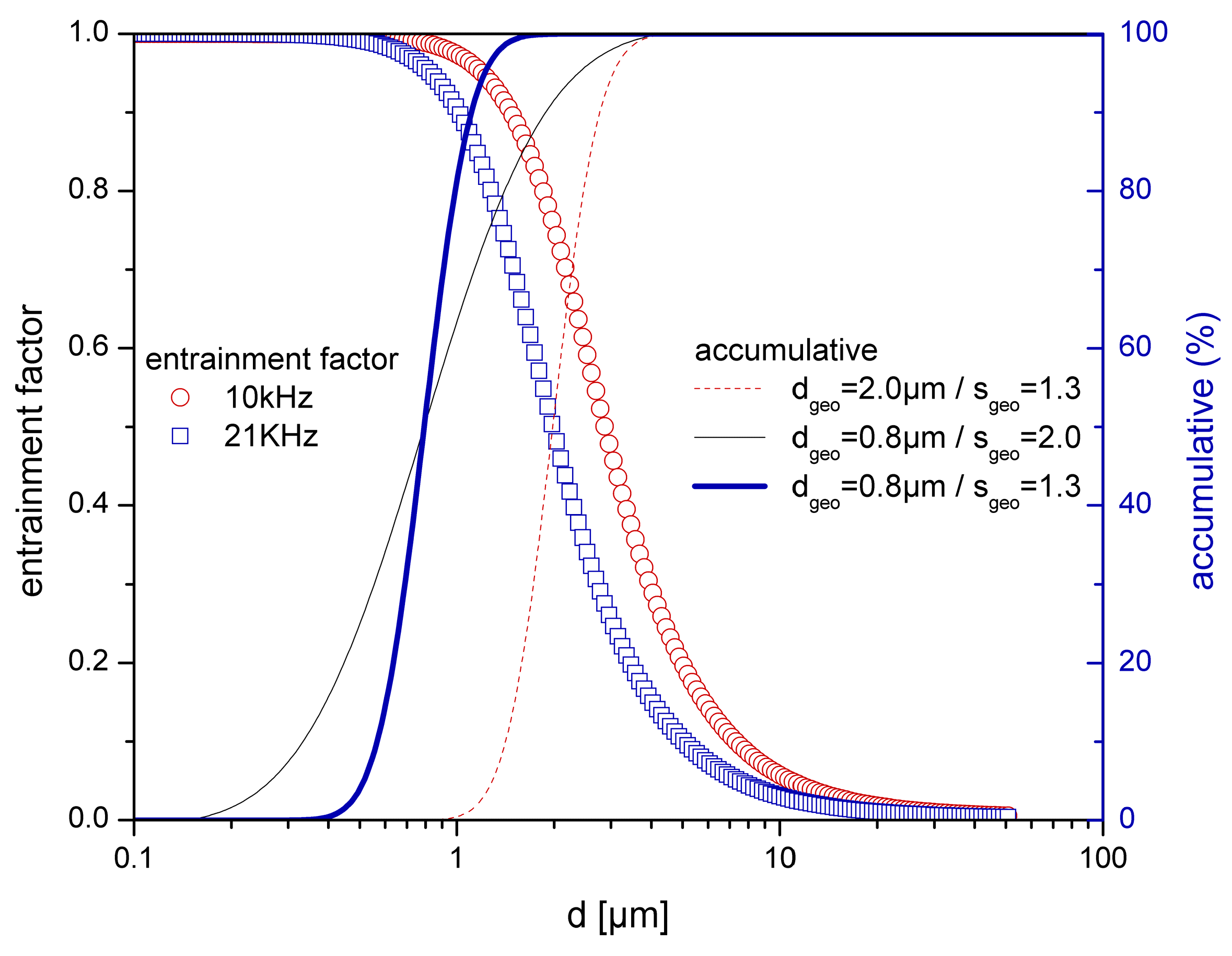
Figure 16.
(a) Temporal evolution of the non-dimensional particle number concentration for varied initial particle size distributions. (b) Snapshots of the particle distribution after 50 s of acoustic treatment are displayed (f = 10 kHz, 100 W).
Figure 16.
(a) Temporal evolution of the non-dimensional particle number concentration for varied initial particle size distributions. (b) Snapshots of the particle distribution after 50 s of acoustic treatment are displayed (f = 10 kHz, 100 W).
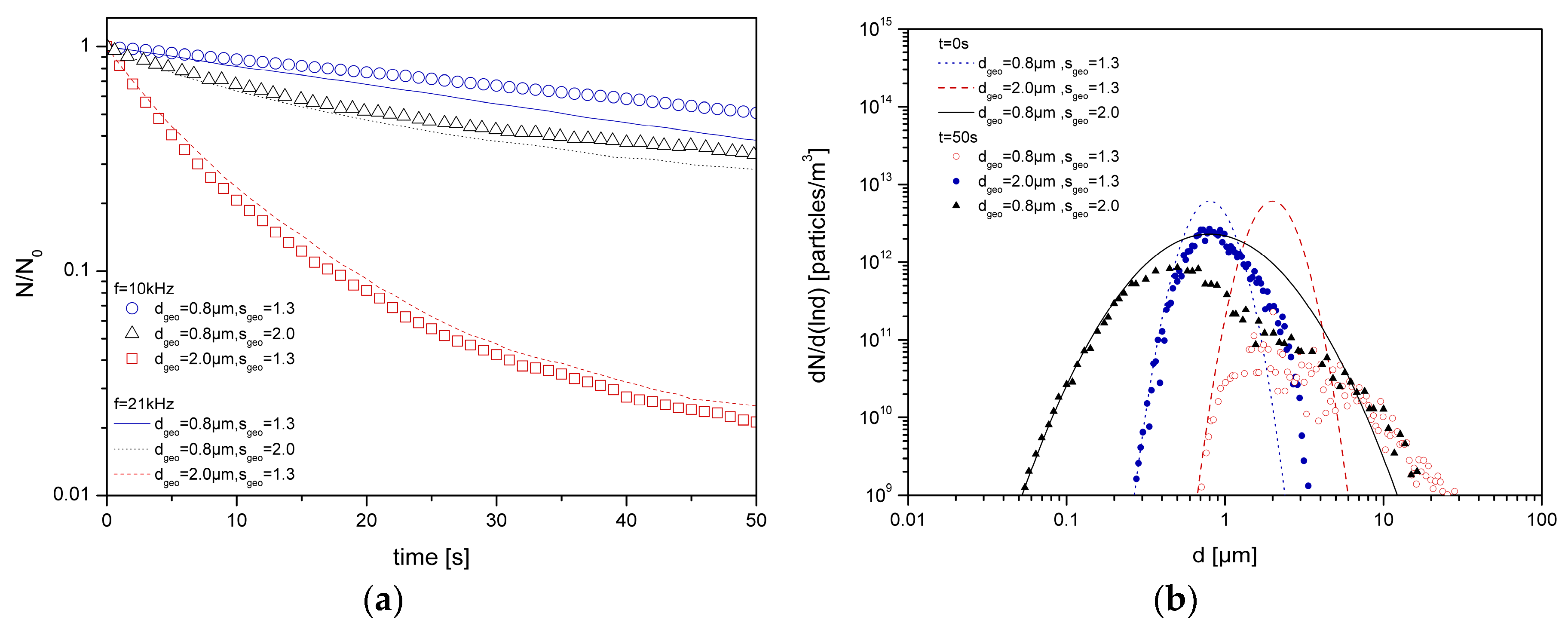
Figure 17.
(a) Particle entrainment factor, for two distinct particle densities and frequencies of the acoustic field. (b) Temporal evolution of the non-dimensional particle number concentration. Acoustic agglomeration is simulated utilizing the following kernel: βSong,Or +βKönig,Hy.
Figure 17.
(a) Particle entrainment factor, for two distinct particle densities and frequencies of the acoustic field. (b) Temporal evolution of the non-dimensional particle number concentration. Acoustic agglomeration is simulated utilizing the following kernel: βSong,Or +βKönig,Hy.
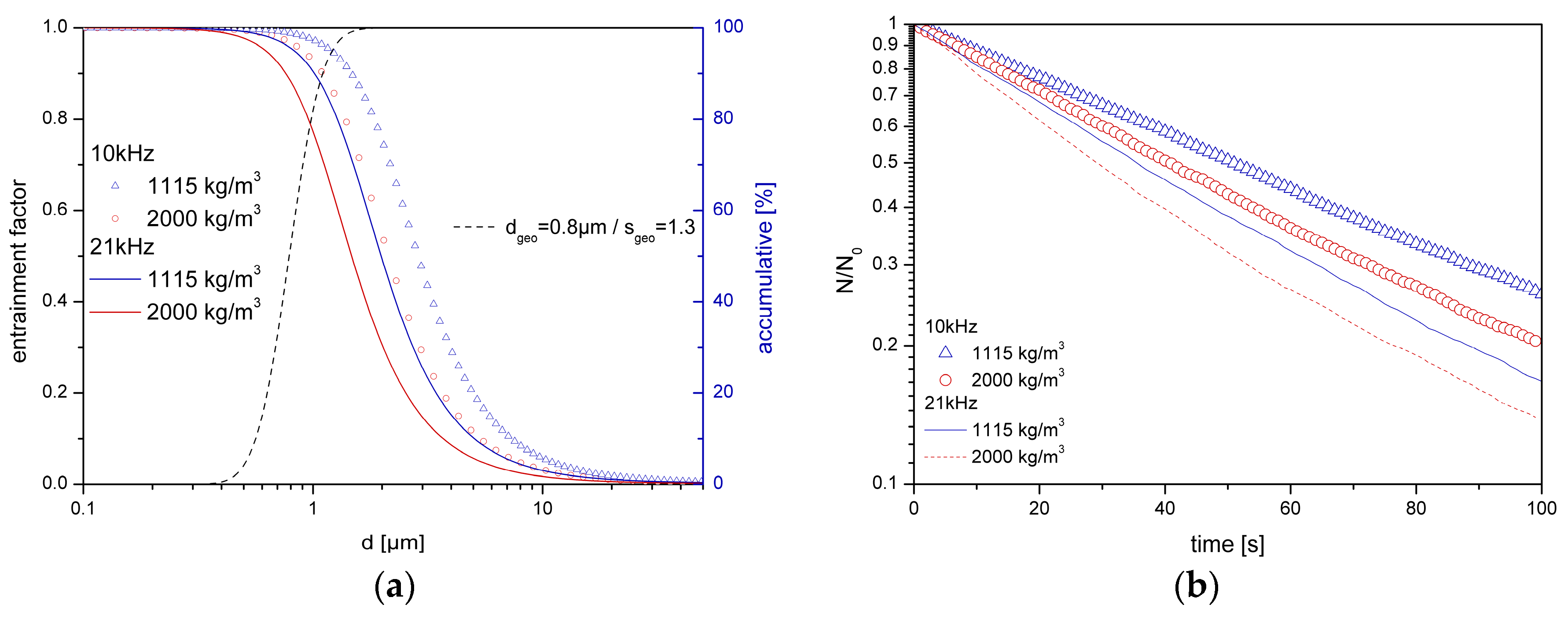
Figure 18.
Snapshots of the particle size distribution evolution after 100 s of acoustic treatment, for (a) 10 kHz; (b) 21 kHz. Acoustic agglomeration is simulated utilizing the following kernel: βSong,Or +βKönig,Hy.
Figure 18.
Snapshots of the particle size distribution evolution after 100 s of acoustic treatment, for (a) 10 kHz; (b) 21 kHz. Acoustic agglomeration is simulated utilizing the following kernel: βSong,Or +βKönig,Hy.
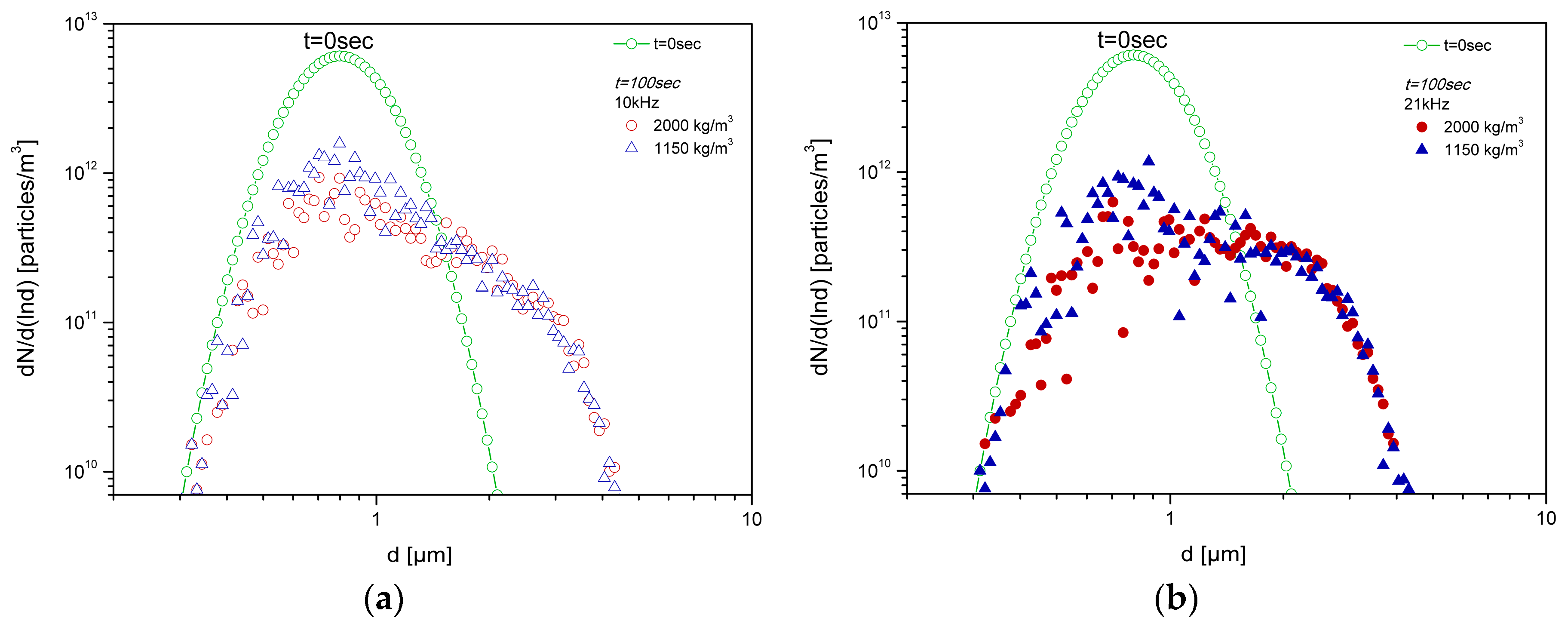
Figure 19.
(a) Particle entrainment factor, for various frequencies of the acoustic field along with cumulative particle size distribution. (b) The calculated hydrodynamic interaction factor g12 is plotted for one particle of 0.8 μm and a particle with a diameter ranging from 0.1 μm to 10 μm.
Figure 19.
(a) Particle entrainment factor, for various frequencies of the acoustic field along with cumulative particle size distribution. (b) The calculated hydrodynamic interaction factor g12 is plotted for one particle of 0.8 μm and a particle with a diameter ranging from 0.1 μm to 10 μm.
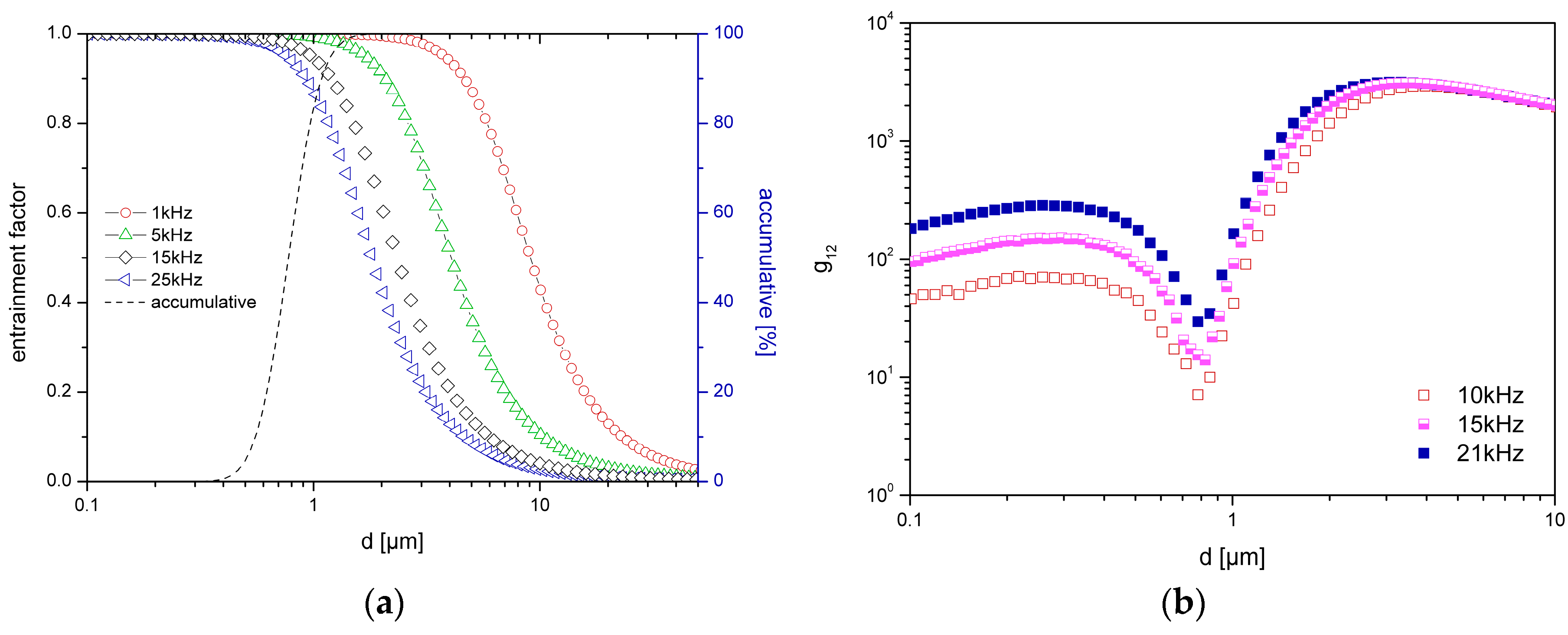
Figure 20.
The effect of the sound frequency (10 kHz and 21 kHz) on the acoustic agglomeration kernel, proposed by Mednikov and Hoffmann (AWE). The intensity of the sound field is the same (100 W) and the results are for one particle of 1 μm and a second particle with diameter ranging from 0.1 μm to 10 μm.
Figure 20.
The effect of the sound frequency (10 kHz and 21 kHz) on the acoustic agglomeration kernel, proposed by Mednikov and Hoffmann (AWE). The intensity of the sound field is the same (100 W) and the results are for one particle of 1 μm and a second particle with diameter ranging from 0.1 μm to 10 μm.
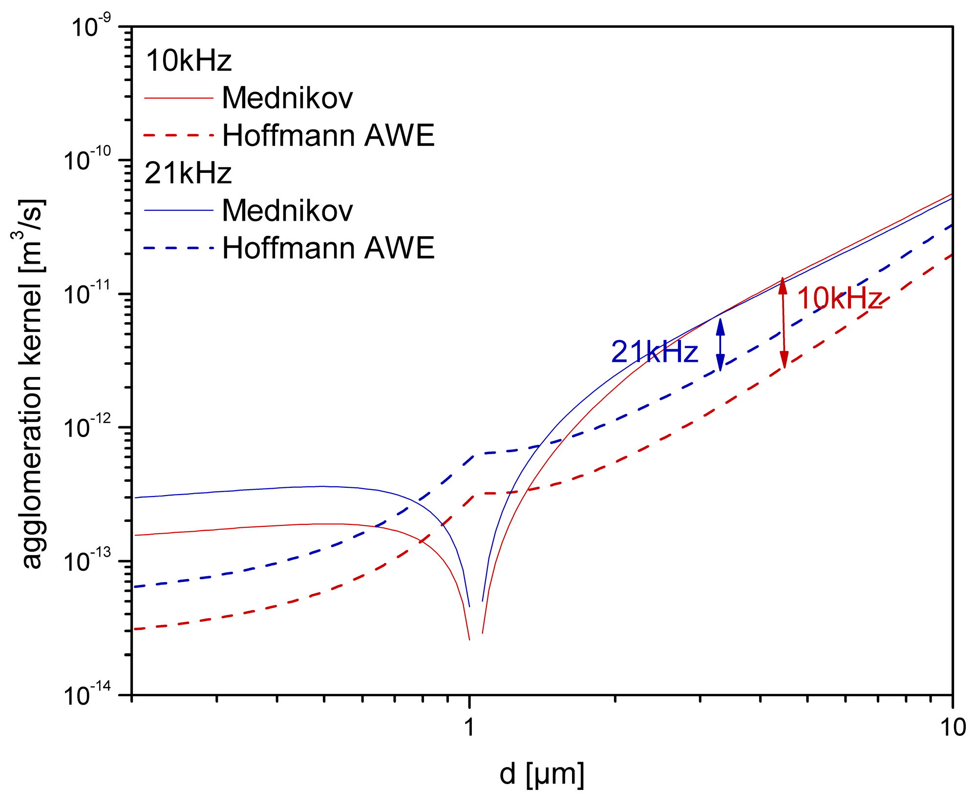
Figure 21.
(a) Temporal evolution of the non-dimensional particle number concentration for various sound frequencies with fixed sound intensity of 100 W; (b) Particle size distributions at 100 s of acoustic treatment (compared with the initial) for various frequencies.
Figure 21.
(a) Temporal evolution of the non-dimensional particle number concentration for various sound frequencies with fixed sound intensity of 100 W; (b) Particle size distributions at 100 s of acoustic treatment (compared with the initial) for various frequencies.
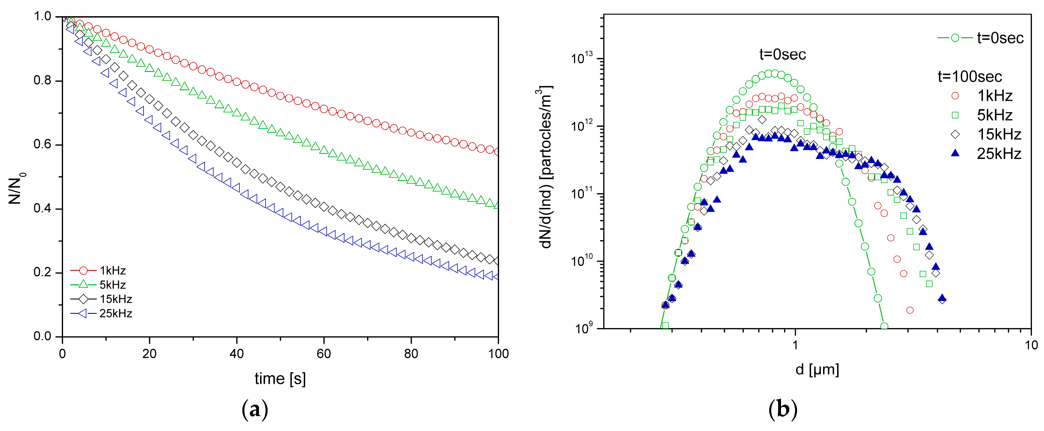

Table 1.
Parameters of the two experimental setups utilized as reference in the numerical simulation of acoustic agglomeration.
Table 1.
Parameters of the two experimental setups utilized as reference in the numerical simulation of acoustic agglomeration.
| Parameter | Caperan | Magill |
| Initial particle number concentration, [particles/m3] | 4 × 10¹² | 3.3 × 10¹¹–5.5 × 10¹² |
| Initial geometric standard deviation | 1.30 | 1.35 |
| Initial geometric mean particle diameter, [μm] | 0.8 | 0.8 |
| Temperature, [°C] | 20 | 20 |
| Fluid dynamic viscosity, [Pa·s] | 1.8 × 10⁻⁵ | 1.8 × 10⁻⁵ |
| Fluid density, [kg/m3] | 1.2 | 1.2 |
| Particle density, [kg/m3] | 1115 | 1115 |
| Sound Intensity | 100 W–200 W | 155 dB |
| Sound Frequency, [kHz] | 10-21 | 9.4 |
Disclaimer/Publisher’s Note: The statements, opinions and data contained in all publications are solely those of the individual author(s) and contributor(s) and not of MDPI and/or the editor(s). MDPI and/or the editor(s) disclaim responsibility for any injury to people or property resulting from any ideas, methods, instructions or products referred to in the content. |
© 2026 by the authors. Licensee MDPI, Basel, Switzerland. This article is an open access article distributed under the terms and conditions of the Creative Commons Attribution (CC BY) license (http://creativecommons.org/licenses/by/4.0/).
Copyright: This open access article is published under a Creative Commons CC BY 4.0 license, which permit the free download, distribution, and reuse, provided that the author and preprint are cited in any reuse.


