Submitted:
28 April 2026
Posted:
30 April 2026
You are already at the latest version
Abstract
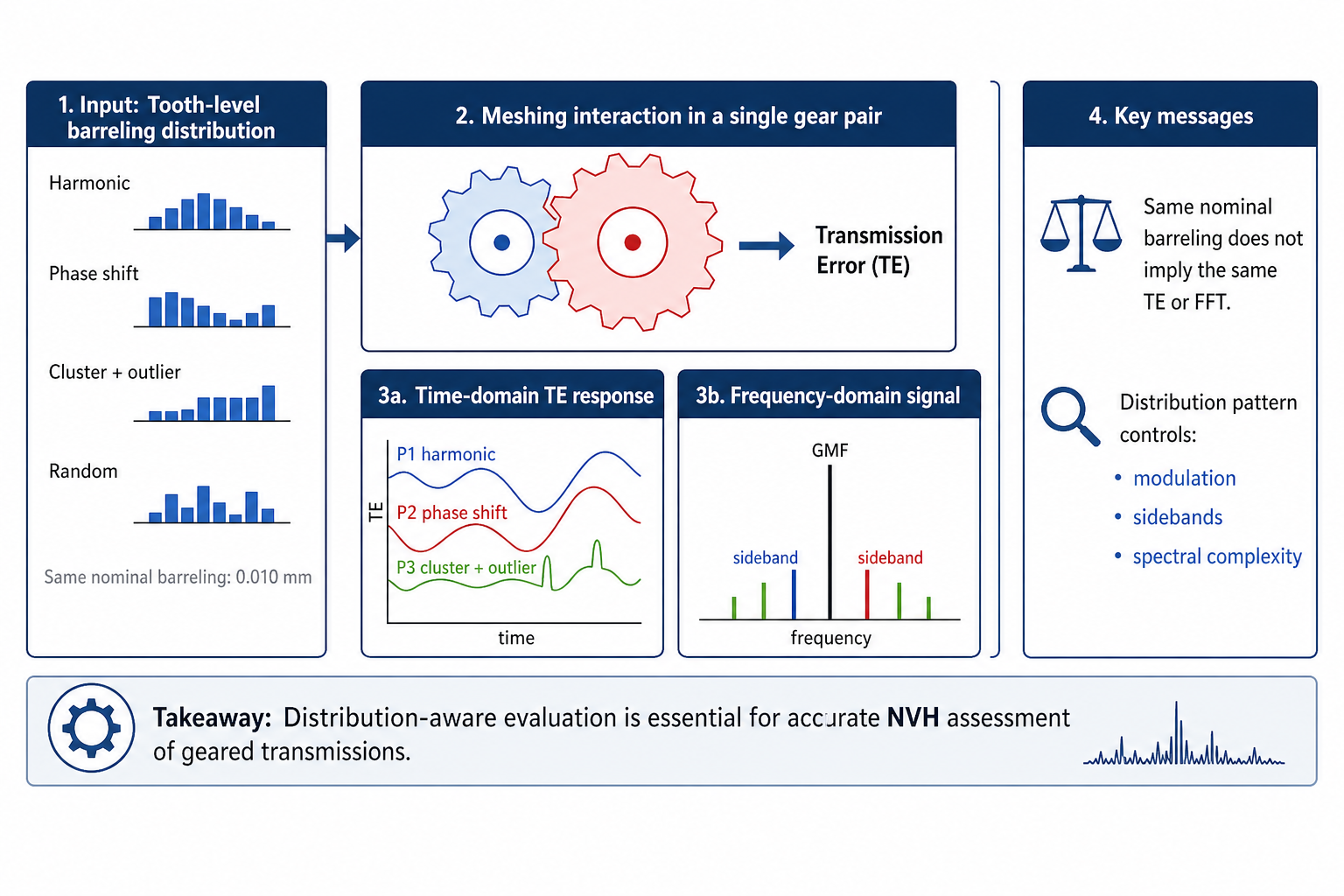
Transmission error (TE) is widely recognized as the primary internal excitation source in geared systems and plays a central role in vibration and noise generation. While micro-geometry modifications such as barreling are typically defined through nominal parame-ter values, the spatial distribution of tooth-level deviations is often neglected in simula-tion-based NVH assessments. In this study, the influence of tooth-by-tooth barreling dis-tribution on TE and its frequency-domain response was investigated using a controlled single gear-pair simulation model. A constant nominal barreling value was maintained across all cases, while only the spatial distribution of deviations was varied. Four repre-sentative patterns were considered: harmonic, phase-shifted harmonic, clustered with an outlier, and random.The results show that different distribution patterns lead to clearly distinguishable TE signals and FFT spectra, despite identical nominal modification levels. Harmonic distributions produce regular, periodic responses with clean spectral signa-tures. In contrast, phase-shifted patterns introduce modulation effects and sideband structures around the gear mesh frequency (GMF). Clustered deviations generate localized peaks and fault-like spectral features, while random distributions result in broader, less structured excitation. These findings indicate that the NVH-relevant effect of microgeome-try cannot be described solely by nominal amplitude. The spatial distribution of tooth-level deviations significantly influences both the temporal structure and spectral content of TE. The study highlights the importance of incorporating distribution-aware approaches in simulation-driven gear NVH analysis.
Keywords:
gear dynamics
; transmission error
; barreling
; microgeometry
; tooth-to-tooth variability
; gear mesh frequency
; sidebands
; modulation
; NVH
; multibody simulation
1. Introduction
The acoustic behavior of modern drivetrain systems is increasingly governed by internal excitation mechanisms rather than external noise sources. In this context, transmission error (TE) is widely recognized as the primary excitation source in geared systems, as it directly reflects deviations from ideal kinematic motion and governs the dynamic mesh forces responsible for vibration and noise generation [1,2].
In classical gear dynamics theory, TE is defined as the deviation between the actual and ideal angular position of the driven gear. Both static and dynamic components of TE have been extensively investigated, and their relationship to mesh stiffness variation, contact conditions, and structural dynamics has been well established [2,3,4]. In particular, time-varying mesh stiffness and contact nonlinearity are known to introduce periodic excitation components that are directly linked to the gear mesh frequency (GMF) and its harmonics [3,4].
Microgeometry modifications, such as profile relief and lead crowning (barreling), are commonly applied in order to control load distribution and reduce excitation levels [5]. These modifications are typically defined through nominal parameters and are assumed to be uniformly applied across all teeth. In practice, however, this assumption is rarely fully satisfied. Manufacturing processes introduce tooth-to-tooth variability due to tool wear, alignment deviations, and process scatter, leading to non-uniform microgeometry along the gear circumference [6,7].
Previous studies have shown that manufacturing deviations can significantly influence TE and vibration levels, particularly in applications where tonal components are not masked by stronger background sources [7,8]. However, most simulation-based approaches focus primarily on the magnitude of deviations, while the spatial distribution of these deviations is often treated implicitly or neglected. As a result, the potential role of tooth-level distribution as an excitation-shaping factor remains insufficiently explored.
From a signal analysis perspective, the structure of TE is directly reflected in its frequency-domain representation. Periodic excitation leads to dominant peaks at the GMF, while modulation effects introduce sidebands spaced by shaft rotational frequency [3,9]. Such sideband structures are commonly associated with faults or localized defects, but similar spectral features may also arise from structured or non-uniform microgeometry distributions. This raises an important question: to what extent can different spatial patterns of nominally identical deviations produce distinguishable spectral signatures?
Recent advances in simulation tools have enabled the definition of individual tooth-level microgeometry, allowing deviations to be assigned independently to each tooth [10]. This provides an opportunity to investigate not only the amplitude, but also the spatial structure of microgeometry variability in a controlled manner. Despite this capability, systematic studies focusing specifically on distribution-driven effects remain limited.
The present study addresses this gap by investigating the influence of tooth-level barreling distribution on transmission error and its spectral characteristics using a controlled single gear-pair model. A constant nominal barreling value is maintained in all simulations, while only the spatial distribution of deviations is varied. Four representative patterns are considered: harmonic, phase-shifted harmonic, clustered with an outlier, and random.
The objective is not to provide a full-system NVH prediction, but to isolate and interpret the underlying excitation mechanisms associated with different distribution types. By comparing time-domain TE signals and their FFT representations, the study aims to clarify how spatial microgeometry variability influences modulation behavior, sideband formation, and overall spectral complexity.
2. Materials and Methods
2.1. Simulation Framework
The present investigation was carried out in a controlled multibody simulation environment representing a single cylindrical gear pair. The purpose of the model was not to reproduce a complete industrial drivetrain, but to isolate the influence of tooth-level barreling distribution on transmission error and its spectral characteristics under clearly defined boundary conditions.
The simulation workflow was based on the individual-tooth microgeometry concept described in the Adams Gear AT tutorial, where deviations are applied relative to a nominal microgeometry definition on a tooth-by-tooth basis. In the original tutorial, the same framework is demonstrated for tip relief distribution and subsequent TE/FFT evaluation. The present study adopted the same general approach but applied it to barreling-related deviations in a structured 16-run sensitivity matrix.
The overall simulation and evaluation workflow is summarized in Figure 1. First, the baseline gear-pair model was evaluated using the nominal microgeometry definition. Then, tooth-level barreling deviation patterns were introduced according to the 16-run test matrix. For each simulation, the TE time signal was extracted and transformed into the frequency domain using FFT. Finally, the results were compared by distribution group in order to identify changes in waveform structure, GMF response, sideband behavior, and spectral complexity.
2.2. Gear Model and Operating Condition
The investigated model represents a single-stage cylindrical helical gear pair. The basic geometry is summarized in Table 1. The pinion contains 23 teeth and the wheel contains 81 teeth. Both gears have a normal module of 1.395 mm and a normal pressure angle of 20°. Opposite helix angles of −24° and +24° were applied to the pinion and wheel, respectively. The face widths were 30 mm for the pinion and 28 mm for the wheel. The pinion was operated at a constant speed of 200 rpm.
Based on the 23-tooth pinion and the imposed rotational speed, the shaft rotational frequency and the theoretical gear mesh frequency are:
The resulting gear ratio is:
Thus, the dominant mesh-related spectral component is expected near 76.67 Hz, while sideband components are expected to be spaced by approximately 3.33 Hz around the gear mesh frequency.
2.3. Baseline Microgeometry Definition
The baseline microgeometry settings were kept constant in all simulations. The following common settings were applied:
- modified gear: pinion only
- modified flank: Profile Right
- distribution mode: Individual per Tooth
- nominal tip relief amount: 0.020 mm
- tip relief start position: 70%
- relief length: default
- wheel microgeometry: not modified
These settings are consistent with the project definition used for the simulation study, in which the nominal tip relief remained fixed and only the tooth-level deviation pattern was varied.
For the barreling study, the nominal lead-direction modification was defined as:
- nominal barreling value: 0.010 mm
- barreling shape: Quadratic
This nominal barreling value remained unchanged in all runs. Consequently, the simulations did not compare different baseline barreling designs, but instead examined how different tooth-level deviation distributions around the same nominal value affected the response.
The actual barreling value of a given tooth was defined as
where is the actual barreling of tooth i, is the nominal barreling value, and Δ is the tooth-level deviation.
Thus, the spatial pattern of Δ was the only microgeometry-related quantity that changed between runs.
2.4. Distribution Patterns
To represent different forms of tooth-level variability, four distribution patterns were defined.
2.4.1. Harmonic Distribution (P1)
In the first pattern, the barreling deviation was distributed harmonically along the tooth sequence. This created a smooth, periodic tooth-to-tooth variation. The purpose of this case was to represent a structured and deterministic circumferential deviation pattern.
2.4.2. Phase-Shifted Harmonic Distribution (P2)
The second pattern used the same harmonic deviation magnitude as P1 but with a phase shift. This preserved the nominal amplitude level while altering the spatial alignment of the deviation pattern relative to the tooth sequence. The case was introduced to examine how phase relocation of an otherwise similar pattern affects the TE waveform and sideband behavior.
2.4.3. Cluster + Outlier Distribution (P3)
The third pattern represented a localized tooth-level deviation scenario. A cluster of neighboring teeth was assigned elevated deviation values, and one additional tooth was assigned an even larger value, referred to as an outlier. In the investigated 23-tooth configuration, the cluster was assigned to teeth 6–9, while tooth 17 served as the outlier. All remaining teeth retained zero deviation.
This pattern was designed to represent a simplified localized irregularity, such as concentrated manufacturing deviation, local wear accumulation, or a single strongly deviating tooth.
2.4.4. Random Distribution (P4)
In the fourth pattern, zero-mean deviation values were assigned randomly across the tooth set within a prescribed amplitude range. This case was used to represent tooth-to-tooth variability without deterministic spatial structure, analogous to manufacturing scatter.
2.5. Test Matrix
A total of 16 simulation runs were performed. Four amplitude levels were combined with the four distribution patterns:
- S1: ±0.002 mm
- S2: ±0.004 mm
- S3: ±0.006 mm
- S4: ±0.008 mm
The simulation matrix was organized as follows:
- Runs 1–4: P1 harmonic distribution
- Runs 5–8: P2 phase-shifted harmonic distribution
- Runs 9–12: P3 cluster + outlier distribution
- Runs 13–16: P4 random distribution
For the harmonic and phase-shifted harmonic cases, the deviation distribution was generated using the harmonic distribution function within the microgeometry definition workflow. For the cluster + outlier and random cases, tooth-level values were defined explicitly through the deviation table, consistent with the project setup.
2.6. Solver and Simulation Settings
The same numerical and post-processing settings were used for all 16 simulations in order to ensure direct comparability between the investigated deviation patterns. The most relevant solver and FFT settings are summarized in Table 2.
The initial startup transient was excluded from the frequency-domain interpretation. Therefore, the FFT analysis was performed on the stabilized portion of the TE signal using the 0.15–0.7 s time window. This ensured that the spectral comparison focused on steady-state gear meshing behavior rather than transient startup effects.
The theoretical shaft rotational frequency was 3.33 Hz, and the theoretical gear mesh frequency was 76.67 Hz. Therefore, sideband components around the GMF were interpreted using the shaft rotational frequency as the expected modulation spacing.
2.7. Transmission Error Evaluation
The primary output of the study was the transmission error (TE) time signal. Transmission error was defined as the deviation between the actual and ideal motion of the driven gear, expressed as an equivalent displacement along the line of action.
The TE signal was extracted from the kinematic response of the gear pair and evaluated over the simulated time history. The analysis focused on the steady-state portion of the response, ensuring that the evaluated signal reflects stabilized gear meshing conditions.
The time-domain evaluation was performed using qualitative criteria to capture structural differences between the investigated distribution patterns. The following aspects were considered:
- regularity and periodicity of the waveform
- waveform asymmetry
- amplitude evolution with increasing deviation level
- presence of localized peaks
- degree of signal smoothness or irregularity
This qualitative assessment allowed the identification of distribution-dependent changes in the temporal structure of the excitation, independent of purely amplitude-based effects.
2.8. Frequency-Domain Analysis
The frequency-domain behavior of TE was evaluated using Fast Fourier Transform (FFT). Following the tutorial workflow, the FFT was performed on the TE signal over a selected time window after the initial transient, with detrending enabled. In the tutorial example, an FFT evaluation interval of 0.15–0.7 s is used to compare constant and individual microgeometry cases. The same principle was applied here: only the stabilized part of the TE signal was considered for spectral interpretation.
The FFT analysis focused on:
- identification of the dominant GMF
- observation of sidebands around the GMF
- low-frequency peaks associated with shaft rotation
- comparison of spectral structure between distribution patterns
Particular attention was given to sideband interpretation. Since the shaft rotational frequency is approximately 3.33 Hz, sidebands around the GMF were interpreted in relation to this spacing. Low-frequency peaks below 20 Hz were also examined, as they correspond to the shaft frequency and its harmonics, and therefore provide physical context for modulation-related features.
2.9. Comparative Evaluation Strategy
The study was designed as a comparative sensitivity analysis rather than an absolute NVH prediction model. For this reason, the results were interpreted in relative terms across the 16 runs.
The evaluation addressed the following questions:
- Does the TE waveform remain smooth and periodic, or does it become asymmetric, localized, or irregular?
- Does the FFT remain concentrated around the GMF, or does additional modulation-related content appear?
- Which distribution patterns generate the most structured, the most modulated, or the most fault-like excitation signatures?
- Can different spatial patterns with identical nominal barreling lead to qualitatively different TE and FFT responses?
This framework made it possible to distinguish amplitude effects from distribution effects and to assess whether the tooth-level distribution itself acts as an excitation-shaping factor.
3. Results
The results are presented in two domains: time-domain transmission error behavior and frequency-domain spectral characteristics.
3.1. Time-Domain Transmission Error Response
The transmission error signals exhibited clear and systematic differences between the investigated tooth-level barreling distribution patterns, although the nominal barreling value remained identical in all simulation runs. This confirms that the response is not governed solely by the baseline microgeometry magnitude, but is also influenced by the spatial arrangement of the applied deviations.
For the harmonic distribution (Runs 1–4), the TE signals remained regular and nearly periodic over the analyzed time interval. Increasing deviation amplitude led to a gradual increase in response magnitude, while the overall waveform shape remained largely stable. This behavior indicates a structured excitation mechanism with limited distortion of the signal form. The corresponding signals are shown in Figure 2.
The phase-shifted harmonic distribution (Runs 5–8) produced a noticeably different time-domain response. The TE waveform became more asymmetric, and the upper and lower portions of the signal no longer evolved in the same way. In particular, the waveform peaks appeared more sensitive to the imposed deviation pattern than the valleys. This indicates that the phase shift altered the temporal structure of the contact response rather than simply scaling the excitation amplitude. The corresponding signals are shown in Figure 3.
The cluster + outlier distribution (Runs 9–12) generated the most distinctive time-domain behavior. Localized peaks and sharper irregularities appeared in the TE signal, particularly at higher deviation levels. These features suggest that specific teeth dominate the excitation process, leading to a response that differs fundamentally from the smoother harmonic cases. The corresponding signals are shown in Figure 4.
The random distribution (Runs 13–16) resulted in a less structured TE response. The waveform appeared more irregular and less clearly periodic, indicating that the excitation energy was distributed across many small tooth-level contributions rather than concentrated in a single deterministic pattern. The corresponding signals are shown in Figure 5.
Overall, the time-domain results demonstrate that identical nominal barreling values can produce fundamentally different excitation behaviors depending on the spatial distribution of tooth-level deviations.

Table 3.
Time-domain interpretation of the TE response for the investigated run groups.
| Run group | Pattern | TE time-signal characteristics | Physical interpretation | Main conclusion |
|---|---|---|---|---|
| Runs 1–4 | Harmonic | The TE waveform is regular and nearly periodic. The amplitude increases with deviation level, while the waveform shape remains similar. | The tooth-level deviation is distributed smoothly and periodically, resulting in a structured excitation mechanism. | Harmonic tooth-level deviations primarily scale TE amplitude while preserving a relatively clean temporal response. |
| Runs 5–8 | Phase-shifted harmonic | The TE waveform becomes more asymmetric. Peaks and valleys do not evolve in the same way, and the waveform shape changes with increasing amplitude. | The phase shift modifies the temporal interaction between consecutive teeth and alters load-sharing behavior. | Phase displacement affects not only response level, but also waveform structure and modulation behavior. |
| Runs 9–12 | Cluster + outlier | Localized peaks and sharper irregularities appear in the TE signal, especially at higher amplitudes. | A small group of affected teeth and one strongly deviating tooth dominate the excitation process. | Localized tooth-level deviations produce the most fault-like time-domain response. |
| Runs 13–16 | Random | The TE response becomes more irregular and less clearly periodic. The signal appears more dispersed and less structured. | The excitation originates from many small uncorrelated deviations distributed across the teeth. | Random tooth-level variability leads to a more scatter-like, variability-driven temporal response. |
3.2. Frequency-Domain Characteristics
The FFT analysis confirmed that the distribution pattern influences not only the time-domain structure of the TE signal, but also its spectral signature.
In all runs, a dominant spectral peak was found near 76.9 Hz, which is in close agreement with the theoretical gear mesh frequency of approximately 76.67 Hz, calculated from the 23-tooth pinion rotating at 200 rpm. This strong agreement indicates that the model and the spectral evaluation are physically consistent. The underlying simulation setup corresponds to the project matrix defined for the single gear-pair study.
The harmonic distribution (Runs 1–4) produced the cleanest spectra. A dominant GMF peak was clearly visible, and the surrounding spectral content remained relatively limited. This suggests a predominantly deterministic excitation pattern with modest modulation.
For the phase-shifted harmonic distribution (Runs 5–8), the FFT spectra became more complex. Additional sideband-like components appeared around the GMF, indicating that the response was no longer purely periodic. These sidebands are consistent with modulation induced by the altered spatial phase of the deviation pattern.
The cluster + outlier distribution (Runs 9–12) yielded the most complex spectral structure. Although the GMF remained identifiable, more pronounced surrounding peaks appeared, resulting in a richer and more irregular sideband structure. Within the present simulation framework, this behavior can be interpreted as a localized, fault-like excitation pattern.
The random distribution (Runs 13–16) resulted in broader spectral spreading. Compared with the harmonic and clustered cases, the energy was less concentrated around the dominant peak and more widely distributed over the frequency range. This behavior is consistent with a variability-driven excitation mechanism.
The low-frequency range below 20 Hz also contained noticeable peaks. These are physically consistent with the shaft rotational frequency and its harmonics. At 200 rpm, the shaft frequency is approximately 3.33 Hz, so peaks near 3.3, 6.7, 10.0, 13.3, and 16.7 Hz are expected. These low-frequency components are especially relevant for the interpretation of modulation effects and sideband spacing around the GMF.
A zoomed FFT view around the GMF is presented in Figure 6, where the relative cleanliness of the harmonic case and the increased sideband activity of the phase-shifted and clustered cases can be observed more clearly.
Table 4.
Frequency-domain interpretation of the FFT response for the investigated run groups.
| Run group | Pattern | FFT characteristics | Physical interpretation | Main conclusion |
|---|---|---|---|---|
| Runs 1–4 | Harmonic | The spectrum is dominated by a strong GMF peak, with relatively limited surrounding spectral content. | The excitation remains predominantly periodic and deterministic. | Harmonic distributions mainly reinforce the GMF response while preserving a relatively clean spectral structure. |
| Runs 5–8 | Phase-shifted harmonic | More visible sidebands appear around the GMF. The spectral content becomes wider and more structured. | The altered phase induces modulation, which manifests as sideband formation. | Phase-shifted distributions modify the excitation mechanism and introduce modulation-related spectral features. |
| Runs 9–12 | Cluster + outlier | The GMF remains dominant, but the surrounding spectral region becomes more complex, with stronger sideband activity and additional components. | Localized deviations produce non-uniform excitation and tooth-dominated response contributions. | Clustered deviations with an outlier generate the most fault-like FFT signature among the investigated cases. |
| Runs 13–16 | Random | The spectral energy is more broadly distributed, and the structure is less concentrated around the GMF. | The excitation is driven by uncorrelated tooth-level variability rather than a single deterministic pattern. | Random distributions produce broader and less structured FFT responses, consistent with manufacturing scatter-like behavior. |
The observed sideband spacing is consistent with the shaft rotational frequency of approximately 3.33 Hz.
3.3. Comparative Interpretation of TE and FFT Responses
The combined time-domain and frequency-domain results show that the investigated patterns should not be interpreted merely as different amplitude cases. Instead, each distribution type generates a distinct response mechanism.
The harmonic case can be regarded as a structured baseline, where the system response remains regular in time and concentrated in frequency. The phase-shifted case demonstrates that a spatial redistribution of the same nominal deviation level is sufficient to introduce asymmetry and modulation. The cluster + outlier case stands out as the most critical pattern, producing both localized temporal features and a complex sideband structure. The random case behaves differently again, with less deterministic structure and more distributed spectral energy.
These differences indicate that the tooth-level distribution of barreling deviations acts as an excitation-shaping factor. In other words, the same nominal barreling value does not necessarily imply the same TE waveform or the same FFT signature.
3.4. Main Findings
Based on the obtained TE and FFT results, the following main findings can be drawn within the investigated simulation framework:
-
The distribution pattern of tooth-level barreling deviations significantly influences the TE response.The results show that the temporal behavior of TE is not determined solely by nominal deviation amplitude, but also by how the deviation is distributed among the teeth.
-
The harmonic distribution provides the most regular response.Among the investigated cases, the harmonic distribution produced the cleanest TE waveform and the simplest FFT structure, with a dominant and clearly identifiable GMF.
-
Phase shift introduces modulation effects.The phase-shifted harmonic pattern altered the waveform asymmetry and generated more visible sidebands around the GMF, indicating modulation linked to spatial distribution rather than only to deviation magnitude.
-
Localized deviations are the most critical.The cluster + outlier case produced the most pronounced localized TE features and the most complex FFT sideband structure, suggesting that concentrated deviations have a disproportionate effect on excitation behavior.
-
Random distributions produce broader, less structured excitation.The random case did not create the strongest deterministic sideband pattern, but instead led to broader spectral spreading, consistent with manufacturing scatter-like behavior.
-
The FFT results are physically consistent with the operating condition.The dominant spectral peak near 76.9 Hz closely matches the expected GMF, while the low-frequency components below 20 Hz are consistent with the shaft rotational frequency and its harmonics.
3.5. Implications of the Findings
At the level of the present article, it is appropriate to formulate the implications of the results as carefully stated partial findings rather than broad universal claims. Based on the investigated single gear-pair simulation framework, the following statements are supported:
-
The results suggest that tooth-level barreling distribution affects not only TE magnitude, but also TE structure.This is evident from the differences between regular, asymmetric, localized, and irregular time-domain responses.
-
Different tooth-by-tooth deviation patterns can produce distinguishable spectral signatures even at the same nominal barreling level.In particular, harmonic, phase-shifted, clustered, and random patterns lead to visibly different GMF-sideband behavior.
-
Localized patterns appear to be more effective in generating fault-like sideband structures than harmonic or random patterns.Within the present simulation setup, the cluster + outlier case produced the most complex and defect-like frequency-domain response.
These statements should be interpreted as simulation-based observations within the investigated framework. Nevertheless, they point to the broader conclusion that distribution-aware microgeometry evaluation may provide additional insight beyond nominal amplitude-based assessments.
4. Discussion
The results demonstrate that tooth-level barreling distribution acts as a key excitation-shaping parameter, influencing not only the amplitude but also the structure of transmission error and its spectral representation.
From a physical perspective, the harmonic distribution represents a smooth spatial variation of microgeometry, leading to a stable load-sharing condition. As a result, the excitation remains predominantly periodic, and the spectral content is concentrated around the GMF. This case can be considered as a baseline representing well-ordered manufacturing variation.
The phase-shifted harmonic distribution highlights that even when the deviation amplitude remains unchanged, the spatial alignment of the pattern relative to the meshing sequence significantly affects the excitation behavior. The observed asymmetry in the TE waveform and the corresponding sidebands in the FFT indicate amplitude modulation. This suggests that phase relationships between consecutive teeth can influence the temporal evolution of contact conditions and, consequently, the spectral signature.
The cluster + outlier distribution introduces a fundamentally different excitation mechanism. The localized concentration of deviations disrupts uniform load sharing and leads to dominant contributions from specific teeth. This results in localized peaks in the TE signal and a more complex spectral structure. Within the limits of the present simulation framework, this behavior shows qualitative similarity to fault-induced excitation patterns, where localized defects generate non-uniform and impulsive responses.
The random distribution further emphasizes the importance of spatial structure. In this case, the absence of a deterministic pattern leads to a more diffuse excitation, where energy is spread across a wider frequency range. This type of response is representative of manufacturing variability, where the lack of correlation between individual deviations prevents the formation of strong deterministic features.
These observations suggest that the commonly used amplitude-based characterization of microgeometry deviations may not be sufficient for capturing NVH-relevant behavior. Two deviation patterns with identical nominal amplitude can produce fundamentally different TE structures and spectral signatures, depending on how the deviations are distributed among the teeth. Therefore, incorporating distribution-aware approaches into simulation workflows may provide additional insight in microgeometry optimization and sensitivity studies.
It should be emphasized that the present findings are derived from a simplified single gear-pair model and a controlled set of deviation patterns. Nevertheless, the observed trends indicate that spatial distribution is a potentially important parameter in excitation modeling, and further investigation is warranted to assess its impact in more complex and realistic drivetrain systems.
5. Limitations
The present study was carried out in a controlled simulation environment using a single gear-pair model. Accordingly, the results should be interpreted as a sensitivity analysis of excitation behavior rather than as a direct representation of a full industrial drivetrain. The analysis was limited to one operating speed and one nominal baseline microgeometry configuration, which means that the observed trends cannot yet be generalized to other load cases, geometries, or gearbox architectures without further investigation.
In addition, only barreling-related tooth-level deviations were considered. Other microgeometry modifications, such as tip relief, root relief, or combined profile–lead interactions, were outside the scope of the present work. The evaluation was restricted to the transmission error time signal and its FFT spectrum; therefore, structural vibration response, housing dynamics, radiated noise, and psychoacoustic consequences were not included. Experimental validation was also not part of this study. For these reasons, the conclusions should be regarded as simulation-based observations within the investigated framework.
6. Future Work
Several extensions of the present study can be identified. First, the same distribution-based methodology could be applied to other microgeometry modifications, particularly tip relief, in order to compare whether similar modulation and sideband mechanisms arise in profile-direction variations. Second, the investigation should be expanded to additional operating conditions, since rotational speed and load level may alter both the relative importance of the mesh frequency and the visibility of modulation effects.
A further important step would be the inclusion of more complex and physically richer deviation patterns, for example combined lead and profile variations or distributions derived from measured manufacturing data. This would improve the connection between the simulation framework and practical production variability. Beyond the gear-pair level, future studies could also link the TE response to structural and acoustic models, enabling evaluation of how the observed spectral changes propagate into housing vibration and radiated noise.
Finally, experimental validation remains a key objective. The simulation findings suggest that tooth-level spatial distribution has a measurable influence on excitation structure, but this should be confirmed through measurement-based studies on real gear pairs or dedicated test rigs. Such work would make it possible to assess the practical NVH relevance of the identified patterns and strengthen the applicability of the proposed approach in engineering design and analysis.
7. Conclusions
This study investigated the influence of tooth-level barreling distribution on transmission error behavior in a controlled single gear-pair simulation environment. Although the nominal barreling value was kept constant in all cases, the results showed that different tooth-by-tooth deviation patterns led to clearly distinguishable time-domain and frequency-domain responses.
The harmonic distribution produced the most regular TE waveform and the cleanest spectral response, with the gear mesh frequency remaining dominant. In contrast, the phase-shifted harmonic distribution introduced visible asymmetry in the TE signal and a more pronounced sideband structure in the FFT, indicating modulation effects associated with the altered spatial arrangement of the deviations.
The clustered distribution with an outlier generated the most complex response among the investigated cases. In the time domain, localized peaks were observed, while in the frequency domain the spectra exhibited stronger and more complex sideband structures. Within the present simulation framework, this behavior can be interpreted as a fault-like excitation pattern caused by localized tooth-level deviation. The random distribution, on the other hand, resulted in a less structured TE response and broader spectral spreading, which is more consistent with a variability-driven, noise-like behavior.
Overall, the results suggest that the NVH-relevant effect of barreling deviations cannot be described solely by their nominal amplitude. Even when the baseline barreling remains unchanged, the spatial distribution of tooth-level deviations influences both the temporal structure of TE and its spectral signature. This indicates that distribution pattern should be considered explicitly in simulation-based sensitivity studies and microgeometry evaluations.
The present work is intended as a controlled parametric investigation rather than a fully validated industrial prediction model. Nevertheless, the findings provide a useful foundation for future work involving additional microgeometry types, higher-speed operating conditions, and experimental validation.
Supplementary Materials
Not applicable.
Author Contributions
Conceptualization, K.H.; methodology, K.H.; software, K.H.; validation, K.H.; formal analysis, K.H.; investigation, K.H.; resources, K.H.; data curation, K.H.; writing—original draft preparation, K.H.; writing—review and editing, K.H.; visualization, K.H.; supervision, A.Z.; project administration, K.H. All authors have read and agreed to the published version of the manuscript.
Funding
This research received no external funding.
Institutional Review Board Statement
Not applicable.
Informed Consent Statement
Not applicable.
Data Availability Statement
Not applicable.
Acknowledgments
Not applicable.
Conflicts of Interest
The authors declare no conflicts of interest.
Abbreviations
The following abbreviations are used in this manuscript:
| TE | Transmission error |
| FFT | Fast Fourier Transform |
| GMF | Gear mesh frequency |
| NVH | Noise, vibration, and harshness |
Appendix A
Appendix A.1
The appendix is an optional section that can contain details and data supplemental to the main text—for example, explanations of experimental details that would disrupt the flow of the main text but nonetheless remain crucial to understanding and reproducing the research shown; figures of replicates for experiments of which representative data is shown in the main text can be added here if brief, or as Supplementary data. Mathematical proofs of results not central to the paper can be added as an appendix.
Table A1.
This is a table caption.
| Title 1 | Title 2 | Title 3 |
|---|---|---|
| entry 1 | data | data |
| entry 2 | data | data |
Appendix B
All appendix sections must be cited in the main text. In the appendices, Figures, Tables, etc. should be labeled starting with “A”—e.g., Figure A1, Figure A2, etc.
References
- Munro, R.G. The vibration of spur gears. J. Mech. Eng. Sci. 1962, 4, 62–74. [Google Scholar]
- Harris, T.A.; Kotzalas, M.N. Rolling Bearing Analysis, 5th ed.; CRC Press: Boca Raton, FL, USA, 2006. [Google Scholar]
- Kahraman, A. Non-linear dynamics of gear pairs. J. Sound Vib. 1994, 173, 125–139. [Google Scholar] [CrossRef]
- Velex, P.; Maatar, M. A mathematical model for analyzing the influence of shape deviations on gear dynamics. J. Sound Vib. 1996, 191, 629–660. [Google Scholar] [CrossRef]
- Litvin, F.L.; Fuentes, A. Gear Geometry and Applied Theory, 2nd ed.; Cambridge University Press: Cambridge, UK, 2004. [Google Scholar]
- Blankenship, G.W.; Kahraman, A. Steady state forced response of a mechanical oscillator with intermittent contact. J. Sound Vib. 1994, 173, 603–615. [Google Scholar]
- Houser, D.R.; Harianto, J.; Talbot, D. Gear noise and vibration prediction and control. Gear Technol. 2006. [Google Scholar]
- Smith, J.D. Gear Noise and Vibration, 2nd ed.; CRC Press: Boca Raton, FL, USA, 2003. [Google Scholar]
- Randall, R.B. Vibration-Based Condition Monitoring; Wiley: Chichester, UK, 2011. [Google Scholar]
- MSC Software. Adams Gear AT User Documentation; Hexagon AB: Stockholm, Sweden.
Figure 1.
Simulation and evaluation workflow used in the study. The baseline nominal model was first evaluated, followed by 16 modified simulations with tooth-level barreling deviation patterns. For each run, TE and FFT results were extracted and compared to identify distribution-dependent excitation behavior.

Figure 2.
Transmission error time signals for the harmonic tooth-level barreling distribution (Runs 1–4). Increasing deviation amplitude leads to a more pronounced but still regular and periodic response.
Figure 2.
Transmission error time signals for the harmonic tooth-level barreling distribution (Runs 1–4). Increasing deviation amplitude leads to a more pronounced but still regular and periodic response.

Figure 3.
Transmission error time signals for the phase-shifted harmonic tooth-level barreling distribution (Runs 5–8). Compared with the harmonic case, a more asymmetric waveform develops, indicating modulation effects.
Figure 3.
Transmission error time signals for the phase-shifted harmonic tooth-level barreling distribution (Runs 5–8). Compared with the harmonic case, a more asymmetric waveform develops, indicating modulation effects.

Figure 4.
Transmission error time signals for the clustered distribution with an outlier tooth (Runs 9–12). Localized peaks appear in the response, reflecting the effect of concentrated tooth-level deviations.
Figure 4.
Transmission error time signals for the clustered distribution with an outlier tooth (Runs 9–12). Localized peaks appear in the response, reflecting the effect of concentrated tooth-level deviations.

Figure 5.
Transmission error time signals for the random tooth-level barreling distribution (Runs 13–16). The response becomes less structured and more irregular, indicating variability-driven excitation.
Figure 5.
Transmission error time signals for the random tooth-level barreling distribution (Runs 13–16). The response becomes less structured and more irregular, indicating variability-driven excitation.

Figure 6.
Zoomed FFT view around the gear mesh frequency for the investigated distribution groups. While the harmonic case remains comparatively clean, the phase-shifted and clustered cases exhibit more pronounced sideband activity, indicating modulation and localized excitation effects.
Figure 6.
Zoomed FFT view around the gear mesh frequency for the investigated distribution groups. While the harmonic case remains comparatively clean, the phase-shifted and clustered cases exhibit more pronounced sideband activity, indicating modulation and localized excitation effects.

Table 1.
Basic gear geometry and material parameters.
| Parameter | Pinion | Wheel |
|---|---|---|
| Gear type | Cylindrical helical | Cylindrical helical |
| Number of teeth | 23 | 81 |
| Normal module | 1.395 mm | 1.395 mm |
| Face width | 30.0 mm | 28.0 mm |
| Normal pressure angle | 20.0° | 20.0° |
| Helix angle | −24.0° | +24.0° |
| Addendum modification coefficient | 0.1755 | −0.4611 |
| Rim diameter | 30.0 mm | 116.0 mm |
Table 2.
Numerical and signal-processing settings.
| Parameter | Value |
|---|---|
| Solver integrator | HHT |
| Error tolerance | |
| Maximum step size | |
| TE output quantity | Wheel_TE_Length |
| FFT time window | 0.15–0.7 s |
| FFT detrending | Enabled |
Disclaimer/Publisher’s Note: The statements, opinions and data contained in all publications are solely those of the individual author(s) and contributor(s) and not of MDPI and/or the editor(s). MDPI and/or the editor(s) disclaim responsibility for any injury to people or property resulting from any ideas, methods, instructions or products referred to in the content. |
© 2026 by the authors. Licensee MDPI, Basel, Switzerland. This article is an open access article distributed under the terms and conditions of the Creative Commons Attribution (CC BY) license (http://creativecommons.org/licenses/by/4.0/).
Copyright: This open access article is published under a Creative Commons CC BY 4.0 license, which permit the free download, distribution, and reuse, provided that the author and preprint are cited in any reuse.


