Submitted:
20 April 2026
Posted:
21 April 2026
You are already at the latest version
Abstract
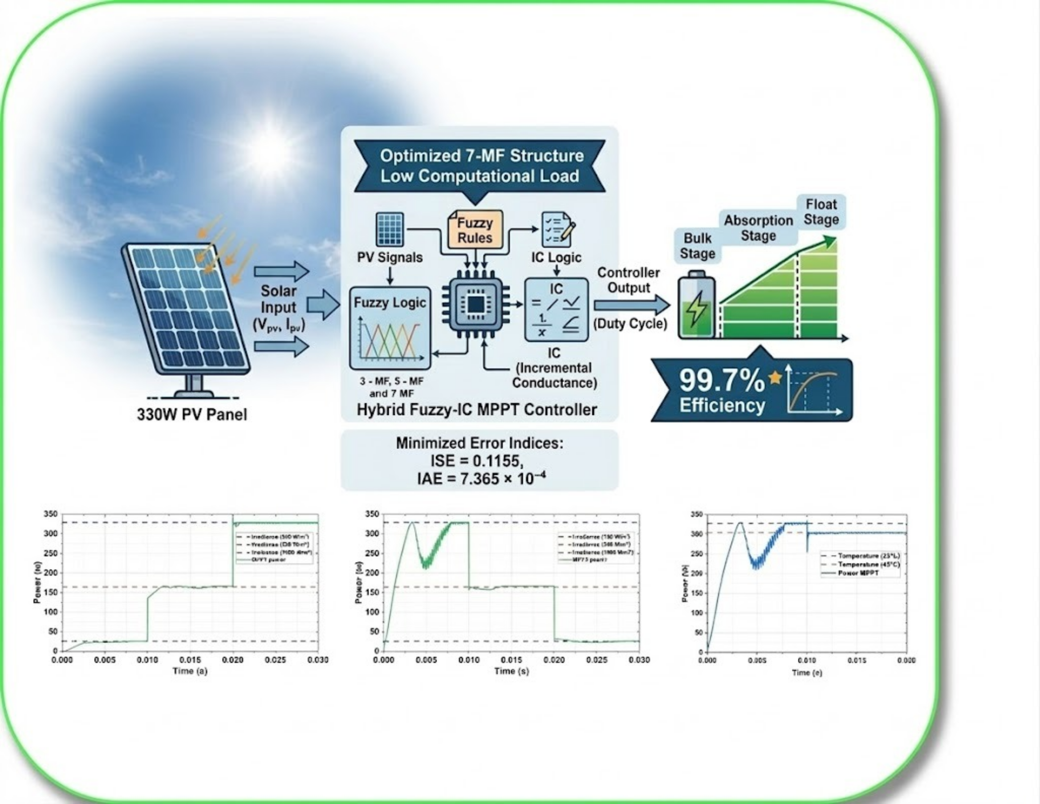
This study presents a hybrid controller that integrates fuzzy logic control and the incremental conductance method. This controller optimizes maximum power point tracking in a 330 W photovoltaic system by designing a step-down DC-DC converter. The study evaluates the impact of the number of membership functions (three, five, and seven) and their distribution using the integral performance indices: Integral Square Error (ISE) and Integral Absolute Error (IAE). The results demonstrate that the seven-function configuration achieved optimal values of 0.1155 and 7.365 ×10⁻⁴, for ISE and IAE respectively. In addition, this configuration achieved an energy efficiency of 99.7%, which is superior to the 98.9% efficiency obtained with three functions in the worst-case scenario. The optimal configuration was subjected to changes in irradiance and temperature to assess its dynamic response robustness. Additionally, an analysis of computational resource consumption reveals that the proposed hybrid controller requires a lower computational load for rule evaluation than three controllers from recent literature. These findings demonstrate the structural efficiency and optimization capability of the proposed system to maximize energy harvesting in photovoltaic panels at a low computational cost.
Keywords:
MPPT
; fuzzy logic control
; incremental conductance
; structural optimization
; photovoltaic systems
; battery charging
1. Introduction
Solar energy can be converted into useful energy through natural processes or technical means. Solar energy is the electromagnetic radiation emitted by the Sun through nuclear fusion reactions in its core. This radiation primarily reaches Earth as visible light, infrared radiation, and ultraviolet radiation. Together, these types of radiation provide light and heat. When this radiation interacts with the surface and atmosphere of Earth, it heats the continents and oceans. This determines weather patterns and enables natural processes, such as photosynthesis. Technologically, solar energy can be converted into usable forms, primarily electricity through the photovoltaic effect and heat through solar thermal absorption. Thus, solar energy manifests as light, heat, and a flow of usable energy that can be harnessed directly or indirectly for human use.
The photovoltaic (PV) solar cell is the core component of a PV energy system. It is a P-N junction diode, and the most commercially available solar cells today are made of silicon. However, copper-cadmium sulfide (CuS/CdS) and gallium arsenide (GaAs) cells are two other types of solar cells that were used in early photovoltaic systems [1]. Over the past two decades, PV cell manufacturing technologies have evolved and improved in performance. Currently, PV cells are produced using crystalline, multicrystalline, thin-film, amorphous, microcrystalline, organic, and multi-junction technologies. The efficiency of crystalline silicon cells has increased to 25.6%. Thin-film and multicrystalline silicon cells have an efficiency range of 10.5% to 21.2%. GaAs-based III-V cells are the most efficient, reaching up to 28.8%. Amorphous and microcrystalline silicon cells are around 11% efficient. Organic thin-film cells have an efficiency of around 11%. For more detailed information, review the study by Green et al. [2], which provides a detailed list of photovoltaic solar cell types and their efficiencies. In another study, Green et al. [3] demonstrated an efficiency of 27.8% for a large-area (134 cm2) n-type silicon cell manufactured by LONGi Green Energy Technology Co. Ltd. and measured in January 2025 by the Solar Energy Research Institute (ISFH). The ISFH is a leading, independent, public research institute in Germany focused on applied solar energy research. LONGi Green Energy Technology Co. Ltd. refers to the cell as a hybrid interdigitated back contact (HIBC) cell with p-type heterojunction and n-type TOPC contacts.
The performance of a PV system depends on the operating conditions and the quality of the solar cell and panel designs. The voltage, current, and power output of a PV panel vary based on solar irradiation levels, temperature, and load current. Different control strategies have been applied to overcome the undesirable effects of these factors on the power output of PV systems. These strategies fall into two main groups: (1) controlling sunlight entering the PV panel and (2) controlling the power output.
In a stand-alone PV system, solar panels serve as the primary source of energy generation. At least one battery or battery bank is necessary to store the captured energy and provide electricity to different systems and devices at night or during periods of low solar radiation. Lead-acid batteries are a good choice for storing energy in stand-alone PV systems because they are maintenance-free. They also offer excellent cost efficiency and are available on the market with a wide range of power ratings [4,5,6]. Since installing a PV system requires a significant investment, it is essential to maximize solar energy use and storage in order to achieve technical and economic sustainability [7]. A solar panel delivers the greatest amount of electrical power when it operates at its maximum power point (MPP). This operating point shifts according to the atmospheric conditions to which the panel is subjected. The MPP must be tracked in all weather conditions. Approaches and techniques based on this principle are known as maximum power point tracking (MPPT) and can increase energy production by 30% to 40% [8]. The MPPT approach uses a direct DC-DC converter to interface the PV array with the battery bank. The objective of the MPPT is to regulate the voltage or current input by controlling the duty cycle of the converter to match the maximum power voltage and current of the PV array under atmospheric conditions. Several types of controls that have been proposed for DC-DC converters in recent years have been used as battery chargers in PV systems [9,10,11,12]. One popular approach is to control the duty cycle of the inverter directly through an MPPT algorithm to extract the maximum instantaneous power from the PV panels, as shown in [13,14]. However, this approach has a drawback. It adds stress to the switches and increases switching losses [15]. Some authors have proposed incorporating PI current and/or voltage control loops to adjust the duty cycle of the converter. This adjustment reduces the time needed for the converter to stabilize, prevents overshoot during oscillation, and enhances the dynamic response of the MPPT, as shown in [16].
Studies by Koutroulis and Kalaitzakis [4] and by Huang [17] have proposed configurations in which the MPPT operates in combination with an on-off type charge control algorithm. In these configurations, the concept and strategy of charge regulation are based on the voltage and state of charge (SoC) of the battery. Clearly, there is an abundance of DC-DC converter controllers for PV applications. However, most studies focus on analyzing the MPPT algorithm and its impact on PV panel efficiency. At least nineteen different MPPT techniques were introduced by 2005 [18]. Conversely, converter control for battery chargers is often overlooked, despite the fact that lead-acid batteries require precise control over their charging and discharging processes to prevent premature aging. According to Enslin et al. [19], this issue is especially important in off-grid PV systems because the battery bank is one of the most expensive components, accounting for 30% of the total investment. But a study by Desconzi et al. [7] reported that the maintenance costs can increase this quantity to 46%. This increase may be primarily due to the inefficient management of battery charging and discharging processes. This can result in the need for premature replacement of the battery [20].
Furthermore, the literature reports that several techniques and algorithms have been used to charge batteries, including constant current, constant voltage, and on-off, among others [17,21,22]. However, a study by Hirech et al. [5] found that these techniques often fail to fully charge the battery and do not protect against premature aging. According to the manufacturers, the two-stage charging method is the most efficient way to restore the full capacity of 12V lead-acid batteries and extend their lifespan.
On the other hand, Nivedha and Vijayalaxmi [21] presented a hybrid MPPT control based on fuzzy logic for PV systems. The MPP was tracked using the fuzzy fractional short-circuit control (FSCC) algorithm whenever changes in atmospheric conditions occurred. When atmospheric conditions remained largely unchanged, the MPP was tracked using the fuzzy perturb and observe (PO) algorithm. They evaluated the following three performance indices for the fuzzy based hybrid control algorithm: integral absolute error (IAE), integral squared error (ISE), and integral time absolute error (ITAE), as well as tracking time. The results showed that the proposed fuzzy-based hybrid MPPT control algorithm outperformed the conventional PO, fuzzy PO, and fuzzy FSCC algorithms in terms of dynamic performance. Various MPPT methods have been used to maximize energy generation in PV panel systems under different climatic conditions. For example, Çakmak et al. [22] proposed a hybrid MPPT algorithm controlled by fuzzy logic, based on the PO algorithm. The fuzzy logic control (FLC) algorithm and the IC MPPT algorithm were simulated in a MATLAB/Simulink environment. Then, the results were evaluated by comparing them with those of other studies [22].
In Melhaoui et al. [23] used an MPPT with a hybrid approach combining IC and FLC. They used the sum of conductance and IC, along with the rate of change, to enhance system performance. Using key performance metrics such as root mean square (RMS), root mean square error (RMSE), and efficiency (, they performed MATLAB/Simulink simulations to evaluate the tracking speed, accuracy, and stability of these algorithms around the MPP. They conducted other evaluations under extreme operating conditions, including abrupt changes in irradiance and sudden load variations, to test the robustness and adaptability of each algorithm [24,25,26].
In this context, this study proposes a hybrid MPPT controller combining IC and FLC . It also evaluates the impact of different positioning schemes and the number of membership functions (three, five, or seven). The performance of the controller was analyzed using the integral error criteria, ISE and IAE. Therefore, a fuzzy control strategy was used to develop the proposed controller for a buck power converter, which was employed as an efficient lead-acid battery charger in an autonomous PV system. This control strategy uses feedback from both the solar panel power and the battery power to regulate the duty cycle of the converter through a pulse width modulator (PWM). The two main objectives of this approach were to maximize the use of available solar energy by using the MPPT with the IC algorithm and to extend the lifespan of the battery bank by precisely controlling the battery charge in two stages. The proposed controller is based on a typical fuzzy cascade structure.
The rest of this paper is organized as follows: Section 2 describes the proposed hybrid MPPT system and the methodology for its evaluation. This section covers the battery charging strategy, fuzzy controller implementation, performance evaluation criteria, and membership function tuning. Section 3 presents the results of the MATLAB/Simulink simulation of the PV system and the MPPT with the proposed hybrid controller. Section 4 discusses the computational load of the proposed controller in relation to existing approaches. Finally, Section 5 summarizes the conclusions of the study..
2. Materials and Methods
This section describes the materials and methods considered in a PV system developed with an IC- and FLC-based hybrid MPPT controller to optimize energy extraction from a solar panel and regulate lead-acid battery charging via a buck-type DC-DC converter. Firstly, the battery charging strategies are detailed. Then, the general block diagram of the MPPT system is presented, along with a DC-DC converter design that considers the response of the solar panel to variations in temperature and irradiance, as well as the parameters provided by the manufacturer. Then, the methodology for evaluating the controller is presented. Next, the implementation of the hybrid MPPT is described. This section explains how the error derived from the IC is calculated and how the FLC is structured. It also includes the input and output membership functions, as well as their associated rules. Lastly, the performance evaluation criteria, the evaluation methodology, and the membership function tuning procedure used in the experimental setup are presented. These criteria ensure efficient and stable MPPT operation.
2.1. Battery Charging Strategy
A control strategy is necessary to fully charge a battery used in PV systems within the permitted current and voltage ranges. The amount of energy generated by the PV panel each day to charge the battery is limited. In this context, many lead-acid battery manufacturers recommend dividing the charging process into three stages: Region 1: initial charge; Region 2: absorption stage; and Region 3: float charge. Figure 1 shows this process.
-
Region 1 initial load:In the low-charge battery condition, the battery voltage can be between its minimum allowed value and its maximum overcharge value . In this case, the MPPT algorithm must be executed to extract the maximum power from the panel. At this stage, the charging current is limited to the maximum deep charging current . This current corresponds to a percentage of the battery capacity to prevent overheating and premature wear. At this stage, the battery capacity is generally recovered to between 80% and 90%.
-
Region 2 absorption stage:Entry into region 2 is clearly indicated when the battery voltage reaches the maximum voltage.In this region, voltage control is applied, with the set point adjusted to .
-
Region 3 float charge:When the value of falls below the minimum charging current , the controller reduces its set point to the float voltage value . This voltage reference generates a very small charging current, which is sufficient only to compensate for self-discharge. To prevent deep discharge above the value permitted by the manufacturer, the control acts on a disconnect relay whenever is lower than the minimum permitted voltage and no charging energy is available.
However, the manufacturer of the battery model “CALE-SOLAR 31T” used in this study recommends a two-stage charging strategy: 1) initial load (fast charging) and 2) float charge (maintenance stage). Therefore, although the three-region model is presented for a general understanding of the process, a fuzzy controller was designed to implement the control strategy, following the two-stage approach adapted to the battery in question. Additionally, to ensure that lead-acid batteries are charged fully, quickly, and safely, a battery protection stage has been added to the float charger’s design, featuring two conditions based on battery voltage and .
2.2. MPPT System and Converter Design
Figure 2 shows a block diagram of a system containing the most important parts for converting solar energy into electrical energy and storing it in a battery via a DC-DC step-down converter.
It starts with the solar panel, which delivers a voltage signal and current . These variables are measured by a voltage and current sensor and sent to the MPPT control block. The energy generated by the panel is conditioned by a Buck-type DC-DC converter, whose main switching element is a MOSFET. The duty cycle of the MOSFET is regulated by a PWM signal generated by the MPPT algorithm. In parallel, the battery voltage is measured and the is estimated. These variables act as monitoring conditions to protect the battery bank or battery.
The MPPT block processes the electrical variables , , , and . It also generates the PWM signal that adjusts the converter’s duty cycle through a MOSFET transistor, forcing the panel to operate at its MPP.
2.3. Evaluation Methodology
The following four steps describe a procedural method for evaluating the design of a hybrid MPPT.
- 1.
-
Electrical characteristics of the PV system. The current-voltage () and power-voltage () curves of the PV system reveal that external factors such as irradiance and temperature significantly influence output power and efficiency. The power output of the system is directly proportional to irradiation, while its relationship with temperature is inversely proportional. However, a DC-DC converter and the control system topology can track changes in the MPP caused by temperature or irradiation fluctuations, as shown in Figure 3 and Figure 4.The module used in this study is a polycrystalline EPL33024 panel. Its main parameters are shown in Table 1.These features allow you to model the behavior of the system under different environmental conditions in MATLAB/Simulink.
- 2.
-
DC-DC converter design. The output power of a PV system varies according to changes in atmospheric conditions. Therefore, a DC-DC converter is used to maintain the output current and voltage of the PV source at a MPP. The graphical representation of a DC-DC step-down converter is shown in Figure 5. The converter changes the input voltage , which is DC, to an output voltage . A control signal nown as a PWM signal is applied, which remains high (1) for a designated period “ON” and low (0) for a period “OFF”; in other words, it regulates the duty cycle. A DC-DC converter is used to maintain the current and output voltage of the PV system, as the output power of the system varies with atmospheric conditions. A step-down buck converter was selected because the panel voltage is higher than the nominal battery voltage (12 V).The DC-DC converter operates in continuous conduction mode (CCM) under the assumptions of ideal switching conditions and negligible losses. Under these assumptions, the voltage conversion ratio of the step-down converter is given by Eq. 1.The DC-DC converter is designed to act as an interface between the PV panel and the battery. This allows the MPPT algorithm to regulate the operating point of the PV system by controlling the duty cycle. Therefore, when designing the converter, it is essential to select parameters that ensure a rapid dynamic response and stable operation of the PV panel under varying environmental conditions.The passive components (inductor and capacitor) were designed considering the current ripple, voltage ripple, and nominal operating conditions specifications, which are shown in Table 2. Assuming a variation in the input voltage, the duty cycle range is determined to ensure proper operation under different irradiance conditions. The battery used is 12 V and 100 model “CALE-SOLAR 31T”, considering two charging stages:Region 1. Up to 14.8 VRegion 3. Reduction to 13 Vwhere is the switching frequency of the MOSFET. Therefore, the current that the semiconductors must switch and block is presented in Eq. 2, R is given by Eq. 3, and the operating interval of the duty cycle is given by Eq. 4.Assuming that the supply voltage is given as = 37.87 V , then 0.3256 ≤ D ≤ 0.4885.On the other hand, knowing that 2.23 A and considering that,Therefore, when D = 0.3256, L = 894.86 , and when D = 0.4885, L = 679 .
- 3.
-
General diagram of the MPPT system. PV systems exhibit nonlinear behavior due to continuous variations in irradiance and temperature. These changes alter the MPP, which corresponds to the operating condition in which the panel delivers its maximum power. To ensure that the system operates near this optimal point, the MPPT algorithms are used, which adjust the converter dynamically to maintain the panel in the MPP. Within the MPPT block shown in Figure 6, the hybrid strategy was implemented, in which FLC receives as inputs , , , and . The controller generates a preliminary D based on fuzzy rules, which improves dynamics and reduces oscillations around the MPP.In addition, to ensure the operational integrity of the CALE-SOLAR 31T battery (12 V, 100 Ah), the D of the fuzzy controller is conditioned by two cascaded logic multipliers, as illustrated in Figure 6. Although the panel voltage is a fundamental input for the control algorithm, it is not considered a safety condition. The constraints focus exclusively on the output node to protect the battery and any load system that depends on it. The first constraint stipulates that the output voltage must satisfy the condition V, a threshold defined by the manufacturer for the float charging region that prevents prolonged chemical stress. The second constraint ensures that the is less than 100%, which inhibits energy transfer once full nominal capacity is reached. If either condition is false (logical value 0), the Boolean multiplication operation cancels the duty cycle (). Finally, the PWM generator produces a switching signal that is applied to the buck converter’s MOSFET. The MOSFET stops immediately if the preconditions are not met, ensuring safe and efficient load management.
- 4.
-
Implementation of FLC with IC. This block in Figure 7 shows how the IC method is implemented in combination with fuzzy logic.In this approach, the MPPT is identified using the P-V characteristic curve of the PV panel. This algorithm continuously measure the current and voltage of the PV panel to calculate the generated power as shown in Eq. 7.The error occurring in the system and its variation are subsequently calculated and used as the actual for fuzzy logic, as illustrated in Eq. 12.Therefore, it can be considered that,The performance of the proposed algorithm is based on the nonlinear characteristic of the power-voltage (P-V) curve of the PV panel. The derivative of power with respect to voltage, defined as , is selected as the input error signal for the fuzzy controller for the following thermodynamic and operational reasons:
- (a)
-
Maximum power condition:Mathematically, the MPP occurs when the slope of the P-V curve is zero (). Therefore, any value other than zero represents an “error” or deviation from the optimum operating point.
- (b)
-
Identification of the region of operation:The sign of the derivative indicates which side of the curve the system is on:
- If : The system operates to the left of the MPP (constant current region). The controller must increase the voltage.
- If : The system operates to the right of the MPP (constant voltage region). The controller must decrease the voltage.
- (c)
-
Relationship with IC:This input links fuzzy logic with the IC method, where the condition is equivalent to . By using the derivative as input, the fuzzy system not only detects the direction of the error, but the magnitude of the slope allows the controller to dynamically adjust the duty cycle: large slopes require larger steps, while slopes close to zero activate fine steps to reduce oscillations in the steady state.
Fuzzy rule-based systems translate qualitative, vague, and imprecise human experiences and judgments into control rules. Membership functions are empirically determined based on given guidelines through trial and error. The performance of a conventional controller is typically specified by the steady-state behavior of a closed-loop system (steady-state error) and the transient response (transient error) of a feedback control system. Similarly, the rules of a fuzzy controller can also be specified by the desired steady-state and transient responses, expressed in fuzzy terms such as fast rise time, minimum overshoot, steady-state error, and transient error.
The objective is to generate fuzzy rules or membership functions without relying on an experienced human operator with in-depth knowledge of controlling the plant in question. Although the original purpose of using fuzzy logic in control systems was to incorporate the human contribution, an experienced operator may not always be available. In these cases, the knowledge of the operator must be recreated through a learning process in which the input/output parameters of the plant are measured and recorded as input/output time vectors. One type of learning occurs in the presence of a performance evaluator (J) that indicates the necessary structural or parameter modifications compared to a predetermined standard..
2.4. FLC Implementation
A Mamdani-type FLC is used for the implementation of the MPPT algorithm due to its intuitive structure and wide application in nonlinear systems such as PV systems. The Mamdani fuzzy controller consists of four main stages: 1) definition of the discourse universe, 2) fuzzification, 3) inference, and 4) defuzzification [27].
- 1.
- Definition of the discourse universe: The input domain is defined in the interval (-10, 10) and represents the range of a power membership triangular function The output domain is defined in the interval (0, 0.8) and represents the range of a duty cycle
- 2.
-
Fuzzification is the process of making a precise quantity fuzzy and representable by a membership function. The input membership functions to the fuzzy controller can be generated from three, five, and seven membership functions based on the generalized membership function presented in Table 3, where the parameters of the base edges are given by an with . The membership function has maximum degrees of membership at ± b0, ±b1, ±b2, and ±b3.The degree of membership is a number in the interval [0,1] that indicates the importance of a rule within a set of rules.
- 3.
-
Mamdani inference. In the inference stage, the general form of the linguistic rules is: If premise, then consequent.In this study, it is denoted as follows:If E is , then D isHere, and represent the fuzzy sets corresponding to the input and output membership functions, respectively.Note that the AND operator is not used since only a single input is required for the membership functions. However, the AND operator is necessary when using two or more inputs to proceed to the next stage: defuzzification. According to Passino et al. [27], this is directly related to the computational load of the software used for the simulations.Table 4 shows the rules defined for this study. The premises are related to the inputs of the fuzzy controller and are located on the left side of the rules. The consequences are associated with the fuzzy output and are on the right side of the rules. The rule base includes the operations that enable the fuzzy system to generate a single output by connecting the sets of fuzzy inputs and outputs. The rule base is applied to the membership function obtained according to Mamdani inference.A fuzzy output set is generated for each rule, which is associated with the variation in the DC-DC converter duty cycle.
- 4.
-
Defuzzification. This study uses the centroid method because it is widely used due to its simplicity and allows for the calculation of a precise numerical value to adjust the duty cycle. This centroid method is expressed by Eq. 14:Assuming that is the actual output value from the fuzzy system, represents the center of the fuzzy output set area, and s the membership function associated with each rule.The centroid method was chosen because it provides a smooth and continuous response, which is crucial for MPPT applications where oscillations around the MPP must be minimized. The Mamdani fuzzy controller dynamically adjusts the converter’s duty cycle, ensuring efficient tracking of the MPP despite variations in irradiance and temperature.
2.5. Performance Evaluation Using Error Indices
Evaluation criteria (error metrics): One metric is the ISE, which is given by Eq. 15. This performance index assigns greater weight to large errors and less weight to small ones.
The system is optimal if the value is the minimum of this integral. The IAE criterion evaluates cumulative performance as defined in Eq. 16.
2.6. Membership Function Tuning Based on Performance Indices and Experiment Setup
As illustrated in Figure 10, the membership functions are adjusted by slightly expanding or shifting them. This procedure highlights the rules that contributed significantly to the fuzzy result and those that contributed less.
Although adjusting the contribution weights of the rules can move the central control region of a fuzzy controller in response to changes in the input, changing the weights alone is insufficient for rapid multidimensional adaptation.
Therefore, the proposed changes to the simulations involve assigning different values to the parameters of the membership functions in order to demonstrate their effects on evaluation criteria J1 and J2. A low value for the evaluation criteria indicates a reduction in error over time. Table 5 illustrates this effect.
Table 5 presents three adjustments for three experiments with three, five, and seven power error triangular membership functions.
Note that Figure 10, Figure 11, and Figure 12 only show the positive membership functions starting with (CZ) for ease of visualization in the graph, but the negative membership functions should also be considered, as shown in Figure 8 (SN, MN, and HN), according to Table 5.
Experiment 1 was conducted with adjustments 1, 2, and 3 according to Table 5. The graphical representation is shown in Figure 11. The membership functions (CZ and SP) are defined in the positive values of .
3. Results
This section presents the results of the MATLAB/Simulink simulation of the 330 W polycrystalline PV system, “EPL33024”, and the MPPT with the proposed hybrid controller, as shown in Figure 2, in accordance with the PV system parameters shown in Table 1 and the R, L, C, and D parameters calculated for the DC-DC step-down converter.
The analysis is divided into four phases: 1) The J1 and J2 indices for each test should be obtained according to Table 5 and the Eqs. 15 and 16; 2) Select the best fit for the membership functions in each of the three tests. This will ensure that the performance indices J1 and J2 of the fuzzy controller are minimized. It will also show the time response of the MPPT power for each selected setting; 3) Calculate the efficiency according to the three settings selected in the previous point; and 4) Validate the robustness of the energy generated by the MPPT. Select the setting that minimizes J1 and J2 and has the highest efficiency in the face of changes in environmental conditions. Changes in environmental conditions include increases or decreases in solar irradiation (1000, 500, and 100 ) and temperature changes (25 °C and 45 °C).
3.1. Obtaining the J1 and J2 Indices
3.2. Selection of Membership Function Settings
According to Table 6 and Figure 14, for the 3FM (functions membership) test, the setting that minimizes J1 and J2 is setting number two, with J1 = 0.1373 and J2 = 8.591. For the 5FM test, setting number three was selected, with J1 = 0.1255 and J2 = 8.129. For the 7FM test, setting number three minimizes J1 and J2, with values 0.1155 and 7.365, respectively.
Figure 15 shows the dynamic behavior of the MPPT output power (test 3FM, setting 2) under 1000 and 25 °C conditions. As can be seen, the power follows the 330 W reference and reaches a steady state at approximately 0.008 seconds (S). During the transient period, significant disturbances occur between 0.0045 s and 0.006 s, during which pronounced ripples and a minimum power value close to 60 W are recorded.
Figure 16 shows the dynamic behavior of the MPPT output power (5FM, setting 3) under an irradiance of 1000 W/m² and a temperature of 25 °C. The system reaches a reference power of 330 W approximately after 0.008 s. During the transient stage, an initial maximum overshoot occurs at 0.003 s, followed by moderate ripple oscillations between 0.004 s and 0.006 s. The minimum power value does not fall below 195 W during this time. Finally, the system enters a steady state with moderate ripple.
Figure 17 shows the dynamic performance of the MPPT output power (7FM, setting 3) under 1000 and 25 °C conditions. The system exhibits an initial overshoot, reaching the 330 W reference at 0.003 s. This is followed by an adjustment stage with a controlled power drop to 210 W at 0.0048 s. Minimal transient ripple, less than that observed in the 3FM and 5FM tests, is seen from 0.004 s to 0.0075 s. The system then stabilizes definitively at the 330 W reference value from 0.008 s onward.
3.3. MPPT Efficiency Calculation
The efficiency of the MPPT is calculated using Eq. 17, under conditions of 1000 and 25 °C. According to Table 1, under these conditions, the MPPT theoretically provides 330 W. The settings that minimize indices J1 and J2 are selected in accordance with Section 3.2.
3.4. Response to Variations in Irradiance and Temperature
According to Figure 14, Table 6 and Table 7, the adjustment that minimizes J1 = 0.1155, J2 = 7.365 and presents the highest efficiency of 99.7% is the 7 FM adjustment 3. The response of this adjustment is evaluated with stepped changes in irradiance: 1) Upward with three stepped increases of 100, 500, and 1000 , and 2) Downward with three stepped decreases of 1000, 500, and 100 . These changes simulate environmental conditions such as the sun rising and reaching maximum irradiance in the morning, then decreasing to minimal irradiance in the afternoon as the sun sets, or the passage of clouds or clearing skies.
Figure 18 shows the output power of the MPPT as irradiance increases. The MPPT provides 28.82 W at 100 , 164.77 W at 500 , and 329.01 W at 1000 , which is consistent with the graphs provided by the panel manufacturer in Figure 4.
Figure 19 shows the output power of the MPPT as irradiance decreases. The MPPT provides 329.01 W at 1000 W/m2, 164.77 W at 500 W/m2, and 28.82 W at 100 W/m2.
4. Discussion
This paper proposes an FLC hybrid with an IC called “controller 4”, which is a fuzzy system with one input and one output. Both are configured with three, five, or seven membership functions. To evaluate computational resource consumption, it is compared with three additional proposals: Controller 3 ([21]), which uses two inputs and one output, with three membership functions each; Controller 2 ([23]) uses two inputs and one output with five membership functions each; and Controller 1 ([22]) uses two inputs and one output with seven membership functions per variable. All four controllers implement the Mamdani-type inference method. To determine which controller requires the greatest computational load, the three critical stages of this process are analyzed: fuzzification, rule evaluation, and defuzzification. Although controller 3 has fewer membership functions per input, the ‘dimension explosion’ that occurs when adding a second input makes the process more computationally intensive than having a single input with more functions. Controller 4 consumes the fewest computational resources of the four mentioned. In fuzzy logic, the computational load depends not only on how many membership functions a variable has, but also on how they are combined with one another. A detailed comparison of the four cases is provided in Table 8.
According to Passino et al. [27], the technical reasons for low consumption in controller 4 are as follows:
- 1.
- Exponential growth of rules: The number of rules can be calculated using the formula , where M is the number of membership functions and n is the number of inputs. As you can see, switching from a single-input to a dual-input configuration increases the number of rules from 5 to 25 when comparing controller 4 with the 5-FM test to controller 2. This increases the processing workload fivefold during the inference process.
- 2.
-
Conjunction cost (antecedents):
- In controller 4, the strength of the rule is simply the value of the input.
- For each rule in controllers 1, 2, and 3, the processor must perform an intersection operation (usually a minimum). For controller 1, this requires performing at least 49 additional logical comparisons per execution cycle.
- 3.
-
Mamdani aggregation and defuzzification: The Mamdani method requires calculating the area of the union of all truncated output functions.
- Controller 4 must only overlay and average up to 3, 5, or 7 areas.
- Controller 1 must process the overlap of up to 49 potential areas, which makes the calculation of the centroid extremely costly in terms of clock cycles and memory usage.
5. Conclusions
This study presents an optimal hybrid MPPT designed to combine FLC and the IC method for PV systems. The controller was applied to a DC-DC step-down converter operating in CCM with a 330 W PV module and battery storage. The study examines how the number and distribution of membership functions influence the dynamic behavior of the MPPT based on fuzzy logic. Three configurations with different positioning schemes are evaluated: three, five, and seven triangular membership functions. System performance was evaluated using the ISE and IAE indices. The results show that increasing the number of membership functions improves the approximation capability of nonlinear PV characteristics. However, the performance improvement depends heavily on the proper distribution of the membership functions. The seven-member configuration achieved the lowest error indices with an optimized fit. Meanwhile, the five-member configuration provided an adequate balance between tracking accuracy and computational complexity. These findings underscore the significance of structural optimization in the design of a fuzzy, data-based MPPT for the efficient extraction of PV energy. After obtaining the optimal design, validation simulations are performed using MATLAB-Simulink to demonstrate the performance of the proposed control system. The results show that the arrangement of the seven membership functions with adjustment 3, as shown in Figure 12, is the best. It has a performance index of 0.1155 and 7.365 for J1 and J2, respectively. In addition, this methodology can help engineers develop expert knowledge to optimize and stabilize a set of membership functions, achieving the MPP in PV solar panels. The simulations for the best performance index are robust.This is evident from simulations with variations in irradiation of 1000, 500, and 100 , which demonstrate that the maximum theoretical value provided by the solar panel manufacturer is achieved for these values. Based on the discussion above and the computational load required by each controller (logical operations used for inference in the rule base), the order of resource consumption for each controller, from lowest to highest consumption, is: Controller 4 < controller 3 < controller 2 < controller 1. Controller 4, proposed in this study, is by far the least resource-intensive, as it requires nearly ten times fewer rule evaluations than controller 1.
Nomenclature
| Symbol | Description |
| PV | Photovoltaic |
| CuS/CdS | Cooper-Cadmium sulfide |
| GaAs | Gallium arsenide |
| LONGi | Green energy technology Co. Ltd |
| HIBC | Hybrid interdigitated back contact |
| MPP | Maximum power point |
| MPPT | Maximum power point tracking |
| DC-DC | Direct current-direct current |
| SoC | State of charge |
| FLC | Fuzzy logic control |
| FSCC | Fuzzy fractional short-circuit control |
| PO | Perturb and observe |
| IAE | Integral absolute error |
| ISE | Integral squared error |
| ITAE | Integral time absolute error |
| IC | Incremental conductance |
| RMS | Root mean square |
| RMSE | Root mean square error |
| PWM | Pulse width modulation |
| CCM | Continuous control mode |
| D | Duty cycle |
| Efficiency | |
| Degree of membership functions |
Author Contributions
Conceptualization: E.R.-C., O.J.-R. and D.G.-R.; methodology: E.R.-C. and O.J.-R.; software: E.R.-C. and D.G.-R.; validation: O.J.-R., D.A.-T., D.G.-R. and R.V.-M.; formal analysis: D.A.-T.; investigation: E.R.-C. and D.G.-R.; resources: O.J.-R. and R.V.-M.; data curation: E.R.-C., D.G.-R., and D.A.-T.; writing—original draft preparation: E.R.-C., D.G.-R., and O.J.-R.; writing—review and editing: R.V.-M., D.G.-R., E.R.-C., O.J.-R.,and D.A.-T.; visualization: O.J.-R., D.A.-T., and R.V.-M.; supervision: O.J.-R., D.A.-T., and R.V.-M.; project administration, O.J.-R., D.A.-T., and R.V.-M.; funding acquisition, O.J.-R. and R.V.-M. All authors have read and agreed to the published version of the manuscript.
Funding
This research was funded by the Instituto Politécnico Nacional under grant number MULTI-2026-0038.
Institutional Review Board Statement
Not applicable.
Informed Consent Statement
Not applicable.
Data Availability Statement
Data will be made available upon request.
Acknowledgments
Ezequiel Rincón-Canalizo (CVU-2063199), D. Aguilar-Torres (CVU-829790) and D. Gutiérrez-Rosales (CVU-1269306) are grateful for the grant provided by Secretaría de Ciencia, Humanidades, Tecnología e Innovación (SECIHTI, México). The authors would like to thank Dr. Araujo-Vargas Ismael for his valuable technical guidance and expertise in Power Electronics, particularly regarding the design and optimization of the buck converter stage used in this study.
Conflicts of Interest
The authors declare no conflicts of interest.
References
- Buresch, M.E. Photovoltaic energy systems; Bibliography; McGraw-Hill: New York [u.a.], 1983; pp. 233–236. [Google Scholar]
- Green, M.A.; Emery, K.; Hishikawa, Y.; Warta, W.; Dunlop, E.D. Solar cell efficiency tables (version 45). Progress in Photovoltaics: Research and Applications 2015, 23, 1–9. [Google Scholar] [CrossRef]
- Green, M.A.; Dunlop, E.D.; Yoshita, M.; Kopidakis, N.; Bothe, K.; Siefer, G.; Hao, X.; Jiang, J.Y. Solar cell efficiency tables (version 66). Progress in Photovoltaics: Research and Applications; 2025. [Google Scholar]
- Koutroulis, E.; Kalaitzakis, K. Novel battery charging regulation system for photovoltaic applications. IET Electric Power Applications 2011, 151, 191–197. [Google Scholar] [CrossRef]
- Hirech, K.; Melhaoui, M.; Yaden, F.; Baghaz, E.; Kassmi, K. Design and realization of an autonomous system equipped with a charge/discharge regulator and digital MPPT command. Energy Procedia 2013, 42, 503–512. [Google Scholar] [CrossRef]
- Salas, V.; Olías, E.; Barrado, A.; Lázaro, A. Review of the maximum power point tracking algorithms for stand-alone photovoltaic systems. Solar Energy Materials and Solar Cells 2006, 90, 1555–1578. [Google Scholar] [CrossRef]
- Desconzi, M.; Beltrame, R.; Rech, C.; Schuch, L.; Hey, H. Photovoltaic stand alone power generation system with multilevel inverter. In Proceedings of the International Conference on Renewable Energies and Power Quality (ICREPQ), Las Palmas, Spain, 2010. [Google Scholar]
- Taghvaee, M.; Radzi, M.; Moosavain, S.; Hashim, H.; Hamiruce, M. A current and future study on non-isolated DC–DC converters for photovoltaic applications. Renewable and Sustainable Energy Reviews 2013, 17, 216–227. [Google Scholar] [CrossRef]
- Singh, D.K.; Akella, A.K.; Manna, S. A novel robust maximum power extraction framework for sustainable PV system using incremental conductance based MRAC technique. Environmental Progress & Sustainable Energy 2023, 42, e14137. Available online: https://aiche.onlinelibrary.wiley.com/doi/pdf/10.1002/ep.14137. [CrossRef]
- Kumar, M.; Panda, K.P.; Rosas-Caro, J.C.; Valderrábano-González, A.; Panda, G. Comprehensive Review of Conventional and Emerging Maximum Power Point Tracking Algorithms for Uniformly and Partially Shaded Solar Photovoltaic Systems. IEEE Access 2023, 11, 31778–31812. [Google Scholar] [CrossRef]
- Mienye, I.D.; Sun, Y. A Survey of Ensemble Learning: Concepts, Algorithms, Applications, and Prospects. IEEE Access 2022, 10, 99129–99149. [Google Scholar] [CrossRef]
- Abbass, M.J.; Lis, R.; Saleem, F. The Maximum Power Point Tracking (MPPT) of a Partially Shaded PV Array for Optimization Using the Antlion Algorithm. Energies 2023, 16. [Google Scholar] [CrossRef]
- Liu, S.; Guo, X.; Wang, L.; Li, S. A novel maximum power point tracking control method with variable weather parameters for photovoltaic systems. Solar Energy 2013, 97, 529–536. [Google Scholar] [CrossRef]
- Ioannou, A.; Kofinas, P.; Papadakis, G.; Alafodimos, C. A direct adaptive neural control for maximum power point tracking of photovoltaic system. Solar Energy 2015, 115, 145–165. [Google Scholar] [CrossRef]
- Kislovski, A. Dynamic behavior of a constant frequency buck converter power cell in a photovoltaic battery charger with a maximum power tracker. In Proceedings of the Fifth Annual Applied Power Electronics Conference and Exposition. IEEE, 1990; pp. 212–220. [Google Scholar]
- Artal-Sevil, J.S.; Coronado-Mendoza, A.; Haro-Falcón, N.; Domínguez-Navarro, J.A. High-Efficiency Partial-Power Converter with Dual-Loop PI-Sliding Mode Control for PV Systems. Electronics 2025, 14. [Google Scholar] [CrossRef]
- Huang, C.C.; Kuo, P.K. Implementation of a stand-alone photovoltaic lighting system with MPPT, battery charger and high brightness LEDs. Proceedings of the 2005 International Conference on Power Electronics and Drives Systems. IEEE 2005, Vol. 2, 1601–1605. [Google Scholar]
- Esram, T.; Chapman, P.L. Comparison of photovoltaic array maximum power point tracking techniques. IEEE Transactions on Energy Conversion 2007, 22, 439–449. [Google Scholar] [CrossRef]
- Enslin, J.H.; Wolf, M.S.; Snyman, D.B.; Swiegers, W.J. Integrated photovoltaic maximum power point tracking converter. IEEE Transactions on Industrial Electronics 1997, 44, 769–773. [Google Scholar] [CrossRef]
- Samuel, A.; Torrico-Bascope, R.; Antunes, F.; Mineiro, E. Stand-alone photovoltaic system using an UPS inverter and a microcontrolled battery charger based on a boost converter with a 3 state-commutation cell. In Proceedings of the 32nd Annual Conference on IEEE Industrial Electronics. IEEE, 2006; pp. 4381–4386. [Google Scholar]
- Nivedha, S.; Vijayalaxmi, M. Performance Analysis of Fuzzy based Hybrid MPPT Algorithm for Photovoltaic system. In Proceedings of the IEEE Xplore, September 2021. [Google Scholar]
- Çakmak, F.; Aydoğmuş, Z.; Tür, M.R. Analyses of PO-Based Fuzzy Logic-Controlled MPPT and Incremental Conductance MPPT Algorithms in PV Systems. Energies 2025, 18, 233. [Google Scholar] [CrossRef]
- Melhaoui, M.; Rhiat, M.; Oukili, M.; Atmane, I.; Hirech, K.; Bossoufi, B.; Almalki, M.M.; Alghamdi, T.A.; Alenezi, M. Hybrid fuzzy logic approach for enhanced MPPT control in PV systems. Scientific Reports 2025, 15, 19235. [Google Scholar] [CrossRef] [PubMed]
- Nataraj, C.; et al. Comparative analysis of direct coupling and MPPT control in standalone PV systems for solar energy optimization to meet sustainable building energy demands. Scientific Reports 2024, 14, 22924. [Google Scholar] [CrossRef] [PubMed]
- Zemmit, A.; et al. GWO and WOA variable step MPPT algorithms-based PV system output power optimization. Scientific Reports 2025, 15, 7810. [Google Scholar] [CrossRef] [PubMed]
- Wandhare, R.; Agarwal, V. Novel integration of a PV-wind energy system with enhanced efficiency. IEEE Transactions on Power Electronics 2015, 30, 3638–3649. [Google Scholar] [CrossRef]
- Passino, K.M.; Yurkovich, S.; et al. Fuzzy control; Addison-wesley Reading, MA, 1998; Vol. 42. [Google Scholar]
Figure 1.
Battery charging regions.

Figure 2.
General block diagram of the MPPT system.

Figure 3.
Characteristics of P vs. V and I vs. V as temperature changes.

Figure 4.
Characteristics of P vs. V and I vs. V with changes in irradiance.

Figure 5.
Electrical diagram of the step-down converter.

Figure 6.
Diagram of the system control and conditioning logic.

Figure 7.
Block diagram of the hybrid IC–fuzzy MPPT controller.

Figure 8.
Graphical representation of an input to the fuzzy controller.

Figure 9.
Graphical representation of an output to the fuzzy controller.

Figure 10.
Adjusting the width of the membership function.

Figure 11.
Two membership functions with positive input values.

Figure 12.
Three membership functions with positive input values.

Figure 13.
Four input membership functions with positive input values.

Figure 14.
Results of membership function tests and their performance indices.

Figure 15.
MPPT response in the 3FM test, setting 2.

Figure 16.
MPPT response in the 5FM test, setting 3

Figure 17.
MPPT response in the 7FM test, setting 3

Figure 18.
MPPT response increases with variations in the 7FM test, setting 3.

Figure 19.
MPPT response decreases with variations in the 7FM test, setting 3.

Figure 20.
MPPT response to temperature variations in the 7FM test, setting 3.


Table 1.
STC Conditions and module parameters considering 1000 W/m2 at 25 °C.
| STC conditions | Value |
|---|---|
| Maximum power () | 330 W |
| Power tolerance | 0 to 5 W |
| Module efficiency | 17.01% |
| Maximum voltage capacity () | 37.87 V |
| Maximum current capacity () | 8.71 A |
| Open circuit voltage () | 46.79 V |
| Short circuit current () | 9.18 A |
| Temperature coefficient () | -0.31% / °C |
| Module cells () | 72 |
| Operating temperature range | -45°C to 85 °C |
Table 2.
Electrical parameters and design specifications of the DC-DC converter.
| Electrical parameters | Design value |
|---|---|
| 37.87 V ± 20% | |
| 14.80 V | |
| 330 W | |
| 0.1 V | |
| 10% | |
| 5kHz |
Table 3.
Rank in discourse for membership functions.
| Name and symbol | Rank in discourse |
|---|---|
| High negative (HN) | -a6, -b3, -a7 |
| Medium negative (MN) | -a4, -b2, -a5 |
| Small negative (SN) | -a2, -b1, -a3 |
| Center Zero (CZ) | -a1, b0, a1 |
| Small Positive (SP) | a2, b1, a3 |
| Medium Positive (MP) | a4, b2, a5 |
| High Positive (HP) | a6, b3, a7 |
Table 4.
Table of fuzzy rules for MPPT.
| ID | Fuzzy rule |
|---|---|
| 1 | if E is HN then D is HP |
| 2 | if E is MN then D is MP |
| 3 | if E is SN then D is SP |
| 4 | if E is CZ then D is CZ |
| 5 | if E is SP then D is SN |
| 6 | if E is MP then D is MN |
| 7 | if E is HP then D is HN |
Table 5.
Membership function adjustments
| Membership function | Adjustment 1 | Adjustment 2 | Adjustment 3 |
|---|---|---|---|
| CZ, SP | b0 = 0, a1 = 3.33 a2 = 3.33, b1 = 6.66 a3 = 9.99 | b0 = 0, a1 = 5 a2 = 0, b1 = 5 a3 = 10 | b0 = 0, a1 = 0.5 a2 = 0.2, b1 = 0.8 a3 = 10 |
| CZ, SP, MP | b0 = 0, a1 = 2, a2 = 2 b1 = 6.66, a3 = 9.99 a4 = 6, b2 = 8, a5 = 10 | b0 = 0, a1 = 3.33 a2 = 0, b1 = 3.33 a3 = 6.66, a4 = 3.33 b2 = 6.66, a5 = 10 | b0 = 0, a1 = 0.5 a2 = 0, b1 = 0.8 a3 = 2, a4 = 1.5 b2 = 6.5, a5 = 10 |
| CZ, SP, MP, HP | b0 = 0, a1 = 1.425 a2 = 1.425, b1 = 2.85 a3 = 4.275, a4 = 4.275 b2 = 5.7, a5 = 7.125 a6 = 7.125, b3 = 8.55 a7 = 10 | b0 = 0, a1 = 2.85 a2 = 0, b1 = 2.85 a3 = 5.7, a4 = 2.85 b2 = 5.7, a5 = 8.55 a6 = 5.7, b3 = 8.55 a7 = 10 | b0 = 0, a1 = 0.2 a2 = 0, b1 = 0.8 a3 = 2.5, a4 = 1.5 b2 = 4.5, a5 = 8 a6 = 3.5, b3 = 7 a7 = 10 |
Table 6.
Performance comparison: ISE and IAE results.
| Test | Number of adjustment | ISE () | IAE () |
|---|---|---|---|
| 3 membership functions | Adjustment 1 | 0.1379 | 8.718 |
| Adjustment 2 | 0.1373 | 8.591 | |
| Adjustment 3 | 0.1374 | 8.68 | |
| 5 membership functions | Adjustment 1 | 0.1298 | 8.464 |
| Adjustment 2 | 0.1243 | 8.312 | |
| Adjustment 3 | 0.1255 | 8.129 | |
| 7 membership functions | Adjustment 1 | 0.1412 | 8.744 |
| Adjustment 2 | 0.126 | 8.435 | |
| Adjustment 3 | 0.1155 | 7.365 |
Table 7.
Efficiency values obtained for the selected settings.
| Adjustment | |
|---|---|
| 3 FM adjustment 2 | 98.9 |
| 5 FM adjustment 3 | 99.3 |
| 7 FM adjustment 3 | 99.7 |
Table 8.
Comparison of computational complexity based on the algorithms used and the FLC configuration between the proposed work and recent literature.
Table 8.
Comparison of computational complexity based on the algorithms used and the FLC configuration between the proposed work and recent literature.
| Feature | Controller 1 [22] | Controller 2 [23] | Controller 3 [21] | Controller 4 This work |
|---|---|---|---|---|
| MPPT algorithm | FLC+PO | FLC+IC (SInC/CSI) | FLC+PO+FSCC | FLC hybrid+IC |
| Configuration (Fuzzification) | 2 inputs (7 MF) | 2 inputs (5 MF) | 2 inputs (3 MF) | 1 input (3 MF), 1 input (5 MF), 1 input (7 MF) |
| Number of rules in the rule base | 49 () | 25 () | 9 () | 3 (), 5 (), 7 () |
| Logical operations (AND) | 49 | 25 | 9 | 0 |
| Output complexity | Very High (7 MF) | High (5 MF) | Medium (3 MF) | Removed (5 MF) |
Disclaimer/Publisher’s Note: The statements, opinions and data contained in all publications are solely those of the individual author(s) and contributor(s) and not of MDPI and/or the editor(s). MDPI and/or the editor(s) disclaim responsibility for any injury to people or property resulting from any ideas, methods, instructions or products referred to in the content. |
© 2026 by the authors. Licensee MDPI, Basel, Switzerland. This article is an open access article distributed under the terms and conditions of the Creative Commons Attribution (CC BY) license (http://creativecommons.org/licenses/by/4.0/).
Copyright: This open access article is published under a Creative Commons CC BY 4.0 license, which permit the free download, distribution, and reuse, provided that the author and preprint are cited in any reuse.


