Submitted:
14 April 2026
Posted:
15 April 2026
You are already at the latest version
Abstract
This paper presents a metrological framework for calibration, verification, and periodic re-verification of a metrology-oriented bulk-optics stochastic optical AND gate with polarization encoding and ratio-based readout. In the considered architecture, the logical values are represented by orthogonal polarization states, and the module output is evaluated through the corrected H- and V-channel intensities. The proposed methodology treats the module as a functional measurement object whose acceptability is determined by output correctness under specified operating conditions. The framework includes an explicit optical power-budget model, detector-channel calibration for dark offsets and gains, and a basic module-level verification procedure. Two complementary acceptance criteria are introduced: a functional decision margin based on a forbidden threshold band and a signal sufficiency margin based on the corrected total signal. Their uncertainty-aware forms are used for conformity assessment. A model case study demonstrates initial calibration, nominal verification, and periodic re-verification under drift scenarios. The results show that correct ratio behavior alone is insufficient for metrological acceptance and must be supported by adequate signal level. The proposed approach provides a compact routine verification procedure, while extended diagnostics and boundary analysis are treated as support layers rather than mandatory steps of each verification cycle.
Keywords:
metrology
; metrological verification
; calibration
; periodic verification
; conformity assessment
; decision rule
; guard band
; measurement uncertainty
; uncertainty propagation
; signal sufficiency
; metrological traceability
; measurement model
; stochastic optical AND gate
1. Introduction
Stochastic optical logic modules are of growing interest as physically interpretable and potentially high-speed building blocks for photonic information processing [1,2], especially in architectures where binary or probabilistic states are encoded by optical attributes such as polarization. Representative all-optical logic implementations based on polarization effects, nonlinear interactions, and semiconductor optical amplifiers have been reported in the literature [3,4,5]. In such systems, correct logical behavior cannot be reduced to the nominal properties of individual optical components alone. Instead, the module has to be treated as a functional measurement object whose operability is determined by the combined effect of optical splitting, insertion losses, residual leakage, detector response, and decision readout. This is particularly important for polarization-encoded stochastic logic, where the final logical decision is made not from a single absolute signal level, but from the relative distribution of output intensities between two detection channels.
From a metrological viewpoint, this creates a specific problem. A module may contain stable internal asymmetry and still remain fully functional. Therefore, acceptance cannot be based solely on an attempt to equalize optical branches or on checking individual components against isolated nominal values. The decisive question is whether the module, as an integrated object, produces the correct output decision with sufficient margin and with sufficient signal level under specified operating conditions. This interpretation is consistent with the general metrological treatment of measurement systems, in which the measurand, the measurement model, the associated uncertainty, and the rule used for conformity assessment must be explicitly stated [6,7,8,9].
The present work addresses this issue for a metrology-oriented bulk-optics stochastic optical AND gate with polarization encoding and ratio-based readout. The module is examined not as one case within a broader comparison of multiple architectures, but as a standalone object of calibration, verification, and periodic re-verification. The proposed approach is centered on two ideas. First, stable constructive asymmetry of optical branches is not interpreted as an intrinsic defect if the module still provides the correct functional output. Second, routine verification is performed primarily at the module level, using the four logical states HH, HV, VH, and VV, whereas component-level checks are treated as auxiliary diagnostic tools rather than as the main acceptance criterion.
The proposed methodology combines a physically explicit optical power-budget model with a detector-and-readout model and an uncertainty-aware decision rule. Two complementary acceptance criteria are used. The first is a functional decision criterion, based on the corrected ratio response and a forbidden decision band around the central threshold. The second is a signal sufficiency criterion, introduced to ensure that the output remains metrically reliable even when the ratio itself is still formally correct. This structure makes it possible to distinguish between a functionally correct but weakly observable state and a fully acceptable operational state.
The contribution of this paper is threefold. First, a measurement-oriented formulation of the stochastic optical AND module is introduced, with explicitly defined measurands, validity conditions, and acceptance criteria. Second, a practical calibration and basic verification procedure is proposed in a form that remains compact enough for routine application. Third, periodic re-verification, extended diagnostics, and operability-boundary analysis are organized into a consistent metrological framework in which routine verification remains simple, while deeper diagnostic layers are activated only when required. This logic is aligned with internationally accepted and European-adopted approaches to uncertainty evaluation, conformity assessment, and competence in calibration-related activities [6,7,8,9,10,11].
2. Architecture of the Metrology-Oriented AND Module
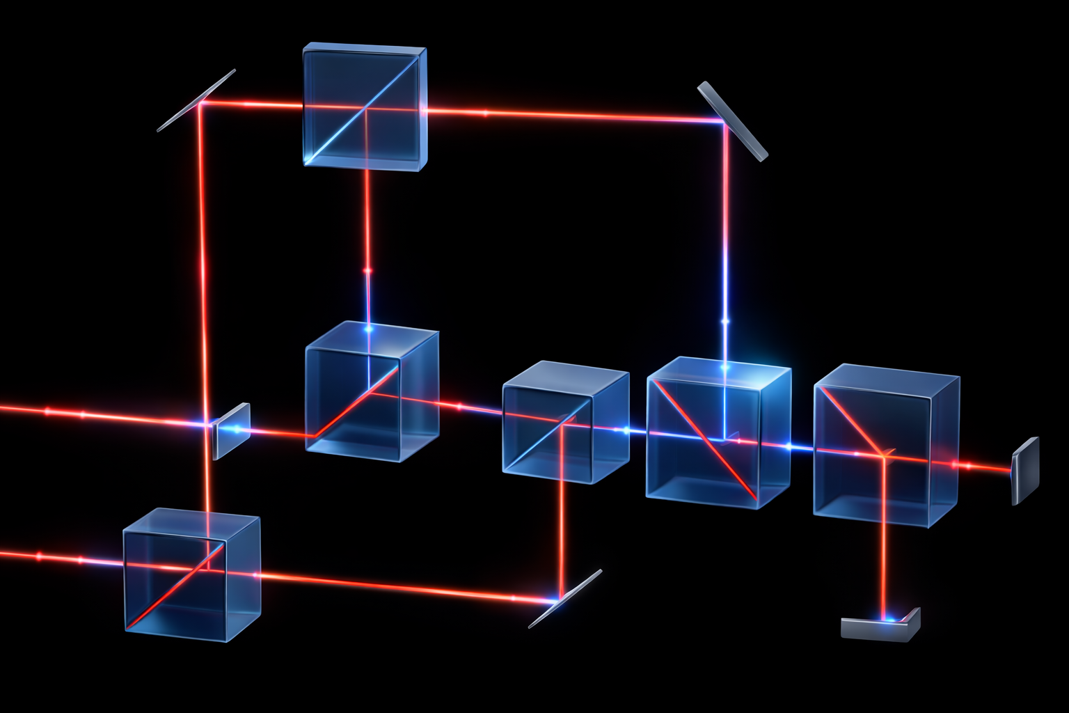
The object considered in this study is the metrology-oriented bulk-optics architecture of a stochastic optical AND gate shown in Figure 1.
Here, H≡1 and V≡0. The module is evaluated through the corrected H- and V-channel output intensities, IH and IV, and the ratio-based decision variable q=IH/(IH+IV).
The module operates with polarization encoding, where the horizontal polarization state is associated with the logical value 1 and the vertical polarization state is associated with the logical value 0. Two optical input streams, denoted Ak and Bk, are routed through a set of polarization-sensitive and non-polarizing bulk-optics elements, including asymmetric polarization beam splitters, beam splitters, mirrors, a polarization combiner, and a final polarization analyzer.
The architecture is intentionally interpreted as a functional module rather than as a collection of ideally symmetric branches. In particular, the early polarization routing stage may include a deliberately asymmetric split between the useful and auxiliary optical paths. Such asymmetry is not introduced as an imperfection, but as part of the functional design logic that helps maintain a robust distinction between the target output state HH and the non-target states HV, VH, and VV. In this sense, the module is not evaluated by branch equality, but by output correctness and by the available operational margin after all optical transformations and readout corrections have been taken into account.
At the output, the module is read by two photodetection channels associated with the horizontal and vertical components after the final polarization analysis stage. The decision variable is defined in ratio form as
where IH and IV are the corrected output intensities in the H and V detection channels, respectively. This readout form is physically convenient because it suppresses part of the sensitivity to common-mode changes of absolute intensity. However, it does not eliminate the need to control the absolute signal level. For that reason, the total corrected signal
is considered alongside the ratio response. The use of both q and S as complementary measurands is one of the key features of the proposed metrological treatment.
The module is verified using the four deterministic logical states HH, HV, VH, and VV, listed in Table 1 together with the corresponding decision rules. Under ideal AND behavior, the state HH must lead to H-dominant output and therefore to a large ratio value q, whereas the remaining three states must lead to V-dominant output and thus to low values of q. The practical verification problem is therefore not only to confirm the nominal truth-table behavior, but also to quantify how far the observed responses remain from the decision boundary under realistic non-idealities, drift, and measurement uncertainty.
This interpretation naturally leads to a two-level metrological strategy. The first level is basic verification, which is carried out directly at the module level through repeated measurements of the four logical states and application of the acceptance criteria. The second level is extended diagnostics, invoked only if the basic verification result is unsatisfactory or if the safety margin becomes too small. In that case, component-related parameters such as detector gains, dark offsets, leakage terms, or effective splitting ratios may be analyzed to identify the physical source of the deviation. Thus, component-level information supports diagnosis, but the decisive acceptance decision remains module-based.
3. Measurands, Measurement Conditions, and Power-Budget Model
3.1. Measurands and Decision-Oriented Quantities
The proposed methodology distinguishes between primary corrected output quantities, derived readout quantities, and decision-oriented figures of merit. The basic corrected output quantities are the H-channel and V-channel intensities, denoted IH and IV. From these, two derived measurands are formed: the ratio-based decision variable q and the corrected total signal S are defined by Eqs. (1) and (2), respectively.
The ratio q is responsible for functional discrimination between the target state HH and the non-target states HV, VH, and VV, while S is used to ensure that the module remains metrically observable and does not operate in an excessively weak-signal regime. The registry of the principal symbols, measurands, and model parameters used in the study is summarized in Table 2.
To transform these measurands into an acceptance decision, two scalar margins are introduced. The first one is the functional decision margin, denoted MΔ, which quantifies the minimum distance of the corrected ratio responses from the forbidden decision band around the threshold. The second one is the signal sufficiency margin, denoted MS, which quantifies the minimum distance of the corrected total signal from the admissible lower signal limit. In the uncertainty-aware version of the method, both margins are evaluated with expanded uncertainties included in the conformity rule. This treatment follows the general logic of uncertainty-based conformity assessment and guard-band decision rules [6,7,8].
3.2. Validity Conditions of the Verification Result
The result of calibration and verification is considered valid only under explicitly stated measurement conditions. In the present work, these conditions include the operating wavelength, ambient temperature and its admissible tolerance, warm-up time, normalized input optical power, detector linear range, and the defined acquisition window for repeated measurements. Such conditions are not secondary practical details; they determine the domain in which the measurement model and the associated conformity decision remain applicable.
This point is especially important for optical modules of the present type, because both the optical routing stage and the photodetection stage may exhibit sensitivity to alignment, source stability, and drift of effective channel gains or offsets. Therefore, the validity conditions are treated as an integral part of the verification statement. In other words, the decision that a module is operable is not understood as an unconditional claim, but as a claim valid within the stated metrological and operating envelope. This interpretation is consistent with internationally accepted metrological guidance for the specification of measurement procedures, validity of results, and competence-related requirements in calibration activity [6,7,8,9,10,11].
3.3. Optical Power-Budget Model
In order to support calibration and verification by physically interpretable parameters, the module is represented by a compact explicit optical power-budget model rather than by an abstract logic transfer function alone. Let the nominal input optical powers corresponding to the active logical input state be denoted by PA,in and PB,in, and let these be normalized for the model study. The optical transformation inside the module is then described through effective coefficients representing asymmetric polarization splitting, beam-splitter division, insertion losses, residual cross-leakage between polarization paths, and optical background terms.
The resulting optical intensities incident on the H and V detection channels are denoted by JH and JV. These quantities are absolute optical outputs of the module before detector gain, offset, resolution, and quantization effects are applied. In compact form, they may be written as
where s ∈ {HH, HV, VH, VV} denotes the tested logical state, are state-dependent optical contributions from individual internal paths, and are effective products of routing, splitting, and loss coefficients along those paths, and , are optical background terms.
This explicit power-budget representation is important for two reasons. First, it makes it possible to connect the functional behavior of the module to physically meaningful drift mechanisms such as increased leakage, redistribution of splitting ratios, or additional path losses. Second, it reveals that correct ratio behavior alone is insufficient for metrological acceptance: due to the cumulative effect of optical splitting and losses, the absolute output signal may become substantially lower than the normalized input level. Thus, a physically correct verification methodology has to monitor both discrimination quality and signal sufficiency.
3.4. Measurement Model and Transition to Corrected Outputs
The optical outputs JH and JV are transformed into measured detector signals through channel gains, dark offsets, random noise, bounded accuracy contributions, resolution effects, and quantization. After this, calibrated correction parameters are applied to obtain the corrected intensities IH and IV. Although the ratio variable q is less sensitive to some common-mode fluctuations than a single-channel decision metric, it remains sensitive to unequal drift between the two channels and to low-signal conditions in which offsets and quantization effects become relatively significant. For this reason, the present work does not treat q as a sufficient standalone criterion. Instead, it is paired with the total corrected signal S, forming a two-measurand basis for module-level acceptance.
In the next sections, this model is used to construct the calibration procedure, the basic verification procedure, and the rules for periodic re-verification of the module.
4. Measurement Model and Acceptance Criteria
4.1. Detector and Correction Model
The optical outputs of the module, JH and JV, are transformed into measured detector signals by the response of the H-channel and V-channel photodetection paths. In the present work, each channel is described by a compact measurement model that includes gain, dark offset, random noise, bounded instrumental accuracy, resolution, and quantization. For a given logical state s, the raw detector outputs may be written as
where and are the true gains of the detector channels, and are their dark offsets, and represent stochastic noise contributions, and represent bounded instrumental scale deviations, and , denote resolution and quantization operators. In addition, the detector outputs are constrained by the admissible linear operating range specified in the validity conditions. This formulation is sufficiently detailed to reflect the main metrologically relevant contributions while remaining compact enough for repeated simulation and verification studies [6,10,11].
The purpose of calibration is to estimate the correction parameters , , ,, which are then used to transform the measured detector outputs into corrected intensities:
After correction, negative values are physically non-interpretable for the present model and are therefore limited to zero. This step is not a logical transformation but a standard consistency condition for corrected optical intensities. The corrected outputs and are the primary quantities from which all further decision-oriented quantities are derived.
The role of the correction model is therefore twofold. First, it compensates for deterministic channel-to-channel differences that would otherwise bias the ratio readout. Second, it separates module behavior from measurement-channel behavior, which is essential for periodic re-verification and for distinguishing between physical degradation of the optical module and degradation of the readout system itself.
4.2. Ratio and Total-Signal Readout
The stochastic optical AND module is evaluated by two derived readout quantities. The first is the ratio-based decision variable q, defined in Eq. (1), which describes the dominance of the H-channel after correction. For the target state HH, correct module behavior requires q to be close to unity, whereas for the non-target states HV, VH, and VV, correct behavior requires low values of q.
The second quantity is the corrected total signal S, defined in Eq. (2). This quantity is introduced because ratio correctness alone does not guarantee metrological adequacy. In particular, if the total signal becomes too low, the influence of dark offsets, quantization, and channel-specific uncertainty may become disproportionately large even when the nominal ratio remains apparently correct. Therefore, the present approach treats q and S as complementary readout quantities rather than as alternatives.
This two-measurand structure is central to the proposed methodology. The ratio q captures the functional discrimination between the desired and undesired logical outputs, while the total signal S ensures that this discrimination remains physically supported by a sufficiently strong and metrically interpretable signal.
4.3. Functional Decision Criterion
To avoid ambiguous decisions near the threshold, the module is assessed using a threshold band with a forbidden decision zone rather than a single hard threshold. Let T be the central threshold and ΔT be the half-width of the forbidden band. Then the interval
is treated as a forbidden decision region. A module is functionally acceptable only if the corrected ratio responses remain outside this band in the appropriate direction for all four test states.
Accordingly, the basic acceptance inequalities are
To express this in scalar form, the functional decision margin is defined as
A positive value of indicates that the corrected ratio responses satisfy the functional acceptance rule with nonzero margin, whereas ≤0 indicates loss of functional operability.
The structure of the state-wise decision rules is summarized in Table 1. This table forms the operational core of the basic verification procedure and establishes the direct relation between the truth-table states and the metrological decision logic.
4.4. Signal Sufficiency Criterion
Functional correctness of the ratio readout does not guarantee that the module operates with sufficient signal strength. Due to asymmetric splitting, beam-splitter division, insertion losses, and detector limitations, the module may enter a regime in which the corrected total signal becomes too weak for reliable metrological interpretation. To address this, a lower admissible signal limit is introduced.
For each logical state, the corrected total signal must satisfy
In scalar form, the signal sufficiency margin is defined as
A positive value of indicates that the module remains above the minimum admissible corrected signal level in all verification states, while ≤0 indicates inadequate signal support for one or more states. This criterion is especially important in optical architectures where common-mode attenuation does not necessarily destroy ratio contrast immediately, but may still compromise the reliability of the verification result.
4.5. Uncertainty-Aware Conformity Decision
In accordance with uncertainty-based conformity assessment, the final acceptance decision is not taken from the nominal mean values alone. Instead, the state-wise uncertainties of q and S are propagated into the conformity rule by expanded uncertainties Uq and US. For the functional decision criterion, the uncertainty-aware margin is defined as
Similarly, for signal sufficiency,
The module is considered uncertainty-aware acceptable only if
This dual-criterion rule is consistent with the general logic of decision rules with guard bands and is intended to reduce the risk of incorrect conformity decisions [6,7,8]. In practice, the uncertainty-aware criteria are the decisive ones for final verification statements, while the mean-only criteria are retained as informative auxiliary indicators.
5. Calibration Procedure
5.1. Scope and Role of Calibration
The calibration procedure proposed in this work is intentionally limited to those quantities that are necessary to support correct readout of the module at the functional level. In the present methodology, calibration is focused on the detector channels and on the correction model rather than on full component-wise optical characterization of all bulk-optics elements. This choice follows directly from the metrological philosophy adopted here: component-level quantities are diagnostically useful, but routine acceptance of the module must be based on module-level output correctness.
Accordingly, the primary calibration outputs are the dark offsets and gains of the H and V detection channels. These parameters are later used to correct the measured outputs and to form the derived quantities q and S. The calibration result is therefore not an end in itself, but an enabling step for meaningful functional verification. This structure is compatible with measurement-management and calibration principles that distinguish between metrological support of the measuring chain and the final conformity decision regarding the functional object under test [10,11,13,14].
5.2. Dark-Offset Calibration
The first calibration step is the estimation of the dark offsets of the detector channels. This is performed in a dedicated zero-input acquisition mode in which the optical input to the considered detector channel is set to zero and the lower clipping behavior associated with ordinary working measurements is disabled. The purpose of this dedicated mode is to avoid artificial inflation of the dark estimate by the lower boundary of the normal linear operating range.
For each channel, a series of repeated measurements is recorded under dark conditions, and the mean value is used as the calibrated dark offset:
The standard deviation of the repeated measurements is used to estimate the associated uncertainty contribution. This approach is simple, physically interpretable, and directly connected to the additive baseline of the detector-electronics chain.
5.3. Gain Calibration
The second calibration step is the estimation of detector gains using a known optical reference level. For each detector channel, a repeated measurement series is acquired at a reference optical input Jref, and the gain is estimated after subtraction of the previously calibrated dark offset:
The gain uncertainty is evaluated from the repeated measurements of the reference series and, where appropriate, may be supplemented by the uncertainty of the reference optical level itself. In the present model study, the emphasis is placed on repeatability and detector-related uncertainty contributions, while the reference level is treated as known within the assumed simulation framework.
Taken together, dark-offset calibration and gain calibration define the working correction model of the measurement channels. These calibrated parameters are then used in all subsequent verification and re-verification procedures.
5.4. Calibration Outputs and Calibration Passport
The output of the calibration procedure is a compact calibration passport that contains the calibrated channel parameters together with their associated uncertainties and the comparison between estimated and nominal model values. A representative summary of such results is given in Table 3. In the present work, this table is intentionally kept compact in the main paper, while full repeated calibration datasets are provided in the supplementary material [12].
From the methodological point of view, the calibration passport has two functions. First, it documents the state of the readout channels at the moment of calibration. Second, it provides the parameter set required to interpret later verification results and to distinguish, during periodic re-verification, between detector-related drift and genuine optical-module degradation. At the same time, it is important to emphasize that satisfactory calibration of the readout channels does not automatically imply satisfactory module operation. The calibration procedure supports verification, but does not replace it.
6. Basic Verification Procedure and Acceptance Rules
6.1. General Verification Sequence
The proposed basic verification procedure is designed as the main routine conformity assessment of the module. It is intentionally compact and relies only on module-level measurements rather than on exhaustive component-level testing. The procedure consists of the following steps:
- ⁻
- establish the validity conditions of the measurement session;
- ⁻
- apply the calibrated correction model to the detector channels;
- ⁻
- sequentially generate the four verification states HH, HV, VH, and VV;
- ⁻
- acquire repeated measurements for each state;
- ⁻
- compute the corrected quantities IH, IV, q, and S;
- ⁻
- estimate state-wise uncertainties;
- ⁻
- evaluate the decision and signal-sufficiency margins;
- ⁻
- assign the final verification verdict.
This structure reflects the practical requirement that routine verification should remain feasible and cost-effective while still being metrologically justified. The state set and the associated acceptance rules are summarized in Table 1, while a representative calibration summary supporting the correction model is given in Table 3.
6.2. State-Wise Repeated Acquisition and Statistical Estimation
For each verification state, the detector outputs are recorded repeatedly in order to estimate the mean corrected response and its associated uncertainty. The repeated measurements serve two roles. First, they suppress the influence of accidental fluctuations on the final decision. Second, they provide the statistical basis for uncertainty evaluation of the state-wise quantities q and S.
For a state s, let the repeated corrected ratio and total-signal values be denoted and , where . The mean values are then
The corresponding standard uncertainties are estimated from the repeatability of the repeated measurement series, and expanded uncertainties are obtained using the selected coverage factor. In the present study, the results are reported in metrologically rounded form, so that the numerical resolution of reported values remains consistent with the associated uncertainty.
6.3. Acceptance Rules for Basic Verification
The module is accepted by the basic verification procedure only if both the functional decision criterion and the signal sufficiency criterion are satisfied. In the mean-only form, this requires
In the stricter uncertainty-aware form, the requirement becomes
The uncertainty-aware version is taken as decisive in the final conformity statement. In this way, a module is not accepted merely because the nominal mean responses are favorable; it must also retain sufficient margin after accounting for measurement uncertainty.
The use of the four deterministic states HH, HV, VH, and VV ensures that verification is directly linked to the truth-table behavior of the AND operation. At the same time, the dual-margin approach prevents a purely ratio-based but weakly supported output from being accepted as metrically adequate.
6.4. Practical Verdict Classes
In addition to the binary pass/fail outcome, the proposed methodology introduces a practical classification of module condition into four verdict classes:
- ⁻
- Pass: both uncertainty-aware margins are positive and comfortably above zero;
- ⁻
- Warning / reduced margin: the module remains formally acceptable, but one or both margins are small;
- ⁻
- Recalibration required: the mean-only rule is still favorable, but the uncertainty-aware rule is not;
- ⁻
- Reject: the module fails the acceptance criteria.
This classification is useful for practical maintenance and periodic control. In particular, it creates a natural link between routine verification and extended diagnostics. A module classified as Pass may continue operation under the defined validity conditions. A module classified as Warning / reduced margin may remain operational but requires closer monitoring or a shortened re-verification interval. A module classified as Recalibration required should not be rejected immediately; instead, recalibration of the readout channels or additional diagnostics should be performed first. Only when the acceptance criteria remain unsatisfied after such corrective action does the verdict Reject become appropriate.
Representative results of the basic verification and periodic re-verification procedures are summarized later in Figure 2 and Figure 3, and Table 4, where the evolution of corrected responses and margins under drifted conditions is examined.
The quantities qHH, qHV, qVH, and qVV denote the corrected ratio responses for the four verification states. The quantities SHH, SHV, SVH, and SVV denote the corresponding corrected total signals. The values MΔ,U and MS,U are the uncertainty-aware functional decision margin and signal sufficiency margin, respectively.
7. Model Case Study of Calibration and Periodic Re-Verification
7.1. Initial Calibration Results
The proposed methodology was first evaluated under nominal conditions by applying the calibration procedure described in Section 5. The resulting calibration passport is summarized in Table 3. In the model case considered here, the calibrated dark offsets and gains of the H and V detector channels were recovered with good agreement relative to their corresponding true model values. This confirms that the dedicated dark-calibration mode and the reference-level gain-calibration mode provide a consistent basis for the subsequent correction of detector outputs.
From the metrological perspective, this result is important for two reasons. First, it shows that the correction model can be identified without relying on the assumption of ideal detector symmetry. Second, it confirms that the detector-level calibration step remains compact and operationally feasible while still being sufficiently accurate for module-level conformity assessment. At the same time, the calibration result alone does not establish module operability; it only provides the corrected basis on which the verification decision can later be made.
In practical terms, the calibration passport should therefore be interpreted as a supporting document for verification rather than as a substitute for verification. This distinction is central to the present work: satisfactory estimation of does not imply satisfactory AND-gate performance unless the module also satisfies the state-wise decision and signal-sufficiency criteria.
7.2. Initial Verification Results
After calibration, the module was subjected to the basic verification procedure using the four deterministic logical states HH, HV, VH, and VV. The corrected ratio and total-signal responses obtained for the nominal case are included in the state-wise and scenario-wise verification outputs, while the compact scenario summary is reflected in Table 4 and graphically supported by Figure 2 and Figure 3.
Under nominal conditions, the corrected ratio response for the target state HH remained close to unity, whereas the responses for the non-target states HV, VH, and VV remained low and well separated from the forbidden decision band. At the same time, the total corrected signal in all states remained above the minimum admissible level Smin. Consequently, both the functional decision margin and the signal sufficiency margin remained positive, including their uncertainty-aware forms. This confirms that the module is not only logically correct under nominal conditions but also metrically supported by a sufficiently strong output signal.
The nominal verification case therefore illustrates the intended operation of the acceptance logic. The state HH produces an H-dominant output with a high corrected ratio, while the remaining three states produce V-dominant outputs with low corrected ratios. Because these outputs are simultaneously separated from the decision band and supported by sufficient total signal, the module is classified as acceptable without ambiguity. This establishes the nominal reference point for all subsequent re-verification scenarios.
7.3. Periodic Re-Verification Under Drift Scenarios
To evaluate the suitability of the proposed methodology for periodic control, the calibrated module was next examined under a set of drift scenarios representing gradual degradation of optical and detector-related parameters. These scenarios included increased polarization leakage, redistribution of asymmetric splitting ratios, additional path losses, detector gain drift, dark-offset drift, and combined aging effects. Their compact summary is given in Table 4, while the corresponding state-wise responses and margins are shown in Figure 2 and Figure 3.
The results demonstrate that the verification framework remains physically interpretable under drift. In particular, increased leakage and redistribution of the splitting ratios tend to increase the corrected ratio of non-target states, thereby reducing the functional decision margin. At the same time, additional optical losses reduce the total corrected signal and thus reduce the signal-sufficiency margin. Detector-related drift affects both the corrected ratio and the corrected total signal through unequal channel correction errors, especially when the calibration passport is no longer fully representative of the current detector state.
An important observation is that the two margins respond differently to different degradation mechanisms. Some drift scenarios primarily reduce the functional separation between target and non-target states, while others predominantly reduce the available signal level. This confirms the usefulness of retaining both MΔ and MS in the verification methodology. A ratio-only interpretation would not be able to distinguish between a physically robust state with good signal support and a weak-signal state that still happens to preserve favorable ratio contrast.
The model case therefore supports the concept of periodic re-verification. Even when the module remains acceptable after moderate degradation, the reduction of margins provides a quantitative basis for tracking health state and for deciding whether the current operating condition is comfortably acceptable or approaching a warning region. In this way, periodic re-verification serves not only as a pass/fail checkpoint but also as a monitoring tool for operational margin.
7.4. Worked Lifecycle Example
A worked lifecycle example was further constructed to demonstrate how the proposed methodology can connect initial calibration, routine operation, drift, re-verification, and corrective action within a single coherent framework. The corresponding evolution of corrected ratio and total-signal responses is illustrated in Figure 4.
The lifecycle sequence begins with the initial calibrated state, proceeds through a moderate optical-drift stage, then through a detector-drift stage, and finally to a recalibrated detector state. The purpose of this sequence is not merely to provide another graphical summary, but to show that calibration and periodic re-verification can be naturally organized as repeated metrological actions over the service life of the module. In this sense, the module is not treated as a static object that is verified once and then assumed to remain stable indefinitely. Instead, its metrological state is considered dynamic and potentially subject to both optical and electronic drift.
The worked case also illustrates the intended relation between routine verification and corrective action. When the module remains comfortably within the admissible region, no intervention is required. When margins decrease or detector-related drift becomes significant, recalibration becomes a rational and targeted corrective measure. If recalibration is insufficient to restore the required margins, the methodology naturally escalates toward extended diagnostics or rejection. Thus, the lifecycle example shows that the proposed framework is not limited to a single inspection event, but can support an operational maintenance strategy over time.
8. Discussion
8.1. Why Module-Level Verification Is Decisive
The central methodological conclusion of this study is that acceptance of the stochastic optical AND gate should be based primarily on module-level functional verification, not on isolated component symmetry. This is a direct consequence of the physics of the considered architecture. The module contains intentional asymmetry in its optical routing stage, and this asymmetry can contribute positively to correct discrimination between the target state HH and the non-target states HV, VH, and VV. Therefore, the presence of unequal branches is not, by itself, evidence of a defect.
For this reason, the decisive acceptance question is not whether all intermediate optical paths are identical, but whether the final corrected outputs produce the correct decision with sufficient margin and sufficient signal support. This observation is particularly important for practical metrology, because it avoids over-constraining the verification procedure with unnecessary component-level criteria that may increase cost without increasing relevance to actual module performance.
8.2. Basic Verification Versus Extended Diagnostics
A second important conclusion is that the verification methodology should remain layered. The basic verification procedure is sufficient for routine conformity assessment because it directly addresses the functional task of the module. It is compact, state-based, and operationally economical. In contrast, extended diagnostics should not be mandatory for every routine verification cycle. Their role is to support root-cause analysis when the basic verification result is unsatisfactory or when the margins become too small.
This distinction is essential for practical deployment. If every verification cycle required full component-level investigation, the procedure would become unnecessarily expensive and would lose its attractiveness as a metrological routine. By contrast, the present framework preserves a clear hierarchy: basic verification provides the acceptance decision, while extended diagnostics provide deeper interpretation only when needed. This makes the method both scientifically sound and practically realistic.
8.3. Interpretation of the Dual-Margin Approach
The introduction of two acceptance margins, MΔ and MS, is one of the key conceptual features of the proposed methodology. The first margin addresses the logical discrimination capability of the module, while the second addresses the adequacy of the supporting signal level. The model results show that these two aspects are not redundant. Different drift mechanisms may reduce them in different ways, and therefore both are needed to represent the operational health of the module.
This dual-margin interpretation is especially relevant in optical architectures where attenuation may accumulate over several bulk-optics stages. Under such conditions, the ratio variable may remain favorable longer than the absolute signal level. If only the ratio is monitored, a weak-signal regime may be incorrectly accepted as operationally safe. Conversely, if only the signal level is monitored, the module may appear healthy despite losing functional discrimination. The simultaneous use of MΔ and MS avoids both types of misinterpretation.
8.4. Role of Boundary Analysis
The boundary analysis developed in this work should be interpreted as a methodological and design-oriented layer, not as a compulsory part of every routine verification cycle. Its main value lies in three areas: first, it helps identify the most influential degradation mechanisms; second, it helps interpret reduced-margin states observed during re-verification; third, it supports the rationale for selecting re-verification intervals and warning thresholds.
In the present study, the boundary analysis also reveals a practical limitation: if the explored parameter ranges remain entirely within the pass region, the resulting admissible limits must be interpreted only as lower bounds on the true operability boundary. This observation is methodologically useful because it prevents over-interpretation of incomplete sweep ranges. In future refinement of the model or in an experimental realization, wider or adaptively refined parameter sweeps would be desirable to obtain sharper quantitative operability limits.
8.5. Practical Metrological Implications
From a practical perspective, the proposed approach offers a useful compromise between rigor and cost. It retains explicit measurement conditions, calibrated correction of detector outputs, uncertainty-aware conformity assessment, and physically interpretable drift analysis, while keeping the routine verification sequence compact. This is particularly relevant in contexts where the transition toward European-aligned metrological practices requires that uncertainty, conformity rules, traceability-related thinking, and documented validity conditions be incorporated into emerging photonic measurement methodologies [6,7,8,9,10,11,13,15].
At the same time, the present work should be understood as a model-based methodological study rather than a complete industrial verification standard. Further work may include experimentally derived component distributions, correlation between channel uncertainties, tighter modeling of detector nonlinearity, and experimentally justified re-verification intervals. Nevertheless, the current framework already provides a coherent structure that can be directly used to organize calibration, basic verification, and corrective maintenance logic for this class of optical stochastic modules.
9. Conclusions
A metrological framework for calibration, verification, and periodic re-verification of a metrology-oriented bulk-optics stochastic optical AND gate with ratio-based polarization readout has been proposed. In contrast to approaches that focus primarily on nominal component symmetry, the present methodology treats the module as a functional measurement object whose acceptability is determined by corrected output behavior under specified operating conditions.
The proposed framework is based on explicitly defined measurands, validity conditions, a compact optical power-budget model, a detector correction model, and an uncertainty-aware conformity rule. Two complementary decision metrics were introduced: the functional decision margin MΔ, which quantifies separation from the forbidden decision band, and the signal sufficiency margin MS, which ensures that the corrected output remains metrically reliable. Their uncertainty-aware forms, MΔ,U and MS,U, were used as the decisive criteria in conformity assessment.
A practical calibration procedure was formulated for detector dark offsets and gains, and a compact basic verification procedure was established using the four deterministic logical states HH, HV, VH, and VV. The model case study demonstrated that the proposed framework can support both initial acceptance and periodic re-verification under drift. The results also showed that monitoring ratio responses alone is insufficient for a robust metrological interpretation, and that signal sufficiency must be assessed alongside decision correctness.
An important practical conclusion is that routine verification should remain module-based and compact, whereas extended diagnostics and operability-boundary analysis should serve as deeper support layers rather than as obligatory parts of every verification cycle. In this way, the proposed methodology provides a balanced structure that is both metrologically justified and operationally feasible. Owing to its uncertainty-aware and standards-compatible logic, the framework is well suited for further refinement toward experimental implementation and for adaptation to European-aligned metrological practice in photonic measurement systems [6,7,8,9,10,11,13,15].
Supplementary Materials
The following supporting information can be downloaded at the website of this paper posted on Preprints.org, or in the Figshare repository [12].
Author Contributions
The author solely conceived the study, developed the methodology, performed the modeling, analyzed the results, prepared the figures and tables, and wrote the manuscript.
Funding
This research received no external funding.
Institutional Review Board Statement
This study did not involve human participants, human data, or animal subjects, and therefore did not require ethical approval.
Data Availability Statement
All data and code are available in the Figshare supplementary repository [12]. The package includes the Colab notebooks used for simulation, exported datasets (CSV/JSON), and configuration manifests enabling full reproducibility of the reported results. No external datasets were used in this study.
Conflicts of Interest
The author declares no conflict of interest.
Reproducibility Statement
All numerical results reported in this study can be reproduced using the provided Colab notebooks and configuration files included in the Supplementary Materials [12]. The workflows use fixed random seeds and documented parameter settings, ensuring that the figures and tables can be regenerated from the distributed datasets and scripts.
References
- Gaines BR. Stochastic computing systems. Advances in Information Systems Science. 1969; 2:37–172.
- Alaghi A, Hayes JP. Survey of stochastic computing. ACM Transactions on Embedded Computing Systems. 2013;12(2s): Article 92, 1–19. [CrossRef]
- Bhardwaj A, Hedekvist PO, Vahala K. All-optical logic circuits based on polarization properties of nondegenerate four-wave mixing. Journal of the Optical Society of America B. 2001;18(5):657–665. [CrossRef]
- Guo LQ, Connelly MJ. All-optical AND gate with improved extinction ratio using signal induced nonlinearities in a bulk semiconductor optical amplifier. Optics Express. 2006;14(7): 2938–2943. [CrossRef]
- Liu Y, Chen L, Xu T, Mao J, Zhang S, Liu Y. All-optical signal processing based on semiconductor optical amplifiers. Frontiers of Optoelectronics. 2011; 4(3): 231–242. [CrossRef]
- JCGM 100:2008. Evaluation of measurement data—Guide to the expression of uncertainty in measurement. Joint Committee for Guides in Metrology; 2008. [CrossRef]
- JCGM 106:2012. Evaluation of measurement data—The role of measurement uncertainty in conformity assessment. Joint Committee for Guides in Metrology; 2012. [CrossRef]
- JCGM 200:2012. International vocabulary of metrology—Basic and general concepts and associated terms (VIM). 3rd ed. Joint Committee for Guides in Metrology; 2012. [CrossRef]
- ISO/IEC 17025:2017. General requirements for the competence of testing and calibration laboratories. Geneva: International Organization for Standardization; 2017.
- EA-4/02 M: 2022. Evaluation of the Uncertainty of Measurement in Calibration. European co-operation for Accreditation; 2022.
- ILAC G8:09/2019. Guidelines on Decision Rules and Statements of Conformity. International Laboratory Accreditation Cooperation; 2019.
- Strynadko M. Supplementary materials for “Metrological verification and calibration of a bulk-optics stochastic optical AND gate with ratio-based polarization readout”. figshare. 2026. [CrossRef]
- ILAC G24:2022. Guidelines for the Determination of Recalibration Intervals of Measuring Equipment. International Laboratory Accreditation Cooperation; 2022.
- ISO 10012:2026. Quality management—Requirements for measurement management systems. Geneva: International Organization for Standardization; 2026.
- ILAC P10:07/2020. ILAC Policy on Metrological Traceability of Measurement Results. International Laboratory Accreditation Cooperation; 2021.
Figure 1.
Metrology-oriented bulk-optics architecture of the stochastic optical AND gate with ratio-based polarization decision readout.
Figure 1.
Metrology-oriented bulk-optics architecture of the stochastic optical AND gate with ratio-based polarization decision readout.

Figure 2.
State-wise corrected ratio response q and corrected total signal S under nominal and drifted conditions for the stochastic optical AND module. The upper panel shows the evolution of the ratio-based decision variable for the four verification states HH, HV, VH, and VV, together with the central threshold and the forbidden decision band. The lower panel shows the corresponding corrected total signal and the minimum admissible signal level Smin.

Figure 3.
Functional decision margin and signal sufficiency margin versus degradation level for the stochastic optical AND module. The upper panel shows the mean-only and uncertainty-aware functional margins, MΔ and MΔ,U, while the lower panel shows the corresponding signal margins, MS and MS,U. The zero line denotes the operability limit.

Figure 4.
Worked model case of calibration and periodic re-verification of the stochastic optical AND module. The upper panel shows the evolution of the corrected ratio response q, and the lower panel shows the evolution of the corrected total signal S, for the four verification states HH, HV, VH, and VV across the considered lifecycle stages. The threshold band and the minimum admissible signal level Smin are indicated for reference.


Table 1.
Verification states, ratio-based acceptance rules, and signal-sufficiency criteria for the basic verification procedure of the stochastic optical AND module. The table defines the required decision side for each state and summarizes the mean-only and uncertainty-aware conformity conditions.
| Verifica-tion state | Expected logic output | Required decision side | Mean-only ratio condition | Uncertainty-aware ratio condition | Mean-only signal condition | Uncertainty-aware signal condition |
| HH | 1 | Above upper band edge | qHH > T +ΔT | qHH -Uq(HH) > T+ΔT | SHH > Smin | SHH - US(HH) > Smin |
| HV | 0 | Below lower band edge | qHV < T - ΔT | qHV + Uq(HV) < T - ΔT | SHV > Smin | SHV - US(HV) > Smin |
| VH | 0 | Below lower band edge | qVH < T - ΔT | qVH + Uq(VH) < T - ΔT | SVH > Smin | SVH - US(VH) > Smin |
| VV | 0 | Below lower band edge | qVV < T - ΔT | qVV + Uq(VV) < T - ΔT | SVV > Smin | SVV - US(VV) > Smin |
Note. Here, q=IH/(IH+IV) is the corrected ratio-based decision variable, S=IH+IV is the corrected total signal, T is the central decision threshold, ΔT is the half-width of the forbidden decision band, and Uq and US are the expanded uncertainties of q and S, respectively.
Table 2.
Symbol, measurand, and key parameter registry used in the measurement model of the metrology-oriented stochastic optical AND module. The table includes the primary corrected intensities, derived readout quantities, decision metrics, and the principal optical, detector, and decision-rule parameters used in the main-text analysis.
| Category | Symbol / parameter | Meaning | Role in the model | Nominal value |
|---|---|---|---|---|
| Measurand | IH | Corrected H-channel intensity | Primary corrected output | — |
| Measurand | IV | Corrected V-channel intensity | Primary corrected output | — |
| Derived quantity | q = IH/(IH + IV) | Ratio-based decision variable | Functional discrimination | — |
| Derived quantity | S = IH + IV | Corrected total signal | Signal sufficiency assessment | — |
| Decision metric | MΔ | Functional decision margin | Acceptance criterion | — |
| Decision metric | MS | Signal sufficiency margin | Acceptance criterion | — |
| Decision setting | T | Central decision threshold | Ratio-based conformity rule | 0.50 |
| Decision setting | ΔT | Half-width of forbidden decision band | Ratio-based conformity rule | 0.10 |
| Decision setting | Smin | Minimum admissible corrected total signal | Signal sufficiency rule | 0.08 |
| Optical parameter | H-directed fraction at PBS1 | Power-budget model | 0.80 | |
| Optical parameter | V-directed fraction at PBS1 | Power-budget model | 0.20 | |
| Optical parameter | H-directed fraction at PBS2 | Power-budget model | 0.80 | |
| Optical parameter | V-directed fraction at PBS2 | Power-budget model | 0.20 | |
| Optical parameter | Residual leakage from V path into H channel | Power-budget model | 0.015 | |
| Optical parameter | Residual leakage from H path into V channel | Power-budget model | 0.015 | |
| Optical parameter | Optical background in H channel | Power-budget model | 0.002 | |
| Optical parameter | Optical background in V channel | Power-budget model | 0.002 | |
| Detector parameter | True gain of H-channel detector | Detector model | 1.000 | |
| Detector parameter | True gain of V-channel detector | Detector model | 0.985 | |
| Detector parameter | True dark offset of H-channel detector | Detector model | 0.0020 | |
| Detector parameter | True dark offset of V-channel detector | Detector model | 0.0025 | |
| Instrument parameter | Resolution step of H-channel acquisition | Measurement model | 0.001 | |
| Instrument parameter | Resolution step of V-channel acquisition | Measurement model | 0.001 | |
| Instrument parameter | Bounded accuracy fraction of H-channel acquisition | Measurement model | 0.020 | |
| Instrument parameter | Bounded accuracy fraction of V-channel acquisition | Measurement model | 0.020 |
Note. The table lists only the compact subset of symbols and parameters used directly in the main-text discussion. The extended parameter registry, including additional optical, detector, and auxiliary simulation parameters, is provided in the Supplementary Package [15].
Table 3.
Initial calibration results for the detector-channel correction model. The table summarizes the calibrated dark offsets and gains of the H and V channels, together with their associated uncertainties and deviations from the corresponding nominal model values.
Table 3.
Initial calibration results for the detector-channel correction model. The table summarizes the calibrated dark offsets and gains of the H and V channels, together with their associated uncertainties and deviations from the corresponding nominal model values.
| Calibrated parameter | Meaning | Nominal / true model value | Estimated value | Expanded uncertainty | Absolute deviation | Reported form |
| Calibrated dark offset of H-channel detector | 0.0020 | 0.002033 | 0.000184 | 0.000033 | 0.00203 ± 0.00018 | |
| Calibrated dark offset of V-channel detector | 0.0025 | 0.002517 | 0.000154 | 0.000017 | 0.00252 ± 0.00015 | |
| Calibrated gain of H-channel detector | 1.0000 | 1.017528 | 0.002652 | 0.017528 | 1.0175 ± 0.0027 | |
| Calibrated gain of V-channel detector | 0.9850 | 0.976944 | 0.002311 | -0.008056 | 0.9769 ± 0.0023 |
Note. The dark-offset estimates were obtained in the dedicated dark-calibration mode, whereas the gain estimates were obtained from repeated measurements at a known optical reference level after subtraction of the corresponding calibrated dark offsets. Full repeated calibration datasets are provided in the Supplementary Package [12].
Table 4.
Drift scenarios and operability outcomes for periodic re-verification of the stochastic optical AND module. For each scenario, the table summarizes the corrected ratio responses, corrected total signals, decision and signal margins, and the resulting module verdict.
Table 4.
Drift scenarios and operability outcomes for periodic re-verification of the stochastic optical AND module. For each scenario, the table summarizes the corrected ratio responses, corrected total signals, decision and signal margins, and the resulting module verdict.
| Scenario | qHH | qHV | qVH | qVV | SHH | SHV | SVH | SVV | MΔ,U | MS,U | Verdict |
|---|---|---|---|---|---|---|---|---|---|---|---|
| S0 | 0.9898 | 0.0664 | 0.0664 | 0.0675 | 0.7545 | 0.2021 | 0.2020 | 0.2016 | 0.3314 | 0.1208 | Pass |
| S1 | 0.9899 | 0.1201 | 0.1199 | 0.1195 | 0.7621 | 0.2100 | 0.2093 | 0.2093 | 0.2790 | 0.1285 | Pass |
| S2 | 0.9890 | 0.0501 | 0.0509 | 0.0499 | 0.6967 | 0.2502 | 0.2507 | 0.2498 | 0.3484 | 0.1688 | Pass |
| S3 | 0.9892 | 0.0772 | 0.0772 | 0.0770 | 0.7139 | 0.2062 | 0.2072 | 0.2074 | 0.3217 | 0.1252 | Pass |
| S4 | 0.9832 | 0.1011 | 0.1020 | 0.1020 | 0.6270 | 0.3090 | 0.3084 | 0.3079 | 0.2970 | 0.2270 | Pass |
Note. S0 — reference condition after initial calibration; S1 — moderate growth of residual cross-leakage; S2 — asymmetric splitting drift and extra beam-path loss; S3 — detector gain and dark-offset drift; S4 — combined optical and detector degradation.
Disclaimer/Publisher’s Note: The statements, opinions and data contained in all publications are solely those of the individual author(s) and contributor(s) and not of MDPI and/or the editor(s). MDPI and/or the editor(s) disclaim responsibility for any injury to people or property resulting from any ideas, methods, instructions or products referred to in the content. |
© 2026 by the authors. Licensee MDPI, Basel, Switzerland. This article is an open access article distributed under the terms and conditions of the Creative Commons Attribution (CC BY) license (http://creativecommons.org/licenses/by/4.0/).
Copyright: This open access article is published under a Creative Commons CC BY 4.0 license, which permit the free download, distribution, and reuse, provided that the author and preprint are cited in any reuse.


