Submitted:
15 April 2026
Posted:
15 April 2026
You are already at the latest version
Abstract
Accurate delineation of buried slip surfaces remains a major uncertainty in landslide hazard assessment, especially where subsurface data are limited. This study evaluates a displacement-based approach to estimate quasi-three-dimensional (quasi-3D) slip surfaces using ground-surface displacement vector gradients derived from multi-temporal UAV-based LiDAR data. Two landslides in Japan (Jimba and Kamitokitozawa), representing contrasting scales, were analyzed to assess the method’s applicability and limitations. Two-dimensional (2D) slip-surface profiles were derived through group-wise median grouping of displacement gradients and weighted non-uniform rational B-spline fitting along longitudinal sections. Transverse profiles were constrained using side-scarp gradients and depths estimated from longitudinal profiles. These profiles were integrated into quasi-3D surfaces and validated against borehole-derived slip surfaces. At the Jimba landslide, characterized by relatively coherent movement, the estimated surfaces closely match borehole data in both depth and geometry. At the larger Kamitokitozawa landslide, the method reproduces first-order geometry and extent but shows larger local deviations, particularly in a graben-like subsidence zone. Nevertheless, the estimated displaced volume reaches 96% of that derived from borehole data. These results demonstrate that the method provides useful first-order constraints on slip-surface geometry for preliminary hazard assessment, borehole planning, and 3D stability analysis.
Keywords:
landslide slip surface
; UAV LiDAR
; surface displacement vector gradient
; quasi-3D modeling
; borehole data
; landslide hazard assessment
1. Introduction
Accurate characterization of landslide slip surfaces is fundamental to hazard assessment and mitigation. The geometry of a slip surface, including its depth, shape, orientation, and spatial extent, directly controls slope stability and landslide kinematics [1,2]. Reliable delineation of slip surfaces enables the estimation of critical parameters, including shear strength distribution [3] and the volume of mobilized material [1,4]. Moreover, slip-surface geometry is a primary input for limit equilibrium and numerical analyses [5], as well as for the design of stabilization measures. Uncertainty in slip-surface delineation, therefore, translates directly into the reduced reliability of hazard evaluations, risk assessments, and countermeasure planning.
A variety of direct and indirect methods have been developed to identify slip surfaces, each with distinct advantages and limitations. Direct approaches, including exploratory drilling and borehole logging, provide high-depth-resolution point data on subsurface stratigraphy and shear zones [6,7,8], but are spatially limited and costly when dense coverage is required. Indirect approaches, including geophysical methods such as electrical resistivity tomography (ERT) and ground-penetrating radar (GPR), infer slip surfaces from contrasts in physical properties [6]. Although these techniques can provide continuous spatial information, their accuracy depends strongly on survey layout, resolution, and site conditions, and prolonged surveys can impose substantial economic and logistical burdens.
An alternative line of research exploits ground-surface displacement patterns to infer buried slip surfaces based on kinematic principles. Assuming rigid-body motion, Carter and Bentley (1985) proposed a method for identifying circular slip surfaces in two-dimensional (2D) cross-sections using surface displacement vectors measured by total stations. This concept was later extended by Yoshizawa and Hosokawa [9] and Yoshizawa [10], who developed several approaches to estimate slip surfaces from the spatial distribution of ground-surface displacement vectors. However, these early studies relied on sparsely distributed measurements, which limited their robustness (e.g., [11]). To mitigate the errors associated with sparse displacement data, subsequent methods introduced weighting schemes and segmentation strategies along 2D profiles, such as the polygon method [12]. Nevertheless, the cumulative integration of displacement vector gradients from the landslide head often amplified noise unrelated to actual deformation, leading to inaccuracies in toe position estimation. To address this issue, non-uniform rational B-spline (NURBS) curves with appropriate weighting were introduced to smooth slip-surface geometries and suppress spurious fluctuations (e.g., [8]).
Yoshizawa [13] and Miyazawa et al. [14] extended this work and developed three-dimensional (3D) slip-surface reconstructions using higher-density displacement observations. These approaches include grouping surface displacement vectors with similar horizontal orientations and averaging their gradients [15] and constructing polyhedral slip surfaces composed of triangular facets [14]. Although effective, these methods require dense, continuous monitoring networks that are rarely available in practice, particularly at large landslides where instrument installation and long-term data acquisition are time-consuming and costly.
Recent advances in remote sensing, including UAV-based photogrammetry, UAV LiDAR, and InSAR, have enabled high-resolution and high-frequency measurement of ground-surface deformation, creating new opportunities for displacement-based slip-surface estimation [8,16,17]. In parallel, inverse modeling and numerical back-analysis techniques, often integrated with multi-temporal monitoring data (e.g., extensometers, inclinometers, GNSS), have been used to capture the deformation along the inferred slip surface (e.g., Dai et al., 2025). Building on these developments, Ogita et al. [8] proposed a displacement-based method for estimating 2D slip-surface geometry using high-density ground-surface displacement vectors derived from multi-temporal UAV LiDAR data for landslides in northeastern Japan. Their approach relies solely on topographic data and achieved agreement rates of 79%–90% with borehole-derived slip depths; however, the method was applied primarily along a single main survey line at each site, and its applicability to adjacent and transverse profiles remains unclear. In addition, the grouping of displacement vector gradients relied largely on visual interpretation, introducing subjectivity into the estimation process.
We extend the method of Ogita et al. [8] to two landslides of contrasting scale: the small- to medium-sized Jimba landslide and the large-sized Kamitokitozawa landslide in Japan (Figure 1). Using multi-temporal, high-density UAV LiDAR data, we introduce an objective procedure for grouping ground-surface displacement vector gradients based on group-wise median statistics. We apply the method to both longitudinal and transverse survey profiles, enabling the integration of multiple 2D slip-surface estimates into a quasi-3D slip surface using weighted smoothing techniques. We evaluate the performance and limitations of the proposed approach through systematic comparison with borehole-derived slip-surface data.
2. Geomorphological and Geological Setting of the Study Areas
2.1. Jimba Landslide
The Jimba landslide is located in an area underlain by Miocene basaltic lava [18]. The landslide, ~80 m wide and 120 m long, was active between April 2021 and August 2022 [19]. A graben-like subsidence zone formed immediately downslope of the main scarp, characterized by a depressed block that is ~45 m wide and 14 m long with a vertical displacement of <2 m (Figure 2 and Figure 3a). Step-like surface cracks are observed locally in the subsidence zone.
The slip surface was inferred from core logging and pipe strain-gauge observations obtained from six vertical boreholes and two horizontal boreholes (Figure 2), during 2021 and 2024 [19]. Figure 3(b) shows the strain records from borehole BV22-3, located near the center of the landslide. Following heavy rainfall in early August 2022 (216 mm between 1 and 3 August [20]), cumulative strain at a depth of ~15 m increased rapidly and subsequently exceeded the measurement range. Consistent with this observation, a clay-rich layer with well-developed slickensides was identified at a depth of 14.7 m in the corresponding borehole core and was interpreted as the slip surface (Figure 3c). Using the same criteria, slip-surface depths were estimated consistently in the remaining five boreholes. Additional support for a coherent slip surface was provided by rupture depths observed in horizontal drainage installations that were damaged by landslide movement. The locations of these rupture points were used as supplementary constraints in constructing contour lines for the inferred slip surface. The consistency between borehole, strain gauge, and drainage damage evidence indicates that landslide movement was dominated by sliding along a single, laterally continuous slip surface, with limited internal deformation.
UAV-based LiDAR surveys were conducted in April 2021 and August 2022, representing the pre- and post-event conditions, respectively. These surveys yielded a high-density point cloud with a mean density of >60 points/m2 (Table 1). During the 16 months between the two surveys, a ground extensometer installed at the landslide head (Figure 2) recorded a cumulative displacement of ~0.7 m. GNSS observations reported by Ogita et al. [8] further support this interpretation, showing consistent displacement directions across monitoring points within the landslide area.
2.2. Kamitokitozawa Landslide
The Kamitokitozawa landslide developed in a geologically heterogeneous setting composed of late Miocene to early Pliocene dacitic to rhyolitic volcanoclastic rocks interbedded with siltstone, sandstone, and conglomerate [18]. The landslide is ~650 m wide and 600 m long, covering a much larger area than the Jimba landslide. The landslide has a pronounced graben-like subsidence zone that is ~580 m wide and 260 m long, immediately downslope of the main scarp, with a vertical displacement of <8 m (Figure 4). The subsidence zone appears to have subsided as a coherent mass with few surface cracks.
A total of 41 boreholes were drilled in the landslide (Figure 4). The deepest slip surface was identified at a depth of 179.7 m in borehole BV22-24 (in the subsidence zone), based on the occurrence of a slickensided surface with well-developed striations (Figure 4 and Figure 5a, and b). Consistent with this interpretation, pipe strain-gauges installed at depths of 179 m and 180 m in September 2023 recorded progressive strain immediately after installation (Figure 5c), indicating ongoing displacement at this depth [21].
Landslide movement was first recognized in July 2018. UAV-based LiDAR surveys conducted in April 2020 and May 2022 yielded point clouds with average densities of ~30 and 160 points/m2, respectively (Table 1). During the 25 months between the two surveys, GNSS4 measurements at the landslide head (Figure 4) recorded cumulative ground displacements of up to ~6 m, indicating substantial and sustained movement of the landslide mass [21]. In addition, displacement directions recorded at multiple GNSS stations were not uniform, further reflecting complex kinematic behavior across the landslide [21].
3. Quasi-3D Slip Surface Estimation
3.1. Calculation of the Ground-Surface Displacement Vector Gradient
The ground-surface displacement vector gradients were derived by combining horizontal displacement vectors with vertical displacement components to represent the overall deformation of the landslide surface. Horizontal ground-surface displacement vectors were calculated using the sum of absolute difference (SAD) template matching technique (Figure 6a; e.g., [22]) by comparing shaded relief maps derived from digital elevation models (DEMs) obtained from the UAV-based LiDAR survey (Table 1). The calculations followed the method of Mukoyama (2011). The displacement analysis was validated by comparing independent GNSS displacement observations with ground-surface displacement vectors extracted from 2 m × 2 m meshes around the GNSS station. Vertical displacement was computed from the elevation differences between the pre- and post-movement coordinates associated with each horizontal displacement vector.
We used a DEM mesh size of 20 cm for the Jimba landslide and 50 cm for the Kamitokitozawa landslide. We adopted a finer mesh size for the Jimba landslide because its total displacement was ~60 cm (Section 2.1), which requires higher spatial resolution to accurately capture subtle topographic changes associated with small-scale movement. In contrast, the Kamitokitozawa landslide exhibited a larger displacement (<6 m; Section 2.2), for which a coarser 50 cm mesh size was sufficient to represent the deformation. Ogita et al. [8] demonstrated that using a mesh size smaller than the displacement has little effect on the accuracy of the estimated slip surface.
3.2. Grouping of the Ground-Surface Displacement Vector Gradients Along the Longitudinal Profiles
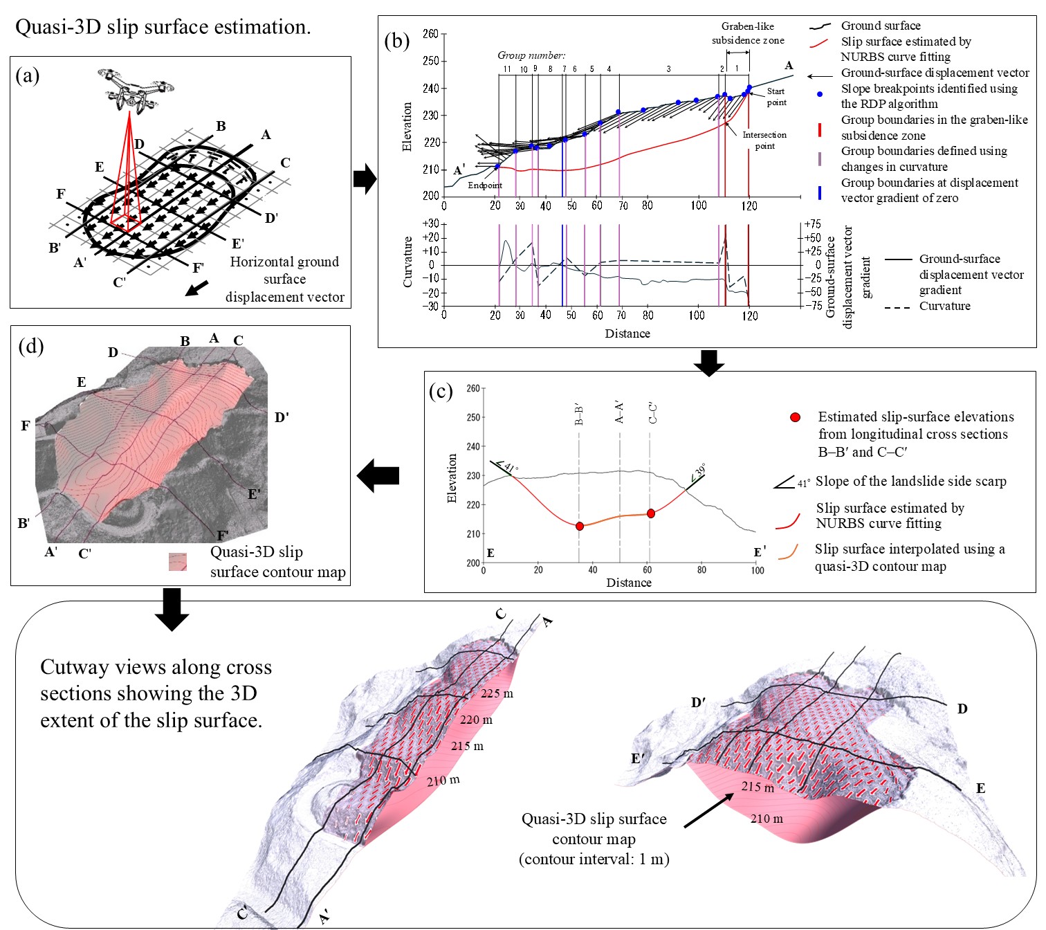
2D slip surfaces along the main (A–A′) and auxiliary (B–B′ and C–C′) cross-sections were inferred from longitudinal profiles of the ground-surface displacement vector gradient and curvature (Figure 6b), assuming that the inclination of the slip surface is consistent with the ground-surface displacement vector gradient (e.g., [23]). The estimation procedure was identical for all lines; therefore, we present the procedure for the A–A′ cross-section as a representative example. Inflection points in the ground-surface displacement vector gradients are commonly associated with convex or concave breaks along the longitudinal profile for the period after the landslide. To prevent overinterpretation of inflection points arising from small-scale topographic undulations captured in the high-resolution data, the post-landslide longitudinal profiles were first smoothed using the Ramer–Douglas–Peucker (RDP) algorithm applied to LiDAR point cloud data [24], with a tolerance threshold of 0.5 for the Jimba landslide and 2.5 for the Kamitokitozawa landslide. Ground-surface displacement vector gradients and curvatures were then projected along the longitudinal profiles, where the curvature was calculated from the smoothed profile as the inverse of the radius of a circular arc defined by three consecutive points. Finally, the ground-surface displacement vector gradients were grouped based on the combined interpretation of the displacement vector gradient and curvature profiles, with group boundaries defined at locations where the displacement vector gradient is zero (Figure 6b), indicating a transition from subsidence to uplift or vice versa, and where abrupt changes in curvature occur, reflecting breaks in slope associated with changes in the slip surface geometry. Field verification confirms that ground surfaces characterized by curvature values of ≤2 have negligible relief. Based on this observation, inflection points with curvatures of >2 are used for group classification. In addition, in areas characterized by graben-like subsidence, group boundaries were defined immediately below the main downhill-facing scarp and the uphill-facing scarp formed on the downslope side, as these features represent the primary structural limits of subsidence and reflect changes in displacement style within the landslide mass.
3.3. Quasi-3D Slip Surface Geometry Estimation
We constructed a quasi-3D slip surface by integrating 2D geometries derived from the main and auxiliary longitudinal (Figure 6b) and transverse (Figure 6c) profiles. Along the longitudinal profiles, slip surface gradients for each group were estimated using the median ground-surface displacement vector gradient calculated for that group, which was adopted to reduce the influence of non-landslide-related noise inherent in high-density DEM data. The slip surface geometry was then inferred by fitting a weighted NURBS curve [25]. Starting at the landslide head, a NURBS curve was fitted using the representative gradient of group 1, and the curve segment up to the boundary with group 2 was defined as the slip surface for group 1. This procedure was repeated sequentially for all groups, with the resulting curve segments connected continuously to obtain the complete slip surface along the longitudinal profile (Figure 6b).
In addition, slip surfaces along the transverse cross-sections (D–D′, E–E′, and F–F′) were estimated using two approaches. Between each landslide side scarp and the B–B′ and C–C′ cross-sections, NURBS curves were fitted using the slope of the side scarps as the starting conditions and the inferred slip-surface depth points from the B–B′ and C–C′ cross-sections as endpoints (Figure 6c). Between the estimated slip-surface depths on the B–B′ and C–C′ cross-sections, the slip surface was interpolated using a quasi-3D slip surface contour map as the gradient information needed to construct a NURBS curve was not available in this segment.
The quasi-3D slip-surface contour map (Figure 6d) was constructed using inferred slip-surface elevation data derived from the longitudinal A–A′ to C–C′ cross-sections, together with data from portions of the transverse D–D′ to F–F′ profiles extending from the side scarps to their intersections with profiles B–B′ and C–C′. These slip-surface elevation data were projected onto a 3D grid, and the resulting point dataset was used to generate slip-surface contour maps using the software Georama for Civil3D (Itochu Techno-Solutions Corporation, CTC).
3.4. Validation of the Result
To validate the estimated slip surface, displaced landslide volumes were calculated for (A) the 3D slip surface determined from borehole data and (B) the quasi-3D slip surface estimated from ground-surface displacement. The volumes were obtained by integrating the differences between the elevations of the post-landslide ground surface and the corresponding slip surfaces over a mesh with a spacing of 0.2 m for the Jimba landslide and 0.5 m for the Kamitokitozawa landslide. The volume ratio of B to A (B/A, expressed as a percentage) was then used to evaluate the estimation method. Borehole-derived three-dimensional slip-surface contour maps were generated using the estimated slip-surface elevations from the borehole data The slip-surface elevation data were used to generate a slip-surface contour map following the procedure described in Section 3.3. In addition, 2D slip surface profiles derived from the borehole data were extracted from this surface and used as a reference to compare with the 2D slip surfaces estimated from ground-surface displacement.
4. Results
4.1. Jimba Landslide
GNSS measurements acquired between April 2021 and August 2022 indicate a mean displacement direction of S23°E (157°). The horizontal displacement vectors close to the GNSS station show a similar downslope movement, with a mean azimuth of 146° ± 1.65° (Figure 7). The two estimates differ by <11°, which indicates that both datasets capture the same overall landslide movement.
Figure 8 shows the 2D slip surfaces derived from ground-surface displacement together with the borehole-derived slip surfaces along the main (A–A′) and auxiliary (B–B′ and C–C′) survey lines. Along the A–A′ and C–C′ cross-sections, the slip surfaces estimated from ground-surface displacement are generally consistent with the reference slip surfaces derived from borehole data. At the locations of the boreholes along the A–A′ profile (Figure 8a), the mean absolute difference between the depths of the estimated and borehole-derived slip surfaces is 1.04 m, with a root mean square error (RMSE) of 0.74 m, whereas along the C–C′ profile (Figure 8c), the corresponding values are 0.66 m and 0.55 m, respectively. The depth differences are small relative to the overall slip-surface depth, and within an acceptable range for estimating landslide geometry. In contrast, a clear discrepancy is observed between the estimated and reference slip surfaces along the B–B′ cross-section (Figure 8b). At borehole locations along this profile, the mean absolute difference between the depths of the surface-displacement and borehole-derived slip surfaces is 2.71. m, with an RMSE of 1.42 m, which are substantially larger than the corresponding values for the A–A′ and C–C′ cross-sections. The discrepancy observed along the B–B′ cross-section is related to the horizontal ground-surface displacement vectors in group 1, which are poorly aligned with the B–B′ profile (Figure 7). When horizontal ground-surface displacement vectors are projected onto an oblique cross-section, only the component parallel to the profile is retained. Along such profiles, the projected displacement vector gradients tend to be larger than those obtained along profiles more closely aligned with the displacement, resulting in steeper apparent gradients and increased variability in the inferred slip surface. This observation highlights the importance of accounting for the orientation of horizontal displacement vectors when selecting survey lines; e.g., by locating auxiliary lines closer to profiles that better align with the displacement direction or by adopting curved profiles that follow the displacement direction more closely.
Figure 9 shows the 2D slip surface geometries estimated using the approach described in Section 3.3, together with the borehole-derived slip surfaces, along the transverse D–D′ to F–F′ cross-sections. Overall, the estimated slip surfaces are broadly consistent with those derived from borehole data. However, in sections where the estimated slip surfaces are constrained using the B–B′ cross-section, noticeable differences in slip surface depth and inclination are observed, with differences in depth of <5 m (Figure 8b). These discrepancies result from the overestimation of the inferred slip surface depths along the B–B′ cross-section, where the horizontal ground-surface displacement vectors are not well aligned with the B–B′ profile direction, as noted above.
The spatial patterns of the depths of the borehole-derived 3D slip surface and the quasi-3D slip surface estimated from ground-surface displacement are generally consistent, with deeper slip surface estimated from surface displacement is deeper than the borehole-derived slip surface in the downslope section of the B–B′ cross-section (Figure 10). The displaced landslide volumes calculated from the borehole-based 3D slip surface and the quasi-3D slip surface are 41.4 × 10³ m3 and 47.2 × 10³ m3, respectively, yielding a volume ratio of 87%.
4.2. Kamitokitozawa Landslide
Horizontal displacement at the KamitoKitozawa landslide was measured at eight GNSS stations between April 2020 and April 2022 (Figure 11), showing clear spatial variability, with a predominant westward trend (260°) at the landslide head, a southwestward trend (220°) in the middle of the landslide, and a more dispersed pattern near the toe, ranging from southwestward to westward (220°–270°). The GNSS-derived displacement is consistent with the horizontal displacement derived from UAV LiDAR surveys conducted in April 2020 and May 2022. The mean angular difference between the GNSS and UAV LiDAR-derived displacement directions at corresponding locations is 9.2°, with an RMSE of 7.1°, indicating good agreement between the two datasets.
To account for spatial variations in the displacement direction, the main (A–A′) and auxiliary (B–B′ and C–C′) survey lines used for slip-surface estimation were curved to align as closely as possible with the horizontal displacement vectors (Figure 11). A comparison between the slip surfaces estimated from ground-surface displacement and those derived from borehole data reveals systematic, zone-dependent differences (Figure 12). Within the subsidence zone, the ground surface displacement-derived slip surfaces are consistently shallower than the borehole-derived slip surfaces, with a maximum difference of 32.6 m along the A–A′ cross-section, 58.3 m along the B–B′ cross-section, and 46.3 m along the C–C′ cross-section. In the middle to lower slope of the landslide outside of the subsidence zone, the ground surface displacement-derived slip surfaces along the B–B′ and C–C′ cross-sections closely match the borehole-derived slip surfaces. The depth differences along these profiles are 0.3–19.6 m and 0.1–16.6 m, with mean absolute differences of 13.3 m and 5.9 m and standard deviations of 4.2 m and 3.7 m, respectively. These relatively small differences demonstrate a higher level of agreement between these sections.
The degree of agreement between the ground surface displacement-derived and borehole-derived slip surfaces varies among the transverse D–D′, E–E′, and F–F′ cross-sections (Figure 13). Along the D–D′ cross-section, the ground surface displacement-derived slip surface is shallower than the borehole-derived slip surface, with a mean depth difference of 35.6 m and an RMSE of 39.8 m. The E–E′ cross-section shows the closest agreement, with a mean depth difference of 16.1 m and an RMSE of 18.2 m. In contrast, the ground surface displacement-derived slip surface along the F–F′ cross-section is deeper than the borehole-derived slip surface, with a mean depth difference of 21.1 m and an RMSE of 24.5 m.
The borehole-derived 3D slip surface is locally shallower where it intersects the B–B′ and C–C′ cross-sections, resulting in a spatially complex, undulating slip surface (Figure 14a). In contrast, the ground surface displacement-derived slip surface is deeper along the A–A′ cross-section than along the B–B′ and C–C′ cross-sections, forming a deeply curved slip surface centered on that section (Figure 14b). The displaced landslide volumes estimated using the borehole-derived 3D slip surface and the quasi-3D slip surface estimated from ground-surface displacement are 19.7 × 10⁶ m3 and 18.9 × 10⁶ m3, respectively, resulting in a volume ratio of 96%. The high volume ratio may be due in part to the discrepancies cancelling each other out; e.g., as along the D–D′ and F–F′ cross-sections.
5. Discussion
5.1. Morphological and Displacement-Based Approaches: Complementary Strengths and Limitations
Existing methods for slip-surface estimation fall broadly into morphological and displacement-based categories, each with distinct assumptions and limitations. Morphological approaches, including the sloping local base level (SLBL; [2]) and smooth minimal surface [4] methods, rely primarily on static topographic expression and scarp geometry. The SLBL method, for example, assumes a constant second derivative to extrapolate the failure surface, which is equivalent to an elliptic paraboloid for elliptical landslides but is more adaptable to natural, non-elliptical contours [2]. Similarly, Kuo et al. [4] reported that volume-constrained smooth minimal surfaces (that mimic soap bubbles) provide a satisfactory approximation for deep-seated landslides when geological structures are omitted. Displacement-based approaches attempt to incorporate landslide kinematics by assuming that ground-surface displacement vectors are approximately parallel to the underlying slip surface. Kang et al. [16] and Chen et al. [26] showed that when multi-orbit InSAR datasets are available and displacement directions are well constrained, InSAR-based approaches can provide spatially continuous estimates of the slip surface over wide areas. However, InSAR-derived displacement fields are subject to fundamental limitations related to line-of-sight geometry, poor sensitivity to north–south motion, and errors arising from phase decorrelation and atmospheric effects, thereby restricting their ability to provide reliable ground-surface displacement in some regions.
We do not attempt a direct inversion of ground-surface displacement to estimate slip-surface geometry. Instead, we leverage high-resolution UAV-derived displacement vector gradients, integrating group-wise median filtering, side-scarp geometric constraints, and weighted NURBS curves to mitigate noise intrinsic to high-density DEMs, while allowing explicit control over profile orientation and local geometric constraints. This capability is particularly important for landslides with spatially variable displacement directions or complex internal deformation.
5.2. Constraints on Ground-Surface Displacement-Based Slip-Surface Reconstruction
The slip-surface estimation approach adopted here is based fundamentally on the assumption that ground-surface displacement reflects the geometry of the underlying slip surface [23]. This assumption represents a critical source of uncertainty and is only valid under certain conditions. In particular, the method assumes that (1) there is a single, well-defined slip surface; (2) the landslide mass moves as a rigid block; and (3) ground-surface displacement vectors are approximately parallel to the slip surface.
The results obtained for the Jimba landslide suggest that the fundamental assumptions underlying displacement-based slip-surface estimation are reasonable over much of the study area. Along the main and auxiliary profiles, the ground surface displacement-derived slip surfaces are generally consistent with borehole-derived slip surfaces, particularly in sections where the horizontal displacement vectors are approximately parallel to the survey lines. In these sections, the displacement vectors have relatively consistent orientations, and the inferred slip surfaces reproduce the overall depth range and first-order geometric trends of the reference surfaces. These observations indicate that for small- to medium-scale landslides characterized by comparatively uniform movement and limited internal deformation, our approach can provide a realistic approximation of the slip surface, within the constraints of the underlying assumptions.
In contrast, the results for the Kamitokitozawa landslide highlight both the applicability and the limitations of the method when applied to large landslides. The slip surfaces estimated from ground-surface displacement broadly reproduce the overall geometry and spatial extent of the borehole-derived slip surface; however, large local differences are observed, particularly within the graben-like subsidence zone and along profiles with variable displacement directions. These differences may be related to several interacting factors. Lin et al. [11] showed that displacement-based approaches are most effective during the early or relatively coherent stages of landslide motion, but their reliability decreases as deformation becomes more localized or distributed within the landslide body. Such geometric complexity may not be represented fully by a single, continuous slip surface [16]. Accordingly, the discrepancies observed here likely reflect greater internal deformation, increased spatial heterogeneity in the depth of the slip surface, and departures from rigid-block behavior, all of which reduce the validity of the assumption that ground-surface displacement vectors are parallel to the underlying slip surface.
In addition, the apparent agreement between ground surface displacement-derived and borehole-derived slip surfaces may also be influenced by the spatial distribution and density of borehole data, as boreholes provide point constraints and may not adequately resolve local variations in the slip surface. Furthermore, differences in point-cloud density between surveys are a further source of uncertainty. The UAV LiDAR datasets acquired in 2020 and 2022 differ substantially in point density (~30 and 160 points/m2, respectively), which may affect the detection of subtle topographic changes and the estimation of displacement vector gradients. Although the use of group-wise median gradients and smoothing procedures reduces high-frequency noise, residual effects may persist in areas characterized by complex or non-uniform deformation. Nevertheless, the close agreement in total displaced volume estimated using the quasi-3D ground surface displacement-derived and the borehole-derived slip surfaces suggests that our method captures the first-order landslide geometry even at this larger scale.
5.3. Implications for Hazard Assessment
Our results suggest that displacement-based slip-surface estimation may provide useful first-order information for landslide hazard assessment, particularly in settings where subsurface data are limited. By providing a spatially continuous, first-order approximation of slip-surface geometry and depth, our method allows engineers to identify zones of active deformation and potential instability prior to intensive subsurface exploration (Figure 15). This information can be used to define investigation priorities and to distinguish areas requiring immediate attention from those of lower engineering importance.
In practical terms, our approach has the potential to reduce the number of exploratory boreholes required during the initial stages of investigation, lowering costs and shortening investigation timelines. Rather than relying on uniformly distributed or empirically determined borehole layouts, engineers can use the ground surface displacement-derived slip surface to select borehole locations where the uncertainty is greatest or where confirmation of the depth of the slip surface is critical for design. This targeted strategy improves the efficiency and effectiveness of subsurface investigations while maintaining an appropriate level of safety.
The construction of a quasi-3D slip surface also enables 3D stability analysis, which is required for the engineering evaluation of landslide scale, the spatial variability in stability, and potential failure volume. Such analyses provide a realistic basis for assessing overall slope stability and for comparing mitigation scenarios, including drainage, unloading, and structural reinforcement measures. Although the ground surface displacement-derived slip surfaces should not be treated as exact boundaries, they offer a consistent geometric framework for preliminary stability calculations and scenario-based hazard evaluation.
6. Conclusions
We demonstrated that ground-surface displacement vector gradients derived from multi-temporal UAV-based LiDAR surveys can be used to estimate quasi-3D slip surfaces, even in settings where subsurface investigations are sparse. The combination of the objective group-wise median grouping of displacement vector gradients and weighted NURBS fitting ensures the spatial continuity of the derived two-dimensional slip surfaces while suppressing the influence of local noise. At the Jimba landslide, the ground surface displacement-derived slip surface is in close agreement with the borehole-derived slip surface in both depth and overall geometry, particularly along cross-sections aligned with the dominant displacement direction. At the larger Kamitokitozawa landslide, the method captures the first-order geometry and spatial extent of the slip surface, although larger local deviations likely reflect interacting factors, including internal deformation within graben-like subsidence zones. Despite these local discrepancies, the quasi-3D slip surfaces yield displaced-volume estimates consistent with borehole-based calculations, with 87% and 96% agreement for the Jimba and Kamitokitozawa landslides, respectively. This level of agreement indicates that our approach provides robust volumetric constraints. Overall, the results suggest that displacement-based slip-surface estimation is well suited for preliminary hazard assessment, optimization of borehole placement, and three-dimensional stability analysis, particularly as a complementary tool to conventional subsurface investigations rather than a replacement. Our proposed framework, therefore, offers a practical and transferable means of integrating surface deformation data into subsurface landslide interpretation, supporting informed engineering decision-making where dense borehole coverage is impractical.
Author Contributions
S. Ogita conducted field investigations, devised the method, processed the data, and drafted the manuscript. S. Sanuki conducted field investigations and processed the data. K. Hayashi conducted field investigations and processed the data. K. Itou conducted field investigations and interpreted the data. S. Abe conducted field investigations and interpreted the data. C.-Y. Tsou undertook field investigations, devised the method, and drafted the manuscript.
Funding
This study was partially supported by the JSPS Program for Forming Japan’s Peak Research Universities (J-PEAKS) (JPJS00420240013) and the Research Center for Landslide Disaster Risk Cognition and Reduction (2024LCR-04), Disaster Prevention Research Institute, Kyoto University.
Institutional Review Board Statement
Not applicable.
Informed Consent Statement
Any research article describing a study involving humans should contain this statement. Please add “Informed consent was obtained from all subjects involved in the study.” OR “Patient consent was waived due to REASON (please provide a detailed justification).” OR “Not applicable.” for studies not involving humans. You might also choose to exclude this statement if the study did not involve humans. Written informed consent for publication must be obtained from participating patients who can be identified (including by the patients themselves). Please state “Written informed consent has been obtained from the patient(s) to publish this paper” if applicable.
Data Availability Statement
The authors do not have permission to share data.
Acknowledgments
The authors are gratefully to the Kazuno Regional Development Bureau, Kita-Akita Regional Development Bureau, and the Agriculture and Forestry Department of Akita Prefecture for their cooperation and provision of data. We also thank Professor Emeritus Daisuke Higaki of Hirosaki University for his valuable advice regarding slip surface geometry. This research was conducted as part of the first author’s doctoral dissertation, submitted in partial fulfillment of Ph.D. requirements, with the consent of all co-authors.
Conflicts of Interest
The authors declare no conflicts of interest.
References
- Jaboyedoff, M.; Chigira, M.; Arai, N.; Derron, M.H.; Rudaz, B.; Tsou, C.Y. Testing a failure surface prediction and deposit reconstruction method for a landslide cluster that occurred during Typhoon Talas (Japan). Earth Surface Dynamics 2019, 7, 439–458. [Google Scholar] [CrossRef]
- Jaboyedoff, M.; Carrea, D.; Derron, M.H.; Oppikofer, T.; Penna, I.M.; Rudaz, B. A review of methods used to estimate initial landslide failure surface depths and volumes. Eng Geol 2020, 267, 105478. [Google Scholar] [CrossRef]
- Xie, M.W.; Esaki, T.; Zhou, G.Y.; Mitani, Y. Geographic information systems-based three-dimensional critical slope stability analysis and landslide hazard assessment. J Geotech Geoenviron 2003, 129, 1109–1118. [Google Scholar] [CrossRef]
- Kuo, C.Y.; Tsai, P.W.; Tai, Y.C.; Chan, Y.H.; Chen, R.F.; Lin, C.W. Application assessments of using scarp boundary-fitted, volume constrained, smooth minimal surfaces as failure interfaces of deep-seated landslides. Front Earth Sc-Switz 2020, 8. [Google Scholar] [CrossRef]
- Yamagami, T.; Jiang, J.C. A search for the critical slip surface in three-dimensional slope stability analysis. Soils and Foundations 1997, 37, 1–16. [Google Scholar] [CrossRef] [PubMed]
- Sass, O.; Bell, R.; Glade, T. Comparison of GPR, 2D-resistivity and traditional techniques for the subsurface exploration of the Oschingen landslide, Swabian Alb (Germany). Geomorphology 2008, 93, 89–103. [Google Scholar] [CrossRef]
- Miyagi, T.; Yamashina, S.; Esaka, F.; Abe, S. Massive landslide triggered by 2008 Iwate-Miyagi inland earthquake in the Aratozawa Dam area, Tohoku, Japan. Landslides 2011, 8, 99–108. [Google Scholar] [CrossRef]
- Ogita, S.; Hayashi, K.; Abe, S.; Tsou, C.Y. Estimation of slip surface geometry from vectors of ground surface displacement using airborne laser data: case studies of the Jimba and Tozawa landslides in Akita prefecture. Journal of Japan Landslide Society (in Japanese with English abstract). 2024, 61, 123–129. [Google Scholar] [CrossRef]
- Yoshizawa, N.; Hosokawa, Y. Analysis of rotational slide using surveyed data of surface displacement in landslide area. Journal of Japan Landslide Society (in Japanese with English abstract). 1987, 23, 13–23. [Google Scholar] [CrossRef]
- Yoshizawa, N. Landslide monitoring for presumption of underground slide surface. ISPRS Arch 1992, 29, 478–485. [Google Scholar]
- Lin, T.S.; Lu, C.W.; Novanti, N.A.; Lee, W.L.; Lin, Y.F. Research on the Carter method for the location of sliding surfaces based on a numerical study. IOP Conference Series: Earth and Environmental Science 2023, 1249, 012009. [Google Scholar] [CrossRef]
- Yoshizawa, N. Polygonal method for presumption of underground slide surfacegeometry (utilization of four dimensional surveying in landslide area). Journal of Japan Landslide Society (in Japanese with English abstract). 1988, 25, 9–17. [Google Scholar] [CrossRef]
- Yoshizawa, N. On the three dimensional ground displacement surveying for landslide analysis. Journal of Japan Society for Natural Disaster Science (in Japanese with English abstract). 1995, 14, 13–29. [Google Scholar]
- Miyazawa, K.; Taniguchi, A.; Ohikami, T.; Toyota, M.; Takeuchi, H.; Yoshizawa, N. Estimation of three-dimensional sliding plane geomentry using ground surface displacement data. Journal of Japan Landslide Society (in Japanese with English abstract). 2012, 49, 22–35. [Google Scholar] [CrossRef]
- Miyazawa, K.; Yoshizawa, N. Presumption of 3-D shape of slide surface by analysis of ground displacement data obtained by surveying in landslie area. Proceedings of the Japan Society of Civil Engineers (in Japanese with English abstract). 2000, 645, 51–62. [Google Scholar] [CrossRef]
- Kang, Y.; Lu, Z.; Zhao, C.Y.; Qu, W. Inferring slip-surface geometry and volume of creeping landslides based on InSAR: A case study in Jinsha River basin. Remote Sens Environ 2023, 294, 113620. [Google Scholar] [CrossRef]
- Teo, T.A.; Fu, Y.J.; Li, K.W.; Weng, M.C.; Yang, C.M. Comparison between image- and surface-derived displacement fields for landslide monitoring using an unmanned aerial vehicle. Int J Appl Earth Obs 2023, 116, 103164. [Google Scholar] [CrossRef]
- Kinoshita, K. 1:75,000 Geological Map-Kosaka (Zone 5, Col. III, Sheet 15) (in Japanese with English abstract). 1931, 45.
- Kita-Akita Regional Development Bureau. Preventive forest erosion control works, Jimba area (RB1114B011); (in Japanese). Agriculture and Forestry Department: Akita Prefecture, 2024; p. 66. [Google Scholar]
- Japanese Meteorological Agency. The main variables at Jimba (Akita Prefecture) in August 2022, shown as daily values. Available online: https://www.data.jma.go.jp/stats/etrn/view/daily_a1.php?prec_no=32&block_no=0181&year=2022&month=8&day=&view= (accessed on 23 January 2026).
- Kazuno Regional Development Bureau. Preventive forest erosion control works, Kamitokitozawa area (RA1112B511); (in Japanese). Agriculture and Forestry Department: Akita Prefecture, 2024; p. 247. [Google Scholar]
- Swaroop, P.; Sharma, N. An overview of various template matching methodologies in image processing. International Journal of Computer Applications 2016, 153, 8–14. [Google Scholar] [CrossRef]
- Carter, M.; Bentley, S.P. The geometry of slip surfaces beneath landslides: predictions from surface measurements. Canadian Geotechnical Journal 1985, 22, 234–238. [Google Scholar] [CrossRef]
- Douglas, D.H.; Peucker, T.K. Algorithms for the reduction of the number of points required to represent a digitized line or its caricature. Cartographica: The International Journal for Geographic Information and Geovisualization 1973, 10, 112–122. [Google Scholar] [CrossRef]
- Versprille, K.J. Computer-aided design applications of the rational B-Spline approximation form; Syracuse University, United States, 1975. [Google Scholar]
- Chen, B.; Li, Z.H.; Song, C.; Yu, C.; Tomas, R.; Du, J.T.; Li, X.L.; Mugabushaka, A.; Zhu, W.; Peng, J.B. Slip surface, volume and evolution of active landslide groups in Gongjue County, eastern Tibetan Plateau from 15-year InSAR observations. Remote Sens Environ 2025, 324, 114763. [Google Scholar] [CrossRef]
Figure 1.
Map showing the locations of the study areas. The base map is from the Geospatial Information Authority of Japan (GSI).
Figure 1.
Map showing the locations of the study areas. The base map is from the Geospatial Information Authority of Japan (GSI).

Figure 2.
Topographic map of the Jimba landslide showing the locations of boreholes and ground extensometer and GNSS stations.
Figure 2.
Topographic map of the Jimba landslide showing the locations of boreholes and ground extensometer and GNSS stations.

Figure 3.
(a) Topographic cross-section (X–X′) of the Jimba landslide. (b) Strain records from borehole BV22-3 and climate data. (c) Surfaces with slickensides interpreted to be the slip surface. The location of the cross section is shown in Figure 2.
Figure 3.
(a) Topographic cross-section (X–X′) of the Jimba landslide. (b) Strain records from borehole BV22-3 and climate data. (c) Surfaces with slickensides interpreted to be the slip surface. The location of the cross section is shown in Figure 2.

Figure 4.
Topographic map of the Kamitokitozawa landslide, showing the locations of boreholes and GNSS stations.
Figure 4.
Topographic map of the Kamitokitozawa landslide, showing the locations of boreholes and GNSS stations.

Figure 5.
(a) Topographic cross-section (Y–Y′) of the Kamitokitozawa landslide. (b) Observed slickensided surfaces interpreted as the slip surface. (c) Strain records from borehole BV22-24 and climate data. The location of the cross section is shown in Figure 4.
Figure 5.
(a) Topographic cross-section (Y–Y′) of the Kamitokitozawa landslide. (b) Observed slickensided surfaces interpreted as the slip surface. (c) Strain records from borehole BV22-24 and climate data. The location of the cross section is shown in Figure 4.

Figure 6.
Quasi-3D slip surface estimation. (a) Horizontal ground-surface displacement vectors derived using SAD template matching from two topographic datasets. (b) Estimated slip surface along longitudinal cross-sections. (c) Estimated slip surface along transverse cross-sections. (d) Quasi-3D slip surface counter map.

Figure 7.
Locations of the surveyed cross-sections and spatial distribution of horizontal displacement for the Jimba landslide. The red rectangular at upper left highlights an area where the horizontal displacement vectors are poorly aligned with the B–B′ profile.
Figure 7.
Locations of the surveyed cross-sections and spatial distribution of horizontal displacement for the Jimba landslide. The red rectangular at upper left highlights an area where the horizontal displacement vectors are poorly aligned with the B–B′ profile.

Figure 8.
2D slip surfaces in the Jimba landslide derived from ground-surface displacement gradients, together with the borehole-derived slip surfaces, shown along (a) the main (A–A′) and (b, c) the auxiliary (B–B′ and C–C′) survey lines.
Figure 8.
2D slip surfaces in the Jimba landslide derived from ground-surface displacement gradients, together with the borehole-derived slip surfaces, shown along (a) the main (A–A′) and (b, c) the auxiliary (B–B′ and C–C′) survey lines.

Figure 9.
2D slip surface of the Jimba landslide derived from ground-surface displacement gradients, together with the borehole-derived slip surfaces, shown along the (a) D–D′, (b) E–E′, and (c) F–F′ transverse cross-sections.
Figure 9.
2D slip surface of the Jimba landslide derived from ground-surface displacement gradients, together with the borehole-derived slip surfaces, shown along the (a) D–D′, (b) E–E′, and (c) F–F′ transverse cross-sections.

Figure 10.
(a) Borehole-derived 3D slip surface and (b) ground surface displacement-derived quasi-3D slip surface contour maps for the Jimba landslide. Numbers indicate slip-surface elevations (m), and numbers in parentheses denote the depths of slip surfaces identified in boreholes.
Figure 10.
(a) Borehole-derived 3D slip surface and (b) ground surface displacement-derived quasi-3D slip surface contour maps for the Jimba landslide. Numbers indicate slip-surface elevations (m), and numbers in parentheses denote the depths of slip surfaces identified in boreholes.

Figure 11.
Locations of the surveyed cross-sections and horizontal displacement vectors for the Kamitokitozawa landslide.
Figure 11.
Locations of the surveyed cross-sections and horizontal displacement vectors for the Kamitokitozawa landslide.

Figure 12.
2D slip surfaces in the Kamitokitozawa landslide derived from ground-surface displacement, together with the borehole-derived slip surfaces, shown along (a) the main (A–A′) and (b, c) the auxiliary (B–B′ and C–C′) survey lines.
Figure 12.
2D slip surfaces in the Kamitokitozawa landslide derived from ground-surface displacement, together with the borehole-derived slip surfaces, shown along (a) the main (A–A′) and (b, c) the auxiliary (B–B′ and C–C′) survey lines.

Figure 13.
2D slip surfaces in the Jimba landslide derived from ground-surface displacement, together with the borehole-derived slip surfaces, shown along the (a) D–D′, (b) E–E′, and (c) F–F′ transverse cross-sections.
Figure 13.
2D slip surfaces in the Jimba landslide derived from ground-surface displacement, together with the borehole-derived slip surfaces, shown along the (a) D–D′, (b) E–E′, and (c) F–F′ transverse cross-sections.

Figure 14.
(a) Borehole-derived 3D slip surface and (b) surface deformation-derived quasi-3D slip surface contour maps for the Kamitokitozawa landslide. Numbers indicate slip-surface contour elevations (m), and numbers in parentheses denote the depth of the slip surface identified in boreholes.
Figure 14.
(a) Borehole-derived 3D slip surface and (b) surface deformation-derived quasi-3D slip surface contour maps for the Kamitokitozawa landslide. Numbers indicate slip-surface contour elevations (m), and numbers in parentheses denote the depth of the slip surface identified in boreholes.

Figure 15.
Cutaway view of the slip surface derived in this study. (a) Distribution of horizontal ground-surface displacement vectors within the landslide, as used for the quasi-3D slip-surface reconstruction. Cutaway views along (b) A–A′ and (c) F–F′ showing the 3D extent of the slip surface.
Figure 15.
Cutaway view of the slip surface derived in this study. (a) Distribution of horizontal ground-surface displacement vectors within the landslide, as used for the quasi-3D slip-surface reconstruction. Cutaway views along (b) A–A′ and (c) F–F′ showing the 3D extent of the slip surface.


Table 1.
Overview of UAV-based LiDAR surveys.
| Measurement details | Jimba | Kamitokitozawa | |||
|---|---|---|---|---|---|
| Landslide | |||||
| Date of landslide | Apr. 2021 | Jul. 2018 | |||
| Date of UAV-based LiDAR surveys | Apr. 2021 | Apr. 2020 | Apr. 2020 | Apr. 2021 | |
| Aerial LiDAR equipment | DJI M 600 Terra Lidar | DJI M 300 RTK ZENMUSE L-1 |
|||
| Laser emission density (points/sec) | 300,000 | 480,000 | |||
| Ground data point cloud density (points/m2) |
~85 | ~30 | ~30 | ~85 | |
| Number of echoes | 2 | 3 | |||
| Flight speed (m/s) | 3 | 5 | |||
| Flight height (m) | 50 | 70 | |||
Disclaimer/Publisher’s Note: The statements, opinions and data contained in all publications are solely those of the individual author(s) and contributor(s) and not of MDPI and/or the editor(s). MDPI and/or the editor(s) disclaim responsibility for any injury to people or property resulting from any ideas, methods, instructions or products referred to in the content. |
© 2026 by the authors. Licensee MDPI, Basel, Switzerland. This article is an open access article distributed under the terms and conditions of the Creative Commons Attribution (CC BY) license (http://creativecommons.org/licenses/by/4.0/).
Copyright: This open access article is published under a Creative Commons CC BY 4.0 license, which permit the free download, distribution, and reuse, provided that the author and preprint are cited in any reuse.


