

Submitted:
07 April 2026
Posted:
09 April 2026
You are already at the latest version
Abstract
Land degradation, characterized by declining soil fertility and erosion, is a major constraint to maize productivity in Malawi, where more than half of the arable land is degraded. Although knowledge of soil fertility is critical for efficient input allocation, most smallholder farmers rely on subjective assessments of soil quality, potentially leading to imprecise decisions. This study examines how farmers’ perceptions of soil fertility and erosion influence input allocation and maize productivity among smallholder farmers in Malawi. Using plot level data from the Malawi Integrated Household Survey, we apply a Conditional Mixed Process estimator and Stochastic Frontier Analysis to assess input use behaviour and technical efficiency. Results indicate that farmers allocate more labour and inorganic fertilizer to plots perceived as fertile, and adoption of improved maize varieties is lower on plots perceived as poor. In contrast, organic manure is more frequently applied on degraded plots. Mean technical efficiency is estimated at 0.62, indicating substantial inefficiency relative to the production frontier. Technical efficiency declines monotonically with worsening soil conditions, falling from 0.76 on good plots to 0.52 on poor plots and 0.47 on highly eroded plots. These findings highlight sustainability risks and underline the need for improved soil diagnostics and targeted extension services.
Keywords:
soil quality perceptions
; input allocation decisions
; technical efficiency
; conditional mixed process
; stochastic frontier analysis
1.0. Introduction
Maize (Zea mays L.) is a strategic food security crop in Malawi, serving as the staple for over 80% of the population (FAO, 2025; Nyirenda & Balaka, 2021). Nationally, maize is cultivated on approximately 1.9 million hectares, yet productivity remains remarkably low (Nyirongo and Khataza 2025). For several decades, the average maize yields have stagnated at about 1.8 metric tons per hectare, far below the potential of 4–6 tons per hectare attainable under optimal agronomic conditions (FAO, 2025). A number of production constraints have been discussed (Chikaya-Banda & Chilonga, 2021; Muyanga & Burke, 2020; Nyirongo and Khataza 2025) and some of these challenges are recurring or escalating because of climate change. First, erratic rainfall patterns—largely driven by climate variability—disrupt planting schedules and reduce water availability during critical growth stages, and hence, cause yield instability (Chikaya-Banda & Chilonga, 2021; Muyanga & Burke, 2020). Second, pest infestations, mainly fall armyworm and stem borers, cause significant crop losses (Muyanga & Burke, 2020). Third, chronic labor shortages during peak periods of planting and weeding delay farm operations, which result into crop productivity loss due to intense competition for nutrients between crops and weeds (NSO, 2020). Lastly, approximately 40% of the country’s soils are deficient in nutrients and soil organic matter due to eroded topsoil, unsustainable cropping practices and acidification (Troosters et al., 2024; Njoloma et al. 2026). Soil erosion rates in Malawi reach up to 30 tons per hectare annually, which is more than ten times the global average (Troosters et al., 2024; Zuza et al., 2023). Asfaw et al. (2020) argue that soil erosion and fertility loss have adverse impacts on productivity and welfare, and thus advocate for localized soil management strategies to address soil-nutrient degradation and enhance sustainability.
Amidst these escalating weather variability and soil fertility challenges, adoption of best farm management practices such as cultivating the right crops and applying the right inputs in the right proportions becomes critical for maximizing production (Barrett et al. 2004; Nyirongo and Khataza 2025; Njoloma et al. 2026). However, the adoption of suitable inputs, especially organic soil amendments, mineral fertilizer and improved seeds, remain a critical constraint among smallholder maize farmers (Nyirongo and Khataza 2025). For example, the average fertilizer use of 90kg per hectare is significantly below the global average estimated at 161.5kg per hectare (Ricker-Gilbert 2020; Kohler 2020). The observed low fertilizer use is despite the implementation of the Farm Input Subsidy Program (FISP) — which has largely focused on giving farmers access to affordable inorganic fertilizer—for close to two decades (COSA, 2024; Smale et al., 2020; Nyirongo and Khataza 2025). Similarly, organic fertilizer use also remains low at approximately 31% due to limited livestock ownership, bulkiness of manure and high labor-intensity associated with its preparation and application (NSO, 2020). Other critical inputs similarly show low adoption rates, whereby only 8% of farmers use chemical pesticides and 40% have adopted improved maize varieties (Ajefu & Abiona, 2021; NSO, 2020; Nyirongo and Khataza 2025).
The focus of the present study is to explore the nexus between knowledge of soil quality attributes, input allocation decisions and technical efficiency among smallholder maize producers. Farmers’ decisions regarding where and why they allocate certain bundles of inputs to specific parcels of farmlands has not been extensively researched (Barrett et al. 2004; Marenya & Barrett 2009;). Fundamentally, the most important criteria guiding efficient input allocation decisions concern soil fertility status (i.e. indicative of crop suitability) and the desire to optimize returns i.e. satisfy essential household requirements e.g. food and cash. Thus, a profit maximizing farmer will rationally allocate inputs in such a way that farm returns are optimized (Marenya & Barrett 2009; Tiedemann & Latacz-Lohmann, 2013). It is worth noting that returns for soil-quality rehabilitation or productivity-enhancement may be realized within a short-, medium- or long-term time horizon depending on the state of nutrient degradation prevalent on the farm and restorative capabilities of the selected technologies (Njoloma et al. 2026). While a few farmers may have access to formal soil testing offered by agricultural research laboratories, the majority of rural farmers assess soil fertility using subjective methods such as visual inspection of soil conditions (color and texture) and crop history in terms of previous crop yield and weed prevalence or availability of noxious weeds like witch-weed (Lalani et al., 2021; Nyirenda et al., 2021). In essence, farmer’s determination of soil fertility influences the choice of crops to grow, and subsequently, the type and quantity of inputs to use across different plots. Empirical evidence suggests that soil quality beliefs or knowledge can affect input use patterns and crop productivity, but results are rather mixed (Smale et al., 2020; Marenya & Barrett 2009; Tiedemann & Latacz-Lohmann, 2013). Typically, farmers tend to allocate better crops to better farms to avoid wasting productive/costly inputs on land deemed to be unresponsive to inputs, yet other studies show that farmers intensify input use on degraded plots to restore lost soil performance (Barrett et al. 2004; Tiedemann & Latacz-Lohmann, 2013; Salam et al., 2024; Mungai et al., 2020). According to Mungai et al. (2020), some inputs, such as organic fertilizers, are often applied to poorer soils rather than good ones due to their restorative properties and lower risk of economic loss.
This study, therefore, seeks to investigate how farmers’ knowledge of soil quality (soil fertility and erosion extent) affects input allocation decisions and, in turn, maize productivity among smallholder farmers in Malawi. We extend the literature on input allocation decisions and technical efficiency by incorporating farmland quality as a critical driver of input allocation decisions besides risk aversion and access to modern technologies (Sherlund et al. 2002; Solís et al. 2007; Marenya & Barrett, 2009; Tiedemann & Latacz-Lohmann, 2013). From a policy perspective, understanding the crop-input allocation decisions vis-à-vis soil fertility status could better inform policies and strategies advocating for soil testing services and extension advisories promoting integrated soil fertility management options for balanced soil nutrients. Zuza et al. (2023) note that smallholder farmers often apply fertilizers without site-specific knowledge, which results in nutrient imbalances and suboptimal yields. With the low levels of sustainable input intensification in Malawi, more evidence is needed for scaling of integrated soil fertility management options (ISFM). The depletion of soil organic matter due to poor agricultural practices, such as mono-cropping causes nutrient deficiency because soils fail to hold nutrients and water, thereby resulting in poor crop growth during prolonged dry spells. Optimal fertilizer-use efficiency is achieved when organic soil amendments are integrated in the suite of soil fertility management practices to increase soil organic matter content (Njoloma et al. 2026) and achieve agricultural sustainability.
2.0. Materials and Methods
2.1. Theoretical Framework
The theoretical foundation of this study is built upon two complementary economic theories, namely the Subjective Expected Utility (SEU) and Production theories. These give birth to the analytical strategy used to respond to the research objective.
2.1.1. Subjective Expected Utility Theory
The application of Subjective Expected Utility (SEU) theory to agricultural decision-making help in understanding behavior under conditions of uncertainty and limited information, which are the underlying conditions of smallholder agriculture in Malawi. As put forward by Leonard Savage in his seminal work on the Foundations of Statistics, SEU theory posits that when faced with uncertain outcomes, individuals make choices to maximize their expected utility, where expectations are based on subjective beliefs and personal probabilities about the likelihood of various states of the world, rather than on objective, known frequencies (Savage, 1954). Equation (1) presents the classical formulation of the SEU model for a decision under uncertainty.
Where is the expected utility of taking action a, is the decision-maker's subjective probability that the state of nature will occur, given action , and is the utility derived from the outcome , which is a function of the realized state and the chosen action .
Accordingly, we translate to be the decision to use a limited input to a specific plot, and the state of the world is the true, but unknown, soil quality of that plot. The farmer cannot know with certainty (Harju et al., 2024). Instead, they form a subjective belief about the probability that the soil is of a certain quality , based on observable characteristics, such as soil colour, texture and historical yields. The outcome o is the resulting yield from the plot, and the utility captures the farmer's satisfaction. The farmer uses an input combination set that maximizes their expected utility. Thus, the farmer will consider the expected return of the input in terms of its marginal effect on yield, adjusted for risk aversion (Bocquého et al., 2014).
2.1.2. Theory of Production
While the SEU theory explains the formation of expectations, the theory of production provides the fundamental neoclassical framework for understanding the relationship between inputs and output in an economic process (Colman & Young, 1989). It explains the physical laws governing the production of goods and how a firm chooses the optimum combination of factors. The functional relationship between inputs and output is espoused in the 'Production Function' (Gautam, 2024). In its general form, the production function for output q and inputs, is algebraically expressed in equation (2).
where is the flow of output in physical terms, and are the flows of inputs in physical terms.
Empirically, Equation 2 can be estimated by assuming parametric or non-parametric methods. Among the parametric methods, a number of functional forms exist in the literature but the Cobb-Douglas, quadratic and translog functional forms are most common (Tiedemann & Latacz-Lohmann, 2013; Khataza et al 2017). For this reason, we apply a Cobb-Douglas production function (Equation 3) as one of the most widely applied functional forms (Tiedemann & Latacz-Lohmann, 2013; Khataza et al 2017). This function posits that output is a mathematical consequence of combining primary factors of production, typically labor and capital, under a given state of technology:
In this equation, represents the total physical output (kilograms of maize), represents total factor productivity (TFP), which is a multiplicative factor capturing the portion of output not explained by the quantifiable inputs and instead attributed to technological efficiency and know-how, is the quantity of labor input, is the quantity of capital input, and and are the output elasticities of labor and capital are used to measure the change in output resulting from a one percent change in the respective inputClick or tap here to enter text..
2.2. Analytical Framework
The study employs two complementary empirical approaches to examine how farmers’ subjective knowledge of soil quality influences input allocation decisions and maize productivity: the Conditional Mixed Process (CMP) estimator for modeling joint input choices and stochastic frontier analysis (SFA) for estimating technical efficiency and its determinants. Farmers’ input decisions involve a mix of discrete and continuous outcomes made simultaneously under common unobserved factors. Binary choices include the use of pesticides and improved seed varieties. Continuous variables capture intensities of inorganic fertilizer and labour use per acre, while organic fertilizer application is left-censored at zero due to the high prevalence of non-use. Maize output is continuous.
2.2.1. Conditional Mixed Process
The determination of input choice across maize plots is modelled using the CMP estimator developed by David Roodman (Roodman, 2011). The framework provides a unified technique for estimating multiple equations of different functional forms, which is appropriate in our case, because farmers’ adoption and intensity decisions are made simultaneously and are influenced by common unobserved factors. The CMP framework permits each dependent variable to assume its natural distribution while allowing the disturbance terms to follow a multivariate normal structure, thereby capturing cross-equation correlation in unobservable characteristics (Abdul Mumin et al., 2023; DeYoreo & Reiter, 2020).
In this specification, the choice whether to use pesticides () and improved varieties () are treated as binary outcomes and thus modelled using probit formulations. Inorganic fertilizer () and labour use () are specified as continuous linear equations, while organic fertilizer intensity () is modelled as a left-censored outcome due to the large proportion of zero applications. Let the latent variable representation of the system be expressed as:
where indexes plots, and denote binary adoption outcomes, and represent continuous input intensities, and is a censored continuous variable. The vector comprises plot-level soil quality assessments, erosion indicators, agro-ecological controls, and household and institutional characteristics relevant to each decision. The joint error vector is assumed to follow a multivariate normal distribution with unrestricted covariance matrix, allowing the model to account for correlation arising from unobserved managerial ability, knowledge, or constraints that influence multiple input decisions simultaneously (Matchaya, 2010; Roodman, 2011). Interpretation of the nonlinear equations relies on average marginal effects, allowing us to report probability changes for each covariate.
2.2.2. Stochastic Frontier Analysis
To examine maize productivity and farmers’ performance relative to best-practice production, we employ stochastic frontier analysis (SFA), a parametric approach that distinguishes random production shocks from systematic shortfalls due to technical inefficiency (Battese & Coelli, 1995; Lovell, 1995; Tiedemann & Latacz-Lohmann, 2013; Khataza et al 2017; Khataza et al 2019). Unlike conventional production functions, which assume that all deviations from maximum output arise from random noise, the stochastic frontier framework explicitly decomposes deviations from the production frontier into two components: statistical noise and technical inefficiency.
Formally, maize output per acre for the plot is specified as:
where denotes observed maize yield per acre; represents the deterministic production frontier that captures the maximum feasible output given the input vector and technology parameters . The error term is composed of two parts. The symmetric term captures random shocks beyond the farmer’s control, such as weather variability and measurement error. On the other hand, represents technical inefficiency and measures the extent to which actual output falls short of the frontier due to suboptimal management or constraints (Lovell, 1995).
Technical inefficiency, therefore, reflects lost output relative to the best-practice frontier, holding inputs constant. A value of indicates that a farmer is fully efficient and operates on the frontier, while larger values of imply greater inefficiency.
Following standard practice, technical efficiency (TE) is derived as the ratio of observed output to the maximum attainable output under the same input bundle (equation 6).
where denotes frontier (potential) output. By construction, technical efficiency lies strictly between zero and one, with values closer to one indicating higher efficiency. Importantly, efficiency is a monotonic transformation of inefficiency, such that higher inefficiency () mechanically translates into lower technical efficiency.
To identify the determinants of inefficiency, we follow the one-step stochastic frontier framework proposed by Battese and Coelli (1995), in which inefficiency is modelled as a function of observable plot- and household-level characteristics, as in equation 7.
where is a vector of explanatory variables, in our case, capturing farmers’ knowledge of soil quality (soil fertility status and erosion extent) and other controls, is a vector of parameters to be estimated and is a non-negative random term. These variables do not shift the production frontier itself, but influence how closely farmers operate relative to that frontier.
It is important to emphasize that coefficients in the inefficiency model have an inverse interpretation relative to production function coefficients. A positive coefficient in the inefficiency equation implies higher technical inefficiency and, consequently, lower technical efficiency. Likewise, a negative coefficient indicates a reduction in inefficiency and an improvement in efficiency.
Our estimation of technical inefficiency follows a one-step framework, as proposed by (Wang & Schmidt, 2002) and building on earlier models such as Kumbhakar et al. (1991), Reifschneider & Stevenson (1991) and Battese & Coelli (1995b).Click or tap here to enter text.Click or tap here to enter text. More recent implementations and extensions include those by (Belotti et al., 2013), Karakaplan (2016) and Karakaplan & Kutlu (2017), as well as empirical applications by Jolex (2022) and Phillips (2013). Click or tap here to enter text.The approach refines the conventional stochastic frontier estimation by jointly estimating the production frontier and the inefficiency model in a single step through maximum likelihood estimation. This addresses a well-known shortcoming of the traditional two-step method used in earlier studies, such as those applying Data Envelope Analysis (DEA) and deterministic frontier, where inefficiency effects are regressed on explanatory variables in a second stage (Battese & Coelli, 1995; Wang and Schmidt, 2002; Bravo-Ureta et al., 2007). The two-step approach can yield inconsistent and inefficient estimates because the second-stage regressors are mostly correlated with the composite error term of the first stage. The one-step SFA framework addresses this issue by directly embedding inefficiency determinants into the likelihood function, thereby addressing potential endogeneity1.
Also, the current framework explicitly allows for potential endogeneity of production inputs. In our setting, the inputs listed are chosen simultaneously with expected productivity at the plot level, so they are correlated with unobserved factors that also affect output and with the inefficiency term. Farmers shift input choices based on subjective expectations of soil responsiveness formed from prior outcomes, and this creates reverse causality and simultaneity. In addition, measurement error in inputs, such as self-reporting, can correlate with the composed error. Consequently, the production inputs are endogenous with respect to productivity, the random component and inefficiency. One-step framework, like that of Belotti et al. (2013) and Karakaplan & Kutlu (2017) handles potential endogeneity through a control-function structure that models the correlation between endogenous inputs and the inefficiency term, thereby separating true technical inefficiency from bias arising due to unobserved heterogeneity or simultaneity in input choice.
2.2.3. Variables and Measurements
The study makes use of a comprehensive set of variables that capture soil characteristics, input choice, household socio-economic attributes and maize productivity outcomes. Detailed definitions, coding schemes and measurement units for all variables are presented in Table 1 for a clear understanding of the empirical approach.
To facilitate interpretation of elasticities and to reduce the influence of outliers and skewness commonly observed in economic data, all continuous and censored variables enter the models in logarithmic (ln) form. Specifically, the censored inorganic fertilizer variable was log-transformed after adding a small positive constant of 1 as recommended by Battese (1997) and (Chen & Roth, 2024), and widely applied in agricultural economics literature (e.g., (Lien et al., 2025; Park, 2024)). This transformation ensures that the estimates remain consistent and efficient while preserving the economic interpretation of coefficients as elasticities where appropriate.
2.3. Data Source
This study draws on data from the 2019 Malawi Integrated Household Survey (IHS-V), implemented by the National Statistical Office (NSO) under the Living Standards Measurement Study–Integrated Surveys on Agriculture (LSMS-ISA) program. The survey employed a nationally representative two-stage stratified sampling design, covering more than 12,000 households across 780 Enumeration Areas in the Northern, Central, and Southern regions of Malawi (Figure 1). The IHS-V provides comprehensive information on household characteristics, economic activities, and agricultural practices nationwide. For the purposes of this study, the analysis focuses on smallholder maize farmers, with the unit of analysis defined at individual maize-plot level. A total of 6,370 maize plots were analysed.
3.0. Results
3.1. Soil Conditions in Malawi
Farmers’ evaluations of soil quality were based on their own visual and experiential judgments, which mainly come from soil colour, texture, crop vigour, and weed composition. These subjective assessments were grouped into two categories: soil fertility and erosion rate (Figure 2). The results show that about half of all maize plots (55.01%) are perceived to have good soil quality, while 31.50% are rated as fair, and only 13.49% are rated as poor. Regarding erosion, approximately 58.64 percent of plots are reported to experience no visible erosion, 27 percent are classified under low erosion, 9.1 percent under moderate erosion, and only 5.26 percent as highly eroded. The extent of subjectively assessed soil erosion is lower than the rate reported by other studies such as DCAFS & TIPDeP, (2025) which reports that over 75% of soils in the country are degraded primarily due to accelerated erosion, nutrient depletion, deforestation and unsustainable land management practices.
3.2. Maize Input Allocation and Maize Productivity
Patterns of input use across maize plots reveal a production system that is characterized by low levels of input intensification (Table 2). Approximately 27.23 percent of plots received organic fertilizer, with an average application rate of 208.02 kilograms. Even though its use is more sustainable, the adoption level of organic fertilizer is low and reflects the structural limitations of smallholder systems. Nyirenda & Balaka (2021) attribute this mainly to restricted livestock ownership and the labour burden associated with preparing compost materials. The propensity to apply inorganic fertilizer is very high, but the quantity applied is meagre. Thus, synthetic fertilizer was applied on nearly all maize plots; however, the average application rate of 56.02 kilograms remains substantially below agronomic recommendations when assessed against the mean plot size of 0.88 acres. In particular, recommended application rates of 100–120 kilograms per acre are required to achieve optimal maize yields (AGRA, 2018). The use of pesticides and herbicides was observed in only 4 percent of plots, supporting the low adoption trends reported by Soko (2018). Adoption of improved maize variety stands was low, at only 48 percent: the uptake of improved varieties remains gradual and uneven, as many farmers continue to rely on recycled and local varieties, thereby limiting potential productivity gains (Makoni et al., 2025). Labour use per plot averaged 31.26 man-hours for the growing season. This input combination gives a mean maize output of 442 kilograms.
3.3. Effect of Subjective Soil Assessments on Maize Input Use
Table 3 presents the estimates from the CMP model, which integrates a probit specification for pesticide use and improved seed variety adoption, linear regression for inorganic fertiliser and labour use intensity, and a censored Tobit model for organic fertiliser use. The interdependency test confirmed significant cross-equation correlations, indicating that farmers’ input decisions are jointly determined rather than being made in isolation. All models were statistically significant at the 1 percent level (Wald χ² test), demonstrating that the explanatory variables collectively account for variation in input adoption behaviour. We find evidence that farmers tend to apply more organic fertilizer on degraded plots by 0.57% relative to good soils, implying that farmers may view organic application as a restorative input for degraded lands. At the same time, poor soil quality is a disincentive to inorganic fertiliser use: plots with poor soil fertility receive significantly lower quantities of inorganic fertilizer by 0.22% and lower labour allocation (0.14%), indicating a tendency to withdraw costly inputs from plots perceived as having low responsiveness to conventional inputs.
Similarly, soil erosion perceptions also influence input use behaviour significantly. The higher the perceived extent of soil erosion, the higher the likelihood of applying organic fertilisers. Maize plots with some presence of erosion are likely to be applied with significantly more organic fertilizer by 0.57% and farmers are less likely to cultivate improved varieties in farms exhibiting erosion (12%). Beyond soil quality indicators, several controls behave as expected. Of interest is receiving extension on new seed varieties, which raises improved seed adoption by 27 percent, whereas extension advice on pesticide use increases pesticide adoption by 31 percent. Lastly, an increase in household size by one member increases labour availability by 0.11 percent.
3.4. Effect of Knowledge of Soil Quality Attributes on Maize Productivity
The stochastic frontier analysis model findings for maize productivity are presented in Table 4. Prior to estimating the preferred specification, production inputs were tested for endogeneity within the stochastic frontier framework; however, the null hypothesis of exogeneity could not be rejected at 5% significance level, indicating that the correlation between the input variables and the inefficiency component was statistically insignificant in the data. The overall stochastic cross-exogenous model was statistically significant at the 1% significance level, confirming that the included variables jointly explain variations in maize output and technical efficiency among smallholder farmers.
In the production function, all production inputs have positive coefficients, suggesting that these inputs significantly enhance maize productivity. The insignificant effect of labor could stem from chronic labor shortages during peak periods of planting and weeding, which result into crop productivity loss because of intense nutrient competition between crops and weeds. The insignificant effect of labour on maize productivity is not unique to this study, only because the effect of labour on crop output has mixed results in the literature (Solís et al. 2007; Khataza et al 2017).
Evidence from the inefficiency component of the stochastic frontier model highlights the critical role of land quality in shaping farmers’ production performance. The results show that plots with poor soil quality are associated with higher technical inefficiency (p < 0.05). Similarly, moderate and high erosion rates increase inefficiency, implying that despite the positive influence of factors of production, land degradation reduces farmers’ ability to achieve maximum yields. As observed in related studies (Sherlund et al. 2002; Solís et al. 2007; Tiedemann & Latacz-Lohmann, 2013), poor soil quality is undermining the productive capacity of maize farmers. For example, Tiedemann & Latacz-Lohmann (2013) also observed that German farmers in locations with better soil quality achieved greater outputs. Our results support the evidence found in soil science literature that optimal fertilizer use efficiency cannot be achieved under heavily degraded soils (Njoloma et al. 2026). Therefore, applying both organic and inorganic fertilizers seems to be the best approach for reconditioning the soil, enhancing the productivity of maize-based cropping systems and improving their sustainability.
Figure 2 links the frontier estimates to the empirical distribution of technical efficiency across soil conditions. Better soil conditions are associated with rightward shifts in the efficiency distribution, higher mean efficiency and reduced dispersion, whereas adverse soil conditions are associated with flatter and left-skewed distributions of technical efficiency, which indicate greater inefficiency heterogeneity.
The ANOVA results presented in Table 5 further substantiate the stochastic frontier findings by demonstrating systematic differences in technical efficiency across perceived soil quality and erosion categories. The overall mean technical efficiency stands at 0.62, indicating that maize farmers operate, on average, about 38 percent below the production frontier, and therefore do not fully exploit the output potential achievable with the existing input combinations. Mean technical efficiency declines monotonically with worsening soil conditions, falling from 0.76 on plots perceived as having good soil quality to 0.52 on fair soils and 0.47 on poor soils, with all pairwise differences statistically significant at the 1 percent level. A similar pattern is observed with respect to erosion, where mean efficiency decreases from 0.76 on non-eroded plots to 0.41 on highly eroded plots.
4.0. Discussion
This article examined how farmers’ knowledge of soil quality (soil fertility and erosion extent) affects input allocation decisions and, in turn, maize productivity among smallholder farmers in Malawi. The policy intent of enhancing productivity to stimulate agriculture commercialization and poverty reduction would not be fully realized if smallholder farmers are technically inefficient (Nyirongo and Khataza 2025). The findings demonstrate that knowledge of soil quality attributes play a decisive role in determining how farmers allocate scarce resources across plots. This suggests that farmers’ plot management behavior is largely guided by their expectations of soil responsiveness and potential crop harvest or crop outputs. In this sense, the results are consistent with the principles of EUT applied in this study, in which decisions are based on personal beliefs under uncertainty (Harju et al., 2024).
Specifically, we observe that farmers' probability of adopting improved seed varieties is significantly lower on plots perceived to have less fertile soils compared to those rated good. Considering that improved varieties are costly, which contributes to low adoption among farmers in Malawi, this finding suggests that farmers doubt the yield potential of improved varieties on soils they consider suboptimal, and to avoid wasting scarce resources, they allocate improved seeds primarily to plots with better perceived fertility (Smale et al., 2020). This aligns with the findings of Marenya & Barrett (2009), who posit that farmers are reluctant to apply expensive inputs on lands where they anticipate minimal response, as the perceived risk of economic loss becomes a constraint. However, Omondi et al. (2025) found that when improved technologies are demonstrably matched to soil conditions through integrated soil fertility management, adoption can increase even on less fertile lands. Such adoption of integrated soil fertility management would lead to improved sustainability. Likewise, plots judged to have poor soil quality receive substantially less inorganic fertilizer and labour. This finding is supported by Zuza et al. (2023), who observed that Malawian macadamia farmers reduced fertilizer applications on plots they perceived as degraded. This behavior contrasts with evidence from Salam et al. (2024) in Nigeria, where farmers intensified labor and input use on poorer soils to compensate for low fertility.
In contrast, poor soil quality and the presence of erosion on the plot appear to stimulate the adoption of certain inputs, including the increased application of organic fertilizer on such plots, hence indicating that farmers apply strategies to protect and enhance the productivity of land that is still in relatively good condition. This agrees with the studies done by Berazneva et al. (2018) in Kenya, and that of Kemala et al. (2025) on organic fertilizer adoption, as their study notes that farmers mainly apply fertilizer on much-degraded plots as restorative mechanisms. The mixed results suggest that farmers need guidance e.g., from extension on the use of organic fertilizer and the management of soil degradation through soil erosion, especially in relation to production system sustainability.
The stochastic frontier results show that perceived poor soil quality and erosion significantly increase technical inefficiency. This implies that farmers operating on degraded or eroded plots are unable to achieve the same level of output from given inputs as their counterparts on better soils. Given the observed behaviour of input allocation among farmers, it is not surprising to witness such a scenario, as it shows that farmers are taking little effort to improve the status of eroded lands. Similar findings are reported by Zuza et al. (2023) and Asfaw et al. (2020), who collaboratively found that poor lands registered higher inefficiencies and that soil erosion had significant negative distributional impacts on welfare. Thus, failure to account for environmental production conditions such as weather, soils, pests, etc. could confound technical efficiency estimates, especially in smallholder systems where farmers lack adaptive capacity to mitigate or manage natural shocks (Sherlund et al. 2002; Solís et al. 2007; Tiedemann & Latacz-Lohmann, 2013). For example, the results show that the use of pesticides can increase yields and reduce the risk of harvest loss. Better quality soils possess better nutrient and water retention properties, and hence, more stable yields can be achieved in comparison with poorer soils. Marenya & Barrett (2009) show that fertilizer use among smallholders in Kenya is highly conditional on soil organic matter, with meaningful uptake occurring only on plots with sufficient soil carbon. On degraded plots, fertilizer offers little yield benefit, rendering economic incentives such as subsidies or credit largely ineffective. Complementing this, Ozaki et al. (2024) provide experimental evidence from Madagascar showing that farmers who were informed that their plots were likely to respond well to nitrogen applied more fertilizer and achieved higher yields and incomes. Omondi et al. (2025) demonstrated that integrated soil fertility management (ISFM) practices, when aligned with farmer perception, led to higher maize and cowpea yields in on-farm trials, suggesting that perception-informed interventions can enhance productivity. Encouraging integrated soil fertility management would increase system sustainability.
5.0. Conclusion and Policy Implications
The study reveals that a farmer’s knowledge of soil attributes influences input choices in such a way that they allocate less effort or resources to restoring degraded lands, and thus, their actions could lead to further degradation of fragile lands and, consequently, compromise future productivity. We observe that highly degraded or eroded plots receive significantly lower resources and, as a result, they exhibit higher technical inefficiency. This pattern implies that productivity gaps in Malawi’s maize sector are partly behavioral, corresponding to cost-benefit intuitions. Policy interventions should therefore focus on enhancing farmers’ ability to correctly assess soil conditions and make informed input decisions. Thus, strengthening field-level extension support to provide practical guidance on soil diagnosis, input combinations, and erosion control can help farmers reallocate inputs more efficiently across plots. In addition, field-level demonstrations showcase progressive soil fertility rehabilitation of degraded farmlands and yield improvements would help shift the mindset towards investment in soil quality restoration practices. Addressing these behavioral constraints through knowledge-based and locally adaptive soil management support could not only meaningfully reduce inefficiency and raise maize productivity among smallholder farmers, but also increase system sustainability.
6.0. Limitations of the study
An important limitation of this study is its reliance on farmers’ subjective assessments of soil fertility and erosion in the absence of plot-level biophysical soil measurements. Although the study was initially designed to undertake a comparative analysis of subjective perceptions and objective soil quality indicators, such as nutrient content, soil organic matter or pH, this was not feasible due to data constraints. As a result, the analysis cannot evaluate the extent to which farmers’ perceptions accurately reflect underlying soil conditions. Future research that integrates household survey data with objective soil diagnostics would enable a more comprehensive assessment of how perception gaps influence input allocation behaviour, technical efficiency and productivity outcomes.
Author’s contribution
All authors contributed to the conception and design of the study, data analysis, interpretation of results, and drafting and revision of the manuscript. All authors read and approved the final version of the manuscript.
Funding
No specific grant was received from any funding agency.
Availability of data and materials
The cleaned dataset and the Stata do files used to generate the results in this study are available from the corresponding author upon reasonable request.
Acknowledgments
The authors gratefully acknowledge the Malawi National Statistical Office (NSO) and the World Bank Living Standards Measurement Study–Integrated Surveys on Agriculture (LSMS-ISA) program for providing access to the Malawi Integrated Household Survey 2019–2020 (IHS5) dataset used in this study. The analysis and interpretations presented in this manuscript are solely those of the authors and do not necessarily reflect the views of NSO or the World Bank.
Declaration of Generative AI Use
The authors declare that generative artificial intelligence tools, including OpenAI’s ChatGPT and Microsoft Copilot, were used solely to assist with language editing and grammatical refinement of the manuscript. The tools were not used to generate scientific content, analyse data, interpret results or develop arguments. All substantive ideas, analyses, interpretations and conclusions presented in this article are entirely the authors’ own.
Competing interests
The authors declare that they have no competing interests.
References
- Abdul Mumin, Y.; Abu, B.M.; Nkegbe, P.K. (2023). Conditional Mixed Process Modeling: Applications from the Agriculture Sector in Ghana (pp. 269–300). [CrossRef]
- AGRA. Assessment of fertilizer distribution systems and opportunities for developing fertilizer blends: Malawi report 2018.
- Ajefu, J.B.; Abiona, O. The Mitigating Impact of Land Tenure Security on Drought-Induced Food Insecurity: Evidence from Rural Malawi 2021.
- Asfaw, S.; Pallante, G.; Palma, A. Distributional. impacts of soil erosion on agricultural productivity and welfare in Malawi. Ecological Economics 2020, 177, 106764. [Google Scholar] [CrossRef]
- Battese, G.E.; Coelli, T.J. A model for technical inefficiency effects in a stochastic frontier production function for panel data. Empirical Economics 1995, 20, 325–332. [Google Scholar] [CrossRef]
- Battese, G.E.; Coelli, T.J. A model for technical inefficiency effects in a stochastic frontier production function for panel data. Empirical Economics 1995, 20, 325–332. [Google Scholar] [CrossRef]
- Belotti, F.; Daidone, S.; Ilardi, G.; Atella, V. Stochastic. Frontier Analysis using Stata. The Stata Journal: Promoting Communications on Statistics and Stata 2013, 13, 719–758. [Google Scholar] [CrossRef]
- Berazneva, J.; McBride, L.; Sheahan, M.; Güereña, D. Empirical. assessment of subjective and objective soil fertility metrics in east Africa: Implications for researchers and policy makers. World Development 2018, 105, 367–382. [Google Scholar] [CrossRef]
- Bocquého, G.; Jacquet, F.; Reynaud, A. Expected. utility or prospect theory maximisers? Assessing farmers’ risk behaviour from field-experiment data. European Review of Agricultural Economics 2014, 41, 135–172. [Google Scholar] [CrossRef]
- Chen, J.; Roth, J. Logs. with Zeros? Some Problems and Solutions. The Quarterly Journal of Economics 2024, 139, 891–936. [Google Scholar] [CrossRef]
- Chikaya-Banda, J.; Chilonga, D. Key challenges to advancing land tenure security through land governance in Malawi: Impact of land reform processes on implementation efforts. Land Use Policy 2021, 110, 104994. [Google Scholar] [CrossRef]
- Cobb, C.W.; Douglas, P.H.A. Theory of Production. The American Economic Review 1928, 18, 135–165, https://doi.org/http://www.jstor.org/stable/1811556. [Google Scholar]
- Colman, D.; Young, T. Economics of agricultural production: theoretical foundations. In Principles of Agricultural Economics: Markets and Prices in Less Developed Countries. In Principles of Agricultural Economics;Wye Studies in Agricultural and Rural Development; Cambridge University PressCambridge University Press, 1989; pp. 5–29. [Google Scholar] [CrossRef]
- COSA. (2024, September 17). Agile Data Insights: From a fertilizer program in Malawi. https://www.theglobaleconomy.com/rankings/fertilizer_use/.
- DCAFS, & TIPDeP. (2025). Soil Health Update: Malawi’s Degradation Crisis and Pathways to Restoration. Development Consortium for Agroecological Food Systems & Technical Implementation Partnership for Development. https://www.dcafs-tipdep-donors-mw.org/update/soil-health-in-mw .
- DeYoreo, M.; Reiter, J.P. Bayesian Mixture Modeling for Multivariate Conditional Distributions. Journal of Statistical Theory and Practice 2020, 14, 45. [Google Scholar] [CrossRef]
- FAO. (2025, August 15). FAOSTAT: Crops and livestock products. https://www.fao.org/faostat/en/#data/QCL.
- Gautam, S. UNDERSTANDING. COBB-DOUGLAS PRODUCTION FUNCTION IN AGRICULTURAL ECONOMICS. Journal of Technology & Innovation 2024, 4, 75–78. [Google Scholar] [CrossRef]
- Harju, M.; Liesiö, J; Virtanen, K. Independent. postulates for subjective expected utility. Theory and Decision 2024, 96, 597–606. [Google Scholar] [CrossRef]
- Jolex, A. Influence. of agricultural extension services on technical efficiency of maize farmers in Malawi. African Journal of Agricultural and Resource Economics 2022, 17, 91–105. [Google Scholar] [CrossRef]
- Karakaplan, M.U. Estimating Endogenous Stochastic Frontier Models in Stata. The Stata Journal 2016. Available online: www.mukarakaplan.com.
- Karakaplan, M.U.; Kutlu, L. Endogeneity. in panel stochastic frontier models: an application to the Japanese cotton spinning industry. Applied Economics 2017, 49, 5935–5939. [Google Scholar] [CrossRef]
- Kemala Dewi, R.; Puji Mumpuni, R.; Iqbal Nurulhaq, M.; Julio Pratama, A.; Wiraguna, E.; Sekar Mardisiwi, R.; Hasian Situmeang, W.; Budiarto, T.; Kasman Hadi Saputra, H. Organic Fertilizer: Indonesia’s Legacy for a Sustainable Future 2025. [CrossRef]
- Kumbhakar, S.C.; Ghosh, S.; McGuckin, J.T.A. Generalized Production Frontier Approach for Estimating Determinants of Inefficiency in U.S. Dairy Farms. Journal of Business & Economic Statistics 1991, 9, 279–286. [Google Scholar] [CrossRef]
- Lalani, B.; Aminpour, P.; Gray, S.; Williams, M.; Büchi, L.; Haggar, J.; Grabowski, P.; Dambiro, J. Mapping. farmer perceptions, Conservation Agriculture practices and on-farm measurements: The role of systems thinking in the process of adoption. Agricultural Systems 2021, 191, 103171. [Google Scholar] [CrossRef]
- Lien, D.; Hu, Y.; Liu, L. Taking. logarithm when the independent variable contains zeros in regression analysis: a new approach. Applied Economics Letters 2025, 32, 630–636. [Google Scholar] [CrossRef]
- Makoni, J.L.; Nyandoro, G.; Shayanewako, Z.; Lotriet, R. Understanding. seed technology adoption and brand switching behavior among small-scale farmers in Southern Africa: A comparative study of Malawi, Mozambique, and Zimbabwe. Outlook on Agriculture 2025, 54, 285–292. [Google Scholar] [CrossRef]
- Marenya, P.P.; Barrett, C.B. Soil quality and fertilizer use rates among smallholder farmers in western Kenya. Agricultural Economics 2009, 40, 561–572. [Google Scholar] [CrossRef]
- Matchaya, G. Land ownership and productivity in Malawi: A conditional recursive mixed process analysis (1; 3) 2010.
- Muyanga, M.; Burke, W.J. The Future of Smallholder Farming in Malawi. ResearchGate 2020. [Google Scholar] [CrossRef]
- NSO. (2020). Integrated Household Panel Survey 2010-2013-2016-2019 (Long-Term Panel, 102 EAs). Living Standards Measurement Study (LSMS). https://doi.org/https://doi.org/10.48529/q5q1-2a34.
- Nyirenda, H.; Balaka, V. Conservation. agriculture-related practices contribute to maize (Zea mays L.) yield and soil improvement in Central Malawi. Heliyon 2021, 7, e06636. [Google Scholar] [CrossRef]
- Nyirenda, H.; Mwangomba, W.; Nyirenda, E.M. Delving into possible missing links for attainment of food security in Central Malawi: farmers’ perceptions and long term dynamics in maize (Zea mays L.) production. Heliyon 2021, 7, e07130. [Google Scholar] [CrossRef] [PubMed]
- Omondi, J. O.; Simwaka, P.; Kamwana, F.; Siyeni, D.; Arega, A.; Sika, G.; Kadwala Peter; Wupe, M.; Kyei-Boahen, S.; Chinwada, P.; Gbenga, A. Climate-smart cropping arrangement and integrated soil fertility technologies for maize and cowpea to enhance soil health, yield, and income in Malawi 2025.
- Ozaki, R.; Tsujimoto, Y.; Andriamananjara, A.; Rakotonindrina, H.; Sakurai, T. Optimizing. fertilizer use by providing soil quality information: experimental evidence from Madagascar. Agriculture & Food Security 2024, 13, 45. [Google Scholar] [CrossRef]
- Park, S.Y. Effect. of zero imputation methods for log-transformation of independent variables in logistic regression. Communications for Statistical Applications and Methods 2024, 31, 409–425. [Google Scholar] [CrossRef]
- Phillips, M.A. Inefficiency. in Japanese water utility firms: a stochastic frontier approach. Journal of Regulatory Economics 2013, 44, 197–214. [Google Scholar] [CrossRef]
- Reifschneider, D.; Stevenson, R. Systematic. Departures from the Frontier: A Framework for the Analysis of Firm Inefficiency. International Economic Review 1991, 32, 715. [Google Scholar] [CrossRef]
- Roodman, D. Fitting Fully Observed Recursive Mixed-process Models with cmp. The Stata Journal: Promoting Communications on Statistics and Stata 2011, 11, 159–206. [Google Scholar] [CrossRef]
- Salam, M.; Rukka, R.M.; Samma, M.A.N.K.; Tenriawaru, A.N.; Rahmadanih Muslim, A.I.; Ali, H.N.B.; Ridwan, M. The causal-effect model of input factor allocation on maize production: Using binary logistic regression in search for ways to be more productive. Journal of Agriculture and Food Research 2024, 16. [Google Scholar] [CrossRef]
- Savage; L.J. The foundations of statistics. Naval Research Logistics Quarterly 1954, 1, 236–236. [Google Scholar] [CrossRef]
- Smale, M.; Thériault, V.; Mason, N.M. Does. subsidizing fertilizer contribute to the diet quality of farm women? Evidence from rural Mali. Food Security 2020, 12, 1407–1424. [Google Scholar] [CrossRef]
- Soko, J.J. Agricultural Pesticide Use in Malawi. Journal of Health and Pollution 2018, 8. [Google Scholar] [CrossRef]
- Troosters, W.; Heinrich, G.; Pearson, L.; Chiwaula, L.; Burke, W.J. The Economic and Social Cost of Land and Soil Degradation in Malawi 2024.
- Wang, H.; Schmidt, P. One-Step. and Two-Step Estimation of the Effects of Exogenous Variables on Technical Efficiency Levels. Journal of Productivity Analysis 2002, 18, 129–144. [Google Scholar] [CrossRef]
- Zuza, E.J.; Maseyk, K.; Bhagwat, S.A.; Chemura, A.; Brandenburg, R.L.; Emmott, A.; Rawes, W.; Hancock, W.; Mnthambala, F.; Araya, Y.N. Factors. affecting soil quality among smallholder macadamia farms in Malawi. Agriculture & Food Security 2023, 12, 17. [Google Scholar] [CrossRef]
Figure 1.
Maize plot-level observations by region.
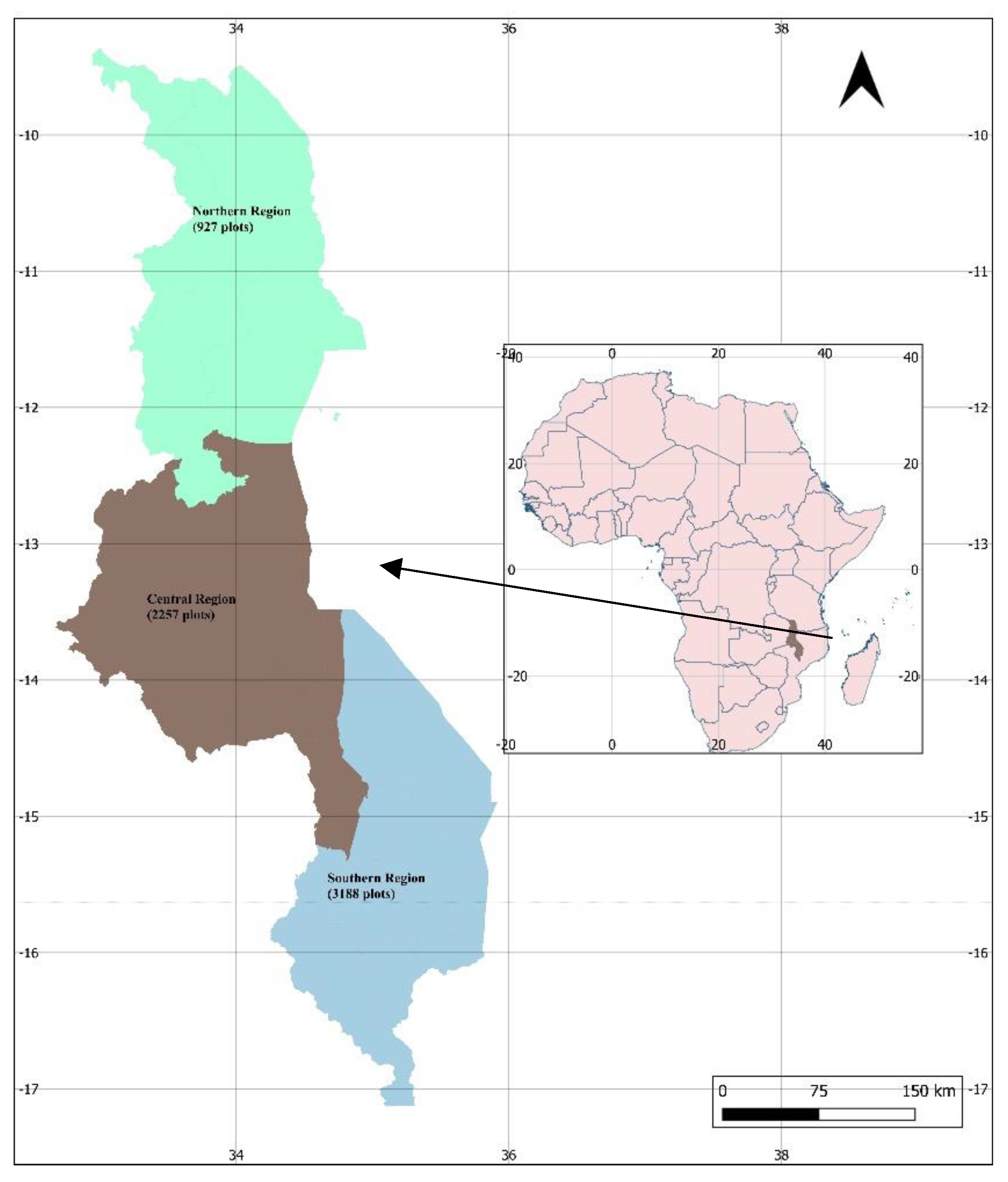
Figure 2.
Technical Efficiency by Soil Quality and Erosion Rate.
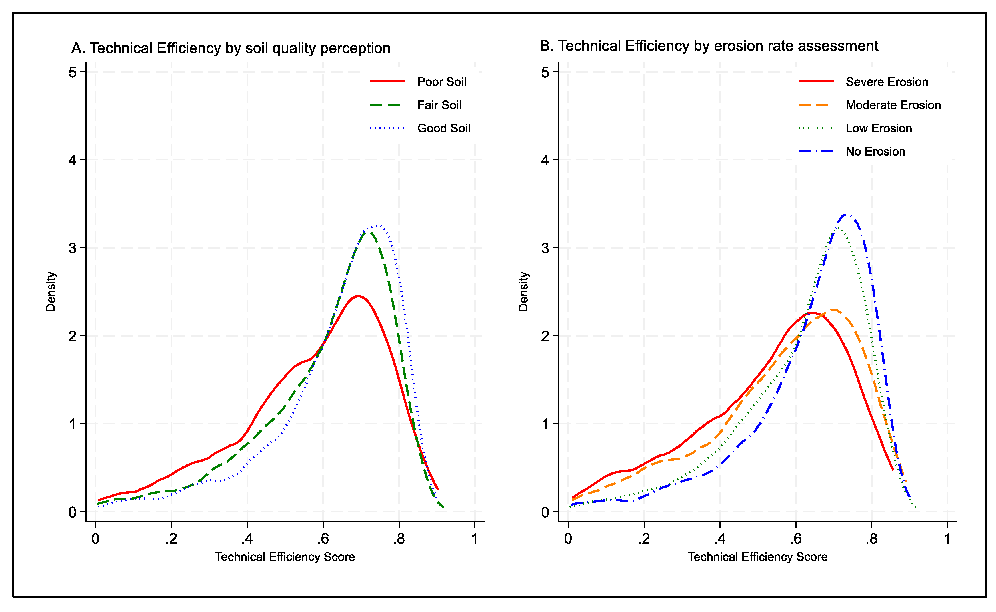

Table 1.
Variable Definition, Description and Measurement Units.
| Variable | Description | Measurement unit |
|---|---|---|
| Crop productivity | Total maize output obtained from the plot | Kg |
| Plot area | Total area of the cultivated plot | Acres |
| Organic fertilizer | Quantity of organic manure or compost applied to the plot. | Kg |
| Inorganic fertilizer | Quantity of chemical fertilizer applied to the plot. | Kg |
| Labour | Total household and hired labour used on the plot. | Man-hours |
| Seed quantity | Total seed used for planting the plot. | Kg |
| Pesticides/herbicides use | Indicates whether a farmer applied pesticide or herbicide during the production season. | 1=Yes; 0=No |
| Improved variety | Indicates whether an improved maize seed variety was planted. | 1 = Improved variety; 0 = Local |
| Soil quality | Farmer’s subjective assessment of soil fertility condition. | 1 = Poor; 2 = Fair; 3 = Good |
| Soil erosion rate | Self-reported rate of soil erosion observed on the plot. | 1 = Severe ; 2 = Moderate; 3 = Low; 4 = No erosion |
| Agro-ecological zone | Climatic zone determined by temperature and rainfall regime. | 1 = Tropic-warm/semi-arid; 2 = Tropic-warm/sub-humid; 3 = Tropic-cool/semi-arid; 4 = Tropic-cool/sub-humid |
| Region | Administrative region where the plot is located. | 1 = Northern; 2 = Central; 3 = Southern |
| Extension contact on inorganic fertilizer | Household received extension advice on inorganic fertilizer use. | 1 = Yes; 0 = No |
| Extension contact on organic fertilizer | Household received extension advice on organic fertilizer. | 1 = Yes; 0 = No |
| Extension contact on seed variety | Household received extension advice on improved seeds. | 1 = Yes; 0 = No |
| Fertilizer coupon | Household accessed government fertilizer subsidy. | 1 = Yes; 0 = No |
| Livestock ownership | Household owns livestock. | 1 = Yes; 0 = No |
| Household size | Number of household members residing in the household. | Number of persons |
Table 2.
Mean input allocation and maize output per plot (n=6,370).
| Variable | Mean | Linearised Standard Error |
|---|---|---|
| Plot area (acres) | 0.88 | 0.01 |
| Seeds (kg) | 7.70 | 0.08 |
| Organic fertilizer (kg) | 208.02 | 48.17 |
| Fertilizer total | 56.02 | 0.77 |
| Labour man-hours | 31.26 | 0.28 |
| Pesticides | 0.04 | 0.003 |
| Variety | 0.48 | 0.01 |
| Maize output (kg) | 442.20 | 8.85 |
Note: Plot-level means estimated using survey weights (svy).
Table 3.
Estimated effects from CMP regression models (probit, censored Tobit and Linear) for input decisions among maize farmers.
Table 3.
Estimated effects from CMP regression models (probit, censored Tobit and Linear) for input decisions among maize farmers.
| Variable | Pesticide use | Improved variety | Organic Fertiliser (ln) | Inorganic Fertiliser (ln) | Labour hours (ln) |
|---|---|---|---|---|---|
| Soil quality | Probit (dy/dx) | Probit (dy/dx) |
Censored Tobit (Coefficient) | Linear (Coefficient) | Linear (Coefficient) |
| Fair | 0.05 (0.06) |
-0.04 (0.04) | 0.24 (0.22) |
-0.11*** (0.03) |
-0.07 (0.02) |
| Poor | 0.01 (0.09) |
-0.03 (0.05) | 0.57* (0.31) |
-0.22*** (0.04) |
-0.14** (0.01) |
| Soil erosion | |||||
| Low | 0.09 (0.06) |
-0.01 (0.04) | 0.56** (0.23) |
0.02 (0.52) |
0.09 (0.03) |
| Moderate | -0.02 (0.10) | -0.12** (0.06) | 0.57 (0.35) |
0.03 (0.04) |
0.11 (0.02) |
| High | 0.14 (0.11) |
-0.11 (0.07) |
-0. 16 (0.45) |
0.09 (0.27) |
0.09 (0.02) |
| Region | |||||
| Central | -0.02 (0.12) | -0.13** (0.08) | |||
| Southern | -0.07 (0.11) | -0.51*** (0.07) | |||
| Extension on pest control | 0.31*** (0.06) | ||||
| Agro-ecological zone | |||||
| Tropic-warm/subhumid | 0.22*** (0.07) | -0.11*** (0.04) | -0.787*** (0.22) |
-0.23*** (0.04) |
0.13*** (0.02) |
| Tropic-cool/semi arid | -0.01 (0.01) | -0.26*** (0.05) | -1.63*** (0.33) |
0.24*** (0.03) |
0.09** (0.02) |
| Tropic-cool/subhumid | 0.19 (0.14) |
-0.12 (0.08) | -3.50*** (0.42) |
0.67*** (0.04) |
0.04 (0.02) |
| Extension on new seed varieties | 0.27*** (0.04) | ||||
| Livestock ownership | 0.04 (0.22) |
||||
| Extension on organic fertilizer | 1.66*** (0.21) |
||||
| Extension on inorganic fertilizer use | 0.10*** (0.03) |
||||
| Inorganic fertilizer coupon | 0.10*** (0.03) |
||||
| Household size | 0.11*** (0.01) |
||||
| Observations | 6370 | 6370 | 6370 | 6370 | 6370 |
Notes: Estimates are from the CMP model. Standard errors are in parentheses. *, ** and *** denote significance at 10%, 5% and 1% levels, respectively. Reference groups: soil quality = Good; erosion = No erosion; region = Northern; agro-ecological zone = Tropic-warm/semiarid.
Table 4.
The stochastic production frontier and inefficiency model for maize output.
| Crop productivity | Production function | Inefficiency model |
|---|---|---|
| Acreage (ln) | 0.24 (0.02) |
|
| Pesticides | 0.14** (0.04) |
|
| Improved variety | 0.22*** (0.02) |
|
| Seed(ln) | 0.33*** (0.02) |
|
| Inorganic fertiliser (ln) | 0.47*** (0.01) |
|
| Organic fertilizer (ln) | 0.01*** (0.003) |
|
| Labour (ln) | 0.08 (0.02) |
|
| Soil quality: | ||
| Fair | 0.19*** (0.0.07) |
|
| Poor | 0.42*** (0.10) |
|
| Soil erosion: | ||
| Low | 0.11 (0.08) |
|
| Moderate | 0.49*** (0.11) |
|
| High | 0.68*** (0.13) |
|
| Constant (ln σ²ᵤ) | 5.222** (1.529) |
|
| Constant (ln σ²ᵥ) | 11.932*** (0.018) |
Notes: Standard errors are in parentheses. Reference groups: soil quality = Good; erosion = No erosion. *, ** and *** denote significance at 10%, 5%, and 1% levels, respectively.
Table 5.
ANOVA results of Technical Efficiency by soil quality and erosion rate.
| Soil assessment | Technical Efficiency | ANOVA p-value | ||||
|---|---|---|---|---|---|---|
| N | Mean | p25 | p50 | p75 | ||
| A. Soil quality | ||||||
| Poor | 836 | 0.57 | 0.47 | 0.62 | 0.72 | 0.000 |
| Fair | 2,041 | 0.61 | 0.52 | 0.66 | 0.74 | |
| Good | 3,493 | 0.64 | 0.66 | 0.68 | 0.76 | |
| B. Erosion rate | ||||||
| Severe | 366 | 0.54 | 0.41 | 0.58 | 0.68 | 0.000 |
| Moderate | 579 | 0.57 | 0.46 | 0.61 | 0.72 | |
| Low | 1,750 | 0.62 | 0.53 | 0.66 | 0.74 | |
| No erosion | 3,675 | 0.64 | 0.57 | 0.68 | 0.76 | |
| Total | 6,370 | 0.62 | ||||
Disclaimer/Publisher’s Note: The statements, opinions and data contained in all publications are solely those of the individual author(s) and contributor(s) and not of MDPI and/or the editor(s). MDPI and/or the editor(s) disclaim responsibility for any injury to people or property resulting from any ideas, methods, instructions or products referred to in the content. |
| 1 | The model was estimated using sfcross Stata command (Belotti et al., 2013)(Belotti et al., 2013) |
© 2026 by the authors. Licensee MDPI, Basel, Switzerland. This article is an open access article distributed under the terms and conditions of the Creative Commons Attribution (CC BY) license (http://creativecommons.org/licenses/by/4.0/).
Copyright: This open access article is published under a Creative Commons CC BY 4.0 license, which permit the free download, distribution, and reuse, provided that the author and preprint are cited in any reuse.


