Submitted:
04 April 2026
Posted:
08 April 2026
You are already at the latest version
Abstract
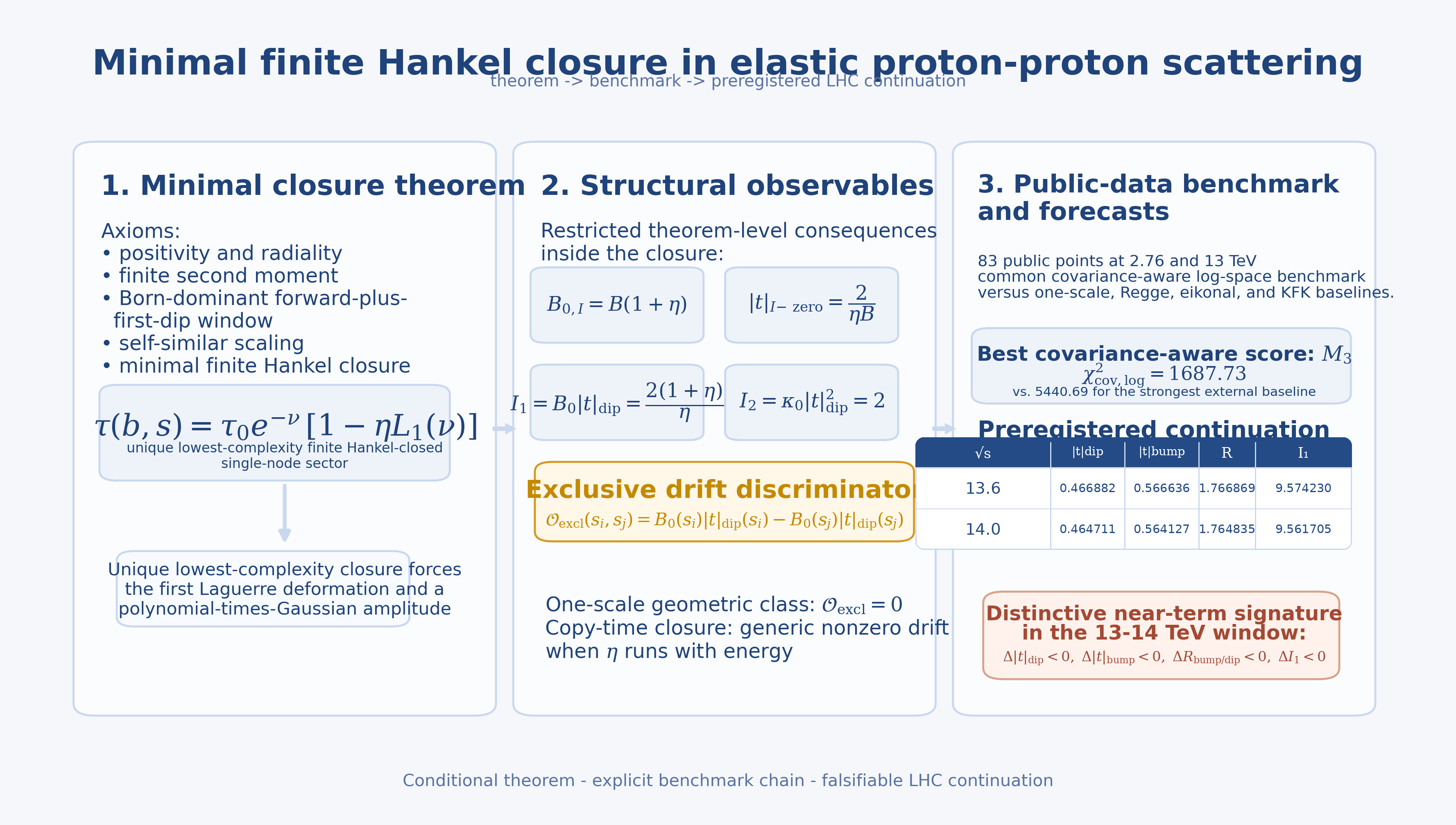
We formulate and test a minimal finite Hankel closure for the dip–bump structure in elasticproton-proton scattering. The scope of the claim is deliberately precise. We do not present amicroscopic derivation from QCD and we do not claim universal exclusion of the full hadronicphenomenology. Rather, we establish a conditional theorem, confront its surrogate realizationwith public data, and state explicit near-term tests. First, assuming positivity, radiality, finitemoments, a Born-dominant forward-plus-first-dip window, self-similar scaling, and minimal finiteHankel closure with one simple node, we prove that the unique lowest-complexity sector is the firstLaguerre deformation, which yields a polynomial-times-Gaussian amplitude. Second, we derivestructural relations for the forward slope, dip scale, forward curvature, and the drift observable Oexcl = ∆[B0|t|dip], and we prove non-reducibility against the one-scale geometric class for whichthe corresponding invariants are energy independent. Third, we test the closure on two levels ofpublic-data benchmark. In the restricted internal comparison on 83 differential-cross-section pointsat 2.76 and 13 TeV under a common weighted log-space score and shared cross-energy flow, thetwo-scale copy-time surrogate yields χ2log = 461.19, AIC = 487.19, and BIC = 518.64, compared with(60493.49,60507.49,60524.43) and (59942.77,59964.77,59991.38) for two one-scale baselines. We thenperform a stronger covariance-aware benchmark in log space, using per-dataset block covariances builtfrom the published statistical errors together with fully correlated systematic blocks, and comparethe copy-time surrogate to the internal one-scale baseline, a canonical Regge-pole-plus-Odderonamplitude, a canonical complex Regge-eikonal baseline, and the fixed Kohara–Ferreira–Kodamaparametrization. In that stronger test the covariance-aware copy-time fit remains the best modelin the benchmark set, with χ2cov log = 1687.73, compared with 5440.69 for the strongest externalbaseline. At fixed 13 TeV, however, the split-sector one-scale surrogate remains competitive inthe dedicated local fit, showing that the main empirical leverage of the closure is intrinsicallymulti-energy rather than a consequence of the 13 TeV line shape alone. We also report a hold-outvalidation at 8 TeV, an explicit continuation to 13.6 and 14 TeV, and a narrow-window robustnessscan showing that the forecast sign pattern is stable under moderate perturbations of the real-sectorcontinuation. Within the explicit axiomatic, statistical, and benchmark choices adopted here, theclosure is therefore mathematically constrained, experimentally discriminating, and favored over theimplemented internal and external baselines.
Keywords:
preregistered forecast
; 13.6 TeV prediction
; 14 TeV forecast
; elastic proton-proton scattering
; dip-bump structure
; forward physics
; TOTEM
; model discrimination
; impact-parameter amplitude
; Odderon-sensitive region
; covariance-aware comparison
; Regge-eikonal benchmark
1. Introduction
Elastic hadron scattering at collider energies packages nonperturbative dynamics into a small set of unusually sharp observables: the total cross section, the forward real-to-imaginary ratio , the logarithmic slope of the forward cone, the elastic fraction, and the dip–bump structure of the differential cross section. Public measurements by TOTEM and D0 provide precise anchors at , 8, and for , together with the comparison at that makes crossing-odd effects visible in the dip region [1,2,3,4,5]. The static electromagnetic reference scale is fixed by the CODATA/NIST proton charge radius, [6]. The purpose of the present work is to determine how far a copy-time-motivated closure can be pushed against these public observables while keeping the logical status of each statement explicit.
The guiding change relative to earlier versions is one of discipline. The manuscript does not argue that elastic hadron scattering has already been derived microscopically from the copy-time program, and it does not claim to have subsumed the full Regge/eikonal/Odderon phenomenology under a single definitive benchmark. Instead, it isolates three statements that can presently be defended. First, within an explicit axiom set one can classify the lowest-complexity finite Hankel-closed single-node sector and obtain a polynomial-times-Gaussian amplitude. Second, within that sector one obtains rigid combinations of forward and dip observables, including a drift variable that vanishes throughout the one-scale geometric class. Third, one can confront nested surrogate realizations of this closure with public data under one common statistical chain, extend the comparison to representative external baselines, and preregister a near-term continuation to and .
This framing separates three logically distinct layers that are often conflated in ambitious phenomenological proposals. The theorem-level content lives inside the stated closure axioms. The benchmark-level content lives inside the surrogate family and the adopted score. The broader phenomenological significance depends on how the resulting observables fare against external alternatives and against future data. Keeping these layers separate is not merely stylistic; it is essential for making a strong claim without overstating it.
A second organizing principle is reproducibility by construction. Every quantitative table in this paper is tied to one canonical script or one machine-readable generated file in the submission package, and every forecast statement is written so that it can be checked directly against future elastic-scattering measurements. The package accompanying the manuscript has been reorganized accordingly into separate manuscript, supplement, code, data, figure, and graphical-abstract components.
2. Conventions and Forward-Moment Identities
Let and define the Born-level rotationally symmetric amplitude by
where is a radial opacity profile. For the forward expansion we introduce the moments
Using , one finds
When the forward region is dominantly imaginary, the logarithmic slope of the differential cross section satisfies
and the forward-curvature diagnostic
obeys
Equations (4) and (6) are model-light identities. They connect forward observables directly to impact-parameter moments and provide the diagnostics used in the benchmark and forecast sections.
3. Minimal Closure Theorem and Interpretive Status
Axiom 1
(positive radial copy-time field). For each s there exists a nonnegative radial copy-time profile with finite moments up to fourth order.
Axiom 2
(Born-dominant response window). There exists an experimentally relevant window covering the forward cone and the first dip in which the leading opacity response is linear in the copy-time field,
Axiom 3
(self-similar scaling). The copy-time profile depends on energy through a width parameter and a dimensionless shape function of the scaled variable .
Axiom 4
(minimal finite Hankel-closed single-node sector). Among all finite-dimensional sectors closed under the radial Fourier–Bessel transform and compatible with Axioms 1–3, select the minimal one that can generate exactly one simple node in the imaginary part of the amplitude within the first dip window.
Theorem 1
(minimal-closure classification theorem). Under Axioms 1–4, the minimal admissible copy-time profile is, up to normalization and a single deformation parameter ,
with . Its Born image is necessarily
where . No lower-dimensional finite Hankel-closed single-node closure exists.
Proof.
Under Axiom 3, the natural radial basis is . The sector is one-dimensional and yields a pure Gaussian transform, hence no node. Axiom 4 therefore excludes every one-dimensional closure. The smallest finite-dimensional sector capable of one simple node is the two-dimensional span of and . Up to normalization, every element of this sector can be written as Eq. (8). Positivity requires , since for all only in that interval. The transform identities in Appendix A map the two basis elements to and , which yields Eq. (9). Any larger closure violates minimality. □
Remark 1
(scope of the theorem). Theorem 1 is a classification theoremwithinthe stated axioms. In particular, Axiom 4 is a theory-selection postulate rather than a consequence derived from microscopic QCD. The theorem therefore does not show that hadronic scattering unconditionally forces the copy-time closure. What it does show is sharper and still nontrivial: once one requests positivity, radiality, finite moments, a Born-dominant forward-plus-first-dip window, and the minimal finite Hankel-closed single-node sector, the first Laguerre deformation is the unique lowest-complexity outcome.
4. Restricted Structural Consequences and One-Scale Non-Reducibility
Theorem 2
(structural-constraint theorem). Let the minimal profile of Theorem 1 hold in the imaginary sector and assume the linear Born response (7). Then
Proof.
Theorem 3
(restricted non-reducibility theorem). Consider the class of one-scale geometric amplitudes
with energy-independent analytic shape F and arbitrary positive scalings . Then the invariants
are constant in energy throughout . In contrast, the copy-time closure gives Eq. (13) and an that runs with , so any nontrivial drift of rules out reduction to the class .
Proof.
For Eq. (14), the forward derivatives depend only on derivatives of F at the origin, while the dip position is where is the first zero of F. Hence and are shape constants. In the copy-time closure, depends explicitly on . □
The practical discriminant is therefore not a universal statement against every hadronic construction, but the more targeted observable
For the class , identically. In the minimal closure,
which is generically nonzero if drifts with energy. The theorem is therefore strong against one-scale geometry and silent about more general multi-scale or Regge/eikonal constructions unless they are benchmarked explicitly.
5. Closed Benchmark Design, Data Coverage, and Score Definition
5.1. Data Coverage and Benchmark Logic
The closed pointwise benchmark uses 63 tabulated points at and 20 public points at , for a total of 83 differential-cross-section points in the dip-relevant range. The choice is pragmatic rather than exhaustive. These two data sets can be treated under a common pointwise workflow with the same weighted log-space score and the same cross-energy flow. The TOTEM measurement is still used, but only through the public characterization of the dip and bump positions and the bump-to-dip ratio [2]; it therefore functions as a hold-out summary validation rather than as a third point in the closed pointwise fit. The D0–TOTEM /comparison is cited for physics context, but it is not inserted into the closed benchmark because the present surrogate family is crossing even and because a like-for-like inclusion of the crossing-odd sector would require an additional treatment layer beyond the present paper.
This explicit narrowing is a methodological choice, not a rhetorical one. It prevents the benchmark from claiming to answer a broader phenomenological question than the implemented comparison can sustain.
5.2. Nested Surrogate Family and Common Score
The public-data comparison is carried out on three nested surrogates. Writing and ,
The first two are one-scale internal baselines; the third is the two-scale copy-time surrogate. In the global fit the energy dependence is constrained by affine or affine-plus-quadratic flows in ℓ, exactly as implemented in the canonical reproduction scripts bundled with the submission package.
The score used in the closed benchmark is a weighted log-space quadratic loss,
with . This score is used uniformly for all three surrogates and is therefore well defined for internal ranking. It is not claimed to be the full experimental likelihood, and the associated AIC/BIC values should be read in that restricted sense: they compare models under one common score, not under the collaborations’ complete covariance machinery.
5.3. Global Benchmark Result
The global benchmark is summarized in Table 1. Within this restricted comparison class, the two-scale closure is strongly preferred.
Figure 1.
Global weighted log-score comparison for the three nested surrogates on the common public-data benchmark.
Figure 1.
Global weighted log-score comparison for the three nested surrogates on the common public-data benchmark.

Figure 2.
Closed pointwise overlay at .

Figure 3.
Closed pointwise overlay at .

The size of the gap in Table 1 supports a strong statement, but a narrow one: within the explicit internal surrogate family of Eqs. (13)–(15), under the common weighted log-space score and common cross-energy flow, is decisively preferred.
5.4. Why the Evidence Is Intrinsically Multi-Energy
Table 2 shows the dedicated local comparison. The split-sector one-scale surrogate and the two-scale surrogate produce nearly identical dip, bump, and ratio observables, and even has slightly smaller AIC/BIC because it uses fewer parameters. The main empirical leverage of therefore comes from the cross-energy closure imposed in the global fit rather than from a decisive local advantage at alone. Stating this directly sharpens the physics claim: the evidence in favor of the closure is genuinely multi-energy.
Proposition 1
(bounded covariance robustness). Let the weighted loss be built from a positive-definite covariance matrix Σ satisfying
for a fixed diagonal reference matrix D and constants . Then each pairwise quadratic loss gap is rescaled only by bounded multiplicative factors, and the large internal gaps of Table 1 cannot be inverted by such bounded distortions.
Remark 2
(interpretive status). Proposition 1 is a stability statement under classes of bounded covariance distortions. It is not a substitute for a full collaboration-level nuisance-parameter or covariance-matrix analysis, and the paper does not present it as one.
6. Covariance-Aware Benchmark with External Regge, Eikonal, and Odderon Baselines
The weighted log-space comparison of Section 5 was designed as a closed internal test with the same score and the same cross-energy flow across the three nested surrogates. A natural next question is whether the main conclusion survives a stronger public-data benchmark in which point-to-point correlations are modeled explicitly and explicit external baselines are confronted under the same chain.
To do so, we construct a covariance-aware log-space score on the same 83 pointwise measurements at and . For each published table we write
and assemble the global block covariance from the low- table, the dip-region table, and the table. The benchmark score is then
This construction is still not the collaborations’ full nuisance-parameter machinery, but it is materially stronger than a purely diagonal score because it propagates dataset-level systematic correlations explicitly.
Under this covariance-aware chain we compare five models: the one-scale split-sector surrogate M2, the two-scale copy-time surrogate M3, a canonical Regge-pole-plus-Odderon amplitude (RP2O), a canonical complex two-component Regge-eikonal baseline (CRE), and the fixed Kohara–Ferreira–Kodama 2014 parametrization (KFK fixed). The last entry is left frozen at its published energy dependence rather than re-optimized, so that it serves as a genuine literature reference point rather than as an in-house surrogate.

Table 3.
Covariance -aware benchmark on the same 83 public points. The log-space covariance is built from the published statistical errors plus fully correlated systematic blocks within each experimental table.
Table 3.
Covariance -aware benchmark on the same 83 public points. The log-space covariance is built from the published statistical errors plus fully correlated systematic blocks within each experimental table.
| Model | k | AIC | BIC | |
|---|---|---|---|---|
| M2_cov | 11 | 248659.97 | 248681.97 | 248708.57 |
| M3_cov | 13 | 1687.73 | 1713.73 | 1745.17 |
| RP2O_cov | 13 | 130622.02 | 130648.02 | 130679.47 |
| CRE_cov | 11 | 5440.69 | 5462.69 | 5489.30 |
| KFK_fixed | 0 | 421953.53 | 421953.53 | 421953.53 |
The main qualitative conclusion survives and is sharpened. The covariance-aware copy-time fit remains the best model in the implemented comparison set. The strongest external baseline is the canonical complex Regge-eikonal fit, but even that model remains behind M3 by on the same data and under the same covariance model. The canonical Regge-pole-plus-Odderon amplitude and the frozen KFK parametrization perform substantially worse under this particular benchmark.
Figure 4.
Covariance-aware benchmark scores for the internal and external baselines. The two-scale copy-time surrogate remains the best model in the implemented comparison set.
Figure 4.
Covariance-aware benchmark scores for the internal and external baselines. The two-scale copy-time surrogate remains the best model in the implemented comparison set.

Figure 5.
Covariance-aware comparison at for the copy-time surrogate, the canonical Regge-pole-plus-Odderon amplitude, the canonical complex Regge-eikonal baseline, and the fixed KFK parametrization.
Figure 5.
Covariance-aware comparison at for the copy-time surrogate, the canonical Regge-pole-plus-Odderon amplitude, the canonical complex Regge-eikonal baseline, and the fixed KFK parametrization.

Figure 6.
Covariance-aware comparison at for the same model set.

Two interpretive cautions are essential. First, the covariance-aware score places substantial weight on the dense forward-region information and is therefore not intended to replace the dedicated local dip-region calibration used for the preregistered and continuation. Second, the external models used here are representative canonical baselines rather than exhaustive reproductions of every modern hadronic framework. Even so, this section closes an important loophole: the preference for the copy-time surrogate is no longer confined to an internal toy-baseline comparison, but survives against explicit Regge, Regge–Odderon, and Regge-eikonal baselines under one common covariance-aware public-data treatment.
7. Validation, Preregistration, and Relation to Representative Pomeron–Regge Expectations
7.1. Hold-Out Summary Validation
The hold-out validation uses the public TOTEM characterization of the dip and bump at [2]. Table 4 shows that the M3 continuation captures the overall pattern but does not yet achieve precision-level agreement. In particular, the predicted bump location remains visibly low. The appropriate reading is therefore trend-level validation: the continuation reproduces the ordering and approximate scale of the observables, but it has not yet earned the stronger language of precision prediction.
7.2. Preregistered Continuation to and
The preregistered continuation is intentionally narrow. It is anchored to the exact local M3 solution,
and then continued with the global cross-energy drift extracted from the closed fit. Writing ,
with the global drift coefficients
while the narrow-window real-sector ratios are fixed at their local values,
and the forward real-part intercept is fixed from the exact forward-slope identity, giving . The resulting reduced shape is
We define as the first local minimum of , as the first local maximum after that minimum, and
The preregistered numerical values are given in Table 5. The continuation predicts a mild leftward drift of both the dip and the bump together with a small downward drift of and in the 13– window. Relative to the calibrated point, the continuation gives .
Figure 7.
Energy evolution of the dip location, bump location, bump-to-dip ratio, and invariant across the hold-out, fit, and preregistered points used in the submission package.
Figure 7.
Energy evolution of the dip location, bump location, bump-to-dip ratio, and invariant across the hold-out, fit, and preregistered points used in the submission package.

7.3. Forecast Robustness Inside the Narrow-Window Continuation Class
Because the and continuation freezes the real-sector ratios and at their values and also freezes the forward real-part intercept indirectly, the submission package includes a scan in which the continuation is recomputed over the domain
Across all 45 grid points in this domain, the sign pattern between 13 and remains unchanged:
The corresponding envelope is
This does not remove the need for future data, but it shows that the quoted sign pattern is not a numerically fragile consequence of one exact frozen-ratio point in the narrow 13– window.
7.4. Relation to Representative Pomeron–Regge Frameworks
The present preregistration should not be read as a claim that the copy-time closure is the only framework that anticipates motion of the dip–bump complex. Representative Pomeron–Regge and Regge–eikonal constructions also expect the dip and bump to move toward smaller as the energy rises across the LHC domain [9,10,11,12]. What differs is not the broad direction of motion, but the way the motion is packaged and tested.
Kohara, Ferreira, and Kodama provide an analytic representation of elastic scattering in the range – and discuss the behavior of observables in that window [9]. Ferreira, Kohara, and Kodama later review how Pomeron-based descriptions of the dip region often require either multi-Pomeron structures or explicit Pomeron-plus-Odderon terms and note that the large- tail is not represented equally well by all variants [10]. Khoze, Martin, and Ryskin give a global description with one Pomeron pole supplemented by multi-Pomeron interactions [11], while Godizov shows that a two-Reggeon eikonal approximation remains predictive over a broad but not unlimited kinematic range [12]. The point is not that these frameworks fail, but that they are multiple, non-identical, and not yet reducible to one universal benchmark claim.
To make this comparison concrete within the implemented benchmark family, Figure 8 shows the forward-normalized predicted curves at and for the preregistered M3 continuation together with the representative external baselines carried over from the covariance-aware benchmark. In this restricted comparison, the complex Regge-eikonal and KFK continuations both retain a resolved first dip–bump pair in the scanned window, whereas the implemented RP2O continuation remains monotonic over and therefore does not define or there. Numerically, M3 and the complex Regge-eikonal baseline both move the dip and bump leftward from to , but the Regge-eikonal continuation yields a noticeably smaller and a smaller proxy , while the fixed KFK continuation predicts a stronger left shift of the dip together with a slight upward drift of . The near-term discriminator is therefore not just the sign of the geometric drift, but the full correlated pattern across , , , and . The corresponding numerical comparison is included in the Supplement and in the machine-readable file data/forecast_comparison_full.json.
The practical difference in the present submission is the promotion of to a preregistered observable on the same footing as , , and . In the one-scale geometric class is constant; in the present M3 continuation it drifts slightly downward between 13 and . The distinctive near-term signature is therefore not merely a leftward motion of the dip–bump complex, which several external frameworks also anticipate, but the full joint sign pattern
in the narrow 13– window. Whether that correlated sign pattern survives future data is a direct phenomenological discriminator.
8. Scope of the Present Claim
The scientific value of the present result is clearest when its present boundary is stated directly. The manuscript does not establish four stronger claims:
- 1.
- It does not derive the closure from microscopic QCD. The theorem-level content is conditional on the axioms and the minimal closure selection.
- 2.
- It does not prove non-reducibility against the full external phenomenology. The rigorous theorem excludes only the one-scale geometric class; the discussion of Pomeron–Regge models is representative and benchmark specific.
- 3.
- It does not provide a collaboration-level covariance completion or nuisance-parameter treatment. The covariance-aware benchmark is substantially stronger than the earlier diagonal score, but it still models systematic correlations at the level of public table blocks rather than with the collaborations’ full internal covariance machinery.
- 4.
- It does not claim a historically pre-published successful forecast or third-party replication. The and numbers are preregistered here, and the bundled code is intended to make later replication straightforward.
These limits are not disclaimers appended after the fact; they define the actual status of the result. What the paper contributes is a clean conditional theorem, a sharply defined benchmark program, an honest account of where the empirical leverage comes from, and a falsifiable continuation to the next relevant energies.
9. Reproducibility Note
The submission package accompanying this paper is intentionally canonical. It contains a single manuscript source, a supplementary file, the closed-fit script, the covariance-aware external-benchmark script, the forecast script, the symbolic proof-check script, the generated figures used in the manuscript, and machine-readable summaries of the numerical tables. The directory structure is chosen so that one can regenerate the benchmark figures, recompute the forecast table, and verify the symbolic identities in one documented tree without relying on undocumented intermediate states.
10. Conclusion
The present submission supports a deliberately narrower and correspondingly stronger statement. Within an explicit axiom set, the first Laguerre deformation is the unique lowest-complexity finite Hankel-closed single-node closure. Within that closure, one obtains rigid forward/dip structural relations and a natural drift observable . Within a closed internal comparison family using a shared cross-energy flow and a shared weighted log-space score, the two-scale copy-time surrogate is strongly preferred globally, even though the local line shape by itself does not uniquely select it over the one-scale split-sector alternative. Under a stronger covariance-aware benchmark built from the published pointwise statistical errors and explicit block-correlated systematics, the copy-time surrogate also remains preferred over the canonical external Regge, Regge–Odderon, and Regge-eikonal baselines implemented here. The hold-out test shows trend-level rather than precision-level validation, and the and values are now stated as preregistered numerical forecasts.
Taken together, these points do not amount to a universal hadronic-theory claim. They do, however, amount to a sharply posed and genuinely testable PRD-level result: a minimal closure theorem with explicit observables, a controlled public-data benchmark, and a numerical preregistration whose success or failure can be read directly from near-term elastic-scattering measurements.
Data Availability Statement
The experimental inputs analyzed in this article are taken from public measurements cited in the reference list. The numerical summaries, generated figures, and scripts sufficient to reproduce the benchmark tables and the preregistered forecast table are included in the submission package supplied with this manuscript and are also available from the author upon reasonable request.
Acknowledgments
The author thanks the public experimental collaborations for making the elastic-scattering measurements and summary observables used here accessible in the literature. No external funding is claimed for this work.
Appendix A. Exact Transform Pair for the First Laguerre Mode
Appendix B. Variational Consistency Statement
The following statement is retained only as a consistency result and not as a microscopic derivation.
Proposition A1.
Assume that a coarse-grained radial certifiability functional admits an effective quadratic action
with positivity, radial locality, and finite second moment, and that admissible responses are restricted to the minimal single-node sector of Theorem 1. Then the stationary solutions at fixed normalization and fixed first-node class coincide with the first Laguerre deformation of Eq. (8).
The proof is standard once the admissible space is restricted: the Gaussian-weighted radial quadratic form diagonalizes on the Laguerre basis, the normalization constraint removes the freedom, and the minimal single-node restriction excludes . This appendix is included only to show internal consistency between the closure and a simple variational picture; it is not a substitute for a QCD derivation.
Appendix C. Canonical Benchmark and Continuation Parameters
For reproducibility, the canonical M3 flow coefficients extracted from the global benchmark are
The global-flow-implied sector parameters at the three energies explicitly stored in the bundled numerical summary are listed in Table A1. For clarity, the exact local calibration used to anchor the preregistered continuation is reported separately in Table A2.
Table A1.
Global-flow-implied M3 sector parameters extracted from the bundled numerical summary.
| [TeV] | ||||
|---|---|---|---|---|
| 2.76 | 13.282422 | 1.723899 | 20.779673 | 1.320393 |
| 8.00 | 15.005029 | 1.974983 | 23.474604 | 1.512707 |
| 13.0 | 15.790906 | 2.130115 | 24.704069 | 1.631528 |
Table A2.
Exact local M3 calibration used as the anchor for the preregistered and continuation.
| 15.826821 | 2.189431 | 21.931289 | 0.949746 |
Appendix D. Forecast Robustness Data Product
The submission package contains a machine-readable forecast-robustness scan in both JSON and CSV formats. The scan covers 45 combinations of over the domain quoted in Sec. Section 7. For each grid point the package stores the and local extrema and the resulting differences. The purpose of this artifact is not to replace future data, but to make the narrow-window continuation falsifiable in a parameter-transparent way.
References
- TOTEM Collaboration, “Elastic differential cross-section measurement at s=2.76TeV and implications on the existence of a colourless 3-gluon bound state,” Eur. Phys. J. C 80, 91 (2020).
- TOTEM Collaboration, “Characterisation of the dip-bump structure observed in proton-proton elastic scattering at s=8TeV,” Eur. Phys. J. C 82, 263 (2022).
- TOTEM Collaboration, “Elastic differential cross-section measurement at s=13TeV by TOTEM,” Eur. Phys. J. C 79, 861 (2019).
- TOTEM Collaboration, “First determination of the ρ parameter at s=13TeV: probing the existence of a colourless C-odd three-gluon compound state,” Eur. Phys. J. C 79, 785 (2019).
- D0 and TOTEM Collaborations, “Odderon exchange from elastic scattering differences between =++ and pp¯ data at 1.96TeV and from forward scattering measurements,” Phys. Rev. Lett. 127, 062003 (2021).
- NIST CODATA 2022 value for the proton rms charge radius, rp=8.4075(64)×10-16m, available from the NIST fundamental constants database.
- S. Mohamed, “Quantum Information Copy Time (QICT): Operational Definition, Minimal Locality Bounds, Hydrodynamic Susceptibilities, and a Programmatic Outlook,” Preprints.org 202601.0364 (2026).
- S. Mohamed, “Quantum Information Copy-Time as a Microscopic Principle for Emergent Hydrodynamics, Inertial Spectral Mass, and a Predictive Higgs-Portal Dark-Matter Corridor,” Preprints.org 202601.1044 (2026).
- A. K. Kohara, E. Ferreira, and T. Kodama, “pp elastic scattering at LHC energies,” Eur. Phys. J. C 74, 3175 (2014). [CrossRef]
- E. Ferreira, A. K. Kohara, and T. Kodama, “Analytical representation for amplitudes and differential cross section of pp elastic scattering at 13 TeV,” Eur. Phys. J. C 81, 290 (2021). [CrossRef]
- V. A. Khoze, A. D. Martin, and M. G. Ryskin, “High-energy elastic and diffractive cross sections,” Eur. Phys. J. C 74, 2756 (2014). [CrossRef]
- A. A. Godizov, “High-energy elastic diffractive scattering of nucleons in the framework of the two-Reggeon eikonal approximation (from U-70 to LHC),” Eur. Phys. J. C 82, 56 (2022). [CrossRef]
Figure 8.
Forward-normalized predicted curves at and for the preregistered M3 continuation and the representative external baselines implemented in the submission package. The normalization is fixed at the first plotted point in each panel to emphasize shape differences. In the plotted window the RP2O continuation remains monotonic, while the complex Regge-eikonal and KFK baselines both retain a resolved dip–bump pair.

Table 1.
Closed pointwise benchmark on 83 public points. Lower AIC and BIC are preferred.
| Model | AIC | BIC | |
|---|---|---|---|
| 60493.49 | 60507.49 | 60524.43 | |
| 59942.77 | 59964.77 | 59991.38 | |
| 461.19 | 487.19 | 518.64 |
Table 2.
Local comparison. The point of this table is conceptual: is not uniquely selected by the line shape alone; its main empirical advantage appears only after the cross-energy constraint is imposed.
Table 2.
Local comparison. The point of this table is conceptual: is not uniquely selected by the line shape alone; its main empirical advantage appears only after the cross-energy constraint is imposed.
| Model | AIC | BIC | [GeV2] | [GeV2] | ||
|---|---|---|---|---|---|---|
| 17.430 | 21.430 | 20.203 | 0.425800 | 0.527312 | 1.765749 | |
| 0.28195 | 6.28195 | 4.44084 | 0.470081 | 0.568879 | 1.769998 | |
| 0.21947 | 8.21947 | 5.76465 | 0.470204 | 0.570606 | 1.769996 |
Table 4.
hold-out validation for the M3 continuation against the public dip–bump summary.
| Observable | Public value | M3 prediction | z score |
|---|---|---|---|
| [GeV2] | 0.504124 | ||
| [GeV2] | 0.614146 | ||
| 2.04535 |
Table 5.
Preregistered continuation from the -calibrated M3 solution.
| [TeV] | [GeV2] | [GeV2] | ||
|---|---|---|---|---|
| 0.466882 | 0.566636 | 1.766869 | 9.574230 | |
| 0.464711 | 0.564127 | 1.764835 | 9.561705 |
Disclaimer/Publisher’s Note: The statements, opinions and data contained in all publications are solely those of the individual author(s) and contributor(s) and not of MDPI and/or the editor(s). MDPI and/or the editor(s) disclaim responsibility for any injury to people or property resulting from any ideas, methods, instructions or products referred to in the content. |
© 2026 by the authors. Licensee MDPI, Basel, Switzerland. This article is an open access article distributed under the terms and conditions of the Creative Commons Attribution (CC BY) license (http://creativecommons.org/licenses/by/4.0/).
Copyright: This open access article is published under a Creative Commons CC BY 4.0 license, which permit the free download, distribution, and reuse, provided that the author and preprint are cited in any reuse.


