Submitted:
06 April 2026
Posted:
06 April 2026
You are already at the latest version
Abstract
(1) Background: The classic moiré effect requires grids consisting of multiple lines. However, it is not always possible to have a multi-line grid on an object. (2) Methods: We propose to treat intersecting lines as two single-line grids and process their intersection as the moiré effect. (3) Results: Simulations confirm this. Tests were conducted in the lab and in the field using wires and other long objects. The results are consistent with the theory and previous measurements. (4) Conclusions: The proposed approach allows measurements of single-line displacement, accurate as in moiré methods. Measurements using the intersection of two lines are possible in hard-to-reach and in unreachable locations, as well as when an installation of a multi-line grid could introduce mechanical distortions.
Keywords:
moiré effect
; moiré measurement
; moiré magnification
; moiré single line
1. Introduction
The moiré effect [1,2] is a physical phenomenon in superimposed periodic or nearly periodic structures (grids, gratings with periodically modulated transmission/reflection) or their projections viewed together through each other. Moiré patterns appear as alternating dark and light large-scale bands with a period exceeding that of the original small-scale structures. Thus, two multi-line grids [1] are required, and in measurements, we typically have one grid on an object and another grid as a static reference.
The definition of the moiré effect [2] states that the moiré effect is an incoherent, nonlinear, point-by-point interaction between the images of grids or their projections with low-pass filtration at corresponding points. There are two fundamental parts in this definition: the interaction (superimposition/overlap, mathematically expressed by multiplication) and the low-pass filtering (averaging, Gaussian filter).
Important practical applications of the moiré effect are measurements of displacement [3,4,5] and angle [6,7]. Other applications of the moiré effect include alignment [8,9], measurement of refraction [10,11], detection of structural cracks [12,13], earthquake detection [14], and much more. Moiré measurements using a digital camera have advantages over direct (non-moiré) measurements, mostly, because of the moiré magnification [15,16].
To reduce the need for two physical grids, we generated a reference grid on a computer [17]. Similarly, in the sampling moiré method (CCD moiré) [18,19,20], the second grid is the grid of camera pixels. However, in that case, exact ratios between the sizes of the image and the CCD pixel pitch must be ensured.
Apparently, it is possible to use existing object content, even if it is not strictly periodic, such as a paragraph of text [21]. In addition, a line of a finite width can be used [22], which avoids the need to install a large optical target on the object.
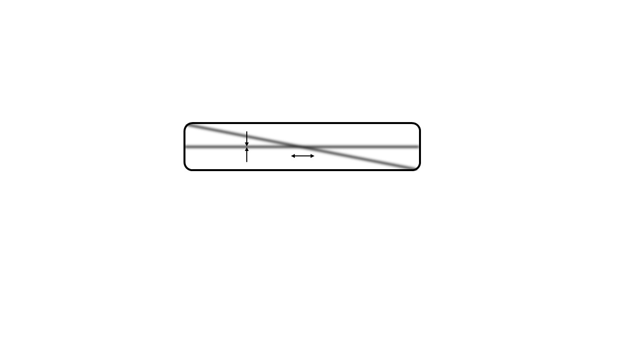
The width of the line might be reduced. However, the visual contrast of the moiré patterns depends on the opening ratio. Maximum contrast of moiré patterns in coplanar grids with a rectangular profile (lying in the same plane) can be achieved with an aperture ratio of one half [23]. With other opening ratios, the visual contrast decreases, and moiré patterns in grids with low opening ratios (i.e., thin lines) have very low contrast (see Figure 1).
Low-contrast patterns can be equivalently replaced [24], but this requires some special size adjustment. However, as the grid moves, the shifted moiré patterns become noticeable. Therefore, the moiré effect can be observed dynamically even in grids with very low aperture ratios (i.e., in very thin lines).
In this paper, we propose treating the intersection of two lines as a moiré pattern. Moiré detection requires overlapping, followed by filtering. Particularly noticeable moiré patterns appear at large distances, i.e., at low resolution. Averaging effectively reduces resolution.
The intersection itself is uninformative and may depend of particular features of lines. Treating it as a moiré pattern (including a low-pass filter) makes it less dependent on specific characteristics of the line. Simulations in the spatial and spectral domains reveal many similarities between the classic moiré effect, which occurs when multiple lines intersect, and the effect of a single lines intersecting.
Except for simulations, practical examples of measurements in the lab (in fully controllable conditions) and in the field (in unreachable locations) using various lines are provided in Sec. 3.
2. Materials and Methods
According to [1], the period of the moiré patterns TM in coplanar grids is,
where T1 and T2 are the periods of the grids, and α is the angle between them.
In particular, when T1 = T2, the formula is simplified:
And the moiré magnification coefficient is
Note that for the moiré magnification, only the angle is important, not the period, aperture ratio, or line count. For small angles
It means that a small angle between the intersecting lines (a small value in the denominator) can produce a significant magnification. Compare the grid displacement with the displacement of the moiré patterns in Figure 1.
3. Results
3.1. Simulation of Visual Moiré
In simulation, we compare the moiré patterns in vertical grids/lines overlapped with a slanted reference grid/line. The vertical grid/line is displaced. The intersection of two lines is treated as the moiré pattern. When measuring displacement using moiré patterns, it is necessary to filter the overlapped grids/lines, and measure the phase of the pattern, which is proportional to the initial grid/line displacement.
The simulation additionally includes the 2D FFT. The sinusoidal grids with different phases are shown in Figure 2 and Figure 3; the rectangular pulses (duty cycle 0.5 and 0.2) in Figure 4 and Figure 5.
In these examples (rectangular/sinusoidal profile, single/periodic pulse), the displacement of the pattern’s center in the spatial domain is the same for sine and cosine functions. In particular, the displacement is the same for trigonometric and rectangular functions with any aperture ratio, including a single thin line. Thus, we can consider a single moiré pattern. This means that for measurements, we can consider the intersection of two lines as a moiré pattern.
3.2. Measured Moiré Displacement
Consider a single vertical line oscillating horizontally, as shown in Figure 6.
The amplitude of the oscillation was 10 pixels. The position of the moiré pattern was obtained according to the definition (i.e., superimposed and averaged). The tangent of the slant angle of the reference line was 1/5, and correspondingly (because the magnification coefficient is 5), the amplitude of the moiré pattern is 50 pixels.
The position of the intersection (and the moiré pattern, therefore) depends on the position of the oscillating line. The resulting measured displacement is shown in Figure 7.
3.3. Practical Examples of Moiré Measurements Using a Single Line
In this section, we describe measurements taken without attaching a physical grid to the object, because oscillations of a small/thin object could be distorted. The measurements were made using the new approach.
3.3.1. Examples with Known Parameters
a. Flower
Oscillations of plastic flowers were measured under "windy” conditions in the laboratory; the “wind” was produced by an electric fan. The flowers with a stem diameter of 1.5-2 mm were 24-29 cm long, see Figure 8.
In the first test, we provided a constant horizontal airflow and recorded a 1-minute video. The measured displacement is shown in Figure 9(a). A 512-point FFT was applied to it. The averaged power spectrum (based on 4 measurements) is shown in Figure 9(b); it shows a center frequency of individual measurements at the spectral intervals (bins) 224-228, i.e., 6.61 ± 0.06 Hz (0.8%).
In the second test, we arranged a periodical airflow. The fan automatically rotated around the vertical axis to the left and right, as shown in Figure 10. The airflow at the flower's location was effectively “turned on” and “off” according to the fan’s rotation.
The measured oscillations of a flower are shown in Figure 11.
A continuous wavelet transform (with Ricker wavelet) was applied to the signal shown in Figure 11. The result (2D array of CWT coefficients and its cross-section) is shown in Figure 12.
The moments when the air "touches" the flower in Figure 11 correspond to those in Figure 12(b). The average period of fan rotations is 9.1 seconds.
b. Antenna
We measured the vibrations of a telescopic antenna on a car navigation device placed on a printer mounted on a high table (as in [22]). The antenna length was 22 cm, and its diameter varied from 2 mm at the base to 0.5 mm at the top. In this test, the navigation device was turned off, and only its housing served as a support for the antenna, as shown in Figure 13.
The measured oscillations are shown in Figure 14 for printouts of different lengths.
The 512-point FFT of the long printout (1.5 pages) contained less noise and had a sharper peak than the FFT of the short printout (14 lines), as shown in Figure 15.
Two peaks can be clearly observed in the power spectrum Figure 15: the fundamental frequency of supporting table at the 101st spectral bin (6.04 Hz) shown by the solid vertical line across two panels (a) and (b) in Figure 15, and the antenna frequency at 188th bin (10.9 Hz) shown by the dashed line. The previously reported table's frequency was 6.26 Hz [22]. The relative difference of frequency with that measurement is 6.4%.
c. Wires in lab
In this test, steel wires were secured between two tables with clamps. The camera was mounted above the wires, mid-span. A horizontal air flow (perpendicular to the wire) was constant. A diagram of the experimental setup is shown in Figure 16.
According to [17], the fundamental frequency is proportional to the diameter of the wire and inversely proportional to the square root of its length,
Measured frequencies obtained in the FFT and estimated ratios of frequencies are given in Table 1.
The measured frequency ratio for two distances (100 and 200 cm) differs from the calculated value of 1/√2 = 0.71 by 1.9% for a wire diameter of 1 mm and by 6.1% for a diameter of 0.6 mm. The ratio corresponding to two diameters (0.6 and 1 mm) differs from the calculated value of 0.6 by 18.2% at a distance of 100 cm and by 14.7% at a distance of 200 cm. The latter are less accurate, probably because this test used uncalibrated wire.
3.3.2. Examples with Unknown Parameters
Unlike the previous examples, exact parameters were unknown in these tests and could only be estimated indirectly.
a. Street wire
The street was observed from a distance of 30 m. The wire diameter was unknown. Wind speed was approximately 10 m/s. The two wires (one along the street, one across) visually intersected, so a reference line was not required for these illustrative measurements; see Figure 17.
The measured signal and its power spectrum are shown in Figure 18.
The power spectrum exhibits a small but noticeable peak at the 46th spectral bin (0.67 Hz). It should be noted that the measurements were taken without a reference line; instead, the reference was found in the video.
b. High voltage line
The distance between the high-voltage poles was several hundred meters. The height of the wire above the ground at the lowest point (where the measurements were taken) was approximately 10 meters. The diameter of the wire was unknown.
The camera tripod was mounted on a solid base (stone); the camera was pointed vertically upward, as shown in Figure 19. The video recording lasted up to 10 minutes.
Figure 20 shows the averaged power spectra measured over several videos (4096-point FFT) for different weather conditions (no wind and wind speed up to 5 m/s).
In the presence of wind, the center of the first harmonic was located at the 26th spectral bin (0.190 Hz, period 5.25 s), and the center of the second harmonic was at the 52nd spectral bin (0.381 Hz). Without wind, the amplitude of the first harmonic was significantly smaller, and its wider peak was located between the 25th and 26th bins (0.186 Hz), but the second harmonic was not detected.
4. Discussion
We examined thin lines with in-camera images fewer than 7-10 pixels.
It should be noted that printer/antenna vibrations were not detected on a hard cement floor.
The limitations of this method are as follows: the line must be straight. The background must be uniform.
Using an inclined line is possible, whereas for cloned lines [22], only a vertical/horizontal line is suitable.
5. Conclusions
Simulations and tests have shown that the intersection of two lines can be considered a moiré pattern, which has the useful property of the moiré magnification. This approach essentially reduces the effective size of the optical target to the intersection of two thin lines. The laboratory and field measurement examples are provided. In the laboratory, the length measurement accuracy is 2-6%, and the diameter measurement accuracy is 14-18%. In the field, measurements were conducted in a hard-to-reach location. The difference with previous measurements is 6.4%. This ensures that single-line moiré measurements can be performed without a special optical target or complex setup.
Funding
This research received no external funding.
Data Availability Statement
The dataset is available on request from the author (the data are part of an ongoing study).
Conflicts of Interest
The author declares no conflicts of interest.
Abbreviations
The following abbreviations are used in this manuscript:
| FFT | Fast Fourier transform |
| CWT | Continuous wavelet transform |
References
- Amidror, I. The Theory of the Moiré Phenomenon. Volume I: Periodic Layers, 2nd ed.; Springer: London, UK, 2009. [Google Scholar]
- Saveljev, V. The Geometry of the Moiré Effect in One, Two, and Three Dimensions; Cambridge Scholars: Newcastle Upon Tyne, UK, 2022. [Google Scholar]
- Patorski, K.; Kujawinska, M. Handbook of the Moiré Fringe Technique; Elsevier: Amsterdam, The Netherlands, 1993. [Google Scholar]
- Post, D.; Han, B.; Ifju, P. High Sensitivity Moiré: Experimental Analysis for Mechanics and Materials; Springer: New York, USA, 1994. [Google Scholar]
- Khan, A.S.; Wang, X. Strain Measurements and Stress Analysis; Pearson: London, UK, 2000. [Google Scholar]
- Singh, B. P.; Varadan, K.; Chitnis, V. T. Measurement of small angular displacement by a modified moiré technique. Opt. Eng. 1992, 31, 2665–2667. [Google Scholar] [CrossRef]
- Fan, H.; Jian, B.; Xiyun, H. Calibration method for angular measurement of moiré patterns based on template matching. Infrared Laser Eng. 2015, 44, 2825. [Google Scholar]
- Zhang, K.; Sun, H.; Yu, D. DOF enhanced via the multiwavelength method for the moiré fringe-based alignment. Micromachines 2025, 16, 356. [Google Scholar]
- Jiang, W.; Wang, H.; Xie, W.; et al. Lithography alignment techniques based on moiré fringe. Photonics 2023, 10, 351. [Google Scholar] [CrossRef]
- Cheng, W.; Chen, Y.; Zhang, Q.; et al. Spatial and temporal distributions of atmospheric refractive-index structure parameter measured by moiré deflectometry. Opt. Commun. 2024, 550, 129966. [Google Scholar] [CrossRef]
- Karny, Z.; Kafri, O. Refractive-index measurements by moiré deflectometry. Appl. Opt. 1982, 21, 3326–3328. [Google Scholar] [CrossRef] [PubMed]
- Chen, X.; Chang, C.-C.; Xiang, J.; et al. An optical crack growth sensor using the digital sampling moiré method. Sensors 2018, 18, 3466. [Google Scholar] [CrossRef] [PubMed]
- Ratnam, M.M.; Ooi, B.Y.; Yen, K.S. Novel moiré-based crack monitoring system with smartphone interface and cloud processing. Struct. Control Health Monit. 2019, 26, e2420. [Google Scholar] [CrossRef]
- Moazzam, A.A.; Ghoshroy, A.; Güney, D.Ö. Remote sensing of seismic signals via enhanced moiré-based apparatus integrated with active convolved illumination. Remote Sens. 2025, 17, 2032. [Google Scholar] [CrossRef]
- Hutley, M.C.; Hunt, R.; Stevens, R.F.; Savander, P. Moiré magnifier. Pure Appl. Opt. Part A 1994, 3(2), 133–142. [Google Scholar] [CrossRef]
- Kamal, H.; Volkel, H.; Alda, J. Properties of moiré magnifiers. Opt. Eng. 1998, 37, 3007–3014. [Google Scholar] [CrossRef]
- Saveljev, V.; Son, J.-Y.; Lee, H.; Heo, G. Non-contact measurement of vibrations using deferred moiré patterns. Adv. Mech. Eng. 2022, 15(4), 1–11. [Google Scholar] [CrossRef]
- Yadil, M.; Morimoto, Y.; Ueki, M.; et al. In-plane vibration detection using sampling moiré method. J. Phys. Photonics 2021, 3, 024005. [Google Scholar] [CrossRef]
- Wang, Q.; Ri, S. Sampling moiré method for full-field deformation measurement: a brief review. Theor. Appl. Mech. Lett. 2022, 12(1), 100327. [Google Scholar] [CrossRef]
- Chen, R.; Zhang, C.H.; Shi, W.; Xie, H. 3D sampling moiré measurement for shape and deformation based on the binocular vision. Opt. Laser Technol. 2023, 162, 109666. [Google Scholar] [CrossRef]
- Saveljev, V. Various Grids in Moiré Measurements. Metrology 2024, 4, 619–639. [Google Scholar] [CrossRef]
- Saveljev, V.; Heo, G. Moiré effect without a multiline grid preserving the phase of a physical image fragment containing a single line. JOSA-A 2026, 43(3), 554–562. [Google Scholar] [CrossRef] [PubMed]
- Saveljev, V.; Kim, S.-K.; Lee, H.; Kim, H.-W.; Lee, B. Maximum and minimum amplitudes of the moiré patterns in one- and two-dimensional binary gratings in relation to the opening ratio. Opt. Express 2016, 24(3), 2905–2918. [Google Scholar] [CrossRef] [PubMed]
- Saveljev, V.; Kim, S.-K. Simulation of low contrast moiré effect in 3D displays. Proc. 12th International Meeting on Information Display (IMID), Daegu, Korea, 2012; pp. 136–137. [Google Scholar]
Figure 1.
(a) Overlapped grids with a low opening ratio (slant angle 100). (b) The same, but vertical grid is moved 5 pixels right.
Figure 1.
(a) Overlapped grids with a low opening ratio (slant angle 100). (b) The same, but vertical grid is moved 5 pixels right.

Figure 2.
Sinusoidal grids, grid1 is symmetric (initial phase as cosine, i.e., 0).

Figure 3.
Sinusoidal grids, grid1 is shifted (phase = π/2).

Figure 4.
Rectangular grid (phase of grid1 = phase of cosine). Layout as in Figures 2,3: grids in rows 1 and 2; overlap and moiré in rows 3 and 4.
Figure 4.
Rectangular grid (phase of grid1 = phase of cosine). Layout as in Figures 2,3: grids in rows 1 and 2; overlap and moiré in rows 3 and 4.

Figure 5.
Shifted rectangular grid. (Phase of grid1 = phase of sine.) Layout as in Figures 2,3.

Figure 6.
(a) Slanted reference line and single oscillating vertical line at two moments of time. (b) Moiré pattern (after Gaussian filter).
Figure 6.
(a) Slanted reference line and single oscillating vertical line at two moments of time. (b) Moiré pattern (after Gaussian filter).

Figure 7.
Measured displacement of moiré pattern in the intersection of two lines.

Figure 8.
Plastic flowers; measurement regions/areas (rectangles) and reference lines (dashed).

Figure 9.
Signal and power spectrum of flower oscillations.

Figure 10.
Layout of the test with a rotating fan (top view).

Figure 11.
Oscillations of a flower under periodical airflow.

Figure 12.
CWT and its horizontal cross-section.

Figure 13.
(a) Layout of antenna test. (b) Measurement region (rounded rectangle) and reference line (dashed line) in the camera frame.
Figure 13.
(a) Layout of antenna test. (b) Measurement region (rounded rectangle) and reference line (dashed line) in the camera frame.

Figure 14.
Measured oscillations of antenna in two printouts: (a) 14 lines, (b) 1.5 pages.

Figure 15.
Power spectrum of printout: (a) 14 lines, (b) 1.5 pages.

Figure 16.
(a) Layout of the wire test and (b) measurement region in the camera image.

Figure 17.
Layout of visually intersected wires including measurement region.

Figure 18.
Measured deflection and its spectrum.

Figure 19.
(a) Layout of measurements, (b) measurement region in the camera image.

Figure 20.
Spectrum of measured wire vibrations with and without wind.


Table 1.
Measured frequencies and calculated/measured ratios to expected values.
| Wire dimensions | Measured frequency, Hz | Ratio of frequencies | ||||||
|---|---|---|---|---|---|---|---|---|
| Diameter, mm | Length, cm | Expected ~1/√L | Expected ~D | |||||
| Calc. | Meas. | Diff. | Calc. | Meas. | Diff. | |||
| 0.6 | 100 | 3.40 | 0.6 | 0.73 | 18.2% | |||
| 0.6 | 200 | 2.26 | 0.71 | 0.66 | 6.1% | 0.6 | 0.70 | 14.7% |
| 1 | 100 | 4.63 | ||||||
| 1 | 200 | 3.21 | 0.71 | 0.69 | 1.9% | |||
Disclaimer/Publisher’s Note: The statements, opinions and data contained in all publications are solely those of the individual author(s) and contributor(s) and not of MDPI and/or the editor(s). MDPI and/or the editor(s) disclaim responsibility for any injury to people or property resulting from any ideas, methods, instructions or products referred to in the content. |
© 2026 by the authors. Licensee MDPI, Basel, Switzerland. This article is an open access article distributed under the terms and conditions of the Creative Commons Attribution (CC BY) license (http://creativecommons.org/licenses/by/4.0/).
Copyright: This open access article is published under a Creative Commons CC BY 4.0 license, which permit the free download, distribution, and reuse, provided that the author and preprint are cited in any reuse.


