Submitted:
02 April 2026
Posted:
07 April 2026
You are already at the latest version
Abstract
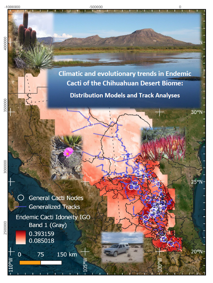
North America´s largest semi-arid lands form the Chihuahuan Desert Biome, which had fluctuated between Interglacial and Glacial conditions for eight million years. Cacti prob-ably came from South America after substantial distancing from Africa, and pollen fossils reveal their arrival in Mexico some 51.6 Ma. We have examined distributions of 119 strict-ly endemics (36.17 % of overall 329 species) and model 75 species represented in well de-fined and relatively large disjunct area groups. We modeled Species Distribution Models (SDMs) using MAXENT algorithms for present and past climates for the region, following our detailed models on climate after Sánchez-Santillán and García detailed numerical methods and Co-Kriging tools. Scotese, Van Devender, Betancourt, and Roy-Priyadarsi were utilized for modelling the glacial part. A total of 4030 registers were sampled from the Central America and North America Cacti Database (UNAM), a comprehensive set of hard information from 68 herbaria and containing over 62,000 vouchers. Registers com-prised 3719 modelable species´ specimens. Track and node analyses were applied using PANBIOTRACKS. We identified the colonization patterns and general evolutionary trends for the species. We modeled detailed combined layers of idoneity and overlap them to tracks and nodes in order to detect biogeographic trends and patterns.
Keywords:
climate change
; Interglacial-Glacial-Oscillation
; biogeography
; track and node analyses
; Cactaceae
1. Introduction
The Chihuahuan Desert Biome (CDB) is a major ecosystem assemblage fluctuating between Interglacial (IG) and Glacial (G) phases in a present–day Glaciation Era [1,2,3]. It was established primarily over the last 8 Ma after the gradual closure of the Central American oceanic bridge [1,4,5]. The continent experienced pertinent climate changes through alterations of the warm water oceanic currents, slowing the intake of cold waters from the Antarctic into the Caribbean Sea [1,5]. This happened after regional orogenies and after new seafloors created by expansionary tectonics, where the hydrosphere can be further held [6,7], highly correlated with important geological proxies [8,9,10] and paleomagnetic evidence [6]. Some large orogenies followed up, as we will see with Laramidia, that correlate with uplifted parts of the Central American Archipelago and several mountains [1,3,5]. A significant process was the increase of humidity towards the equator and the transition of arid and semiarid bands toward the north, establishing mid–latitude arid regions [5]. Few studies delve into reconstructions of present and past climates [8,9], while none had covered track analyses for its cacti. Colonization patterns are explored along with them in correlation to best known phylogenies. Most climatologists accept that we live in an Ice Age [2,3,5], accepted by most serious climatologists, fed by atmospheric dilution and Milankovitch cycles. The iteration, which we call IGO (Glacial–Interglacial Oscillation), has seen 87 cycles, and create climate changes that in combination with soil use, and grazing, are among the drivers of cacti diversity, distribution, and evolution in the CDB [1,11,12]. Cactaceae is an amazing family containing over 1470 species, with at least 800 occuring in Mexico and the Southern USA [12]. The CDB holds over 300 species and has high levels of endemicity [13,14,15,16]. We have fossil pollen in Central Mexico dating back 16 – 51.6 Ma [17], with animals the likely agent for their arrival, allegedly from South America [18] & Appendix A.1. Since then, they moved north and west and reached the CDB some 16–20 Ma, after the rise of the Sierra Madre Oriental (SMO), which completed the rain shadow from Atlantic sources. We modeled the Species Distribution Models (SDMs) using MAXENT algorithms for the IGO and studied 75 modelable species that occur strictly inside the biome, and have enough localities, area coverage, or enough separation between groups of sites. Extremely clogged species resembling a single locality, or species with fewer than 4 sites, were not modeled but were used for richness and general perspectives. IG model came from the application of Sánchez–Santillán and García methods [19,20], while Scotese's works [21], and particular proxies from Roy–Priyadarsi [8,9,10], and clues from packrat middens [22,23,24,25], were used for selection of climatic influence zones and G modelling. Megafauna and human activities have had mostly unexplorable effects over cacti in the biome. Track analyses encompass the calculation of Croizat–inspired patterns that represent ancient biotas, involving evolutionary processes in space, time, and form [26]. Those patterns comprise the graphical integration of biodiversity into identifiable lines and points, tracks and nodes, that show estimated patterns of evolution, which were later compared with Halffter´s Cenocrons [27,28]. These explorations include the cladistic content of biology per region and were incorporated into clear methodologies that improved tests by incorporating mathematical models and digital algorithms [29]; as such, we use in this research [30]. We anticipate that the SDMs will highlight areas with the highest idoneities within the phases of the IGO, revealing potential changes in direction, area drift, size, or areal change. We also suggest that they will reveal the general colonization patterns and will moderately fit with the track and node analyses.
1.1. Objectives
Deepen into the study of the evolutionary and biogeographic patterns of endemic cacti to contribute to the general knowledge of their evolution in space, form and time, by distribution models and track analyses.
- Model the SDMs for the glacial and the interglacial phases of the IGO
- Explore the ancient biotas through track analyses: general and individual tracks & nodes
- Search for a profound understanding of the colonization and dispersal–vicariance within the IGO
1.2. Study Area
The Chihuahuan Desert Biome comprises numerous ecosystems, ranging from extreme arid zones to subhumid montane pine and fir forests [22,24,25] in its mountains. Its origin comes from the closure of the Central American sea bridge [1,4,5] and planetary expansive processes [6,7]. It is part of the North American Tectonic Plate, and was covered by deep waters for some thousands of Ma, before the water moved to new oceanic basins [6]. Reef evidence points toward ancient coastal environments [7]. The movement of the Laramidian sea also caused the Laramidian orogeny through isostatic equilibria and the decrease of the curvature angle of the planet's surface. The lower parts broke open, and the upper parts collapsed toward each other, generating gigantic compression forces that gave rise to its younger mountain range (SMO), which effectively isolated the region from the Gulf of Mexico, creating a much stronger rain shadow [10]. The Sierra Madre Occidental (SMOCC) and the Transmexican Volcanic Belt (TMVB) were already stopping humidity from the Pacific Ocean [8,9,10]. Those two mountain chains were not very different from the present, but the SMO rose mainly after the Chicxulub Impact Crater and the antipode Deccan Traps. During some 50 Ma, volcanic and tectonic activity continued, though plummeting in force [6,7]. Upper parts saw eruptive events and lower parts permeated by magmatic dykes. This topographic complex was uplifted over 3000 m from its original conformation while the water was emptied. The last 18 – 8 Ma saw the closure of the bridge, increased aridification and the establishment of the IGO. Several regionalizations had been proposed.The most natural had been obtained after endemic cacti (see Figure 13.1 in [16]), in which a Main, an East, and a Meridional Subprovinces are recognized. Sierra Transversal de Parras (STP) also divides the CDB roughly into a northern and a southern area. The CDB is now the largest desert environment in North America and the largest temperate desert in Mexico, covering an area of over 508,000 Km2 from the central Mexican plateau and the Queretaro–Hidalgo central valleys, up to the southern region of Texas, New Mexico, and even the tip of Arizona [13,14,31,32]. It traverses 11 Mexican states and goes from higher elevations in the south, toward lower elevations in most parts of the north. We shall understand that most of the recent evolution of the biome as a desertic complex occurred within the IGO [10,32]. That topography has changed little in the last 30 Ma, making cycles of colder and warmer climatic conditions a major driver of the species' evolution on a stable topography. Some 3500 plant species have been described so far, and a wide variety of microfauna and medium-sized fauna survived the arrival of humans some 23.5 Ka.
It was also affected by a major asteroid hit that impacted the northernmost area some 49 ka, and several reiterative fluctuations like the 12.7 ka Younger Dryas and abundant Heinrich events, making cold return along the IGO [33,34]. Climate oscillations, drifting from the G to the IG phases, saw changes up to 8°C, and a much wetter conditions for northern lands during the G, where a large amount of rain descends from the North America directly into the CDB, turning south while colliding with the massive ice shields and the Rocky Mountains under lower and cooler atmosphere´ conditions [4,10,32,34]. The CDB has few permanent rivers and a dozen of glacial lakes, mostly dried during the IGs. Canyons and river basins seem to be related to cacti dispersal and protection, making for IGO´s Refugia.
2. Materials and Methods
2.1. Climatological Layers & Species Distribution Models
The CDB has been regarded as a xerophytic complex of ecosystems that exists inside a substantial rain shadow created by the massive mountains of SMOCC, SMO, and TMVB [10,35,36]. Nowadays, it is considered a Biogeographical Province, after regionalization studies by Morrone and colleagues [28,37]. There are few climatological studies, and most charts were advanced by the mid–1970s by people in the INEGI (Appendix A.3 & SM). To understand more deeply the correlations of the plants, particularly cacti, within the CDB, we needed a solid base. One that does not have the low resolution of the Bioclimatic variables available online, such as Bioclim and Worldclim, obtained mostly from recent satellite information that include serious biases after the present–day thermal peak, a normal pattern along paleoclimatological studies, which might include a minor contribution from anthropogenic sources. A comprehensive Numerical Database was built after methods of Mexican Climatology pioneers Enriqueta García [19] and Norma Sánchez–Santillán [20], which deeply explored around 50,000 selected entries from 60 usable stations within the region, during 1981–2010 (National Meteorological Service, Appendix A.3 & SM). The complex models and their equations are to the subject of a forthcoming contribution and inspired several works, from which we just use the main layers obtained by Co–Kriging tools using elevation after a merged DEM from 39 INEGI´ DEM sources, as the main predictor for the interpolations. Every digital layer in the project was plotted within an hexaquadratic area that increases by 5 % the area toward the borders at all sides, which assures that the complete CDB area is effectively included. Layers were clipped by this increased extension. Information was worked in MS Excel, R, and QGIS / SIG (3.28.3–Firenze). Paleobotanical reconstructions and geological proxies explored by Van Devender [24,25], Betancourt [22] and Roy–Priyadarsi [8,9,10] allowed a numerical transformation and further precise Co–Kriging. These allow climatic regionalization into influence zones, and P/T (water availability) and thermal gradients were applied to obtain the best approximation to the reality of the G condition. The gradients , representing thermal change every 100 m, cross the climatic influence areas by their major axis and are directly related to the precipitation change through the P/T index, by the following formula (1):
Where: P´ = Precipitation at the locality, P = Precipitation average for stations,
T = average mean temperature for the stations, and
T´ = mean temperature calculated for the locality
Gradients were directly applied to obtain thermal anomalies at the localities inside each zone and Formula 1 revealed water availability and precipitation best approximations. A total of 2015 localities were modeled following the gradients for each zone, and 11 anomalies were predicted: Mean normal temperatures, maximum mean temperatures, maximum extreme temperatures, mean minimum temperatures, extreme daily minimum temperatures, year normal precipitation, month normal precipitation, and days with: Fog, hail, storm, and rain. Numerical models are shared in summary in SM, (climatic types for each specimen correspond to keys in Appendix A.4). Co–Kriging detailed or fine interpolated layers were created: Seven for the IG part, and five for the G part (Appendix A.3 & SM). This is a powerful and comprehensive exploration of real climatologies as best one could assess, and allowed us to explore correlation trends within the species, and much more importantly, model the IGO SDMs with high precision and correspondence to understand changes within the phases. Extensive revisions of this fine models had allowed research on quantitative Refugia, environmental correlations, rarity and climatological specialization in turn for other works, and hereby, the exploration of the correspondence between idoneities and track analyses for the strictly endemic cacti in the CDB. Co–Kriging searching tools were limited to 1° geographic with square dimensions of 0.01° geographic and 30 aggregations. Several available information layers were used to construct the figures of this work, including INEGI city and road shapefiles, USA/USGS/NOAA shapefiles, and a visualization layer fitting available in QGIS, such as Google Terrain, Google Satellite, and World Countries Borderlines. Geographical maps and the Coordinate Reference System (CRS) of the project were projected after WGS84 ellipsoid (World Geodetic System 1984, EPSG:4326. Ellipsoid: major semiax = 6378137.0 m, flattening = 1/298.257223563). Illustrative maps contain both the geographical degree system and the lines for the Universal Transverse Mercator (UTM). ASCII files used for MAXENT SDMs for the IGO are shared in the SM, additional materials are available by request. MAXENT (Maximum Entropy Modeling Alforithm), developed by the Center for Biodiversity and Conservation at the American Museum of Natural History (AMNH) under the guidance of Steven Phillips and other AMNH´ colleagues [Appendix A.2], consist of a machine–learning algorithm that allows the iteration of a species known points through a distribution area for the selection of environmental features within disposable raster layers (Appendix A.3 & SM), to create suitability or idoneity maps where the species might thrive best (https://biodiversityinformatics.amnh.org/open_source/maxent/). We used routines developed by Joshua Banta and colleagues (University of Texas at Tyler; https://sites.google.com/site/thebantalab/home) in an R script to initially test for the most adequate models to use in each case, the number of replicates, and the regularization multipliers (Appendix B.1 & SM). Cross–validation and particular determined models–regularization multipliers were used with 10,000 background points for modeling 75 species in the IG and G phases. In each case, the relevant climatic layers were used to plot idoneities, and SM. The SDMs were later used to create combined idoneity maps for the IG, the G, and the IGO. They were also tested, containing just the climatic specialists. Raster Calculator of QGIS was used to perform the combinations and particular analyses of the information. 75 SDMs for the IGO were compared in order to determine general trends in size, position and drift over time. MAXENT were used due to their robustness in handling presence-only data and their widespread application in biogeographical research, we prefer such scope over alternative models because it has proved strong value and good results beyond particular or ecological-niche-oriented algorithms that are focused on short term climatological variations. Cacti are long lived plants with decades to hundreds of years life spans, which also provide confidence on using our mean variables for the IG and G phases of the IGO. The R routine procedures allowed the identification of the most appropriate model configurations prior to final implementation (SM table). Although we do not aim to compare alternative modeling algorithms, particular care was taken to ensure that model complexity and performance were adequately controlled to minimize overfitting and maximize interpretability of long-term and wide-scale climatic suitability patterns, that under our high quality data approach probabilities.
2.2. Track Analyses and Evolutionary Correlations
Analyses tools were used to create intersections of localities (2015) and specimen registers (3719), filtering the original 4070 specimens and focusing in the 3719 specimens from the modelable species with corroborated georreferences. The intersections allow the creation of SIG–based occurrence tables and plots that reveal the structure of alpha diversity and suggest a noticeable beta diversity, as determined in several documents to date [11]. Endemism is evaluated on the possibility that the species were endemic to one, two or the three subprovinces sensu Hernández & Gómez–Hinostrosa [16], whereas a larger occurrence makes for a lower Endemism value. Track analyses can be mapped as free-hand made integrations or by using digital algorithms. Tests were performed using Parsimony Analysis of Endemism, but the matrices were low in occurrences for obtaining a clear perspective on the tracks and nodes. Thus, we decided to use a new integrative program called PANBIOTRACKS, designed by Carlos Castillo and already tested for several taxa [30]. The program involves R algorithms that find the nearest correlations among individual tracks of a species in order to create internal generalized tracks, by comparing the lengths and the angles in which each individual track appears over the space. It has also subroutines that are able to correlate the highest densities of tracks approaching each other to deduce main nodes. The tracks and nodes represent the ancient biotas suggested by their present–day remains or manifestations. We studied general tracks and nodes, and make selections of species that possess wide and limited forms of dispersal to have a set of different comparable graphic results that could explain particular biological trends. Cacti, specially Opuntioideae but also Cacteae, show a noticeable level of horizontal translocation of loci, by means of fertile hybridization and molecular vectors. This is probably the case for numerous groups of plants and almost every simple life form in the planet, which might oppose traditional strict views of dichotomic evolutionary trends and suggest nets of life for plants, rather than simple dichotomous trees. Our best try was to integrate the best-resolved phylogenies (Appendix A.1), and the tracks for the known chronologies to compare the species with particular and general tracks and nodes. Matrices were also built after the occurrence of all tracks and nodes over a ¼ geographical degree grid, which might also be informative of the number of overlappings among the individual and generalized patterns. Finally, sizes and positions of the overall idoneities for each of the 75 modelable species were compared by general overlapping of the SDMs in order to detect the trends of evolutionary change, thus being able to suggest lines of vicariance, dispersal and reduction within their potential distributions. We consider that doing so is our best guess, since independent and individual events of vicariance or dispersal are almost untracktable. Species distributions contracting the most are thought to be a signal of potential extinction threat within the IGO.
2.3. Hypotheses Testing
We propose that overlapping the overall idoneities of species with the overall tracks and nodes for them will reveal substantial coincidences between them. We also suppose that widely distributed species will have long reach and wide tracks, and that limited distributed species will have limited tracks and much more complex ramifications and nodes than the widely distributed ones. We advanced overlappings of the idoneities, tracks and nodes to test this ideas graphically, where analyses pinpoint toward colonization of the environments allegedly coming from its South–Eastern tip. Chronologies were included.
3. Results and Discussions
A total of 119 endemic cacti species were surveyed, and 4503 specimens were revised regarding taxonomic status clarity and geopositioning precision, from which 17.4 % were eliminated after gaps. Thus, 3719 specimens corresponding to 2015 confirmed localities were carefully assessed, and focus was given to 75 species, which occur at least over 85 % of the time inside the CDB, and 44 species were represented as points within the GIS, and are not useful for modeling or track analyses. These species happen on 126 ¼° squares within the CDB. We recognized nine chronologically integrated clades from the eight best–resolved phylogenies (Appendix A.1) and superimposed their SDMs for the IGO (Figure 1a), identifying 37 potential dispersal events, 59 potential vicariance events, and up to 22 potential extinction risks. These numbers are not close ones; instead, they are trends or drifts deduced from changes in idoneity in the IGO models. Most common species are Mammillaria formosa, Echinocereus pentalophus, Ferocactus pilosus, Opuntia microdasys, Ferocactus hamatacanthus, Ariocarpus retusus, Mammillaria compressa, Echinocereus enneacanthus, and Thelocactus bicolor. A total of 44 microareal non–modelable species make 119 endemics.
3.1. Species Distribution Models
Endemism is naturally correlated with the greater area of the Main Subprovince, covering most of the CDB. Nevertheless, it is complemented with the Meridional Subprovince (Table 1). Meridional Subprovince attains noticeable occurrences of Lophophora diffusa, Opuntia pachyrrhiza, and Turbinicarpus pseudomacrochele, despite that they could be found in fewer localities otherwise. We present each species idoneities on the SDMs in the SM, where plots and information on them is made accessible. Visual general comparisons allowed the detection of the patterns pinpointed before, which are also summarized in Table 1, where values from 0–1 concerning endemism and climatic specialization are shown. A cumulative species idoneity map for the IGO is presented in Figure 1a, whereas Figure 1b and 1c show the idoneities for species preferring temperate climates (IG) and semi–arid climates (G) for wich we have complete detailed matrices by localities (SM, Appendixes B.3 & B.4). The table summarize main phase for wider distributions for the species, and contains the general trend observed in the plots, followed by the potential change trends for the distributions, and the processes being suggested by those changes. We think that it is impossible to track every evolutionary process and it is likely that such idea will remain impossible forever since we have very small information of just present–day survivors of a long evolutionary history. So we do not intend to reconstruct particular vicariant or dispersal events, but rather to focus on what the change in the distributions could actually tell us for the last part of the IGO. We present the idoneities also in a chronological order looking for clues on their fitness over time and colonization sources. Composite Figure 2 reveals the patterns of colonization and radiation in the CDB, and is in agreement with the track analyses and evolutionary phylogenetic correlations that we present. Idoneities for Age Clades defined after the best-resolved phylogenies (SM) are clipped by the known Areas of Occupancies. A potential extinction gap is easily identified in Figure 1a, perhaps after increasing intensity of the glacial phases aridity or extreme values.
Dispersal methods can vary from the hyperdispersal of some Opuntia to the scarcity and specific correlations of small globose species, like Aztekium, Obregonia, Ariocarpus, and many Coryphantha and Mammillaria. Larger species often rely deeply on fruit succulence for far–distance dispersal by extinct megafauna, present–day mid–fauna, and have even been modeled after human uses and distinct traditions, causing range distribution alteration [18,31,32]. Some cacti had been definitively introduced by humans from one region to another, while most strictly endemics fall far from this trend. It is possible that distributions of Opuntia microdasys and O. rufida, Lophophora williamsii, and even Neobuxbaumia, as well as some Echinocereus and Ferocactus pilosus, might have been altered by human management after their common use in diet or construction. The first three species are outstanding in their responses to human–induced changes and were surely manipulated since the earliest arrival of ancient peoples. A Maximal Idoneity Area (MAXI) fulfills several needs to quantify the abundance of endemic cacti through the IGO and the overlapping of these areal calculations with track and node analyses, with 19 species on a 75% probavbility occurrence (Dotted area, Figures). A general 0.27 idoneity threshold was used for the general IGO cacti idoneity after analyses of the natural breaks in the histogram of the point cloud. This was found to represent the presence of at least 19 species of species found to overlap with 90 % of the generalized tracks, 82 % of overall nodes, and represents 72.43 % of all revised specimens (3719 vouchers) in just 24.7 % of Hernández & Gómez–Hinostrosa Regionalization [16], or just 15.7 % of the hexaquadratic area used for this study. This means that about 84% of the CDB area has low richness compared to the latter, which contains most biodiversity, highlighting the evolutionary connections.
3.2. Track Analyses and Evolutionary Correlations
Track and nodes´ studies focus on searching tracks joining specific localities for species, ordered in a parsimonious way. Those tracks are used to obtain internal generalized tracks for endemic cacti species in general, while we also performed track and node analyses for species with widespread and limited dispersal. We see these tracks and nodes (Figure 3 and Figure 4) as a window into species interconnectivity and a potential explanation of their evolutionary trends, when the orientation is inferred from changes in the predicted idoneities for the IGO. The general orientation of all the tracks is SE–NW, and several tracks and nodes point into the recognized SE-NW direction of the potential colonization, which could be appreciated in Figures and was counted through the 136 ¼° squares with cacti, confirming the following statements (Table 2). We find major tracks going from the Meztitlán and Tolantongo Gorges, in connection with the Mezquital Valley, communicating with central SLP valleys [32]. The general tracks (Figure 3) point toward a dense interaction with major gorges and valleys of the Zimapán–Tolimán–Cadereyta region, and into the plains of SLP. El Huizache and Mier y Noriega, widely known for their incomparable richness and diversity, are quite in the middle of several tracks and nodes, and they correlate directly with several eastern Tamaulipecan valleys and mountains, both in the Main and in the Eastern Subprovinces. Seemingly, tracks go north by the side of the SMO and through the valleys between the middle SLP ranges and Real de Catorce range. The eastern division rises up toward the STP and intermixes thoroughly with SMO, while the western patterns go directly upon the Mazapil–Saltillo region, crossing the STP, creating two parallel tracks toward the southern and northern slopes of the STP. A significant track crosses Coahuila and connects several mountain ranges and dry valleys into interesting routes for dispersal and even for some more vicariance. Sierra La Paila and the Valley of Cuatro Ciénegas join some other valleys, such as El Hundido and Anteojo, in a complicated road for cacti toward the northern areas. El Burro and el Nido ranges, Maderas del Carmen, and the Big Bend National Park region highlight the Northern areas. Some tracks follow northwest near the Rio Grande basin, while a minor one diverges toward the Bolsón de Mapimí through the southern edge of Laguna de Mayrán basin, a large glacial lake that mostly dries up during the IGs. Analyses for species with high reaches (Figure 2 and Figure 4a), those that can travel in the stomach of mid fauna or proxies for the extinct megafauna [18], and that sometimes even disperse through segments – like Opuntia – look straightforward and far reaching, simple and not very dichotomized. In contrast, tracks for scarcely propagated species depending on minor fauna, wind, and water upon local dispersal, are tremendously intricate, not far–reaching, and often intermingled (Figure 4b). These tracks extend into mountains and mountain valleys thoroughly, and nodes for such species rise to 45, while far–reaching species have just six nodes. We propose that a closer look at the individual tracks might reveal something for future studies, and understand that what we are looking at is a complex intermix of dispersal and vicariant events over the IGO, which is roughly explored so far.
Climatologically, we notice four relevant effects within the IGO: SMO Oceanic – corresponds to climates moderated by a reasonable Atlantic influence [8,9,33] through north winds and occasional humid intromissions, Northern Areas – mostly dry during the IGs, they see the most significant changes on humidity and water availability in comparison between the IG and the G phases–conditions, SMO SMOCC – High Pressures over the dry part of the Sierras is usually quite stable even in the G phases, but always preserve somewhat wet and cool environments on the high parts, and South Highlands – elevated mountains and volcanoes toward the Meridional Subprovince are well known for their temperate woods, mesic and even cool environments throughout the IGO. A numerical transformation (0–1) from lower to higher effects is provided in Table 2, where the mean thermal and precipitation changes (x times–folds) from the current IG conditions toward the Mean G conditions can be appreciated. Means refer to species–averaged anomalies, while extreme temperatures are explored in their graphical form in the climatological and SDMs sections. Significant climatic changes override the whole biome, with a 4–7–fold increase in humidity from the north, since massive ice fields and the Rocky Mountains – under a thinner, cooler, and relatively drier general atmosphere – make winds turn southward directly into Mexico during the G phases. However most cacti receive smaller changes on P/T as seen in Table 2. The Northern Areas receive thus the significant climate change in relation with their IG well known aridity, but climatic and vegetation floors change widely, between 6 and 12° C and up to 5 times the P/T indexes we will explore further. Most tracks and nodes occur in low–change areas, as large water availability may involve significant transformations of vegetation communities, potentially affecting climate–vulnerable cacti. As we will see later, several species tolerate lower temperatures and even increased humidity without major problems, and many others even prefer those conditions in mesic–temperate lands during the IG phases. In contrast, some other species prefer aridity and benefit from particular mountain shadows and southern protection from the humid north during the glacial periods. We suggest dispersal is critical for widely propagated species. Still, they are the least among strict endemics of the CDB, whereas evolutionary trends indicating that the species mainly came from the SE tip of the biome are clear. We think that plant rarity and high climatic specialization speak to the dominance of allopatric speciation and align with track analyses.
The eight best phylogenies (Appendix A.1) probably explain the associations among cacti, and were also used to group them by age–clades as best as possible. As seen in the composite Figure 2, SDMs of specific species are congruent with phylogenetic expectations and pinpoint nine cacti minimal–age clades for the CDB, based on the best-resolved phylogenies to date. Tracks and nodes corroborate the patterns shown in the figures and reveal additional correlations within the phylogenetic clades. Cacti arrived mainly or uniquely from the SE tip, and clades I and II rapidly colonized most of the central and northern areas, first passing through the Meridional Subprovince. Astrophytum and Sclerocactus were shortly followed by Opuntioids, perhaps colonizing environments and allopathically creating species some 30 – 16 Ma. Even Coahuila and the central–north diverse regions were early colonized and populated, although it seems that species remained in big valleys and plains, to later evolve into the thin ravines and valleys in the buttresses of SMO and the transversal ranges. Clades III to V evolved even some eight Ma, or somewhat later, coinciding with the effective climatic formation of the CDB´s IGO. They include mostly Mammillaria, a broad genus with the most considerable species richness in Cacteae. Many such species, together with Coryphantha, support elevated humidity and often occur among cold– and wet–preferring species. Later, Clades VI and VII developed further into the ravines and isolated plains, colonizing new environments. Clades VIII and IX were the last to evolve and appear to have existed for less than 5 Ma. They primarily include the recently evolved Echinocereeae and small to large species that do not often support freezing temperatures and remain excluded from very high places and northerly lands. However, even among them, we can find species that support extreme cold and humidity. Opuntioideae are the only fossil pollen confirmed so far from the surroundings of the CDB (Ramírez–Arriaga et al. 2017; TCV, 16 Ma), but other samples are known from southern Oaxaca that exceed 50 Ma [17]. We can be sure that at least Opuntia arrived early, while minimal ages for different branches and specific species are inferred from the molecular clocks, where proxies serve as indicators. There are some interesting manuscripts on the issue, and perhaps Arakaki et al. (2011) and Silva et al. (2018) gave a good look into evolutionary times. However, we adjusted Arakaki´s timelines considering a 34.7 % subestimation derived from the tangible evidence near the CDB and included the adjusted molecular clocks in the species that can be tracked down.
As exposed in the main tracks, and following the SDMs of the clades (Figure 2), there are mostly entrance patterns from the SE tip of the desert and a series of complex dispersal and vicariant events, perhaps counted in the hundreds, that also might have included some extinctions in the relatively recent geological time. SDMs, and their drift and change are extracted by comparing the G and IG best models (SM). We were able to suggest potential states favoring dispersal and vicariance, although the distinct events could not be easily reconstructed or even perceived. We also pinpoint species with a significant risk of extinction within the last IGO cycle, and the present–day species that would receive additional protection after these discoveries. Twenty–two species show a larger ecological niche for the IG conditions, while 17 species have equivalent species distributions in the overall IGO (Table 1). Thirty–six species have a greater distributions during the G phase, highlighting the importance of both phases in the evolution of cacti. Some 37 cases of potential dispersal and 59 of potential vicariance were highlighted for the last transition from G to IG conditions (Table 1). In contrast, they might imply more specific processes on the move. The extinction threats refer to potential risks after substantial reductions in identity areas, not to direct measures as reported by Goettsch et al. (2015) in their assessment of the conservation status of the family [11]. This does not necessarily imply that the species are currently on the brink of extinction, but it may help improve IUCN Red List evaluations and propose future biome conservation schemes. There are twelve species potentially drifting their distributions toward the center, five toward the center–east, two toward the center–north, three toward the center–south, six toward the center–west, seventeen equally distributed, 10 toward the northwest, five toward the west, and several other intermingled cases. Twenty–two species contracted their suitability areas, 34 species diverged in their distributions, and 16 species remained the same during the last fluctuation. Coryphantha werdermannii, Homalocephala parryi, and Mammillaria moelleriana noticeably expanded their suitability area, probably increasing through this phenomenon into new dispersal events [27]. We suggest that species that contract their SDMs and have limited ways of dispersal could be at most risk. However, that could depend on varied threats and the current state of land use, therefore conservation improvements require much more studies.
3.3. Hypothesis Evaluations
We see that there is actual overlap between general, wide–dispersed, and limited–dispersed species' tracks, with higher idoneities calculated for the IGO. There is also a strong pattern showing that the western side of SMO is the most important idoneity–track superposition, and that is explained after the combined protection effects and the rain shadow provided by this longitudinal range. Its western derivation through the STP divides the CDB into two parts: A northern arid area during the IG and a wet area during the G that limits cacti survival, and a southern area that extends even towards the Eastern and Meridional Subprovinces, where larger idoneities are found, and Refugia are likely for the IGO. Widely distributed species indeed met wide and long tracks, and limited species also had limited, very complex anastomosed and intricate tracks, thus corroborating our hypotheses. The southeastern tip also correlates with what we perceive as the colonization channel for the CDB, through the valleys of Meztitlán, Tolantongo, and Mezquital, which connect the biome with Central Mexican Valleys, TCV, and even the Balsas Basin towards the S–SW.
4. Conclusions
Endemic cacti provide a window for present and past exploration of the CDB and have revealed interesting patterns regarding their distribution (SDMs) and their evolutionary trends. Cacti undoubtedly entered the CDB area through the southeastern tip, probably crossing several central Mexican temperate valleys more than once, and then colonizing the Meztitlán and Tolantongo Gorges, passing to the Mezquital Valley and dispersing all over the SLP valleys towards Tamaulipas to the east, and towards Zacatecas and Coahuila to the north and northwest. Astrophytum, Sclerocactus, and Opuntia dispersed first, while Coryphantha, Mammillaria, and Lophophora probably dispersed and radiated later. It´s even possible that Escobaria, Lophophora, Obregonia, Pelecyphora, and Neolloydia radiated within the very CDB during well–established IGO variable conditions. The same could be said, for younger ages, for Ariocarpus, Epithelantha, Thelocactus, and Turbinicarpus, to a certain extent. The last genera present new taxonomic challenges because they appear polyphyletic. However, horizontal transfers within Cacteae are significant and potentially affect Mammillaria and Coryphantha. Opuntia is the largest genus in Mexico and undoubtedly contains high amounts of horizontal gene transfer via hybridization, virus vectors, and even gardening practices.
However, the strictly endemic species considered here are not widely commercially used, serving mostly as livestock forage, and perhaps are less affected than other utilitarian species. Hundreds of dispersal and vicariant events might had been involved in the evolution of present–day cacti of the CDB, which might likely reveal unexplorable in detail. Still, we can deduce the number of species decreasing their distributions from the last G to the present IG [32]. Around 23 % of the species did not substantially change their suitability during the last episode of IGO, while many others either reduced or increased their potential distributions, perhaps in relation to IGO´s Refugia. Diversity and idoneity is higher in the SMO's central squares of Huizache, Mier y Noriega, and the Tamaulipecan valleys. We also have some rich areas in the Meridional Subprovince, and even around Mazapil´s square, towards Cuatro Ciénegas and the Maderas del Carmen–El Nido–Cañón de Santa Elena–Big Bend areas. Evolutionary patterns concerning the relevance of central SLP valleys, the Tamaulipecan valleys, and the Queretaro–Hidalgo valleys are undebatable. We think that this study pinpointed the general patterns of colonization, vicariance and distribution fluctuation on the correct scenario of IGO effects, and correspond well with a IGO development following the decreasing power of Central America´s oceanic currents and the drift of deserts to higher latitudes. Cacti also experienced gradual change in mobility forms through extinction of mid–fauna and megafauna. They arrived quite early from the south in the stomachs or on the hair and feathers of animals, and later traveled on herbivorous large mammals that eventually became extinct as a combination of human pressures and intense environmental change. Cacti exhibit incredible resilience and persist in fluctuating distributions, serving as a significant element of the CDB´s floristic composition. LGM is suspected to be a good estimation of G conditions, and the present–day climate a nice view of a mean IG. Tracks and nodes widely coincides with the suitability obtained for the endemic cacti through the IGO, because many patterns occur in the MAXI, including generalized tracks and several types of internal correlation nodes, sensu Escalante. About 90 % of total tracks and over 80 % of overall nodes are contained inside this relatively small area, covering around 24 % of CDB´s sensu Hernández (122,000 km2) [16]. It also contains many species that are high climatic specialists. We recognize that water availability is not the only causation factor behind the development of significant drifts in vegetation, thus not neccesarily implying giant grasslands or forest–covered transitions in all parts of the CDB [32,38]. Results show that several G–temperate loving species refuge in mountain tops and protected valleys, with lower temperatures and somewhat moister conditions. Considering cacti distributions and evolution is very important for improving our comprehension of the CDB, and most likely needed for the creation of sound conservation proposals [11,13,14,31]. Tracks clearly follow the mountain´s rain shadow and the highest idoneities and richness in both phases of the IGO. They also show interesting trends toward overlapping species idoneities, that could almost be taken by probabilities after data quality. Their patterns correlate with those found in the SMO [39]. Highly dispersed species show long and more simple tracks, while propagation–limited species are indeed intricate and complex, and much more constricted to ranges and valleys in the Main and Meridional Subprovinces of the Grand Biome. Nodes are informative, but could vary much more than the tracks. We found correlative nodes among main tracks and strongly suggest that the inter–province or inter–region nodes, sensu Morrone, are to be found within the SE tip toward the TMVB and the central valleys of Mexico and the Balsas Depression, and toward the NW tip concerning the Madrean Region relating the CDB to the Sonoran Desert. Although distinct vicariance and dispersal events are almost impossible to explore and understand, being the evidence limited and mostly erased from the face of the Earth other than heritage possibilities, we demonstrate that SDMs can be compared to suggest change patterns along the IGO. We can also measure the overall occurrence of tracks and nodes over space in order to pin–point relevant areas. On an expanding planet, atmospheric dilution is the main driver of aridity and desert growth, favoring arid-adapted species. Cacti surely will have a promising and long-term future in that major trend.
Supplementary Materials
The following supporting information can be downloaded at the website of this paper posted on Preprints.org, Climatic Database, SDMs R routines and Data, MAXENT MODELS IG & G, Climatic Layers IG & G, PANBIOTRACKS LISTS/MATRICES, PANBIOTRACKS´ SHP, DBF AND SHX FILES. Detailed Environmental Database and some Georreferences by request.
Author Contributions
David Brailovsky-Signoret was the primary author and intellectual proposer of the project, he performed conceptualization, data curation, formal analyses, research, methodology, administration, resources, validation and visualization on different aspects of the project, including working on extensive databases, climate modelling, SDMs, biogeographical tests and Geographical Information Systems, including the final development of detailed climatic layers. Héctor Hernández is the principal advisor of the first author and has made a significant contribution to the conceptualization, data curation, formal analysis, funding acquisition, methodology, resources, and supervision of the overall project. Gabriela Castaño-Meneses contributed to various aspects of the methodology, investigation, resources, and formal analyses. Héctor and Gabriela both revised the manuscript, having brought prospective advisory and review & editing. CGPT was used for ordering some tables and for renumbering the citations after Diversity requirements.
Funding
This work and its associated research efforts were supported by a Doctoral Grant from the Secretaría de Ciencia, Humanidades y Tecnología (SECIHTI) of the Government of Mexico, and partially supported by Posgrado en Ciencias Biológicas, National Autonomous University of Mexico (PCB, UNAM). The International Organization for Succulent Plant Studies (IOS) provided us with funds for fieldwork in 2024. All the authors contributed an additional amount to the development of this research and fieldwork expenses. Elia Ramírez-Arriaga provided us with academic and financial support during part of the fieldwork conducted in 2024.
Data Availability Statement
All relevant DATA from this study are shared in the Supplemenary Materials (https://www.mdpi.com/article/doi/s1), detailed Information available by request*.
Acknowledgments
This paper is part of the requirements for obtaining a Doctoral degree at Posgrado en Ciencias Biológicas, UNAM. We thank Posgrado en Ciencias Biológicas (PCB) of the National Autonomous University of Mexico, and SECIHTI, for their support for the doctoral studies and research project. PCB, SECIHTI and IOS granted financing. Thanks to the Institute of Biology and the I. of Geology, UNAM, for their academic support, vehicle ease, and fieldwork assistance. We thank the National Meteorological Service for detailed climatic information. Much thanks to Carlos Gómez-Hinostrosa for laboratory help. Jacinto Treviño Carreón, Paola Sánchez, Daniel Xilote, Elia Ramírez-Arriaga and Camerino Salinas help in the fieldwork. Juan José Morrone, Rolando Bárcenas-Luna and Teresa Terrazas-Salgado shared phylogenetic information and theories. Carlos Castillo, Josh Banta and Norma Sánchez-Santillán gave advice on methodologies. Christopher Scotese and Roy-Priyadarsi gave inspiration on paleoclimatology. James Maxlow shared his works on plate tectonics. We thank Jane Rosenthal for style advice. QGIS was essential. Roberto Bonifaz Alfonso and Miguel Ortega Huerta inspired SIG analyses.
Conflicts of Interest
There are no particular economic or academic interests to declare, and neither any conflicts of interest within the authors in the present work. All materials are provided after scientific communication proposals and are intended to open new perspectives on the evolutionary biology of cacti in the Chihuahuan Desert Biome, which may be applicable for conservation purposes thereafter.
Abbreviations
The following abbreviations are used in this manuscript:
| Ma | Million years / Million years ago |
| MDPI | Multidisciplinary Digital Publishing Institute |
| AMNH | American Museum of Natural History |
| CDB | Chihuahuan Desert Biome |
| CRS | Coordinate Reference System |
| DEM | Digital Elevation Model |
| G | Glacial |
| IG | Interglacial |
| IGO | Interglacial-Glacial Oscillation |
| INEGI | Instituto Nacional de Estadística, Geografía e Informática |
| LGM | Last Glacial Maximum |
| MAXENT | Maximum Entropy Modeling Algortithm |
| NW | North-West |
| SDMs | Species Distribution Models |
| SE | South-East |
| SLP | San Luis Potosí |
| SM | Supplementary Materials |
| SMO | Sierra Madre Oriental |
| SMOCC | Sierra Madre Occidental |
| STP | Sierra Transversal de Parras |
| Tamps | Tamaulipas, Tamaulipecan |
| TCV | Tehuacán-Cuicatlán Valley |
| TMVB | Trans-Mexican Volcanic Belt |
| UTM | Universal Transverse Mercator |
Appendix A
These Appendix contains the main keys for understanding climate types and information also available as independent archives in the Supplementary Materials. It is shared here as a simplification for the readers. R Algorithm Routines used for the selection of the best models for SDMs in the IGO, and the synthesis of the Environmental Matrix are contained in the Supplementary Materials. Particular analyses are described along the text, more detailed data by request.*
Appendix A.1. Most Complete Phylogenetic Reconstructions
[a] Arakaki, M., Christin, P. A., Nyffeler, R., Lendel, A., Eggli, U., Ogburn, R. M., Spriggs, E., Moore, M. J., Edwards, E. J. (2011). Contemporaneous and recent radiations of the world's major succulent plant lineages. Proceedings of the National Academy of Sciences, 108(20): 8379 - 8384. https://doi.org/10.1073/pnas.1100628108
[b] Bárcenas, Rolando T.. (2016). A molecular phylogenetic approach to the systematics of Cylindropuntieae (Opuntioideae, Cactaceae) Cladistics. 32, 4: 351-359. https://doi.org/10.1111/cla.12135
[c] Bárcenas, Rolando T.; Yesson, Chris; Hawkins, Julie A.. (2011). Molecular systematics of the Cactaceae. Cladistics. 27, 5: 470-489. https://doi.org/10.1111/j.1096-0031.2011.00350.x
[d] Guerrero, Pablo C; Majure, Lucas C; Cornejo-Romero, Amelia; Hernández-Hernández, Tania. (2019). Phylogenetic Relationships and Evolutionary Trends in the Cactus Family. Journal of Heredity. 110, 1: 44287. https://doi.org/10.1093/jhered/esy064
[e] Hernandez-Hernandez, T.; Hernandez, H. M.; De-Nova, J. A.; Puente, R.; Eguiarte, L. E.; Magallon, S.. (2011). Phylogenetic relationships and evolution of growth form in Cactaceae (Caryophyllales, Eudicotyledoneae) American Journal of Botany. 98, 1: 44-61. https://doi.org/10.3732/ajb.1000129
[f] Sánchez, Daniel; Vázquez-Benítez, Balbina; Vázquez-Sánchez, Monserrat; Aquino, David; Arias, Salvador. (2022). Phylogenetic relationships in Coryphantha and implications on Pelecyphora and Escobaria (Cacteae, Cactoideae, Cactaceae) PhytoKeys. 188, : 115-165. https://doi.org/10.3897/phytokeys.188.75739
[g] Vázquez-Lobo, Alejandra; Morales, Gisela Aguilar; Arias, Salvador; Golubov, Jordan; Hernández-Hernández, Tania; Mandujano, María C.. (2016). Phylogeny and Biogeographic History of <I>Astrophytum</I> (Cactaceae) Systematic Botany. 40, 4: 1022-1030. https://doi.org/10.1600/036364415X690094
[h] Vázquez-sánchez, Monserrat; Sánchez, Daniel; Terrazas, Teresa; De La Rosa-Tilapa, Alejandro; Arias, Salvador. (2019). Polyphyly of the iconic cactus genus Turbinicarpus (Cactaceae) and its generic circumscription. Botanical Journal of the Linnean Society. 190, 4: 405-420. https://doi.org/10.1093/botlinnean/boz027
[i] Vázquez-Sánchez, Monserrat; Terrazas, Teresa; Arias, Salvador; Ochoterena, Helga. (2013). Molecular phylogeny, origin and taxonomic implications of the tribe Cacteae (Cactaceae) Systematics and Biodiversity. 11, 1: 103-116. https://doi.org/10.1080/14772000.2013.775191
[j] Wilson, J. S., Pitts, J. P. (2012). Identifying Pleistocene refugia in North American cold deserts using phylogeographic analyses and ecological niche modeling of Polistes biglumis (Hymenoptera: Vespidae). Biological Journal of the Linnean Society, 105(3): 515 - 529. https://doi.org/10.1111/j.1095-8312.2011.01812.x
Appendix A.2. MAXENT & SDMs Background-Methodological Bibliography
[a] Phillips, S. J., Anderson, R. P., & Schapire, R. E. Maximum entropy modeling of species geographic distributions. Ecological Modelling, 2006. 190, 3–4: 231–259 https://doi.org/10.1016/j.ecolmodel.2005.03.026
[b] Elith, J., Phillips, S. J., Hastie, T., Dudík, M., Chee, Y. E., & Yates, C. J. A statistical explanation of MaxEnt for ecologists. Diversity and Distributions, 2011. 17, 1: 43–57 https://doi.org/10.1111/j.1472-4642.2010.00725.x
[c] Merow C., Smith M.J., & Silander J.A. A practical guide to MaxEnt for modeling species’ distributions: what it does, and why inputs and settings matter. Ecography, 2013. 36, 1058–1069 https://doi.org/10.1111/j.1600-0587.2013.07872.x
[d] A. Townsend Peterson, Jorge Soberón, Richard G. Pearson, Roger P. Anderson, Enrique Martínez-Meyer, Miguel Nakamura, & Miguel Bastos Araújo. Ecological niches and geographic distributions. Princeton University Press. 2011. 328 https://www.researchgate.net/profile/Andrew-Peterson-11/publication/345684146_Ecological_Niches_and_Geographic_Distributions_MPB-49/links/5fc0170a458515b79776cb45/Ecological-Niches-and-Geographic-Distributions-MPB-49.pdf?utm_source=chatgpt.com
[e] Kass, J. M., et al. ENMeval 2.0: Redesigned for customizable and reproducible modeling of species’ niches and distributions. Methods in Ecology and Evolution, 2021. 12, 1602–1608 https://besjournals.onlinelibrary.wiley.com/doi/10.1111/2041-210X.13628
Appendix A.3. Selected List of QGIS Layers Consulted or Created Along the Project, Available by Request.* See Also S.M.
[i] Brailovsky-Signoret, D. (2024-2026). Capa compuesta IG_Climate: raster climático modelado para el Desierto Chihuahuense [Archivo GeoTIFF, resolución 0.01°].D:\DATACACTI\MODELLED LAYERS\IG_Climate.tif.
[ii] Brailovsky-Signoret, D. (2024-2026).Capa compuesta IGPrec: raster climático modelado para el Desierto Chihuahuense [Archivo GeoTIFF, resolución 0.01°].D:\DATACACTI\MODELLED LAYERS\IG_Prec.tif.
[iii] Brailovsky-Signoret, D. (2024-2026).Capa compuesta IGPT: raster climático modelado para el Desierto Chihuahuense [Archivo GeoTIFF, resolución 0.01°].D:\DATACACTI\MODELLED LAYERS\IG_GPT.tif.
[iv] Brailovsky-Signoret, D. (2024-2026).Capa compuesta IGdailymin: raster climático modelado para el Desierto Chihuahuense [Archivo GeoTIFF, resolución 0.01°].D:\DATACACTI\MODELLED LAYERS\IG_ dailymin.tif.
[v] Brailovsky-Signoret, D. (2024-2026).Capa compuesta IGMeanT: raster climático modelado para el Desierto Chihuahuense [Archivo GeoTIFF, resolución 0.01°].D:\DATACACTI\MODELLED LAYERS\IG_MeanT.tif.
[vi] Brailovsky-Signoret, D. (2024-2026).Capa compuesta G_Climate: raster climático modelado para el Desierto Chihuahuense [Archivo GeoTIFF, resolución 0.01°].D:\DATACACTI\MODELLED LAYERS\G_Climate.tif.
[vii] Brailovsky-Signoret, D. (2024-2026).Capa compuesta GPrec: raster climático modelado para el Desierto Chihuahuense [Archivo GeoTIFF, resolución 0.01°].D:\DATACACTI\MODELLED LAYERS\G_Prec.tif.
[viii] Brailovsky-Signoret, D. (2024-2026).Capa compuesta GPT: raster climático modelado para el Desierto Chihuahuense [Archivo GeoTIFF, resolución 0.01°].D:\DATACACTI\MODELLED LAYERS\G_GPT.tif.
[ix] Brailovsky-Signoret, D. (2024-2026).Capa compuesta Gdailymin: raster climático modelado para el Desierto Chihuahuense [Archivo GeoTIFF, resolución 0.01°].D:\DATACACTI\MODELLED LAYERS\G_ dailymin.tif.
[x] Brailovsky-Signoret, D. (2024-2026).Capa compuesta GMeanT: raster climático modelado para el Desierto Chihuahuense [Archivo GeoTIFF, resolución 0.01°].D:\DATACACTI\MODELLED LAYERS\G_MeanT.tif.
[xi] Brailovsky-Signoret, D. (2024-2026).Capa compuesta GMminT: raster climático modelado para el Desierto Chihuahuense [Archivo GeoTIFF, resolución 0.01°].D:\DATACACTI\MODELLED LAYERS\G_MminT.tif.
[xii] Brailovsky-Signoret, D. (2025-2026).IDW_finedetal_G_REFUGIA_i: raster interpolado de refugia climáticos potenciales [Archivo GeoTIFF, resolución 0.01°].D:\DATACACTI\IDW_finedetal_IG_REFUGIA_i.tif.
[xiii] Brailovsky-Signoret, D. (2025-2026).IDW_finedetal_IG_REFUGIA_i: raster interpolado de refugia climáticos potenciales [Archivo GeoTIFF, resolución 0.01°].D:\DATACACTI\IDW_finedetal_IG_REFUGIA_i.tif.
[xiv] Brailovsky-Signoret, D. & Hernández (2026).IG_REFUGIA_TEMPERATE_CONTOURS: curvas de nivel de refugia climáticos en zonas templadas. D:\DATACACTI\G_REFUGIA_SEMIARIDAS_CONTOURS.shp.
[xv] Brailovsky-Signoret, D. & Hernández (2026). G_REFUGIA_SEMIARID_CONTOURS: curvas de nivel de refugia climáticos en zonas semiáridas.D:\DATACACTI\G_REFUGIA_SEMIARIDAS_CONTOURS.shp.
[xvi] Brailovsky-Signoret, D. & Hernández (2026). Climatic & Cacti Database for SMN Climatology 1981-2010. IG Reconstruction.
[xvii] Brailovsky-Signoret, D. & Hernández (2026). Climatic & Cacti Database for Last Glacial Maximum. G. Reconstruction.
[xviii] Brailovsky-Signoret, D. & Hernández (2026). D:\DATACACTI\IDW_finedetal_IG idoneities_i.tif.
[xix] Brailovsky-Signoret, D. & Hernández (2026). D:\DATACACTI\IDW_finedetal_IG_idoneities_i.tif.
[xxi] Brailovsky-Signoret, D. & Hernández (2026). D:\DATACACTI\IDW_finedetal_IGO_MAXI.tif.
[xxi] Brailovsky-Signoret, D. & Hernández (2026). D:\DATACACTI\IDW_finedetal_IGO_Mean_idoneities_i.tif.
[xxii] CONABIO (Comisión Nacional para el Conocimiento y uso de la Biodiversidad). (1997a). Carta de Climas. Escala 1:1,000,000.
[xxiii] CONABIO (Comisión Nacional para el Conocimiento y uso de la Biodiversidad). (1997b). Carta de Isotermas anuales. Escala 1:1,000,000.
[xxiv] CONABIO (Comisión Nacional para el Conocimiento y uso de la Biodiversidad). (1997c). Carta de Precipitación total anual. Escala 1:1,000,000.
[xxv] CONABIO (Comisión Nacional para el Conocimiento y uso de la Biodiversidad). (2006). Información y cartografía digital. www.conabio.gob.mx
[xxvi] CONABIO (Comisión Nacional para el Conocimiento y uso de la Biodiversidad). (s. f.). Climas de la República Mexicana [Carta climática digital]. Geoportal CONABIO. Recuperado en Febrero de 2024-2026, de CONABIO Geoportal
[xxvii] Fick, S. E., Hijmans, R. J. (2017).WorldClim 2: new 1 km spatial resolution climate surfaces for global land areas.*International Journal of Climatology*, *37*(12), 4302 - 4315. https://doi.org/10.1002/joc.5086
[xxviii] Hernández, H. M., Gómez Hinostrosa, C. (2005, 2006). Subprovincias del Desierto Chihuahuense [Datos geoespaciales: capa vectorial]. En: Propuesta de delimitación del Desierto Chihuahuense. Instituto de Biología, Universidad Nacional Autónoma de México (UNAM). Shapefile consultado en D:\DATACACTI\CDBMAINSP.gpkg.
[xxix] Hernández, H. M., Gómez-Hinostrosa, C., et al. (n.d.). Database of Cactaceae of Central and North America [Unpublished dataset]. Instituto de Biología, Universidad Nacional Autónoma de México (UNAM). Retrieved September 2023. 4040 vouchers consulted, 2015 Localities consulted, 75 species consulted. Retrieved in september-october, 2023.
[xxx] Hernández, H. M., Gómez-Hinostrosa, C., et al. (n.d.). Database of Cactaceae of Central and North America [Unpublished dataset]. Instituto de Biología, Universidad Nacional Autónoma de México (UNAM). Retrieved September 2023. 317 vouchers consulted, 44 species consulted. Retrieved in April, 2025.
[xxxi] Instituto de Geografía, Universidad Nacional Autónoma de México. (1989). Carta de Viento dominante. Clima IV.4.2, *Atlas Nacional de México*, Escala 1:4,000,000.
[xxxii] Instituto de Geografía, Universidad Nacional Autónoma de México. (1989). Carta de Energía del Viento Dominante. Clima IV.4.3, *Atlas Nacional de México*, Escala 1:4,000,000.
[xxxiii] Instituto de Geología, Universidad Nacional Autónoma de México. (2007). Actualización de la Carta Geológica de México, escala 1:4 000 000 [Mapa geológico digital]. UNAM.
[xxxiv] Instituto Nacional de Estadística y Geografía. (2025). Modelos Digitales de Elevación, escala 1:50 000. 39 mosaicos correspondientes al Desierto Chihuahuense. Edición digital. INEGI.
[xxxv] Instituto Nacional de Estadística y Geografía (INEGI). (s. f.). Cartas topográficas escala 1:50 000 [Mapas topográficos digitales]. Recuperado en Febrero de 2024, de https://www.inegi.org.mx/temas/mapa/
[xxxvi] Instituto Nacional de Estadística y Geografía (INEGI). (s. f.). Carta Topográfica Nacional, escala 1:100 000 [Mapas topográficos digitales]. Recuperado en Febrero de 2025, de https://www.inegi.org.mx/app/mapa/espacial/
[xxxvii] International Association of Oil & Gas Producers (IOGP).(2023). EPSG:4326 – WGS 84. EPSG Geodetic Parameter Dataset. Recuperado el 10 de julio de 2025, de https://epsg.io/4326
[xxxviii] Met Office; Hollis, D., McCarthy, M., Kendon, M., Legg, T., Simpson, I. (2018). HadUK-Grid: gridded and regional average climate observations for the UK.Centre for Environmental Data Analysis. Recuperado de https://catalogue.ceda.ac.uk/uuid/4dc8450d889a491ebb20e724debe2dfb
[xxxix] National Imagery and Mapping Agency (NIMA). (2000). Department of Defense World Geodetic System 1984: Its definition and relationships with local geodetic systems (NIMA TR8350.2, Third Edition).Bethesda, MD: U.S. Department of Defense.
[xl] SARH (Secretaría de Recursos Hidráulicos). (1977). Documentación de la Comisión del Plan Nacional Hidráulico. 12 – Uso Potencial del Suelo. Anexo A – Área Central del Estado de Zacatecas. México. 21 pp.
[xli] Servicio Meteorológico Nacional – CONAGUA. (2008, 2018). Datos digitales en tiempo real de las sondas meteorológicas del Observatorio Meteorológico de la Bufa, Zacatecas. Servicio Meteorológico Nacional, México.
[xlii] Servicio Meteorológico Nacional – CONAGUA. (2006). Base de datos climáticos de la República Mexicana. CLIMCON.
[xliii] Servicio Meteorológico Nacional – CONAGUA. (2024). Normales climatológicas (1981 - 2010): 60 estaciones completas para el Desierto Chihuahuense. Recuperado en Febrero de 2024, de https://smn.conagua.gob.mx/es/climatologia/informacion-climatologica/normales-climatologicas-por-estado?estado=chih
[xliv] SRH (Secretaría de Recursos Hidráulicos). (1953, 1969). Boletín Hidrológico No. 11 de la Dirección General de Hidrología. Región Hidrológica No. 36, Ríos Nazas y Aguanaval.
[xlv] WorldClim 2.1 Bioclimatic variables (BIO1 - BIO19) [Dataset].(s. f.). University of California, Berkeley & CIAT. Google Earth Engine.Recuperado el 10 de julio de 2025, de https://developers.google.com/earth-engine/datasets/catalog/WORLDCLIM_V1_BIO
Appendix A.4. Climate Keys After Köppen Modified by García, by Keywords, English and Spanish
| Climatic type | Climate in words / Clima en palabras | Rainfall regime / Régimen de lluvias |
| Köppen (García) | ||
| (A)Cbm(f)(i´)g | Temperate oceanic climate with abundant rainfall, mild summers, and cool winters with occasional frost. | Rainfall all year, mildly dry winter, oceanic influence |
| AW | Tropical climate with summer rains and a dry winter season (savanna). | Summer rains, dry winter |
| C(m)(f)b(e) | Temperate climate with constant rainfall, moderate summers, and cool winters. | Rainfall all year, erratic pattern |
| Cb(m)(f)(e) | Temperate highland climate with regular rainfall and mild temperatures. | Rainfall all year, erratic pattern |
| Cx´(w1)b | Highland climate with marked summer precipitation and cool summers. | Summer rains, short dry season, cool summers |
| BS0hw(e) | Warm steppe climate with sparse winter precipitation. | Sparse winter rains, erratic rainfall |
| BS0hw(e)g | Warm steppe climate with weak winter rains and slight oceanic influence. | Sparse winter rains, erratic pattern, and oceanic influence |
| BS0kw(e) | Cold semi-arid climate with slight winter precipitation. | Winter rainfall, erratic pattern |
| BS0kw(x´)(e) | Cold semi-arid climate with slight winter precipitation. | Extremely scarce summer rains, erratic rainfall |
| BS0kx´(w)(e) | Cold semi-arid climate with extreme summer heat and slight winter precipitation. | Summer rains, extremely scarce, erratic pattern |
| BS1(h´)hw(e´)g | Hot semi-arid climate, very dry, with strong oceanic influence and some winter precipitation. | Very scarce winter rains, highly erratic, oceanic influence |
| BS1hw(e) | Hot semi-arid climate with slight winter precipitation. | Light winter rains, erratic pattern |
| BS1hx´(w)(e) | Hot semi-arid climate with extreme heat, dry winters, and slight precipitation. | Summer rains, extremely scarce, erratic pattern |
| BS1kw(e) | Cold semi-arid climate with slight winter precipitation. | Winter rains, erratic pattern |
| BS1kw(e)g | Cold semi-arid climate with slight winter precipitation and oceanic influence. | Winter rains, erratic pattern, and oceanic influence |
| BS1kw(i´)g | Cold semi-arid climate with cold winters and oceanic influence. | Mildly dry winter, erratic rainfall, oceanic influence |
| BS1kx´(w)(e) | Cold semi-arid climate with extreme summer heat, dry winters, and slight precipitation. | Summer rains, extremely scarce, erratic pattern |
| BWhw(e´) | Hot desert climate with winter precipitation. | Sparse winter rains, very erratic pattern |
| (A)Cbm(f)(i´)g | Clima templado subhúmedo con lluvias todo el año, veranos cálidos, inviernos frescos y con influencia oceánica. | Lluvias todo el año, invierno ligeramente seco, influencia oceánica |
| AW | Clima tropical de sabana con estación seca en invierno. | Lluvias en verano, estación seca en invierno |
| C(m)(f)b(e) | Clima templado con lluvias constantes, veranos templados e inviernos frescos. | Lluvias todo el año, régimen errático |
| Cb(m)(f)(e) | Clima templado de montaña con lluvias todo el año y temperaturas moderadas. | Lluvias todo el año, régimen errático |
| Cx´(w1)b | Clima de montaña con lluvias en verano y veranos frescos. | Lluvias en verano, estación seca corta, veranos frescos |
| BS0hw(e) | Clima estepario cálido con estación seca y ligeras precipitaciones invernales. | Pocas lluvias en invierno, régimen errático |
| BS0hw(e)g | Clima estepario frío con lluvias invernales escasas. | Pocas lluvias en invierno, régimen errático, con influencia oceánica |
| BS0kw(e) | Clima estepario cálido con estación seca, ligeras lluvias en invierno y cierta influencia oceánica. | Lluvias en invierno, régimen errático |
| BS0kw(x´)(e) | Clima estepario frío con verano extremadamente caluroso y lluvias invernales ligeras. | Lluvias extremadamente escasas en verano, régimen errático |
| BS0kx´(w)(e) | Clima estepario frío con verano muy caluroso, invierno seco y lluvias ligeras. | Lluvias en verano, extremadamente escasas, régimen errático |
| BS1(h´)hw(e´)g | Clima semiárido cálido muy seco, con ligeras lluvias invernales e influencia oceánica. | Lluvias invernales muy escasas, régimen muy errático, con influencia oceánica |
| BS1hw(e) | Clima semiárido cálido con estación seca y lluvias ligeras en invierno. | Lluvias ligeras en invierno, régimen errático |
| BS1hx´(w)(e) | Clima semiárido cálido con calor extremo en verano, invierno seco y lluvias ligeras. | Lluvias en verano, extremadamente escasas, régimen errático |
| BS1kw(e) | Clima semiárido frío con lluvias ligeras en invierno. | Lluvias en invierno, régimen errático |
| BS1kw(e)g | Clima semiárido frío con lluvias invernales y cierta influencia oceánica. | Lluvias en invierno, régimen errático, con influencia oceánica |
| BS1kw(i´)g | Clima semiárido frío con inviernos fríos e influencia oceánica. | Invierno ligeramente seco, régimen errático, con influencia oceánica |
| BS1kx´(w)(e) | Clima semiárido frío con verano muy caluroso, invierno seco y lluvias ligeras. | Lluvias en verano, extremadamente escasas, régimen errático |
| BWhw(e´) | Clima desértico cálido con precipitaciones invernales. | Lluvias escasas en invierno, régimen muy errático |
Appendix B
Appendix B.1. Conservation Status, Endemism & Area Evaluations, Inclusivity Percentage, MAXENT SDMS R Values

Table A1.
b – Endemic Cacti comprehensive list, IUCN status, count by species, inclusivity, areality, endemism & R-run MAXENT Settings. Sinonimia is given, and inclusivity in the CDB is presented in counts and percentages. Endemism evaluations for the supbprovinces (right) are given in calues from 0 to 1, where 1 is maximum.
| No. | Species | SINONIMIA (Korotkova, IUCN & IPNI) | COUNT | IUCN status | Outsiders count | Insiders count | Outsiders % | Insiders % | AO sq km | AO Index 0-1 | Stdz Fragmentation 0-1 | MainEnd 0-1 | EastSPEnd 0-1 | MerSPEnd 0-1 |
| 1 | Ariocarpus agavoides | Anhalonium agavoides, Roseocactus agavoides | 14 | EN | 0 | 14 | 0.00 | 100.00 | 5142 | 0.01 | 0.10 | 0.93 | 0.00 | 0.07 |
| 2 | Ariocarpus fissuratus | Anhalonium fissuratum, Roseocactus fissuratus | 40 | LC | 1 | 85 | 1.16 | 98.84 | 119838 | 0.22 | 0.16 | 0.93 | 0.00 | 0.08 |
| 3 | Ariocarpus kotschoubeyanus | Anhalonium kotschoubeyanum, Roseocactus kotschoubeyanus | 49 | NT | 0 | 49 | 0.00 | 100.00 | 59636 | 0.11 | 0.18 | 0.82 | 0.06 | 0.12 |
| 4 | Ariocarpus retusus | Anhalonium retusum, Roseocactus retusus | 156 | LC | 0 | 156 | 0.00 | 100.00 | 31186 | 0.06 | 0.07 | 0.87 | 0.05 | 0.08 |
| 5 | Astrophytum capricorne | Echinocactus capricornis, Astrophytum capricorne var. senile | 41 | LC | 1 | 40 | 2.44 | 97.56 | 7386 | 0.01 | 0.04 | 0.83 | 0.02 | 0.15 |
| 6 | Astrophytum myriostigma | Echinocactus myriostigma, Astrophytum prismaticum | 126 | LC | 0 | 125 | 0.00 | 100.00 | 26325 | 0.05 | 0.14 | 0.90 | 0.02 | 0.08 |
| 7 | Astrophytum ornatum | Echinocactus ornatus, Astrophytum mirbelii | 47 | VU | 2 | 44 | 4.35 | 95.65 | 1708 | 0.00 | 0.02 | 0.89 | 0.02 | 0.09 |
| 8 | Coryphantha difficilis | Mammillaria difficilis, Escobaria difficilis | 12 | LC | 0 | 12 | 0.00 | 100.00 | 1475 | 0.00 | 0.03 | 0.83 | 0.00 | 0.17 |
| 9 | Coryphantha durangensis | Mammillaria durangensis, Escobaria durangensis | 6 | LC | 0 | 6 | 0.00 | 100.00 | 101269 | 0.19 | 0.36 | 1.00 | 0.00 | 0.00 |
| 10 | Coryphantha macromeris | Mammillaria macromeris, Escobaria macromeris | 35 | LC | 0 | 45 | 0.00 | 100.00 | 112695 | 0.21 | 0.19 | 0.91 | 0.03 | 0.06 |
| 11 | Coryphantha octacantha | Mammillaria octacantha, Escobaria octacantha | 35 | LC | 1 | 32 | 3.03 | 96.97 | 110569 | 0.21 | 0.19 | 0.76 | 0.03 | 0.21 |
| 12 | Coryphantha poselgeriana | Mammillaria poselgeriana, Escobaria poselgeriana | 51 | LC | 0 | 51 | 0.00 | 100.00 | 53095 | 0.10 | 0.13 | 0.90 | 0.02 | 0.06 |
| 13 | Coryphantha pulleineana | Mammillaria pulleineana, Escobaria pulleineana | 8 | LC | 0 | 8 | 0.00 | 100.00 | 10407 | 0.02 | 0.14 | 0.88 | 0.00 | 0.13 |
| 14 | Coryphantha werdermannii | Mammillaria werdermannii, Escobaria werdermannii | 5 | LC | 0 | 5 | 0.00 | 100.00 | 4757 | 0.01 | 0.09 | 0.80 | 0.00 | 0.20 |
| 15 | Cumarinia odorata | Mammillaria odorata, Escobaria odorata | 16 | LC | 0 | 16 | 0.00 | 100.00 | 3849 | 0.01 | 0.06 | 0.81 | 0.00 | 0.19 |
| 16 | Echinocereus enneacanthus | Cereus enneacanthus, Wilcoxia enneacantha | 140 | LC | 10 | 142 | 6.58 | 93.42 | 93073 | 0.17 | 0.11 | 0.85 | 0.04 | 0.06 |
| 17 | Echinocereus knippelianus | Cereus knippelianus, Wilcoxia knippeliana | 13 | LC | 0 | 12 | 0.00 | 100.00 | 48664 | 0.09 | 0.28 | 0.85 | 0.08 | 0.08 |
| 18 | Echinocereus pentalophus | Cereus pentalophus, Wilcoxia pentalopha | 284 | LC | 34 | 243 | 12.27 | 87.73 | 32750 | 0.06 | 0.07 | 0.88 | 0.02 | 0.10 |
| 19 | Echinocereus stramineus | Cereus stramineus, Wilcoxia straminea | 57 | LC | 4 | 417 | 0.95 | 99.05 | 58312 | 0.11 | 0.10 | 0.77 | 0.00 | 0.12 |
| 20 | Echinocereus viereckii | Cereus viereckii, Wilcoxia viereckii | 3 | LC | 0 | 3 | 0.00 | 100.00 | 123878 | 0.23 | 0.62 | 1.00 | 0.00 | 0.00 |
| 21 | Epithelantha greggii | Mammillaria greggii, Coryphantha greggii | 30 | - | 0 | 105 | 0.00 | 100.00 | 15947 | 0.03 | 0.08 | 0.83 | 0.03 | 0.13 |
| 22 | Epithelantha micromeris | Mammillaria micromeris, Coryphantha micromeris | 29 | LC | 10 | 121 | 7.63 | 92.37 | 156197 | 0.29 | 0.21 | 0.77 | 0.00 | 0.23 |
| 23 | Epithelantha spinosior | Mammillaria spinosior, Coryphantha spinosior | 3 | - | 0 | 3 | 0.00 | 100.00 | 2222 | 0.00 | 0.08 | 1.00 | 0.00 | 0.00 |
| 24 | Escobaria chihuahuensis | Coryphantha chihuahuensis, Mammillaria chihuahuensis | 5 | LC | 0 | 5 | 0.00 | 100.00 | 288375 | 0.54 | 0.82 | 0.60 | 0.00 | 0.40 |
| 25 | Escobaria dasyacantha | Coryphantha dasyacantha, Mammillaria dasyacantha | 22 | LC | 0 | 25 | 0.00 | 100.00 | 537441 | 1.00 | 1.00 | 0.77 | 0.00 | 0.23 |
| 26 | Ferocactus echidne | Echinocactus echidne, Ferocactus pringlei | 91 | LC | 8 | 77 | 9.41 | 90.59 | 8329 | 0.02 | 0.03 | 0.81 | 0.02 | 0.15 |
| 27 | Ferocactus hamatacanthus | Echinocactus hamatacanthus, Ferocactus sinuatus | 189 | LC | 23 | 187 | 10.95 | 89.05 | 137952 | 0.26 | 0.17 | 0.83 | 0.04 | 0.07 |
| 28 | Ferocactus pilosus | Echinocactus pilosus, Ferocactus stainesii | 209 | LC | 1 | 206 | 0.48 | 99.52 | 58042 | 0.11 | 0.17 | 0.93 | 0.01 | 0.03 |
| 29 | Homalocephala parryi | Echinocactus parryi, Ferocactus parryi | 14 | NT | 0 | 14 | 0.00 | 100.00 | 10530 | 0.02 | 0.14 | 0.79 | 0.00 | 0.21 |
| 30 | Leuchtenbergia principis | Echinocactus principis, Agave principis | 47 | LC | 0 | 46 | 0.00 | 100.00 | 25641 | 0.05 | 0.10 | 0.72 | 0.13 | 0.13 |
| 31 | Lophophora diffusa | Anhalonium diffusum, Lophophora williamsii var. diffusa | 28 | VU | 0 | 28 | 0.00 | 100.00 | 1412 | 0.00 | 0.04 | 0.54 | 0.04 | 0.43 |
| 32 | Lophophora williamsii | Anhalonium williamsii, Lophophora lewinii | 108 | VU | 9 | 102 | 8.11 | 91.89 | 118528 | 0.22 | 0.19 | 0.86 | 0.02 | 0.08 |
| 33 | Mammillaria albicoma | Escobaria albicoma, Coryphantha albicoma | 11 | EN | 0 | 9 | 0.00 | 100.00 | 5277 | 0.01 | 0.07 | 0.91 | 0.00 | 0.00 |
| 34 | Mammillaria baumii | Escobaria baumii, Coryphantha baumii | 12 | LC | 0 | 12 | 0.00 | 100.00 | 496 | 0.00 | 0.02 | 0.83 | 0.08 | 0.08 |
| 35 | Mammillaria bocasana | Neomammillaria bocasana, Cactus boscanus | 9 | LC | 0 | 9 | 0.00 | 100.00 | 20383 | 0.04 | 0.23 | 0.89 | 0.00 | 0.11 |
| 36 | Mammillaria compressa | Neomammillaria compressa, Cactus compressus | 146 | LC | 16 | 120 | 11.76 | 88.24 | 35464 | 0.07 | 0.13 | 0.88 | 0.01 | 0.08 |
| 37 | Mammillaria formosa | Neomammillaria formosa, Cactus formosus | 294 | LC | 3 | 284 | 1.05 | 98.95 | 59332 | 0.11 | 0.10 | 0.91 | 0.02 | 0.07 |
| 38 | Mammillaria gigantea | Neomammillaria gigantea, Cactus giganteus | 12 | DD | 0 | 12 | 0.00 | 100.00 | 13676 | 0.03 | 0.11 | 0.92 | 0.00 | 0.08 |
| 39 | Mammillaria glassii | Neomammillaria glassii, Cactus glassii | 20 | LC | 0 | 19 | 0.00 | 100.00 | 3919 | 0.01 | 0.04 | 0.80 | 0.20 | 0.00 |
| 40 | Mammillaria klissingiana | Neomammillaria klissingiana, Cactus klissingianus | 7 | LC | 0 | 7 | 0.00 | 100.00 | 43639 | 0.08 | 0.29 | 0.86 | 0.14 | 0.00 |
| 41 | Mammillaria lenta | Neomammillaria lenta, Cactus lentus | 12 | LC | 0 | 12 | 0.00 | 100.00 | 19968 | 0.04 | 0.15 | 0.92 | 0.00 | 0.08 |
| 42 | Mammillaria moelleriana | Neomammillaria moelleriana, Cactus moellerianus | 4 | LC | 0 | 7 | 0.00 | 100.00 | 12902 | 0.02 | 0.21 | 1.00 | 0.00 | 0.00 |
| 43 | Mammillaria parkinsonii | Neomammillaria parkinsonii, Cactus parkinsonii | 22 | EN | 3 | 19 | 13.64 | 86.36 | 557 | 0.00 | 0.02 | 0.77 | 0.05 | 0.18 |
| 44 | Mammillaria perbella | Neomammillaria perbella, Cactus perbellus | 19 | VU | 2 | 17 | 10.53 | 89.47 | 2735 | 0.01 | 0.05 | 0.84 | 0.00 | 0.16 |
| 45 | Mammillaria picta | Neomammillaria picta, Cactus pictus | 66 | LC | 1 | 65 | 1.52 | 98.48 | 9053 | 0.02 | 0.06 | 0.85 | 0.05 | 0.11 |
| 46 | Mammillaria plumosa | Neomammillaria plumosa, Cactus plumosus | 8 | LC | 1 | 7 | 12.50 | 87.50 | 3350 | 0.01 | 0.08 | 0.75 | 0.13 | 0.13 |
| 47 | Mammillaria pottsii | Neomammillaria pottsii, Cactus pottsii | 85 | LC | 0 | 109 | 0.00 | 100.00 | 73827 | 0.14 | 0.12 | 0.80 | 0.00 | 0.12 |
| 48 | Mammillaria schiedeana | Neomammillaria schiedeana, Cactus schiedeanus | 30 | VU | 1 | 29 | 3.33 | 96.67 | 1522 | 0.00 | 0.02 | 0.87 | 0.00 | 0.13 |
| 49 | Mammillaria sphaerica | Neomammillaria sphaerica, Cactus sphaericus | 3 | LC | 0 | 3 | 0.00 | 100.00 | 59162 | 0.11 | 0.42 | 1.00 | 0.00 | 0.00 |
| 50 | Mammillaria surculosa | Neomammillaria surculosa, Cactus surculosus | 10 | EN | 0 | 10 | 0.00 | 100.00 | 1896 | 0.00 | 0.05 | 1.00 | 0.00 | 0.00 |
| 51 | Neobuxbaumia euphorbioides | Cereus euphorbioides, Carnegiea euphorbioides | 4 | VU | 0 | 7 | 0.00 | 100.00 | 4706 | 0.01 | 0.12 | 1.00 | 0.00 | 0.00 |
| 52 | Neobuxbaumia polylopha | Cereus polylophus, Carnegiea polylopha | 8 | VU | 0 | 8 | 0.00 | 100.00 | 12047 | 0.02 | 0.11 | 1.00 | 0.00 | 0.00 |
| 53 | Neolloydia matehualensis | Echinocactus matehualensis, Coryphantha matehualensis | 14 | DD | 0 | 8 | 0.00 | 100.00 | 187937 | 0.35 | 0.66 | 0.86 | 0.00 | 0.00 |
| 54 | Obregonia denegrii | Ariocarpus denegrii, Strombocactus denegrii | 16 | EN | 0 | 16 | 0.00 | 100.00 | 353 | 0.00 | 0.02 | 0.94 | 0.06 | 0.00 |
| 55 | Opuntia megarrhiza | Platyopuntia megarrhiza, Nopalea megarrhiza | 11 | EN | 0 | 11 | 0.00 | 100.00 | 20022 | 0.04 | 0.18 | 1.00 | 0.00 | 0.00 |
| 56 | Opuntia microdasys | Cactus microdasys, Opuntia rufida | 208 | LC | 20 | 183 | 9.85 | 90.15 | 141042 | 0.26 | 0.35 | 0.88 | 0.01 | 0.09 |
| 57 | Opuntia pachyrrhiza | Platyopuntia pachyrrhiza, Nopalea pachyrrhiza | 21 | EN | 2 | 19 | 9.52 | 90.48 | 59407 | 0.11 | 0.30 | 0.57 | 0.00 | 0.43 |
| 58 | Opuntia rufida | Cactus rufidus, Opuntia microdasys var. rufida | 100 | LC | 3 | 122 | 2.40 | 97.60 | 117388 | 0.22 | 0.17 | 0.80 | 0.00 | 0.13 |
| 59 | Pelecyphora aselliformis | Mammillaria aselliformis, Encephalocarpus aselliformis | 21 | LC | 0 | 21 | 0.00 | 100.00 | 1185 | 0.00 | 0.03 | 0.81 | 0.05 | 0.14 |
| 60 | Pelecyphora strobiliformis | Mammillaria strobiliformis, Encephalocarpus strobiliformis | 14 | LC | 1 | 13 | 7.14 | 92.86 | 14989 | 0.03 | 0.15 | 0.93 | 0.07 | 0.00 |
| 61 | Sclerocactus mariposensis | Ancistrocactus mariposensis, Echinocactus mariposensis | 16 | LC | 1 | 35 | 2.78 | 97.22 | 50098 | 0.09 | 0.16 | 0.63 | 0.06 | 0.31 |
| 62 | Sclerocactus unguispinus | Ancistrocactus unguispinus, Echinocactus unguispinus | 32 | LC | 3 | 28 | 9.68 | 90.32 | 122733 | 0.23 | 0.26 | 0.88 | 0.03 | 0.09 |
| 63 | Stenocactus coptonogonus | Echinofossulocactus coptogonus, Echinocactus coptogonus | 31 | LC | 6 | 20 | 23.08 | 76.92 | 62758 | 0.12 | 0.24 | 0.84 | 0.03 | 0.10 |
| 64 | Strombocactus disciformis | Echinocactus disciformis, Mammillaria disciformis | 29 | VU | 2 | 27 | 6.90 | 93.10 | 2481 | 0.00 | 0.06 | 0.86 | 0.00 | 0.14 |
| 65 | Thelocactus bicolor | Thelocactus hexaedrophorus | 132 | LC | 11 | 149 | 6.88 | 93.13 | 150368 | 0.28 | 0.21 | 0.88 | 0.00 | 0.10 |
| 66 | Thelocactus conothelos | Echinocactus conothelos, Ferocactus conothelos | 91 | LC | 0 | 81 | 0.00 | 100.00 | 4874 | 0.01 | 0.03 | 0.86 | 0.03 | 0.07 |
| 67 | Thelocactus hexaedrophorus | Echinocactus hexaedrophorus, Ferocactus hexaedrophorus | 118 | LC | 0 | 116 | 0.00 | 100.00 | 33940 | 0.06 | 0.10 | 0.92 | 0.01 | 0.08 |
| 68 | Thelocactus rinconensis | Echinocactus rinconensis, Ferocactus rinconensis | 22 | LC | 1 | 21 | 4.55 | 95.45 | 14696 | 0.03 | 0.11 | 0.86 | 0.00 | 0.14 |
| 69 | Turbinicarpus knuthianus | Gymnocactus knuthianus, Echinocactus knuthianus | 16 | - | 0 | 16 | 0.00 | 100.00 | 1025 | 0.00 | 0.04 | 0.94 | 0.00 | 0.06 |
| 70 | Turbinicarpus pseudomacrochele | Gymnocactus pseudomacrochele, Echinocactus pseudomacrochele | 11 | EN | 0 | 11 | 0.00 | 100.00 | 223 | 0.00 | 0.01 | 0.64 | 0.09 | 0.27 |
| 71 | Turbinicarpus pseudopectinatus | Gymnocactus pseudopectinatus, Echinocactus pseudopectinatus | 24 | LC | 0 | 24 | 0.00 | 100.00 | 24467 | 0.05 | 0.15 | 0.88 | 0.00 | 0.13 |
| 72 | Turbinicarpus schmiedickeanus | Gymnocactus schmiedickeanus, Echinocactus schmiedickeanus | 59 | NT | 0 | 59 | 0.00 | 100.00 | 6417 | 0.01 | 0.05 | 0.92 | 0.02 | 0.07 |
| 73 | Turbinicarpus subterraneus | Gymnocactus subterraneus, Echinocactus subterraneus | 6 | EN | 0 | 6 | 0.00 | 100.00 | 11925 | 0.02 | 0.14 | 1.00 | 0.00 | 0.00 |
| 74 | Turbinicarpus valdezianus | Gymnocactus valdezianus, Echinocactus valdezianus | 8 | VU | 0 | 8 | 0.00 | 100.00 | 27485 | 0.05 | 0.18 | 1.00 | 0.00 | 0.00 |
| 75 | Turbinicarpus viereckii | Gymnocactus viereckii, Echinocactus viereckii | 15 | LC | 0 | 15 | 0.00 | 100.00 | 2015 | 0.00 | 0.04 | 1.00 | 0.00 | 0.00 |
| ADDENDUM Microareal & Non-Modelable Endemics | MAXENT Settings from R routines | MAXENT (Mod. Settings R routines | fc - model IG | rm - correction IG | fc - models G | rm - correction G | ||||||||
| 76 | Acharagma aguirreana | 6 | CR | 1 | Ariocarpus agavoides | JK | H | 4 | LQH | 2 | ||||
| 77 | Acharagma roseanum | Escobaria roseanum | 5 | VU | 2 | Ariocarpus fissuratus | JK | L | 1 | LQHPT | 4 | |||
| 78 | Ariocarpus bravoanus | 19 | EN | 3 | Ariocarpus kotschoubeyanus | JK | LQHPT | 3 | LQ | 1 | ||||
| 79 | Ariocarpus scaphirostris | 7 | EN | 4 | Ariocarpus retusus | RKF | LQ | 1 | LQHPT | 3 | ||||
| 80 | Ariocarpus trigonus | 24 | LC | 5 | Astrophytum capricorne | JK | LQHP | 2 | LQ | 1 | ||||
| 81 | Aztekium hintonii | 4 | NT | 6 | Astrophytum myriostigma | RKF | LQHPT | 2 | LQ | 1 | ||||
| 82 | Aztekium ritteri | 7 | LC | 7 | Astrophytum ornatum | JK | LQ | 1 | LQ | 2 | ||||
| 83 | Coryphantha clavata | 46 | LC | 8 | Coryphantha difficilis | JK | L | 2 | LQ | 1 | ||||
| 84 | Coryphantha wohlschlageri | 5 | LC | 9 | Coryphantha durangensis | JK | LQHP | 5 | LQHPT | 2 | ||||
| 85 | Echinocereus poselgeri | Wilcoxia tuberosa | 46 | LC | 10 | Coryphantha macromeris | JK | L | 1 | L | 2 | |||
| 86 | Echinocereus waldeisii | 5 | - | 11 | Coryphantha octacantha | JK | LQ | 2 | LQ | 1 | ||||
| 87 | Epithelantha bokei | 14 | LC | 12 | Coryphantha poselgeriana | RKF | L | 1 | LQ | 2 | ||||
| 89 | Geohintonia mexicana | 3 | NT | 13 | Coryphantha pulleineana | JK | LQ | 3 | LQHPT | 4 | ||||
| 90 | Mammillaria duwei | 5 | CR | 14 | Coryphantha werdermannii | JK | L | 2 | L | 4 | ||||
| 91 | Mammillaria elongata | 52 | LC | 15 | Cumarinia odorata | JK | LQ | 1 | LQ | 1 | ||||
| 92 | Mammillaria erythrosperma | 9 | LC | 16 | Echinocereus enneacanthus | RKF | LQHPT | 2 | LQ | 1 | ||||
| 93 | Mammillaria glochidiata | 2 | CR | 17 | Echinocereus knippelianus | JK | LQ | 1 | LQ | 1 | ||||
| 94 | Mammillaria marcosi | 2 | CR | 18 | Echinocereus pentalophus | RKF | LQHPT | 1 | LQHPT | 2 | ||||
| 95 | Mammillaria microhelia | 2 | EN | 19 | Echinocereus stramineus | RKF | LQ | 1 | LQHPT | 1 | ||||
| 96 | Mammillaria perezdelarosae | 19 | - | 20 | Echinocereus viereckii | JK | LQHPT | 4 | LQHPT | 3 | ||||
| 97 | Mammillaria pilispina | 49 | LC | 21 | Epithelantha greggii | JK | LQHPT | 2 | LQH | 3 | ||||
| 98 | Mammillaria pottsii | 109 | LC | 22 | Epithelantha micromeris | JK | L | 4 | LQ | 1 | ||||
| 99 | Mammillaria prolifera | 72 | LC | 23 | Epithelantha spinosior | JK | LQH | 4 | LQHP | 4 | ||||
| 100 | Mammillaria scheinvariana | 1 | - | 24 | Escobaria chihuahuensis | JK | L | 4 | L | 1 | ||||
| 101 | Mammillaria tezontle | 1 | - | 25 | Escobaria dasyacantha | JK | LQ | 2 | LQ | 1 | ||||
| 102 | Mammillaria weingartiana | 7 | LC | 26 | Ferocactus echidne | RKF | LQHPT | 3 | L | 3 | ||||
| 103 | Mammillaria wrightii | 30 | LC | 27 | Ferocactus hamatacanthus | RKF | LQHPT | 2 | LQ | 1 | ||||
| 104 | Mammillaria zahniana | 2 | - | 28 | Ferocactus pilosus | RKF | LQ | 1 | LQHPT | 2 | ||||
| 105 | Opuntia anteojoensis | 12 | VU | 29 | Homalocephala parryi | JK | H | 3 | LQ | 1 | ||||
| 106 | Opuntia xandersonii | 27 | - | 30 | Leuchtenbergia principis | JK | LQ | 1 | LQ | 1 | ||||
| 107 | Sclerocactus warnockii | 32 | LC | 31 | Lophophora diffusa | JK | LQH | 1 | LQ | 1 | ||||
| 108 | Strombocactus corregidorae | 4 | - | 32 | Lophophora williamsii | RKF | LQ | 1 | LQ | 1 | ||||
| 109 | Thelocactus alonsoi | 1 | - | 33 | Mammillaria albicoma | JK | LQ | 2 | LQ | 2 | ||||
| 110 | Thelocactus horripilus | 8 | - | 34 | Mammillaria baumii | JK | LQ | 1 | LQ | 1 | ||||
| 111 | Thelocactus lausseri | 1 | DD | 35 | Mammillaria bocasana | JK | L | 1 | LQ | 2 | ||||
| 112 | Rapicactus beguinii | 57 | LC | 36 | Mammillaria compressa | RKF | LQHPT | 2 | LQ | 1 | ||||
| 113 | Turbinicarpus gielsdorfianus | 3 | CR | 37 | Mammillaria formosa | RKF | LQHPT | 2 | LQHPT | 1 | ||||
| 114 | Turbinicarpus hoferi | 5 | CR | 38 | Mammillaria gigantea | JK | LQ | 1 | LQ | 1 | ||||
| 115 | Turbinicarpus iysabelae | 5 | - | 39 | Mammillaria glassii | JK | LQ | 1 | LQ | 2 | ||||
| 116 | Turbinicarpus lophophoroides | 4 | NT | 40 | Mammillaria klissingiana | JK | H | 5 | LQ | 1 | ||||
| 117 | Turbinicarpus mandragora | 1 | CR | 41 | Mammillaria lenta | JK | L | 2 | LQ | 1 | ||||
| 118 | Turbinicarpus swobodae | 1 | CR | 42 | Mammillaria moelleriana | JK | L | 5 | H | 3 | ||||
| 119 | Turbinicarpus xmombergeri | 1 | - | 43 | Mammillaria parkinsonii | JK | LQ | 1 | LQ | 1 | ||||
| 120 | Turbinicarpus zaragozae | 1 | - | 44 | Mammillaria perbella | JK | LQ | 2 | LQ | 1 | ||||
| 45 | Mammillaria picta | RKF | LQ | 1 | LQ | 1 | ||||||||
| 46 | Mammillaria plumosa | JK | LQH | 2 | LQH | 3 | ||||||||
| 47 | Mammillaria pottsii | RKF | L | 1 | L | 1 | ||||||||
| 48 | Mammillaria schiedeana | RKF | LQ | 1 | LQ | 1 | ||||||||
| 49 | Mammillaria sphaerica | JK | L | 2 | L | 2 | ||||||||
| 50 | Mammillaria surculosa | JK | LQ | 1 | LQ | 2 | ||||||||
| 51 | Neobuxbaumia euphorbioides | JK | LQHP | 1 | H | 3 | ||||||||
| 52 | Neobuxbaumia polylopha | JK | LQH | 2 | L | 1 | ||||||||
| 53 | Neolloydia matehualensis | JK | LQ | 1 | H | 3 | ||||||||
| 54 | Obregonia denegrii | JK | LQ | 1 | LQ | 1 | ||||||||
| 55 | Opuntia megarrhiza | JK | LQ | 3 | LQ | 1 | ||||||||
| 56 | Opuntia microdasys | RKF | LQHPT | 2 | LQHPT | 3 | ||||||||
| 57 | Opuntia pachyrrhiza | JK | LQ | 1 | LQ | 1 | ||||||||
| 58 | Opuntia rufida | RKF | LQHPT | 2 | LQ | 1 | ||||||||
| 59 | Pelecyphora aselliformis | JK | LQ | 1 | LQHP | 1 | ||||||||
| 60 | Pelecyphora strobiliformis | JK | LQHPT | 4 | LQ | 1 | ||||||||
| 61 | Sclerocactus mariposensis | JK | LQ | 1 | L | 1 | ||||||||
| 62 | Sclerocactus unguispinus | JK | LQH | 4 | L | 3 | ||||||||
| 63 | Stenocactus coptonogonus | JK | LQH | 2 | LQ | 1 | ||||||||
| 64 | Strombocactus disciformis | JK | LQ | 1 | LQ | 1 | ||||||||
| 65 | Thelocactus bicolor | RKF | LQHPT | 2 | LQ | 2 | ||||||||
| 66 | Thelocactus conothelos | RKF | LQ | 1 | LQHPT | 3 | ||||||||
| 67 | Thelocactus hexaedrophorus | RKF | LQ | 1 | LQ | 1 | ||||||||
| 68 | Thelocactus rinconensis | JK | LQ | 1 | LQ | 1 | ||||||||
| 69 | Turbinicarpus knuthianus | JK | LQ | 1 | LQH | 1 | ||||||||
| 70 | Turbinicarpus pseudomacrochele | JK | L | 1 | LQ | 2 | ||||||||
| 71 | Turbinicarpus pseudopectinatus | JK | LQ | 1 | LQ | 1 | ||||||||
| 72 | Turbinicarpus schmiedickeanus | RKF | LQ | 1 | LQ | 1 | ||||||||
| 73 | Turbinicarpus subterraneus | JK | LQHPT | 4 | LQ | 2 | ||||||||
| 74 | Turbinicarpus valdezianus | JK | H | 2 | LQ | 2 | ||||||||
| 75 | Turbinicarpus viereckii | JK | LQ | 2 | LQ | 1 | ||||||||
* R routines were revised with the adivce of J. Banta, University of Texas. Non-modelable species usually have one or two sites. Detail on analyses are available by request, and the complete set of MAXENT SDMs, and fine layers, could be consulted in the digital SM.
References
- Coates, A.G.; Jackson, J.B.C.; Collins, L.S.; Cronin, T.M.; Dowsett, H.J.; Bybell, L.M.; Obando, J.A. Closure of the Isthmus of Panama: The near-shore marine record of Costa Rica and western Panama. Geological Society of America Bulletin 1992, 104, 814–828. [Google Scholar] [CrossRef]
- Covey, C. The Earth´s orbit and the ice ages. Scientific American 1984, 250, 58–66. Available online: https://www-jstor-org.pbidi.unam.mx:2443/stable/24969300?seq=1. [CrossRef]
- Muller, R.A.; MacDonald, G.J. Glacial cycles and astronomical forcing. Science 1997, 277, 216–277. [Google Scholar] [CrossRef]
- Brierley, C.M.; Fedorov, A.V. Comparing the impacts of Miocene–Pliocene changes in inter-ocean gateways on climate: Central-American Seaway, Bering Strait, and Indonesia. Earth and Planetary Science Letters 2016, 444, 116–130. [Google Scholar] [CrossRef]
- Molnar, P. Closing of the Central American Seaway and the Ice Age: A critical review. Paleoceanography 2008, 23, PA2201. [Google Scholar] [CrossRef]
- Maxlow, J. Global expansion tectonics: the geological implications of an expanding earth A complete revision 600 . Ph.D. Thesis, Curtin University of Technology. School of Applied Geology, 1995. [Google Scholar]
- Maxlow, J. Beyond Plate Tectonics: Unsettling Settled Science; Comprehensive Integration. Second Edition. Independent Publications. Australia 459 https://www.researchgate.net/publication/354058891_Beyond_Plate_Tectonics_Unsettling_Settled_Science#fullTextFileContent, 2021; Available online: https://books.google.com.mx/books?hl=es&lr=&id=L5IIEAAAQBAJ&oi=fnd&pg=PA5&dq=Beyond+Plate+Tectonics:+Unsettling+Settled+Science.+Comprehensive+Integration+pdf&ots=-WyW4_AaE_&sig=Zk7e58U_0POKUaswj76fjdyqZD4#v=onepage&q&f=false.
- Roy-Priyadarsi, D.; Muthuswamy, P.J.; Pérez-Cruz, L.L.; Sánchez-Córdova, M.M.; Quiroz-Jiménez, J.D.; Romero, F.M. A millenial scale Late Pleistocene-Holocene paleoclimatic record from the western Chihuahua Desert, Mexico. Boreas. An international journal of Quaternary research 2012, 4, 707–717. [Google Scholar] [CrossRef]
- Roy-Priyadarsi, D.; Quiroz-Jiménez, J.D.; Pérez-Cruz, L.L.; Lozano-García, S.; Metcalfe, S.E.; Lozano-Santacruz, R.; López-Balbiaux, N.; Sánchez-Zavala, J.L.; Romero, F.M. Late Quaternary paleohydrological conditions in the drylands of northern Mexico: a summer precipitation proxy record of the last 80 cal ka BP. Quaternary Science Reviews 2013, 78, 342–354. [Google Scholar] [CrossRef]
- Roy-Priyadarsi, D.; Vera-Vera, G.; Sánchez-Zavala, J.L.; Shanahan, T.M.; Quiroz-Jiménez, J.D.; Curtis, J.H.; Girón-García, P.; Lemus-Neri, V.H.; Muthusankar, G. Depositional histories of vegetation and rainfall intensity in Sierra Madre Oriental Mountains (northeast Mexico) since the Last Glacial. Global and Planetary Change 2020, 187, 103136. [Google Scholar] [CrossRef]
- Goettsch, B.; et al. High proportions of cactus species threatened with extinction. Nature Plants 2015, 15142. [Google Scholar] [CrossRef]
- Korotkova, N.; et al. Cactaceae at Caryophyllales.org – a dynamic online species-level taxonomic backbone for the family. Willdenowia 2021, 51, 251–270. [Google Scholar] [CrossRef]
- Hernández, H.M.; Bárcenas, R.T. Endangered cacti in the Chihuahuan Desert: I. Distribution Patterns. Conservation Biol. 1995, 9(5), 1176–1188. Available online: https://desertfishes.org/cuatroc/literature/pdf/Hernandez_1995_Endangered_cacti_pt_I.pdf?utm_source=chatgpt.com. [CrossRef]
- Hernández, H.M.; Bárcenas, R.T. Endangered cacti in the Chihuahuan Desert: II. Biogeography and conservation. Conservation Biol. 1996, 10(4), 1200–1209. [Google Scholar] [CrossRef]
- Hernández, H.M.; Gómez-Hinostrosa, C.; Goettsch, B. Checklist of Chihuahuan Desert Cactaceae. Harvard Papers in Botany 2004, 9(1), 51–68. Available online: http://www.ibiologia.unam.mx/pdf/directorio/h/hernandez_hec/2013/Checklist%20Cactaceae%20Chihuahuan%20Desert.pdf.
- Hernández, H.M.; Gómez-Hinostrosa, C. Cactus diversity and endemism in the Chihuahuan Desert Region. In Biodiversity, Ecosystems and Conservation in Northern Mexico; Catron, E. J., Cevallos, G., Felger, R.S., Eds.; Oxford University Press. USA, 2005; pp. 191–217. Available online: https://www.researchgate.net/publication/298532719_Cactus_diversity_and_endemism_in_the_Chihuahuan_Desert_Region.
- Ramírez-Arriaga, E.; Rodríguez-Reyes, A.; Prámparo, M.B.; Canto, A.; Gómez-Lizárraga, L.E.; López-Caballero, G.I.; Valiente Banuet, A. Cactaceae fossil pollen grains recovered from 15.6-Ma evaporites in south-central Mexico. Review of Palaeobotany and Palynology 2026, 344, 105463. [Google Scholar] [CrossRef]
- Lange, I.M. Ice Age Mammals of North America. A guide to the Big, the Hairy and the Bizarre; Mountain Press: Missoula, Mont. USA, 2020; p. 480. [Google Scholar]
- García, E. Modificaciones al sistema de clasificación climática de Köppen . Publicado por la autora. México, D.F. 1988. Available online: https://publicaciones.geografia.unam.mx/index.php/ig/catalog/view/83/82/251.
- García, E.; Sánchez-Santillán, N. Análisis climático de la Reserva de la Biosfera “El Cielo”. Geofísica. Instituto Panamericano de Geografía e Historia 1996, 45, 181–199. Available online: https://bibliotecadigital.inah.gob.mx/janium/Documentos/IPGH/REGEOF_00_0045_1996_P181.pdf?utm_source=chatgpt.com.
- Scotese, C.R.; McKerrow, W.S. Revised World maps and introduction . Geological Society, London, Memoirs 1990, 1, 441–497. [Google Scholar] [CrossRef]
- Betancourt, J.L.; Van Devender, T.R.; Middens, Martin P.S. Packrat. The Last 40,000 years of Biotic Change; The University of Arizona Press, Tucson. AZ, USA, 1990; Available online: https://www-jstor-org.pbidi.unam.mx:2443/action/doBasicSearch?Query=ti%3A%22Packrat+Middens%3A+The+Last+40%2C000+Years+of+Biotic+Change%22&so=rel.
- Holmgren, C.A.; Peñalba, M.C.; Rylander, K.A.; Betancourt, J.L. A 16,00014 C yr B.P. packrat midden series from the USA–Mexico Borderlands. Quaternary Research 2003, 60(3), 319–329. [Google Scholar] [CrossRef]
- Van Devender, T. Climatic Cadences and the Composition of Chihuahuan Desert Communities: The Late Pleistocene Packrat Midden Record. In Community Ecology. Book chapter; Diamond, J., Case, T.J., Eds.; 1986; pp. 285–299. Available online: https://www.researchgate.net/publication/382329482_Climatic_cadences_and_the_composition_of_Chihuahuan_Desert_communities_the_Late_Pleistocene_packrat_midden_record.
- Betancourt, J. L.; Van Devender, T. R.; Martin, P. S. Late Quaternary vegetation and climate of the Chihuahuan Desert, United States and Mexico In: Packrat Middens: The Last 40,000 Years of Biotic Change; University of Arizona Press, 1990; pp. 104–133. Available online: https://www-jstor-org.pbidi.unam.mx:2443/action/doBasicSearch?Query=ti%3A%22Packrat+Middens%3A+The+Last+40%2C000+Years+of+Biotic+Change%22&so=rel.
- Croizat, L. Space, time, form: The biological synthesis; Pub. autor: Caracas, Venezuela, 1964; p. 881. [Google Scholar]
- Juárez-Barrera, F.; Espinosa, D.; Morrone, J.J.; Escalante, T.; Bueno-Hernández, A.A. La complejidad biótica de la Zona de Transición Mexicana y la evolución del pensamiento biogeográfico de Gonzalo Halffter. Revista Mexicana de Biodiversidad 2020, 91, e913402. [Google Scholar] [CrossRef]
- Morrone, J.J. Regionalización biogeográfica y evolución biótica de México: encrucijada de la biodiversidad del Nuevo Mundo. Revista Mexicana de Biodiversidad 2019, 90. [Google Scholar] [CrossRef]
- Grehan, J.R. Panbiogeography from tracks to ocean basins: Evolving perspectives. Journal of Biogeography 2001, 28, 413–429. Available online: https://onlinelibrary.wiley.com/doi/full/10.1046/j.1365-2699.2001.00539.x. [CrossRef]
- Castillo-García, C.F.; Morrone, J.J.; Salgado-Ugarte, I.H.; Espinosa, D. Panbiotracks: software for track analysis. Revista Mexicana de Biodiversidad 2025, 96, e965429. Available online: https://revista.ib.unam.mx/index.php/bio/article/view/5429/4752, https://github.com/cfnnmcg/panbiotracks/wiki. [CrossRef]
- Brailovsky-Signoret, D.; Hernández, H.M. Cacti in the Mazapil region, Chihuahuan Desert, Mexico: diversity, geographical patterns and conservation. Haseltonia 2021, 28, 25–38. Available online: https://bioone.org/journals/haseltonia/volume-28/issue-1/026.028.0103/Cacti-in-the-Mazapil-Region-Chihuahuan-Desert-Mexico--Diversity/10.2985/026.028.0103.short. [CrossRef]
- Desierto Chihuahuense: Historia y Biogeografía de sus cactáceas. NThe, 2024. 2, 1–5. Available online: https://nthe.mx/NTHE_v2/pdfRevistas/ee10mas.pdf.
- Blanchon, P.; Shaw, J. Reef drowning during the last deglaciation: Evidence for catastrophic sea-level rise and ice-sheet collapse. Geology 1995, 23, 4–8. Available online: https://www.academia.edu/200254/Reef_drowning_during_the_last_deglaciation_Evidence_for_catastrophic_sea_level_rise_and_ice_sheet_collapse. [CrossRef]
- Quiroz-Jimenez, J.D.; Roy-Priyadarsi, D.; Lozano-Santacruz, R.; Giron-García, P. Hydrological responses of the Chihuahua Desert of Mexico to possible Heinrich Stadials. Journal of South American Earth Sciences 2017, 73, 46–56. [Google Scholar] [CrossRef]
- Del Conde Juárez, H.S.A.; Contreras-Medina, R.; Luna-Vega, I. Biogeographic analysis of endemic cacti of the Sierra Madre Oriental, Mexico: BIOGEOGRAPHIC ANALYSIS OF MEXICAN CACTI. Biological Journal of the Linnean Society 2009, 2, 373–389. [Google Scholar] [CrossRef]
- Mastretta-Yanes, A.; Moreno-Letelier, A.; Piñero, D.; Jorgensen, T.H.; Emerson, B.C. Biodiversity in the Mexican highlands and the interaction of geology, geography and climate within the Trans-Mexican Volcanic Belt. Journal of Biogeography 2015, 9, 1586–1600. [Google Scholar] [CrossRef]
- Morrone, J. J.; Acosta, R.; Fernández, J.A. Biogeographic units in the Chihuahuan Desert: implications for regionalization and area nomenclature. Revista Mexicana de Biodiversidad 2022, 93, e933907. [Google Scholar] [CrossRef]
- Morales-Garduño, L.; Solano, E.; Villaseñor, J.L.; Montaño-Arias, G. Panbiogeografía de los matorrales de la Región Xerofítica Mexicana. Botanical Sciences 2021, 3, 611–627. [Google Scholar] [CrossRef]
- Luna-Vega, I.; Othón-Alcántara, A.; Morrone, J.J.; Espinosa, D. Track analysis and conservation priorities in the cloud forests of Hidalgo, Mexico. Diversity and Distributions 2000, 3, 137–143. [Google Scholar] [CrossRef]
Figure 1.
Overlapping of General Tracks and Nodes on cumulative idoneities for: a- IGO; b- IG; and c- G.
Figure 1.
Overlapping of General Tracks and Nodes on cumulative idoneities for: a- IGO; b- IG; and c- G.

Figure 2.
Composite patterns of colonization, cumulative idoneities per age-clade after best-resolved phylogenies. Groups are presented sequentialy after estimated ages with their General Tracks and Nodes: a- Clade 1 (35-15 Ma) – Astrophytum, Sclerocactus; b- Clade 2 (30-16 Ma) – Opuntia; c- Clade 3 (10-8 Ma) – Pelecyphora, Coryphantha, Cumarinia, Mammillaria; d- Clade 4 (8+ Ma) – Ariocarpus, Turbinicarpus; e- Clade 5 (8 Ma) – Ferocactus, Lophophora, Obregonia, Thelocactus; f- Clade 6 (8-5 Ma) – Epithelantha, Strombocactus, Neobuxbaumia, Echinocereus. Potential extinction gap in a.


Figure 3.
General Tracks and Nodes correspondence with topographic features. Note correspondence to SMO, gorges and valleys.
Figure 3.
General Tracks and Nodes correspondence with topographic features. Note correspondence to SMO, gorges and valleys.

Figure 4.
Cumulative idoneities overlapping: a- Widely dispersed species; b- Restrict dispersed species. Note crossing through SLP and Tamps valleys, and larger areas for widely dispersed species.
Figure 4.
Cumulative idoneities overlapping: a- Widely dispersed species; b- Restrict dispersed species. Note crossing through SLP and Tamps valleys, and larger areas for widely dispersed species.

Table 1.
Strictly modelable endemics and trends in SDMs within the IGO. IG´s Endemism and Climatic Specialization are presented as 0-1 values, where 1 is maximum after their percentage occurrences in the subprovinces and the identified climatic types. Drift, change and evolutionary patterns are deduced by their comparisons within the IGO´s phases.
| No | SPECIES | IG Endemism (0-1) | IG Clim Spec (0-1) | Larger G SDM Area | Larger IG SDM Area | DRIFT | GROWTH | Potential dispersal | Potential vicariance | Potential extinction |
| 1 | Ariocarpus agavoides | 0.60 | 0.60 | 0 | 1 | SE | contract | 0 | 1 | 1 |
| 2 | Ariocarpus fissuratus | 0.50 | 0.40 | 0 | 1 | C-S | divergence | 1 | 1 | 0 |
| 3 | Ariocarpus kotschoubeyanus | 0.40 | 0.40 | 0 | 1 | W-N | divergence | 1 | 1 | 0 |
| 4 | Ariocarpus retusus | 0.30 | 0.40 | 0 | 1 | W | contract | 0 | 1 | 1 |
| 5 | Astrophytum capricorne | 0.40 | 0.40 | 1 | 0 | C-W | divergence | 1 | 1 | 0 |
| 6 | Astrophytum myriostigma | 0.40 | 0.60 | 1 | 0 | W | contract | 0 | 1 | 1 |
| 7 | Astrophytum ornatum | 0.50 | 0.60 | 1 | 0 | W-N | contract | 0 | 1 | 1 |
| 8 | Coryphantha difficilis | 0.50 | 0.40 | 1 | 0 | C-S | divergence | 1 | 1 | 0 |
| 9 | Coryphantha durangensis | 0.60 | 0.40 | 0 | 1 | C-W | divergence | 1 | 1 | 0 |
| 10 | Coryphantha macromeris | 0.40 | 0.20 | 0 | 1 | C | divergence | 1 | 1 | 0 |
| 11 | Coryphantha octacantha | 0.50 | 0.60 | 1 | 1 | Equal | equal | 0 | 0 | 0 |
| 12 | Coryphantha poselgeriana | 0.40 | 0.40 | 0 | 1 | W | divergence | 1 | 1 | 0 |
| 13 | Coryphantha pulleineana | 0.60 | 0.60 | 0 | 1 | C | divergence | 1 | 1 | 0 |
| 14 | Coryphantha werdermannii | 0.60 | 0.60 | 0 | 1 | expand | expansion | 1 | 1 | 0 |
| 15 | Cumarinia odorata | 0.50 | 0.60 | 0 | 1 | equal | equal | 0 | 0 | 0 |
| 16 | Echinocereus enneacanthus | 0.30 | 0.20 | 0 | 1 | C | divergence | 1 | 1 | 0 |
| 17 | Echinocereus knippelianus | 0.50 | 0.80 | 1 | 0 | C-N | divergence | 1 | 1 | 0 |
| 18 | Echinocereus pentalophus | 0.30 | 0.40 | 1 | 0 | C-W | contract | 0 | 1 | 1 |
| 19 | Echinocereus stramineus | 0.40 | 0.20 | 0 | 1 | C-W | divergence | 1 | 1 | 0 |
| 20 | Echinocereus viereckii | 0.70 | 0.80 | 1 | 0 | SE-SW | contract | 0 | 1 | 1 |
| 21 | Epithelantha greggii | 0.50 | 0.40 | 1 | 0 | C | divergence | 1 | 1 | 0 |
| 22 | Epithelantha micromeris | 0.50 | 0.40 | 1 | 1 | C | divergence | 1 | 1 | 0 |
| 23 | Epithelantha spinosior | 0.70 | 0.80 | 1 | 0 | C-W | contract | 0 | 1 | 1 |
| 24 | Escobaria chihuahuensis | 0.60 | 0.40 | 1 | 0 | S | divergence | 1 | 1 | 0 |
| 25 | Escobaria dasyacantha | 0.50 | 0.40 | 1 | 0 | C | divergence | 1 | 1 | 0 |
| 26 | Ferocactus echidne | 0.40 | 0.40 | 1 | 0 | C | divergence | 1 | 1 | 0 |
| 27 | Ferocactus hamatacanthus | 0.40 | 0.40 | 1 | 0 | equal | equal | 0 | 0 | 0 |
| 28 | Ferocactus pilosus | 0.30 | 0.60 | 1 | 1 | C | divergence | 1 | 1 | 0 |
| 29 | Homalocephala parryi | 0.60 | 0.80 | 0 | 1 | N-W | expansion | 1 | 1 | 0 |
| 30 | Leuchtenbergia principis | 0.50 | 0.60 | 1 | 0 | C | divergence | 1 | 1 | 0 |
| 31 | Lophophora diffusa | 0.50 | 0.60 | 1 | 0 | N-W | contract | 0 | 1 | 1 |
| 32 | Lophophora williamsii | 0.40 | 0.20 | 1 | 0 | C-W | contract | 0 | 1 | 1 |
| 33 | Mammillaria albicoma | 0.60 | 0.60 | 1 | 1 | equal | equal | 0 | 0 | 0 |
| 34 | Mammillaria baumii | 0.50 | 0.80 | 1 | 0 | S-W | contract | 0 | 1 | 1 |
| 35 | Mammillaria bocasana | 0.60 | 0.40 | 1 | 0 | S-C-N | contract | 0 | 1 | 1 |
| 36 | Mammillaria compressa | 0.40 | 0.40 | 1 | 1 | N-W | divergence | 1 | 1 | 0 |
| 37 | Mammillaria formosa | 0.30 | 0.20 | 0 | 1 | NE-SW | divergence | 1 | 1 | 0 |
| 38 | Mammillaria gigantea | 0.60 | 0.60 | 1 | 0 | N-W | contract | 0 | 1 | 1 |
| 39 | Mammillaria glassii | 0.60 | 0.80 | 1 | 1 | N | divergence | 1 | 1 | 0 |
| 40 | Mammillaria klissingiana | 0.60 | 0.80 | 1 | 0 | N-SE | contract | 0 | 1 | 1 |
| 41 | Mammillaria lenta | 0.60 | 0.60 | 1 | 1 | equal | equal | 0 | 0 | 0 |
| 42 | Mammillaria moelleriana | 0.70 | 0.80 | 0 | 1 | E-NE | expansion | 1 | 1 | 0 |
| 43 | Mammillaria parkinsonii | 0.50 | 0.60 | 1 | 0 | equal | equal | 0 | 0 | 0 |
| 44 | Mammillaria perbella | 0.60 | 0.60 | 0 | 1 | equal | equal | 0 | 0 | 0 |
| 45 | Mammillaria picta | 0.40 | 0.60 | 1 | 0 | N-NW-C-S | contract | 0 | 1 | 1 |
| 46 | Mammillaria plumosa | 0.50 | 0.60 | 1 | 0 | C | divergence | 1 | 1 | 0 |
| 47 | Mammillaria pottsii | 0.50 | 0.40 | 0 | 1 | C | divergence | 1 | 1 | 0 |
| 48 | Mammillaria schiedeana | 0.50 | 0.40 | 1 | 1 | N-NW | contract | 0 | 1 | 1 |
| 49 | Mammillaria sphaerica | 0.70 | 0.80 | 1 | 1 | equal | equal | 0 | 0 | 0 |
| 50 | Mammillaria surculosa | 0.60 | 0.60 | 1 | 0 | N-NW | contract | 0 | 1 | 1 |
| 51 | Neobuxbaumia euphorbioides | 0.70 | 0.80 | 1 | 0 | N-NW | contract | 0 | 1 | 1 |
| 52 | Neobuxbaumia polylopha | 0.60 | 0.60 | 1 | 0 | N-S | divergence | 1 | 1 | 0 |
| 53 | Neolloydia matehualensis | 0.60 | 0.60 | 1 | 1 | equal | equal | 0 | 0 | 0 |
| 54 | Obregonia denegrii | 0.60 | 0.80 | 1 | 0 | N | contract | 0 | 1 | 1 |
| 55 | Opuntia megarrhiza | 0.60 | 0.60 | 1 | 1 | equal | equal | 0 | 0 | 0 |
| 56 | Opuntia microdasys | 0.30 | 0.00 | 1 | 0 | C-N | divergence | 1 | 1 | 0 |
| 57 | Opuntia pachyrrhiza | 0.60 | 0.80 | 1 | 0 | SE | divergence | 1 | 1 | 0 |
| 58 | Opuntia rufida | 0.50 | 0.40 | 0 | 1 | C-E | divergence | 1 | 1 | 0 |
| 59 | Pelecyphora aselliformis | 0.50 | 0.40 | 1 | 1 | SE | divergence | 1 | 1 | 0 |
| 60 | Pelecyphora strobiliformis | 0.60 | 0.60 | 0 | 1 | equal | divergence | 1 | 1 | 0 |
| 61 | Sclerocactus mariposensis | 0.50 | 0.40 | 0 | 1 | reduction | divergence | 1 | 1 | 0 |
| 62 | Sclerocactus unguispinus | 0.40 | 0.40 | 1 | 1 | equal | equal | 0 | 0 | 0 |
| 63 | Stenocactus coptonogonus | 0.40 | 0.20 | 0 | 1 | NW-W | divergence | 1 | 1 | 0 |
| 64 | Strombocactus disciformis | 0.60 | 0.60 | 1 | 1 | equal | equal | 0 | 0 | 0 |
| 65 | Thelocactus bicolor | 0.50 | 0.40 | 1 | 1 | equal | equal | 0 | 0 | 0 |
| 66 | Thelocactus conothelos | 0.40 | 0.60 | 1 | 0 | C | contract | 0 | 1 | 1 |
| 67 | Thelocactus hexaedrophorus | 0.30 | 0.20 | 1 | 0 | C-S | contract | 0 | 1 | 1 |
| 68 | Thelocactus rinconensis | 0.50 | 0.60 | 1 | 0 | C-SE | divergence | 1 | 1 | 0 |
| 69 | Turbinicarpus knuthianus | 0.50 | 0.60 | 1 | 0 | C-SW-SE | divergence | 1 | 1 | 0 |
| 70 | Turbinicarpus pseudomacrochele | 0.50 | 0.60 | 1 | 1 | equal | equal | 0 | 0 | 0 |
| 71 | Turbinicarpus pseudopectinatus | 0.50 | 0.60 | 1 | 0 | C-E | contract | 0 | 1 | 1 |
| 72 | Turbinicarpus schmiedickeanus | 0.50 | 0.60 | 1 | 0 | C-E | contract | 0 | 1 | 1 |
| 73 | Turbinicarpus subterraneus | 0.70 | 0.60 | 1 | 1 | equal | equal | 0 | 0 | 0 |
| 74 | Turbinicarpus valdezianus | 0.60 | 0.60 | 1 | 1 | equal | equal | 0 | 0 | 0 |
| 75 | Turbinicarpus viereckii | 0.60 | 0.60 | 0 | 1 | N-NW | divergence | 1 | 1 | 0 |
Table 2.
– Track Analysis showing the ratio of occurrence of generalized tracks and nodes for each species, level of influence of winds carrying humidity from several directions, and mean thermal and precipitation changes in the transition towards the glacial phase of the IGO. Values represent transformations to a 0–1 scale using the incidence of mean estimations for each species' localities. Nodes occurring nearby (within a ¼° square) of specimen registers are presented.
| No. | Species | GralTRacks 0-1 | WideTRacks 0-1 | GralNodes 0-1 | WideNodes 0-1 | LimitedNodes 0-1 | SMO ocean effect 0-1 | Northern Areas 0-1 | SMO SMOCC 0-1 | South Highlands 0-1 | MG T Change ° C | MG P/T Change xtimes |
| 1 | Ariocarpus agavoides | 0.93 | 0.79 | 0.64 | 0.14 | 0.71 | 0.36 | 0.21 | 0.93 | 0.07 | -4.71 | 1.68 |
| 2 | Ariocarpus fissuratus | 0.90 | 0.80 | 0.58 | 0.20 | 0.48 | 0.33 | 0.38 | 0.60 | 0.33 | -4.88 | 2.06 |
| 3 | Ariocarpus kotschoubeyanus | 0.94 | 0.76 | 0.51 | 0.22 | 0.49 | 0.31 | 0.29 | 0.65 | 0.27 | -5.16 | 2.05 |
| 4 | Ariocarpus retusus | 0.98 | 0.87 | 0.60 | 0.48 | 0.67 | 0.36 | 0.12 | 0.79 | 0.30 | -5.29 | 1.54 |
| 5 | Astrophytum capricorne | 0.95 | 0.90 | 0.59 | 0.27 | 0.49 | 0.27 | 0.27 | 0.80 | 0.24 | -5.24 | 1.68 |
| 6 | Astrophytum myriostigma | 0.98 | 0.88 | 0.64 | 0.52 | 0.70 | 0.50 | 0.17 | 0.73 | 0.51 | -5.50 | 1.88 |
| 7 | Astrophytum ornatum | 0.98 | 0.83 | 0.53 | 0.32 | 0.60 | 0.40 | 0.28 | 0.66 | 0.47 | -5.68 | 2.17 |
| 8 | Coryphantha difficilis | 1.00 | 0.92 | 0.67 | 0.33 | 0.67 | 0.33 | 0.33 | 0.92 | 0.17 | -5.00 | 1.71 |
| 9 | Coryphantha durangensis | 0.83 | 0.83 | 0.50 | 0.33 | 0.50 | 0.33 | 0.33 | 0.67 | 0.50 | -5.67 | 2.17 |
| 10 | Coryphantha macromeris | 1.00 | 0.91 | 0.59 | 0.35 | 0.59 | 0.26 | 0.29 | 0.71 | 0.26 | -5.03 | 1.71 |
| 11 | Coryphantha octacantha | 0.97 | 0.68 | 0.53 | 0.18 | 0.62 | 0.29 | 0.24 | 0.79 | 0.29 | -5.21 | 1.92 |
| 12 | Coryphantha poselgeriana | 0.94 | 0.82 | 0.57 | 0.41 | 0.53 | 0.29 | 0.31 | 0.67 | 0.35 | -5.43 | 1.98 |
| 13 | Coryphantha pulleineana | 1.00 | 0.88 | 0.50 | 0.50 | 0.63 | 0.38 | 0.13 | 0.75 | 0.50 | -5.25 | 1.78 |
| 14 | Coryphantha werdermannii | 1.00 | 1.00 | 0.60 | 0.00 | 0.60 | 0.40 | 0.60 | 0.20 | 0.20 | -3.80 | 3.20 |
| 15 | Cumarinia odorata | 1.00 | 0.94 | 0.88 | 0.75 | 0.88 | 0.38 | 0.13 | 0.94 | 0.31 | -5.50 | 1.48 |
| 16 | Echinocereus enneacanthus | 0.99 | 0.92 | 0.64 | 0.49 | 0.66 | 0.21 | 0.24 | 0.79 | 0.20 | -5.08 | 1.56 |
| 17 | Echinocereus knippelianus | 0.85 | 0.69 | 0.62 | 0.46 | 0.62 | 0.54 | 0.23 | 0.69 | 0.46 | -5.31 | 1.96 |
| 18 | Echinocereus pentalophus | 0.96 | 0.89 | 0.64 | 0.44 | 0.69 | 0.45 | 0.12 | 0.78 | 0.40 | -5.32 | 1.53 |
| 19 | Echinocereus stramineus | 0.98 | 0.93 | 0.60 | 0.33 | 0.63 | 0.25 | 0.39 | 0.75 | 0.21 | -5.02 | 1.87 |
| 20 | Echinocereus viereckii | 1.00 | 0.33 | 0.33 | 0.33 | 0.33 | 0.33 | 0.33 | 1.00 | 0.33 | -5.33 | 2.67 |
| 21 | Epithelantha greggii | 1.00 | 0.80 | 0.47 | 0.30 | 0.47 | 0.33 | 0.33 | 0.83 | 0.23 | -5.30 | 2.03 |
| 22 | Epithelantha micromeris | 0.97 | 0.82 | 0.38 | 0.13 | 0.44 | 0.33 | 0.36 | 0.59 | 0.15 | -4.95 | 1.99 |
| 23 | Epithelantha spinosior | 1.00 | 1.00 | 0.33 | 0.33 | 0.33 | 0.67 | 0.33 | 1.00 | 0.33 | -6.00 | 2.33 |
| 24 | Escobaria chihuahuensis | 1.00 | 1.00 | 0.60 | 0.20 | 0.60 | 0.60 | 0.20 | 0.80 | 0.20 | -5.00 | 2.05 |
| 25 | Escobaria dasyacantha | 1.00 | 0.91 | 0.64 | 0.41 | 0.68 | 0.55 | 0.36 | 0.86 | 0.36 | -5.45 | 2.16 |
| 26 | Ferocactus echidne | 0.98 | 0.87 | 0.52 | 0.32 | 0.68 | 0.56 | 0.18 | 0.75 | 0.35 | -5.13 | 1.79 |
| 27 | Ferocactus hamatacanthus | 0.98 | 0.90 | 0.63 | 0.45 | 0.66 | 0.26 | 0.22 | 0.79 | 0.16 | -5.06 | 1.50 |
| 28 | Ferocactus pilosus | 0.99 | 0.91 | 0.73 | 0.52 | 0.79 | 0.28 | 0.12 | 0.84 | 0.19 | -5.03 | 1.28 |
| 29 | Homalocephala parryi | 0.93 | 0.86 | 0.36 | 0.21 | 0.50 | 0.64 | 0.07 | 0.50 | 0.64 | -5.29 | 1.64 |
| 30 | Leuchtenbergia principis | 0.98 | 0.87 | 0.57 | 0.43 | 0.68 | 0.30 | 0.19 | 0.81 | 0.28 | -5.32 | 1.61 |
| 31 | Lophophora diffusa | 0.96 | 0.75 | 0.46 | 0.14 | 0.54 | 0.21 | 0.50 | 0.68 | 0.36 | -5.89 | 2.79 |
| 32 | Lophophora williamsii | 0.96 | 0.83 | 0.53 | 0.41 | 0.63 | 0.23 | 0.27 | 0.77 | 0.24 | -5.33 | 1.83 |
| 33 | Mammillaria albicoma | 0.91 | 0.82 | 0.45 | 0.36 | 0.73 | 0.55 | 0.00 | 0.73 | 0.45 | -5.09 | 1.23 |
| 34 | Mammillaria baumii | 1.00 | 0.92 | 0.67 | 0.08 | 0.83 | 0.58 | 0.17 | 0.75 | 0.08 | -5.08 | 1.81 |
| 35 | Mammillaria bocasana | 0.89 | 0.78 | 0.33 | 0.11 | 0.33 | 0.44 | 0.11 | 0.44 | 0.67 | -6.22 | 1.97 |
| 36 | Mammillaria compressa | 0.99 | 0.90 | 0.68 | 0.46 | 0.72 | 0.46 | 0.16 | 0.75 | 0.42 | -5.28 | 1.65 |
| 37 | Mammillaria formosa | 0.96 | 0.85 | 0.66 | 0.48 | 0.73 | 0.42 | 0.13 | 0.81 | 0.34 | -5.38 | 1.54 |
| 38 | Mammillaria gigantea | 1.00 | 0.92 | 0.50 | 0.17 | 0.50 | 0.25 | 0.50 | 0.67 | 0.17 | -5.67 | 2.42 |
| 39 | Mammillaria glassii | 0.95 | 0.85 | 0.65 | 0.10 | 0.80 | 0.55 | 0.35 | 0.80 | 0.10 | -5.30 | 2.08 |
| 40 | Mammillaria klissingiana | 0.86 | 0.71 | 0.29 | 0.00 | 0.57 | 0.57 | 0.14 | 0.57 | 0.29 | -5.43 | 1.50 |
| 41 | Mammillaria lenta | 0.92 | 0.67 | 0.25 | 0.17 | 0.33 | 0.33 | 0.67 | 0.42 | 0.33 | -6.08 | 3.25 |
| 42 | Mammillaria moelleriana | 1.00 | 1.00 | 0.25 | 0.00 | 0.50 | 0.25 | 0.25 | 0.25 | 0.50 | -4.75 | 2.06 |
| 43 | Mammillaria parkinsonii | 1.00 | 0.82 | 0.45 | 0.23 | 0.59 | 0.32 | 0.45 | 0.50 | 0.41 | -5.27 | 2.38 |
| 44 | Mammillaria perbella | 0.95 | 0.63 | 0.32 | 0.11 | 0.37 | 0.26 | 0.47 | 0.63 | 0.26 | -5.42 | 2.58 |
| 45 | Mammillaria picta | 1.00 | 0.89 | 0.65 | 0.42 | 0.77 | 0.39 | 0.08 | 0.86 | 0.17 | -5.09 | 1.30 |
| 46 | Mammillaria plumosa | 1.00 | 0.88 | 0.25 | 0.00 | 0.25 | 0.38 | 0.38 | 0.50 | 0.25 | -4.63 | 2.06 |
| 47 | Mammillaria pottsii | 0.95 | 0.88 | 0.69 | 0.40 | 0.67 | 0.20 | 0.38 | 0.76 | 0.16 | -5.07 | 1.75 |
| 48 | Mammillaria schiedeana | 0.97 | 0.67 | 0.50 | 0.37 | 0.60 | 0.43 | 0.20 | 0.83 | 0.43 | -5.67 | 2.01 |
| 49 | Mammillaria sphaerica | 1.00 | 1.00 | 0.67 | 0.33 | 1.00 | 0.67 | 0.33 | 0.33 | 0.67 | -5.33 | 1.83 |
| 50 | Mammillaria surculosa | 1.00 | 0.90 | 0.90 | 0.80 | 0.90 | 0.50 | 0.00 | 0.90 | 0.60 | -5.00 | 1.40 |
| 51 | Neobuxbaumia euphorbioides | 1.00 | 1.00 | 0.75 | 0.25 | 1.00 | 0.25 | 0.50 | 1.00 | 0.00 | -5.00 | 1.69 |
| 52 | Neobuxbaumia polylopha | 1.00 | 0.88 | 0.38 | 0.00 | 0.38 | 0.00 | 0.50 | 0.50 | 0.25 | -5.50 | 2.56 |
| 53 | Neolloydia matehualensis | 1.00 | 0.79 | 0.71 | 0.21 | 0.71 | 0.36 | 0.14 | 0.93 | 0.29 | -5.14 | 1.63 |
| 54 | Obregonia denegrii | 1.00 | 0.81 | 0.44 | 0.06 | 0.44 | 0.25 | 0.06 | 0.81 | 0.31 | -5.06 | 1.14 |
| 55 | Opuntia megarrhiza | 1.00 | 1.00 | 0.82 | 0.82 | 0.82 | 0.73 | 0.27 | 0.82 | 0.64 | -5.82 | 2.34 |
| 56 | Opuntia microdasys | 0.98 | 0.90 | 0.61 | 0.46 | 0.66 | 0.36 | 0.17 | 0.74 | 0.30 | -5.14 | 1.56 |
| 57 | Opuntia pachyrrhiza | 1.00 | 0.81 | 0.57 | 0.43 | 0.62 | 0.48 | 0.33 | 0.67 | 0.52 | -5.76 | 2.35 |
| 58 | Opuntia rufida | 0.96 | 0.90 | 0.60 | 0.45 | 0.63 | 0.19 | 0.33 | 0.75 | 0.13 | -5.13 | 1.80 |
| 59 | Pelecyphora aselliformis | 0.95 | 0.81 | 0.29 | 0.24 | 0.33 | 0.43 | 0.19 | 0.67 | 0.43 | -5.48 | 2.04 |
| 60 | Pelecyphora strobiliformis | 1.00 | 0.79 | 0.57 | 0.29 | 0.64 | 0.43 | 0.21 | 0.79 | 0.29 | -5.71 | 1.98 |
| 61 | Sclerocactus mariposensis | 1.00 | 0.75 | 0.38 | 0.19 | 0.50 | 0.44 | 0.31 | 0.50 | 0.38 | -4.94 | 2.19 |
| 62 | Sclerocactus unguispinus | 0.91 | 0.78 | 0.47 | 0.25 | 0.56 | 0.28 | 0.38 | 0.72 | 0.34 | -5.53 | 2.34 |
| 63 | Stenocactus coptonogonus | 0.94 | 0.77 | 0.52 | 0.29 | 0.61 | 0.42 | 0.42 | 0.65 | 0.29 | -5.45 | 2.29 |
| 64 | Strombocactus disciformis | 1.00 | 0.86 | 0.45 | 0.21 | 0.55 | 0.31 | 0.41 | 0.69 | 0.28 | -5.69 | 2.59 |
| 65 | Thelocactus bicolor | 0.96 | 0.81 | 0.49 | 0.33 | 0.56 | 0.30 | 0.33 | 0.73 | 0.32 | -5.48 | 2.10 |
| 66 | Thelocactus conothelos | 1.00 | 0.91 | 0.73 | 0.46 | 0.89 | 0.34 | 0.12 | 0.89 | 0.18 | -5.16 | 1.42 |
| 67 | Thelocactus hexaedrophorus | 0.98 | 0.91 | 0.64 | 0.42 | 0.70 | 0.38 | 0.17 | 0.77 | 0.30 | -5.29 | 1.62 |
| 68 | Thelocactus rinconensis | 1.00 | 0.86 | 0.45 | 0.23 | 0.45 | 0.50 | 0.18 | 0.68 | 0.36 | -5.27 | 1.95 |
| 69 | Turbinicarpus knuthianus | 1.00 | 0.94 | 0.69 | 0.63 | 0.81 | 0.69 | 0.06 | 0.69 | 0.81 | -5.38 | 1.81 |
| 70 | Turbinicarpus pseudomacrochele | 1.00 | 0.64 | 0.55 | 0.18 | 0.73 | 0.09 | 0.36 | 0.91 | 0.18 | -5.82 | 2.30 |
| 71 | Turbinicarpus pseudopectinatus | 0.92 | 0.88 | 0.42 | 0.25 | 0.54 | 0.42 | 0.13 | 0.71 | 0.38 | -5.29 | 1.66 |
| 72 | Turbinicarpus schmiedickeanus | 0.92 | 0.69 | 0.41 | 0.25 | 0.49 | 0.34 | 0.41 | 0.64 | 0.36 | -5.63 | 2.46 |
| 73 | Turbinicarpus subterraneus | 0.83 | 0.83 | 0.50 | 0.17 | 0.67 | 0.17 | 0.50 | 0.50 | 0.17 | -5.33 | 2.71 |
| 74 | Turbinicarpus valdezianus | 1.00 | 0.63 | 0.13 | 0.13 | 0.13 | 0.63 | 0.00 | 0.25 | 0.88 | -5.38 | 1.69 |
| 75 | Turbinicarpus viereckii | 1.00 | 1.00 | 0.67 | 0.47 | 0.87 | 0.33 | 0.00 | 0.87 | 0.13 | -4.87 | 0.87 |
Disclaimer/Publisher’s Note: The statements, opinions and data contained in all publications are solely those of the individual author(s) and contributor(s) and not of MDPI and/or the editor(s). MDPI and/or the editor(s) disclaim responsibility for any injury to people or property resulting from any ideas, methods, instructions or products referred to in the content. |
© 2026 by the authors. Licensee MDPI, Basel, Switzerland. This article is an open access article distributed under the terms and conditions of the Creative Commons Attribution (CC BY) license (http://creativecommons.org/licenses/by/4.0/).
Copyright: This open access article is published under a Creative Commons CC BY 4.0 license, which permit the free download, distribution, and reuse, provided that the author and preprint are cited in any reuse.


