Submitted:
31 March 2026
Posted:
01 April 2026
You are already at the latest version
Abstract
Urban intersection traffic signals play a crucial role in managing traffic flow and ensuring road safety. However, traditional actuated signal controllers make phase-switching decisions based on limited local traffic information, without leveraging network-wide context from navigation services. In this paper, we propose CATS, a Context-Aware Traffic Signal control system that jointly optimizes intersection signal control and road navigation for Connected and Automated Vehicles (CAVs). CATS integrates two key components: a Best-Combination CTR (BC-CTR) scheme and the Self-Adaptive Interactive Navigation Tool (SAINT). BC-CTR enhances the original Cumulative Travel-time Responsive (CTR) scheme by selecting the phase with the highest cumulative travel time (CTT) first and then identifying the compatible phase combination with the greatest group CTT, allowing more accurate response to real-time intersection demand. SAINT provides congestion-aware route guidance via a congestion aware mechanism, directing vehicles away from congested segments while signal timings simultaneously adapt to incoming traffic. By comparing with other baselines, our simulation results show that under moderate-to-heavy traffic conditions, CATS reduces mean end-to-end travel time by up to 23.72% and improves throughput by up to 93.19% over the baselines, confirming that the co-design of navigation and signal control produces complementary benefits.
Keywords:
context-aware traffic signal control
; connected and automated vehicles
; road navigation service
; cumulative travel-time responsive
; actuated traffic signal
; urban traffic management
1. Introduction
Urban traffic congestion imposes substantial economic, environmental, and safety costs on modern cities, with inefficient intersection management being one of its primary drivers [1]. Traffic signals, if well-coordinated, have the potential to reduce vehicle waiting times, increase road throughput, and lower fuel consumption and emissions (or battery power consumption) across an entire road network. Connected and Automated Vehicles (CAVs) further amplify this opportunity: by sharing real-time position, speed, and routing data with roadside infrastructure, CAVs enable signal controllers and navigation services to access network-wide traffic information that was previously unavailable to fixed or isolated systems [2,3]. Realizing this potential, however, requires a tighter integration between traffic signal control and route guidance than what current systems provide.
Existing actuated signal control methods, such as the Cumulative Travel-time Responsive (CTR) scheme [4], improve upon fixed-time plans by dynamically adjusting phase durations based on real-time vehicle demand at individual intersections. However, these methods suffer from two fundamental limitations. First, they make phase-selection decisions using only local, intersection-level information, without exploiting the network-wide context available from navigation services. In particular, the original CTR selects the next phase based solely on the single phase combination with the largest group cumulative travel time (CTT), which can overlook higher-demand compatible phase combinations at the same intersection. Second, route guidance systems such as shortest-path Dijkstra navigation operate independently of traffic signal state, so vehicles are distributed across the road network without regard to how their routing decisions will affect signal queues or downstream congestion patterns. This decoupling means that navigation may channel vehicles onto routes that create avoidable signal bottlenecks, while signal controllers simultaneously operate without awareness of incoming vehicle load predicted by the navigation service. As a result, neither component alone can achieve the system-level efficiency that tight co-design of navigation and signal control can provide.
Prior work has pursued three main directions to address these shortcomings. Fixed-time optimization methods [5,6,7,8] refine signal timing plans using historical or probe data, improving delay and progression in targeted scenarios, but their reliance on pre-specified demand assumptions makes them brittle under non-stationary or incident-driven traffic. Adaptive and learning-based methods [9,10,11,12,13] apply reinforcement learning or connected-vehicle sensing to adjust phase decisions in real time, yet they still operate at the individual intersection level and do not coordinate with route guidance, leaving the navigation-signal decoupling problem unresolved. Integrated navigation-signal studies [14,15,16,17,18] jointly optimize routing and signal timing to improve network-level progression, but they commonly assume high communication reliability and vehicle penetration, or require significant computational overhead that limits practical scalability. None of these approaches combine a lightweight, congestion-contribution-based navigation service with an enhanced compatible-phase-combination signal controller in a unified, computationally tractable framework that remains effective under moderate-to-heavy CAV traffic.
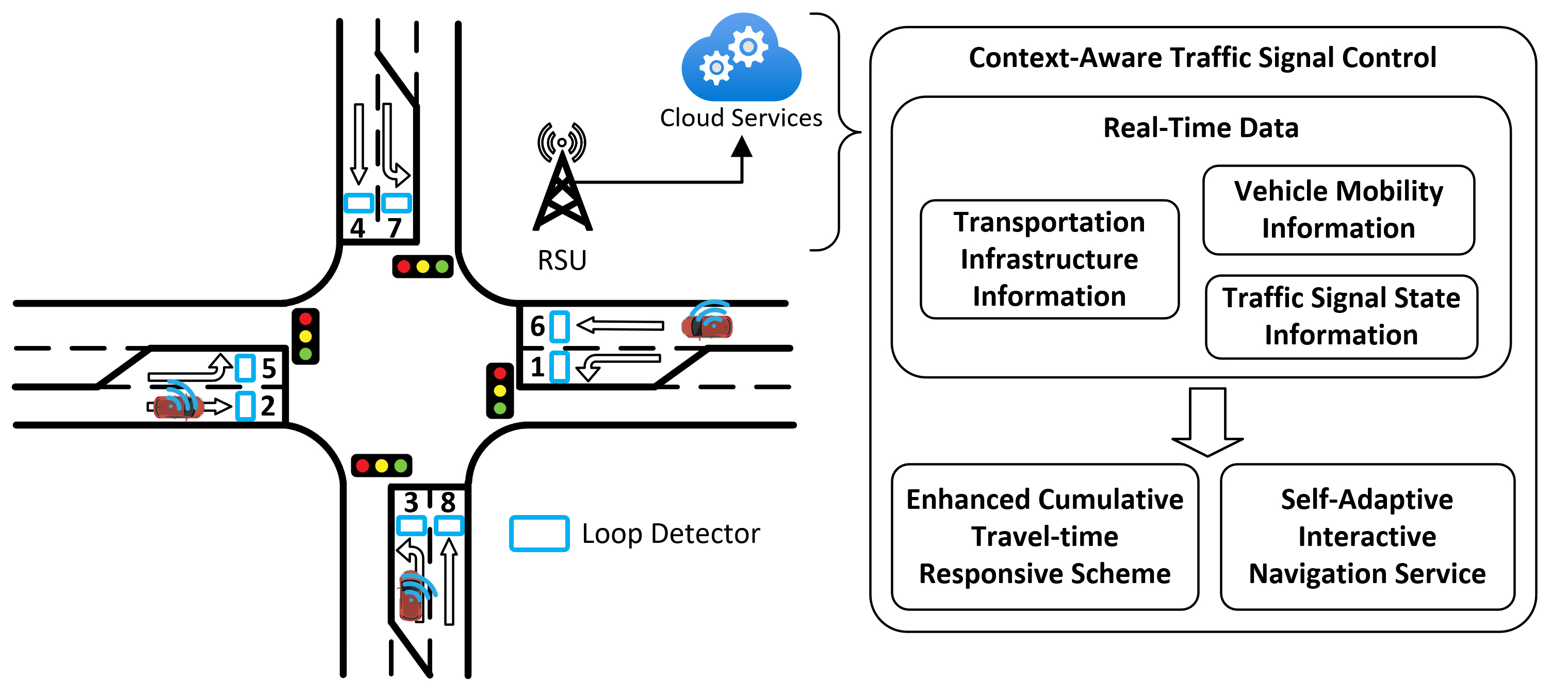
To address these gaps, we propose CATS, a Context-Aware Traffic Signal control system that tightly co-designs intersection signal control and road navigation for CAVs, as illustrated in Figure 1. With the transportation infrastructure information, vehicle mobility information, and traffic signal state information,CATS integrates two components built on top of existing foundations: Best-Combination CTR (BC-CTR) and the Self-Adaptive Interactive Navigation Tool (SAINT). BC-CTR enhances the original CTR scheme by first identifying the phase with the highest cumulative travel time (CTT) and then searching among its compatible phase combinations to select the group with the greatest combined CTT, thereby making more demand-aware phase-switching decisions. SAINT complements BC-CTR by computing a Congestion Contribution Step Function (CCSF) for each vehicle to quantify how much remaining congestion lies ahead on its route, and uses this to steer newly arriving vehicles toward less-congested paths. Because SAINT incorporates traffic-signal waiting time into its path-cost estimate, it remains consistent with the phase decisions made by BC-CTR, enabling the two components to interact and produce combined improvements in both E2E travel time and network throughput.
In this paper, the term context-aware refers to using both local intersection state and network-level route context for control decisions, rather than relying on local demand only. Specifically, CATS uses (i) phase-level and compatible-group CTT at each intersection, (ii) road-segment delay and route-level E2E delay estimated from network traffic observations, (iii) CCSF-based congestion contribution values that indicate downstream congestion remaining along each vehicle route, and (iv) expected incoming demand shaped by SAINT’s route guidance updates. Existing adaptive signal methods typically optimize phase switching from local intersection observations, while CATS additionally incorporates this network-level contextual information from navigation-side congestion estimation to better align signal timing with city-scale traffic evolution.
The key technical contributions are summarized as follows:
- We design BC-CTR, an enhanced actuated signal control scheme that extends the original CTR by first selecting the phase with the highest cumulative travel time (CTT) and then identifying the compatible phase combination with the greatest group CTT. This two-step selection allows the controller to respond more accurately to real-time intersection demand than the single-combination evaluation in the original CTR.
- We integrate BC-CTR with SAINT, a congestion-contribution-based navigation service, into a unified CATS framework. SAINT quantify remaining congestion on each vehicle’s route and steers incoming vehicles toward less-congested paths, while incorporating traffic-signal waiting time into path costs so that navigation remains consistent with BC-CTR’s signal decisions.
- We evaluate CATS through SUMO-based simulations spanning heavy to light traffic, comparing with three baselines. Under moderate-to-heavy traffic, CATS reduces mean E2E travel time by up to 23.72% and improves throughput by up to 93.19% over the baselines, demonstrating that the co-design of navigation and signal control produces complementary benefits.
The rest of this paper is organized as follows. Section 2 summarizes and analyzes the existing related work. Section 3 describes the system design of our proposed method, which includes the preliminary schemes. Section 4 shows the performance evaluation of the proposed system. Section 5 discusses the implications of our results and potential limitations. Finally, in Section 6, we conclude this paper along with future work.
2. Related Work
In this section, we introduce the related work for optimizing traffic signal control. We surveyed the recent studies on traffic signal control optimization, categorizing them into three main approaches: fixed-time-oriented optimization, adaptive signal control, and integrated navigation-signal control.
For fixed-time-oriented optimization, recent studies include probe-data-assisted timing design [5], network-level joint signal/trajectory optimization for mixed traffic [6], bee-colony-based plan search for superstreet fixed-time control [7], coordinated offset optimization via flow- and bandwidth-based formulations [8], constrained cycle/split optimization for isolated intersections under environmental and non-motorized constraints [19], vision-assisted multi-intersection timing updates [20], and method-level optimization for urban multi-leg intersections [21]. Their main benefit is improved delay, progression, or emissions under target scenarios, but common limitations remain: strong dependence on scenario-specific demand assumptions, limited robustness under incident-driven nonstationary traffic, and reduced transferability when network geometry, sensing quality, or connected-vehicle penetration changes.
Recent adaptive signal-control studies mainly adopt learning-based methods. Cao et al. [9] apply deep reinforcement learning to optimize phase-switching decisions from real-time intersection states, while Cai and Wei [10] improve DQN-style training stability for urban adaptive control under varying demand. Kamal et al. [11] combine a digital twin with deep reinforcement learning to reduce the simulation-to-deployment gap during policy development. Mo et al. [12] propose a decentralized connected-vehicle-based learning framework (CVLight) to improve scalability and local responsiveness. Fu et al. [13] present an improved D3QN phase-control strategy for isolated intersections to better balance delay and queue evolution. Although these studies report improved delay or throughput, common limitations remain: many evaluations are conducted in simulated or isolated-intersection settings, performance can depend on penetration and quality of connected-vehicle sensing, and policy transferability across cities and mixed traffic compositions is still limited.
Moreover, recent studies have explicitly integrated traffic signal control with navigation and route guidance. Cao et al. [14] use navigation requests to reserve coordinated green-wave opportunities, Menelaou et al. [15] jointly optimize route guidance and regional demand management for real-time network control, Guo et al. [16] proactively coordinate guidance and signal control in divergent networks, Zhang et al. [17] couple dynamic route guidance with signal timing under accident-induced congestion, and De Souza et al. [18] formulate a joint routing-signal multi-commodity optimization for connected vehicles. These approaches improve progression, throughput, or resilience in targeted scenarios, but common limitations include assumptions on communication reliability and penetration, high computational/coordination overhead at scale, and limited validation under heterogeneous real-world driver compliance.
However, most existing systems do not fully leverage the potential of context-aware data from navigation services to optimize traffic signal control. In this work, we aim to fill this gap by proposing a context-aware traffic signal control optimization system that integrates road navigation services for improved traffic management. Table 1 summarizes the main differences between the representative approach categories and CATS.
3. System Design
In this section, we first give a brief overview of the original CTR scheme and SAINT system, which are the basis of our proposed system. Then, we introduce the design of our proposed Context-aware Traffic Signal (CATS) control optimization system, which integrates an enhanced CTR scheme and SAINT system to improve road traveling efficiency.
3.1. Preliminaries
The original CTR scheme and SAINT system are the basis of our proposed system. CTR scheme is an actuated traffic signal control method that adjusts traffic signal timings based on the cumulative travel time (CTT) of vehicles approaching an intersection. The SAINT navigation system provides real-time route guidance to drivers based on current traffic conditions, utilizing a congestion prediction mechanism to suggest optimal routes that minimize travel time and avoid congested areas.
3.1.1. Cumulative Travel-Time Respoinsive Scheme (CTR)
The cumulative travel-time responsive (CTR) [4,22] scheme is an actuated traffic signal control method that adjusts traffic signal timings based on the cumulative travel time (CTT) of vehicles approaching an intersection. The CTT is defined as the summation of driving time of all vehicles at current phase (road or lane) of a road segment. As shown in Figure 2, assume that there are multiple phases at an intersection, each phase corresponds to a specific movement direction (e.g., straight, left turn, right turn) for vehicles approaching the intersection from different road segments. We can calculate the CTT for each phase by summing the travel times of all vehicles waiting at that phase. Specifically, assume that there are n vehicles at phase i, and the travel time of vehicle j is , then the CTT of phase i can be calculated as follows:
Figure 3 illustrates the working principle of the CTR scheme. When starting, the CTR scheme checks the CTT of each phase at an intersection. And then, it selects the phase (i.e., ) with the highest CTT to compare it with the current phase (i.e., ). If the CTT of is larger than that of by a predefined threshold, the traffic signal will switch to green for , allowing vehicles to pass through the intersection. Otherwise, the current phase will continue to have the green signal. Either case, based on a timer the CTR scheme will periodically check the CTT of each phase to make further decisions. The timer is generally set to a few seconds (e.g., 5 seconds) to ensure timely response to changing traffic conditions.
As shown in Figure 3, by monitoring the CTT, the CTR scheme can dynamically allocate green signal time to phases with higher traffic demand, thereby improving traffic flow and reducing congestion at intersections.
3.1.2. Self-Adaptive Interactive Navigation Tool (SAINT)
The self-adaptive interactive navigation tool (SAINT) [23,24] is a road navigation service that provides real-time route guidance to drivers based on current traffic conditions. It utilizes a congestion prediction mechanism to suggest optimal routes that minimize travel time and avoid congested areas.
The congestion prediction mechanism relies on the travel time of each road segment. In practice, the travel time of an individual road segment or an E2E path can be measured using various methods, such as cameras or loop detectors. Assume that, during a sampling period T, the number of vehicles traveling on road segment is n, where denotes an edge connecting vertices and . Let denote the travel time of vehicle on this segment. Then, the mean travel delay for road segment is calculated as follows,
where denotes the length of road segment , denotes its speed limit, and denotes the average traffic-light waiting time. Equation (2) considers two cases. If vehicles are traveling on the road segment during the sampling period, is calculated as the average travel time of those vehicles. If no vehicle travels on the segment during the sampling period, is estimated as the travel time based on the segment length and speed limit, plus the average traffic-light waiting time. Note that includes the waiting time at the traffic light at the intersection before the vehicle enters the next road segment.
For a vehicle whose route consists of a sequence of intersections, , where , the E2E delay can be expressed as:
where denotes the set of intersections included in the route of vehicle .
Based on the road segment delay and E2E delay, each vehicle is associated with a travel delay on each road segment along its route, referred to as the link delay, as well as an E2E delay for the entire route. For a particular vehicle , the congestion contribution (CC) is defined as:
where denotes the E2E delay of vehicle for a travel path with n vertices, that is, the travel delay from source intersection 1 to destination intersection n, and denotes the sub-route delay from source intersection 1 to an intermediate intersection i:
where denotes the travel delay of road segment in the route. Note that is defined as 0 because it represents the delay at the start of the route, and the corresponding CC value is 1.
Since remains invariant on each road segment of a route, we define the Congestion Contribution Step Function (CCSF) for the sub-route delay x from the vehicle’s starting position to an intermediate position on its trajectory:
where is a shifted unit step function defined as:
As shown in Figure 4, for the vehicle a set of the CC values is calculated based on the CCSF (6) that decreases CC values of a road segment where the vehicle will travel. The whole road network is updated by the CC values from all vehicles and each road segment has a weight value . The route of the vehicle virtually affects new joined vehicles in the whole road network. The new joined vehicles are navigated by the less congested path.
In the next section, we introduce the design of our proposed Context-aware Traffic Signal (CATS) control optimization system, which integrates an enhanced CTR scheme and SAINT system to enhance traffic signal control and navigation services.
3.2. Context-Aware Traffic Signal (CATS) Control System
In this section, we describe the design of Context-Aware Traffic Signal (CATS) control system. We first introduce the design of the enhanced CTR scheme, which is a key component of CATS. Then, we describe how to integrate the enhanced CTR scheme with SAINT to achieve better performance in terms of traffic flow throughput and travel time.
3.2.1. Enhanced CTR
CTR controls traffic signals of an intersection by monitoring cumulative travel time (CTT) from each incoming road segment. The CTT is defined as the summation of driving time of all vehicles at current phase (lane) of a road segment, as shown in Figure 2. The CTT of a phase at an intersection changes by vehicle traffic. When the CTT of a phase becomes the largest among all CTTs of phases, the traffic signal of this phase shall be switched to green signal for vehicles passing.
As shown in Figure 5, assuming that phase 6 has the largest CTT among all phases, the original CTR will directly select the phase combination of phase 6 (i.e., the option B) to switch to green signal. In contrast, our proposed enhanced CTR will select the compatible phases of phase 6, and then compare the group CTT of the compatible phases (e.g., phase 2 and phase 1) of phase 6 to make switching decision. In Figure 5, there could be two options to swtich traffic signals. Option B is to select the phase 6 and 1, where as option A is to select the phase 6 and 2 since they are compatible. The enhanced CTR will compare the group CTT of the phase combination of phase 6 and phase 2 with the group CTT of the phase combination of phase 6 and phase 1, and select the one with larger group CTT to switch to green signal. In this way, the enhanced CTR can better reflect the real-time traffic status by considering more traffic information from compatible phases, which can lead to better performance in terms of traffic flow and congestion reduction. We call the enhanced CTR as Best-Combination CTR (BC-CTR), since it considers the best combination of phases for the current traffic status.
On top of the original CTR scheme, we formalize BC-CTR as follows. For a signalized intersection, let the phase set be , and let denote the CTT of phase i at decision epoch k. We first select the primary phase as
To model movement conflicts (e.g., a protected left turn conflicting with opposite through traffic), we define a binary conflict matrix , where
Using , the set of feasible compatible phase groups containing the primary phase is
For each candidate group , BC-CTR computes the group CTT
and selects
Let denote the currently active compatible group. BC-CTR switches to only when
where is the same switching threshold concept used in CTR; otherwise, it keeps the current group. Therefore, conflicts are handled explicitly by the constraint , and only pairwise non-conflicting phase combinations are admissible for green allocation.
3.2.2. Working Process of CATS
The working process of BC-CTR is shown in Figure 6. BC-CTR has a timer to periodically check the vehicle traffic status, e.g., every 5 seconds. When the timer is end, CTT of each phase at an intersection will be calculated. Then BC-CTR finds the phase with the largest CTT and searches for its compatible phases. The compatible phases can be classified into 2 groups, current group (CG) and opposite group (OG). For each group, the group CTT is calculated by summing the CTTs of all phases in the group. BC-CTR will compare the CTTs of the two groups, and select the group with larger CTT to generate traffic signal states. The generated traffic signal states will be compared with the current traffic signal states to make switching decision. If the generated traffic signal states are different from the current traffic signal states, the traffic signals will be switched to the generated traffic signal states. Otherwise, the current traffic signal states will be maintained. This process will be repeated periodically to adapt to the changing traffic conditions at the intersection.
3.2.3. Integration with Road Navigation Services
CATS integrates the proposed BC-CTR and the SAINT system to provide a better driving experience in a traffic-signal rich area. When a vehicle requests a route guidance from SAINT, SAINT will provide an optimized route based on current traffic status and projected traffic conditions in the future. During the vehicle driving along the suggested route, BC-CTR will control traffic signals at intersections based on real-time vehicle traffic status.
Since SAINT considers the waiting time at traffic signals in its route guidance, though the traffic signals are controlled by BC-CTR, SAINT can still provide an optimized route for the vehicle. More specifically, in the integrated CATS setting we interpret the link cost used by SAINT as the sum of a road-travel component and a signal-delay component,
where denotes the running delay on segment , denotes the expected traffic-signal waiting delay before entering the next segment, and controls their relative importance in route selection. In this manuscript, we set , because both terms are measured in seconds and jointly contribute to end-to-end travel time. Therefore, the integrated path cost is additive and can be written consistently with Equation (2); when observed travel samples are available, the signal-waiting component is already included in the measured link travel time, and when no sample is available, the estimate uses free-flow segment travel time plus average signal delay. This formulation explains how SAINT balances road-segment delay and signal delay while remaining consistent with the signal states generated by BC-CTR.
In this way, the navigation and signal control components of CATS are tightly integrated. BC-CTR optimizes signal timings based on real-time traffic conditions, while SAINT provides route guidance that accounts for both road congestion and expected signal delays. This co-design allows CATS to achieve better performance in terms of traffic flow throughput and travel time compared to systems that optimize navigation and signal control separately.
4. Performance Evaluation
We use SUMO (Simulation of Urban MObility) [25] to conduct simulations. The grid road network is generated by NETGENERATE tool in SUMO. For measuring road segment travel time, we use TLSE3Detectors tool in SUMO to generate loop detectors. For the loop detectors, instead of using the default detected inforamtion (e.g., speed, vehicle count, occupancy) by a pair of loop detectors at a single location of a road segment, by two pairs of detectors located at two ends of a road segment we modified the original function to calculate the travel time of each vehicle on the road segment so that the mean travel time of the road segment for a given time interval can be calculated. We use the TraCI [25] APIs of SUMO to control all the process of CATS. The simulation environment is shown in Figure 8.

Figure 7.
Simulation Setup.
Other simulation environment parameters are in Table 2. For the road networks, we use a grid road network for simulation. In this grid road network, each road segment has 3 lanes with a dedicated lane for left turns. To make the simulation more realistic, we add 2-second yellow signal time for the transition between green and red signals. This transition time can mitigate aggressive driving behaviors of vehicles inside intersection areas due to sudden traffic light switching. The road network used in the simulation can reflect a real-world traffic-signal rich area (e.g., Manhattan area), where there are many intersections with traffic signals.
For the performance metrics, we measure both throughput and E2E travel time.
- Throughput: The total number of vehicles departing from and arriving at the fixed locations that successfully pass through the road network during the simulation period.
- End-to-End (E2E) Travel Time: The total time taken for a vehicle from the fixed locations to travel from its departure point to its destination, including any waiting time at traffic signals.
To measure throughput, the vehicle traffic is configured to be injected to move from one-side boundary to the opposite-side boundary, depicted by the blue arrows at the boundaries in Figure 8, and two pairs of fixed locations are selected for E2E travel time measurement (i.e., Location Pair 1 and 2 as shown in Figure 8). To get E2E travel time, we let 20 vehicles depart from the two pairs of the fixed locations in the grid road network. For these 20 vehicles, their actual navigated routes may be different depending on the traffic status. The conducted simulations are open-loop, that is, if a vehicle arrives at its destination, it will be removed from the simulation.
The vehicle speed limit is set to 80 km/h, which is a common speed limit in urban areas. The vehicle inter-arrival time is set to 5s, 7s, 9s, 11s, 13s, and 15s to evaluate the performance under different traffic conditions, ranging from heavy traffic (5s inter-arrival time) to light traffic (15s inter-arrival time). All the peroformance metrics are averaged over 10 simulation runs for each setting to ensure the reliability of the results. And the results include 90% confidence intervals to show the variability of the performance metrics across different runs.
To demostrate the improvement of the proposed CATS method, we compare it with several baseline methods, which are combinations of two traffic signal control methods, i.e., BC-CTR (Best-Combination-CTR) and O-CTR (Original-CTR) and two navigation methods (i.e., SAINT and Dijkstra).:
- 1.
- Dijkstra + BC-CTR
- 2.
- SAINT + O-CTR
- 3.
- Dijkstra + O-CTR
4.1. Mean E2E Travel Time
To evaluate the mean End-to-End (E2E) travel time, we varied vehicle inter-arrival time to generate different traffic states, i.e. from heavy traffic to light traffic, in the simulation. As shown in Figure 9, the mean E2E travel time of CATS (i.e., SAINT with BC-CTR) is the lowest among the 4 combinations when the vehicle inter-arrival time is large (i.e., 5s, 7s, and 9s). This observation suggests that the proposed CATS method can better reflect the real-time traffic status by considering more traffic information from compatible phases, which can lead to better performance in terms of traffic flow and congestion reduction. However, when the vehicle inter-arrival time increases (i.e., 11s, 13s, and 15s), the mean E2E travel time of CATS is almost same as that of SAINT with O-CTR as well as other baselines. This observation suggests that when the traffic is light, the performance of CATS and the baselines is similar, since the traffic status is not heavy enough to show the advantage of CATS. In contrast, when the traffic is heavy, CATS can better optimize the traffic signal control by considering more traffic information, leading to lower E2E travel time.
Figure 10 shows the cumulative distribution function (CDF) of mean E2E travel time for CATS and other baselines. From the figure, we can see that the CDF of mean E2E travel time of CATS is higher than that of the other combinations mostly. This observation further confirms that CATS can better optimize the traffic signal control under heavy traffic conditions, leading to lower E2E travel time for vehicles. However, when the vehicle inter-arrival time increases (i.e., 11s, 13s, and 15s), the CDF of mean E2E travel time of CATS is almost same as that of other baselines.
More specifically, CATS achieves mean E2E travel times of 1154.3, 949.0, 423.6, 327.9, 304.3, and 290.2 s at inter-arrival times of 5, 7, 9, 11, 13, and 15 s, respectively. Compared with SAINT+O-CTR, CATS reduces the mean E2E travel time by 275.6 s (19.27%) at 5 s, 152.5 s (26.47%) at 9 s, 44.3 s (11.91%) at 11 s, 32.7 s (9.71%) at 13 s, and 29.4 s (9.19%) at 15 s. Averaged over the heavier traffic cases of 5, 7, and 9 s, CATS reduces the mean E2E travel time by 13.40% compared with SAINT+O-CTR, 23.72% compared with Dijkstra+BC-CTR, and 16.08% compared with Dijkstra+O-CTR. The largest single reduction is observed at 9 s, where CATS lowers the mean E2E travel time by 296.8 s (41.20%) relative to Dijkstra+BC-CTR and by 389.5 s (47.90%) relative to Dijkstra+O-CTR. These results indicate that the integration of SAINT with BC-CTR is particularly effective in the moderate-to-heavy traffic region.
The CDF figure shows a more nuanced pattern. At the median point, CATS reaches about 324.2 s, which is 42.6 s (11.61%) lower than SAINT+O-CTR and 155.4 s (32.40%) lower than Dijkstra+O-CTR, but only 8.4 s (2.51%) lower than Dijkstra+BC-CTR. At the 90th percentile, CATS reaches about 1100.8 s, which is still 181.9 s (14.18%) lower than SAINT+O-CTR and 36.6 s (3.22%) lower than Dijkstra+O-CTR. However, unlike the throughput figure (Figure 11), the CATS CDF does not strictly dominate all other schemes over the entire range. One unusual observation is that SAINT+O-CTR is slightly better than CATS at 7 s in the mean plot, reducing travel time by 37.0 s (4.05%) relative to CATS. Another notable point is that the CDF curves cross each other: Dijkstra+BC-CTR has a slightly smaller 25th-percentile value than CATS (284.8 s versus 288.8 s), and CATS has a larger 75th-percentile value than all three baselines (907.0 s versus 833.0 s for SAINT+O-CTR, 761.0 s for Dijkstra+BC-CTR, and 901.7 s for Dijkstra+O-CTR). This suggests that although CATS yields the best average E2E travel time overall, it still exhibits a heavier upper-tail delay in part of the distribution.
4.2. The Mean Throughput
Figure 11 shows the mean throughput of CATS and other baselines under different vehicle inter-arrival times. From the figure, we can see that the mean throughput of CATS is higher than that of the other combinations when the vehicle inter-arrival time is small (i.e., 5s, 7s, and 9s). This observation suggests that CATS can better optimize the traffic signal control under heavy traffic conditions, leading to higher throughput for vehicles. However, when the vehicle inter-arrival time increases (i.e., 11s, 13s, and 15s), the mean throughput of CATS is almost same as that of other baselines. This observation suggests that when the traffic is light, the performance of CATS and the baselines is similar, since the traffic status is not heavy enough to show the advantage of CATS.
Figure 12 shows the CDF of mean throughput for CATS and other baselines. From the figure, we can see that the CDF of mean throughput of CATS is higher than that of the other combinations mostly. This observation further confirms that CATS can better optimize the traffic signal control under heavy traffic conditions, leading to higher throughput for vehicles. However, when the vehicle inter-arrival time increases (i.e., 11s, 13s, and 15s), the CDF of mean throughput of CATS is almost same as that of other baselines.
More specifically, CATS achieves throughput values of 4015.9, 7207.1, 12524.3, 10539.8, 9040.7, and 7927.1 vehicles at inter-arrival times of 5, 7, 9, 11, 13, and 15 s, respectively. Compared with SAINT+O-CTR, the throughput gains of CATS are 13.5 (0.34%), 727.2 (11.22%), 464.3 (3.85%), 83.0 (0.79%), 64.7 (0.72%), and 56.4 (0.72%) vehicles, respectively. Averaged over the heavier traffic cases of 5, 7, and 9 s, CATS improves throughput by 5.35% over SAINT+O-CTR, 93.19% over Dijkstra+BC-CTR, and 81.15% over Dijkstra+O-CTR. The largest single gain is observed at 9 s, where CATS outperforms Dijkstra+BC-CTR by 6950.0 vehicles (124.68%) and Dijkstra+O-CTR by 6311.5 vehicles (101.59%). These results indicate that the navigation component is the dominant factor in throughput improvement, while BC-CTR provides an additional gain on top of SAINT.
The CDF figure shows the same trend from a distribution perspective. At the 25th, 50th, 75th, and 90th percentiles, CATS reaches throughput values of about 6100, 7923, 10533, and 12520, respectively. Relative to SAINT+O-CTR, these percentile gains are 38 (0.63%), 52 (0.66%), 90 (0.86%), and 493 (4.10%) vehicles, while the gains over Dijkstra+BC-CTR are much larger, namely 42.62%, 30.48%, 17.77%, and 23.13%. One unusual observation is that Dijkstra+BC-CTR is slightly worse than Dijkstra+O-CTR under the heavier traffic cases of 5, 7, and 9 s, indicating that BC-CTR alone does not guarantee a throughput gain without the SAINT navigation support. Another notable point is that throughput is not monotonic with increasing inter-arrival time: all schemes peak around 9–11 s and then decrease at 13 and 15 s because lighter traffic injects fewer vehicles into the road network. In addition, the gain of CATS over SAINT+O-CTR is very small at the most congested 5 s case, but becomes much clearer at 7 and 9 s, suggesting that the benefit of the proposed integration is most visible under moderate-to-heavy traffic rather than at the most saturated operating point.
Overall, the performance evaluation shows that CATS delivers the clearest benefit under moderate-to-heavy traffic. Averaged over the 5, 7, and 9 s inter-arrival settings, CATS reduces mean E2E travel time by 13.40% relative to SAINT+O-CTR, 23.72% relative to Dijkstra+BC-CTR, and 16.08% relative to Dijkstra+O-CTR, while improving throughput by 5.35%, 93.19%, and 81.15% over the same baselines, respectively. The strongest single-case gains appear at 9 s, where CATS lowers mean E2E travel time by up to 389.5 s (47.90%) and increases throughput by up to 6950.0 vehicles (124.68%), indicating that the integration of SAINT and BC-CTR produces substantial complementary benefits when congestion is significant.
5. Limitations
One limitation of the current CTR design is that it uses phase-based CTT calculation, meaning that CTT is computed for each lane. In practice, however, some vehicles may travel in a lane that does not match their intended turning direction. As a result, their travel times are counted toward the CTT of the lane they currently occupy rather than the movement they actually intend to take, which can reduce the accuracy of the CTT representation.
Another limitation is that the current evaluation is conducted only in a simulated grid road network with a fixed road-segment length, speed limit, signal-transition setting, and vehicle inter-arrival patterns. Although this setup is useful for controlled comparison, it does not fully capture the diversity of irregular urban networks, heterogeneous intersection layouts, lane drops, incidents, pedestrian phases, bus stops, or communication failures that may affect practical deployment. Relatedly, the simulation assumes that navigation guidance and traffic data are available in a timely and reliable manner, whereas real deployments may experience sensing noise, delayed updates, packet loss, and imperfect compliance by human drivers.
The reported results are also limited by the scope of the performance metrics and baselines. We mainly evaluate throughput and E2E travel time, but do not explicitly analyze other important criteria such as queue length, fairness among movements, fuel consumption, emissions, safety-related surrogate metrics, or computational overhead at large scale. In addition, the comparison is restricted to combinations of SAINT, Dijkstra, BC-CTR, and O-CTR. Therefore, the current results show the relative benefit of CATS within this comparison set, but they do not yet establish how CATS would perform against a broader set of modern adaptive or learning-based traffic signal control methods.
Finally, the E2E-delay results indicate that the proposed method does not uniformly dominate the alternatives across the entire distribution. In particular, some CDF curves cross each other and SAINT+O-CTR performs slightly better than CATS in one mean-delay setting. This implies that, while CATS improves average performance overall, it can still produce unfavorable upper-tail delay behavior in some traffic regimes. A more complete validation therefore requires larger-scale experiments over additional network topologies, longer time horizons, richer demand patterns, and real-world or hardware-in-the-loop data.
6. Conclusions
In this paper, we proposed CATS, a context-aware traffic signal control system that combines BC-CTR with SAINT to jointly optimize phase switching and route guidance for CAVs. BC-CTR improves the original CTR by selecting the highest-CTT phase first and then choosing the compatible phase combination with the largest group CTT, while SAINT steers vehicles away from congested paths using congestion-aware route guidance. SUMO-based simulations show that under moderate-to-heavy traffic (5–9 s inter-arrival time), CATS reduces mean E2E travel time by 13.40%, 23.72%, and 16.08% over SAINT+O-CTR, Dijkstra+BC-CTR, and Dijkstra+O-CTR, respectively, and improves throughput by 5.35%, 93.19%, and 81.15% over the same baselines. Future work will focus on movement-aware CTT calculation and integrating a learning-based phase-switching mechanism into BC-CTR to better handle heterogeneous traffic demand and irregular real-world road networks.
Author Contributions
Conceptualization, methodology, software, validation, formal analysis, investigation, resources, data curation, writing—original draft preparation, writing—review and editing, visualization, supervision, project administration, funding acquisition, Y. Shen.
Funding
This research was funded by in part by Basic Science Research Program through the National Research Foundation of Korea (NRF) funded by the Ministry of Education (NRF-2022R1I1A1A01053915), in part by the MSIT (Ministry of Science and ICT), Korea, under the National Program for Excellence in SW (2022-0-01077) supervised by the IITP (Institute of Information & communications Technology Planning & Evaluation) in 2025, and in part by Ajou University research fund.
Acknowledgments
During the preparation of this study, the author(s) used GitHub Copilot for the purposes of polishing up texts. The authors have reviewed and edited the output and take full responsibility for the content of this publication. The author(s) would like to thank Prof. Jaehoon (Paul) Jeong, Dr. Jinho Lee, Dr. Saerona Choi, and Prof. Byungkyu (Brian) Park for their valuable comments and suggestions to improve the quality of this paper.
Conflicts of Interest
The authors declare no conflicts of interest. The funders had no role in the design of the study; in the collection, analysis, or interpretation of data; in the writing of the manuscript; or in the decision to publish the results.
References
- Jeong, H.; Shen, Y.; Jeong, J.; Oh, T. A comprehensive survey on vehicular networking for safe and efficient driving in smart transportation: A focus on systems, protocols, and applications. Vehicular Communications 2021, 31, 100349. [Google Scholar] [CrossRef]
- Rottenstreich, O.; Buchnik, E.; Ferster, S.; Kalvari, T.; Karliner, D.; Litov, O.; Tur, N.; Veikherman, D.; Zagoury, A.; Haddad, J.; et al. Probe-based study of traffic variability for the design of traffic light plans. In Proceedings of the 2024 16th International Conference on COMmunication Systems & NETworkS (COMSNETS). IEEE, 2024; pp. 353–360. [Google Scholar] [CrossRef]
- Mahmud, S.; Day, C.M. Infrastructure-Free Optimization of Traffic Signal Offsets: Identifying Traffic Flow Patterns and Reverse Engineering Signal Timing with Connected Vehicle Data. Transportation Research Record 2025, 03611981251378136. [Google Scholar] [CrossRef]
- Lee, J.; Park, B.B.; Yun, I. Cumulative Travel-Time Responsive Real-Time Intersection Control Algorithm in the Connected Vehicle Environment. Journal of Transportation Engineering 2013, 139, 1020–1029. [Google Scholar] [CrossRef]
- Li, Y.; Peng, L. Elevating adaptive traffic signal control in semi-autonomous traffic dynamics by using connected and automated vehicles as probes. IET Intelligent Transport Systems 2024, 18, 1016–1030. [Google Scholar] [CrossRef]
- Niroumand, R.; Kafashan, F.; Hajibabai, L.; Hajbabaie, A. Real-time network-level traffic signal and trajectory optimization with connected automated and human-driven vehicles. Computer-Aided Civil and Infrastructure Engineering 2025, 40, 5891–5907. [Google Scholar] [CrossRef]
- Jovanović, A.; Teodorović, D. Fixed-Time Traffic Control at Superstreet Intersections by Bee Colony Optimization. Transportation Research Record: Journal of the Transportation Research Board 2021, 2676, 228–241. [Google Scholar] [CrossRef]
- Shams, A.; Mahmud, S.; Day, C.M. Comparison of Flow- and Bandwidth-Based Methods of Traffic Signal Offset Optimization. Journal of Transportation Engineering, Part A: Systems 2023, 149. [Google Scholar] [CrossRef]
- Cao, K.; Wang, L.; Zhang, S.; Duan, L.; Jiang, G.; Sfarra, S.; Zhang, H.; Jung, H. Optimization Control of Adaptive Traffic Signal with Deep Reinforcement Learning. Electronics 2024, 13, 198. [Google Scholar] [CrossRef]
- Cai, C.; Wei, M. Adaptive urban traffic signal control based on enhanced deep reinforcement learning. Scientific Reports 2024, 14, 14116. [Google Scholar] [CrossRef] [PubMed]
- Kamal, H.; Yánez, W.; Hassan, S.; Sobhy, D. Digital-Twin-Based Deep Reinforcement Learning Approach for Adaptive Traffic Signal Control. IEEE Internet of Things Journal 2024, 11, 21946–21953. [Google Scholar] [CrossRef]
- Mo, Z.; Li, W.; Fu, Y.; Ruan, K.; Di, X. CVLight: Decentralized learning for adaptive traffic signal control with connected vehicles. Transportation Research Part C: Emerging Technologies 2022, 141, 103728. [Google Scholar] [CrossRef]
- Fu, Z.; Zhang, J.; Tao, F.; Ji, B. Traffic signal phase control at urban isolated intersections: an adaptive strategy utilizing the improved D3QN algorithm. Measurement Science and Technology 2024, 36, 016203. [Google Scholar] [CrossRef]
- Cao, M.; Li, V.O.K.; Shuai, Q. Book Your Green Wave: Exploiting Navigation Information for Intelligent Traffic Signal Control. IEEE Transactions on Vehicular Technology 2022, 71, 8225–8236. [Google Scholar] [CrossRef]
- Menelaou, C.; Timotheou, S.; Kolios, P.; Panayiotou, C.G. Joint Route Guidance and Demand Management for Real-Time Control of Multi-Regional Traffic Networks. IEEE Transactions on Intelligent Transportation Systems 2022, 23, 8302–8315. [Google Scholar] [CrossRef]
- Guo, Y.; Zhang, K.; Chen, X.; Li, M. Proactive Coordination of Traffic Guidance and Signal Control for a Divergent Network. Mathematics 2023, 11, 4262. [Google Scholar] [CrossRef]
- Zhang, H.; Guo, S.; Long, X.; Hao, Y. Combined Dynamic Route Guidance and Signal Timing Optimization for Urban Traffic Congestion Caused by Accidents. Journal of Advanced Transportation 2023, 2023, 1–16. [Google Scholar] [CrossRef]
- De Souza, F.; Carlson, R.C.; Muller, E.R.; Ampountolas, K. Multi-Commodity Traffic Signal Control and Routing With Connected Vehicles. IEEE Transactions on Intelligent Transportation Systems 2022, 23, 4111–4121. [Google Scholar] [CrossRef]
- Tran, Q.H.; Do, V.M.; Dinh, T.H. Traffic signal timing optimization for isolated urban intersections considering environmental problems and non-motorized vehicles by using constrained optimization solutions. Innovative Infrastructure Solutions 2022, 7. [Google Scholar] [CrossRef]
- Zhou, S.; Ng, S.T.; Yang, Y.; Xu, J.F. Integrating computer vision and traffic modeling for near-real-time signal timing optimization of multiple intersections. Sustainable Cities and Society 2021, 68, 102775. [Google Scholar] [CrossRef]
- Ma, Q.; Zeng, H.; Wang, Q.; ullah, S. Traffic Optimization Methods of Urban Multi-leg Intersections. International Journal of Intelligent Transportation Systems Research 2021, 19, 417–428. [Google Scholar] [CrossRef]
- Choi, S.; Park, B.B.; Lee, J.; Lee, H.; Son, S.H. Field implementation feasibility study of cumulative travel-time responsive (CTR) traffic signal control algorithm. Journal of Advanced Transportation 2016, 50, 2226–2238. [Google Scholar] [CrossRef]
- Jeong, J.; Jeong, H.; Lee, E.; Oh, T.; Du, D.H.C. SAINT: Self-Adaptive Interactive Navigation Tool for Cloud-Based Vehicular Traffic Optimization. IEEE Transactions on Vehicular Technology 2016, 65, 4053–4067. [Google Scholar] [CrossRef]
- Shen, Y.; Lee, J.; Jeong, H.; Jeong, J.; Lee, E.; Du, D.H.C. SAINT+: Self-Adaptive Interactive Navigation Tool+ for Emergency Service Delivery Optimization. IEEE Transactions on Intelligent Transportation Systems 2018, 19, 1038–1053. [Google Scholar] [CrossRef]
- Lopez, P.A.; Behrisch, M.; Bieker-Walz, L.; Erdmann, J.; Flötteröd, Y.P.; Hilbrich, R.; Lücken, L.; Rummel, J.; Wagner, P.; Wiessner, E. Microscopic Traffic Simulation using SUMO. In Proceedings of the 2018 21st International Conference on Intelligent Transportation Systems (ITSC), 2018; pp. 2575–2582. [Google Scholar] [CrossRef]
Figure 1.
Overview of CATS Architecture.

Figure 2.
Calculation of Cumulative Travel-time Value.

Figure 3.
Cumulative Travel-time Responsive (CTR) Scheme.

Figure 4.
Congestion Contribution Concept in SAINT.

Figure 5.
An Example of the Phase Selection Scenario.

Figure 6.
BC-CTR Working Process.

Figure 8.
Road Networks in the Simulation Environment.

Figure 9.
Mean E2E Travel Time.

Figure 10.
The CDF of Mean E2E Travel Time.

Figure 11.
Mean Throughput.

Figure 12.
The CDF of Mean Throughput.


Table 1.
Comparison of Existing Approaches and the Proposed CATS.
| Approach | Real-Time | Network-Wide | Route–Signal | Lightweight | E2E + Throughput |
|---|---|---|---|---|---|
| Adaptation | Context | Integration | Online Logic | Evaluation | |
| Fixed-time-oriented | × | × | × | ✓ | × |
| Adaptive signal control | ✓ | × | × | × | × |
| Integrated navigation-signal | ✓ | ✓ | ✓ | × | × |
| Proposed CATS | ✓ | ✓ | ✓ | ✓ | ✓ |
Table 2.
Simulation Setup Configuration.
| Parameter | Configuration/Value |
|---|---|
| Road Network | A grid road network with 3 lanes per road segment |
| Road segment length | 300 meters |
| Vehicle speed limit | 80 km/h |
| Traffic Signal Control | BC-CTR, Static Traffic Light |
| Vehicle Navigation Schemes | SAINT, Dijkstra |
| Vehicle Inter-Arrival Time | 5s, 7s, 9s, 11s, 13s, 15s |
| Performance Metrics | Throughput, End-to-End (E2E) Travel Time |
| Simulation Time | 2 hours |
| Number of Runs per Setting | 10 |
Disclaimer/Publisher’s Note: The statements, opinions and data contained in all publications are solely those of the individual author(s) and contributor(s) and not of MDPI and/or the editor(s). MDPI and/or the editor(s) disclaim responsibility for any injury to people or property resulting from any ideas, methods, instructions or products referred to in the content. |
© 2026 by the authors. Licensee MDPI, Basel, Switzerland. This article is an open access article distributed under the terms and conditions of the Creative Commons Attribution (CC BY) license (http://creativecommons.org/licenses/by/4.0/).
Copyright: This open access article is published under a Creative Commons CC BY 4.0 license, which permit the free download, distribution, and reuse, provided that the author and preprint are cited in any reuse.


