Submitted:
06 March 2026
Posted:
06 March 2026
You are already at the latest version
Abstract
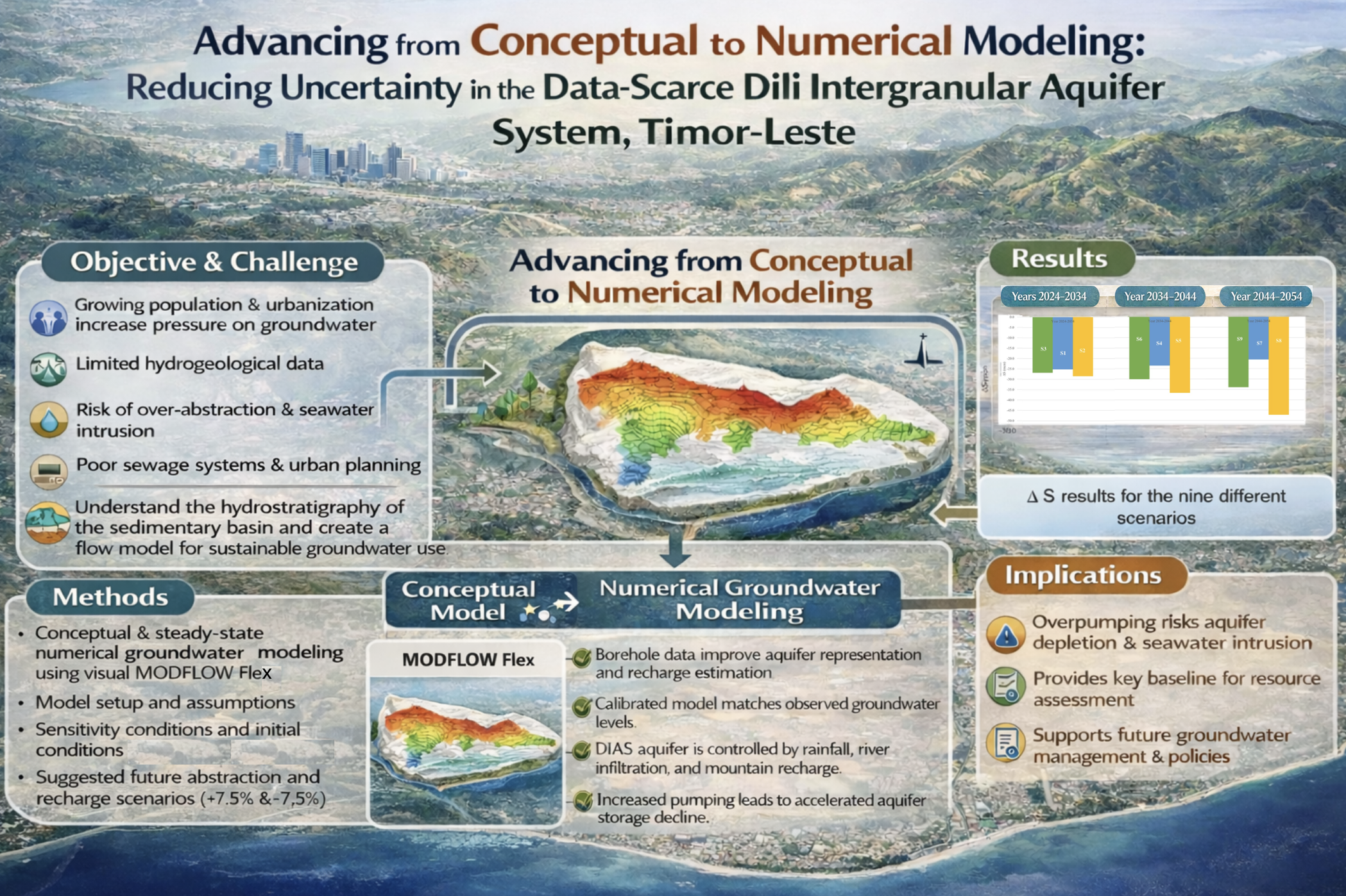
Dili, the capital of Timor-Leste, is experiencing increasing freshwater demand driven by population and economic growth. It totally relies on groundwater from the Dili Intergranular Aquifer System for supply. There is very little conceptual understanding of the system and little-to-no monitoring data. Understanding the hydrostratigraphy, recharge and surface-groundwater interactions, groundwater levels and abstractions are essential for sustainable groundwater use and management. These are the aims of this study, and a numerical model was created with such purpose. The model included scenarios to assess how the aquifer could react to future increases in groundwater abstraction. Trial and error calibrated the steady-state model, and a comparison of simulated results with observed heads revealed good agreement (RMS <10%). Transient scenario simulations demonstrate that recharge (direct, river infiltration, and mountain-block processes) is a key component of the water balance and plays a critical role in aquifer sustainability under increasing groundwater abstraction. Aquifer storage is projected to decrease significantly by 2054, with the magnitude depending on the range of recharge and abstraction rates considered. The model improves conceptual hydrogeological knowledge of the basin, highlights future work needed, and provides a robust basis for sustainable groundwater management and water risk mitigation in Dili.
Keywords:
quaternary aquifer
; conceptual modelling
; groundwater flow model
; Dili City
; Timor-Leste
Copyright: This open access article is published under a Creative Commons CC BY 4.0 license, which permit the free download, distribution, and reuse, provided that the author and preprint are cited in any reuse.


