Submitted:
04 March 2026
Posted:
09 March 2026
You are already at the latest version
Abstract
Climate extremes are critical constraints on agricultural productivity, particularly in tropical regions experiencing rapid agricultural expansion. This study examines spati-otemporal changes in soybean yields in response to droughts and heatwaves across highly productive municipalities in Brazil from 1989 to 2020. By integrating high-resolution meteorological data, satellite-derived evapotranspiration estimates, and municipal-level crop yield data, we apply standardized drought indices (Standardized Precipitation Index, Standardized Precipitation Evapotranspiration Index, and Warm Spell Duration Index) to identify climate-yield relationships across Brazil’s heterogeneous agroclimatic zones. Results reveal a marked increase in the frequency and intensity of compound drought–heat events, particularly in the Matopiba frontier, where yield sen-sitivity to hydroclimatic stress is highest. Spatial models confirm that short-term dry events, rather than long-term mean climate shifts, are the dominant drivers of recent yield variability, with significant spatial spillover effects observed across municipalities. The findings underscore the growing vulnerability of rainfed agriculture in Brazil and highlight the critical role of seasonal timing, crop phenology, and regional climate re-gimes in mediating climate risk. This study provides empirical evidence linking com-pound extremes to agricultural performance and offers a scalable framework for early warning systems and climate-resilient policy design.
Keywords:
compound events
; climate risk assessment
; agricultural resilience
1. Introduction
One of the most significant challenges of the 21st century is ensuring food security for a global population projected to exceed 10 billion people by 2050 [1]. As one of the most important crops worldwide, soybean (Glycine max) plays a critical role in addressing this challenge by serving as a major source of protein and oil [2,3]. However, soybean production is increasingly threatened by climate variability and the rising frequency, intensity, and duration of extreme hydrometeorological and climate events (EHCEs) [4]. Among these, drought and heatwave events (DHE) are significant constraints, particularly for tropical rainfed agricultural systems that are highly sensitive to climatic anomalies [5,6].
This challenge is especially relevant to Brazil, which has emerged as the world’s largest soybean producer, harvesting 169 million tonnes (~55% of global exports) in the 2024/25 season [7,8]. Although cultivated across a wide latitudinal range, from subtropical southern states to equatorial regions, Brazilian soybean yields remain highly vulnerable to climate extremes, particularly droughts [9,10,11]. Such conditions cause substantial interannual yield variability [7]. According to [12], in Southern Brazil, recurrent climatic anomalies have resulted in exceptional losses in grain production. Consecutive cropping seasons with diminished yields, particularly in 2020, 2022, and 2023, led to unharvested grains valued at approximately 8.2 billion USD (about 45 billion BRL).
The intensity and duration of droughts are rising amid increasing climate variability, underscoring the need for refined tools to monitor spatiotemporal patterns [13,14]. Process-based crop models have been widely used to simulate yield responses [15,16,17]. Nevertheless, their reliance on site-specific inputs (soil properties, cultivar traits, and management practices) often introduces calibration biases. More critically, their simplified treatment of extreme events tends to underestimate both the magnitude of climate risks and their spatial heterogeneity [18,19].
Among the available approaches to estimating drought, the Standardized Precipitation Index (SPI) quantifies precipitation over a given time scale as a standardized deviation from the long-term mean, and the Standardized Precipitation Evapotranspiration Index (SPEI) incorporates potential evapotranspiration alongside precipitation to assess available water resources. These indices provide valuable tools for characterizing drought [20,21]. They have been widely applied worldwide to assess drought trends, variability and impacts, including applications across Brazil [22,23,24].
In addition to water deficit indicators, the Warm Spell Duration Index (WSDI) offers a complementary perspective by capturing the frequency and duration of heat events, making it a valuable tool for detecting trends in heat waves and their intensification over time [25]. The WSDI is designed to measure prolonged periods of unusually warm days relative to a baseline climatology. It quantifies the number of days in a year that are part of warm spells lasting at least six consecutive days, with daily maximum temperatures exceeding the 95th percentile of a reference period. Although brief, these events can overlap with droughts and occur during critical stages of plant growth, causing damage to yield and other crop phenotypes. Together, SPI, SPEI, and WSDI provide bias-free insights into the frequency, severity, and spatial extent of drought and heatwave events across multiple timescales.
This study addresses the question: How do droughts and heatwaves affect soybean yields across Brazil’s soybean production regions? The objectives are: a) Integrate temporally variable and spatially distributed climate and soybean yield data at the municipal scale across Brazil’s soybean-producing areas; b) Identify DHE in Brazil’s soybean landscapes using relevant climate indices; c) Quantify the spatiotemporal contributions of DHE to soybean yield losses, analyzing potential drivers and underlying causes in each municipality. The study focuses on Brazil’s key soybean-producing regions, combining high-resolution climate data with SPI, SPEI, and WSDI analyses to characterize regional patterns of drought and heatwaves.
2. Materials and Methods
2.1. Study Area
A wide range of climatic conditions is observed across Brazil’s extensive territory (Figure 1a). It spans from the subtropical southern states within the Pampa and Atlantic biomes, characterized by Cfa and Cfb Köppen-Geiger climate classes, to the low-latitude regions of the Cerrado biome, the country's main agricultural frontier. In these northern regions, soybean “tropicalization” has enabled its expansion into areas with Am and Aw climate classes [26].
In this study, nine soybean-producing municipalities were selected for analyses of drought and heat indices (Figure 1; Table 1). Each municipality represents a homogeneous climatic zone (CZ) as defined by [27] and [28]. This workflow is based on the climate and agricultural representativeness of characteristic soybean production regions at the municipal level across Brazil. Additionally, the workflow and associated analytics can be expanded to include new crops and their corresponding municipalities.
To ensure consistency with the period when the crop is biologically active and water use is agronomically relevant, we used only observations occurring between the local planting start and harvest end dates, as in [29]. The soybean growing season for each municipality was defined using on the official crop calendar published by [30], which provides region specific information on planting, vegetative development, and harvest periods. For each location, the planting window, the onset of vegetative growth, and harvest dates were converted into daily time series, allowing all climate and yield observations to be filtered to the months encompassed by the respective growing season.
2.2. Soybean Yield Dataset
We analyzed annual soybean yield (Yr) data for the selected Brazilian municipalities (Table 1) from the 1996/97 to the 2019/20 crop seasons. For each municipality, the dataset included harvested area (ha) and observed yield (Yr, t ha⁻¹), obtained from the Brazilian Institute of Geography and Statistics [31]. Drought years, used for subsequent analysis of yield reductions, were defined as those with SPEI-12 < –0.5, consistent with previous studies assessing soybean yield losses in Brazil [11,21].
This section focuses on the which captures both interannual variability and long-term trends driven by technological improvements, management practices, and cultivar adoption. To isolate interannual deviations attributable to climate, was detrended using a five-year moving window, which effectively removes short- to medium-term trends while retaining year-to-year variation [11,32]. For periods at the start or end of the series, the window was adjusted to use all available data, with at least one year of observations.
For municipality and year , the detrended yield was computed as the centered moving average (Equation 1):
where represents the observed yield for years within the 5-year window.
The yield anomaly (ΔYi,t) quantifies the relative deviation of from the (Equation 2):
Positive anomalies indicate yields above the expected trend, while negative anomalies indicate yield reductions relative to the local trend.
For each crop season, we calculated the negative yield anomalies or losses () individually, estimating that for the soybean area at the municipal level. It was calculated based on the and the calculated by five-year moving windows, according to Equation 3:
where is the soybean harvested area for each municipality in year . This calculation ensures that only negative (less than zero) deviations contribute to losses, consistent with previous Brazilian soybean studies [11].
2.3. Weathear Dataset
Daily precipitation (P), maximum temperature (Tmax), minimum temperature (Tmin), relative humidity (RH), solar radiation (Rs), wind speed at 2 m height (u2), and reference evapotranspiration (ETo) were obtained from the Brazilian Daily Weather Gridded Data (BR-DWGD) dataset [33]. The dataset provides daily temporal resolution, a spatial resolution of 0.1° x 0.1°, and covers the period from 1989 to 2022 for the entire Brazilian territory. Z-score normalization was applied to standardize the scales of all climatic variables, facilitate multivariate analysis, and identify statistical outliers. This normalization reduced within-cluster variation which was essential for subsequent analytical procedures [34]. The normalized dataset was used to compute the climate indices and DHE metrics. Additionally, standardized climate indices, such as SPI, SPEI, and WSDI, were derived from the normalized BR-DWGD datasets.
2.4. Crop Evapotranspiration (ETc)
Crop coefficient (Kc) values were determined using the methodology proposed by [35] in FAO Irrigation and Drainage Paper 56. The FAO 56 procedure defines Kc as a function of the crop’s phenological stages, subdivided into initial, mid, and late-season phases. For each municipality, phase boundaries were aligned with the region-specific crop calendar, and fixed Kc values were assigned to each phase based on the mean coefficients recommended for soybean in FAO 56 and validated in recent Brazilian studies using lysimetry and remote sensing data [29,36,37].
Daily Crop Evapotranspiration (ETc) was calculated using the standard FAO 56 formulation [35] (Equation 4):
where ETo is the reference evapotranspiration, estimated using BR-DWGD for each municipality, and Kc is the stage-dependent crop coefficient assigned to each day based on the local phenological calendar [33]. This approach aligns with experimental and modeling studies that quantify soybean water use across Brazil using daily Kc curves and FAO 56 methodology [9,38].
2.5. Drought Indices
Meteorological drought was also characterized using the Standardized Precipitation Index (SPI), which is based solely on precipitation and quantifies precipitation anomalies across multiple accumulation time scales [20]. Monthly precipitation totals were aggregated over 1-, 3-, 6-, and 12-month periods to represent short- to long-term water deficits relevant to hydrometeorological and agricultural processes. For each municipality, SPI was computed independently to preserve local precipitation climatology. Accumulated precipitation series were fitted to a two-parameter Gamma distribution using maximum-likelihood estimation, following the original definition proposed by [20]. The Gamma distribution is appropriate for modeling nonnegative, right-skewed precipitation data and has been extensively validated for SPI applications across diverse climatic regimes [39]. Zero precipitation values were handled in accordance with standard SPI conventions using a mixed-probability adjustment. Cumulative probabilities derived from the fitted Gamma distribution were transformed into standardized normal variates, yielding SPI values with a mean of zero and unit variance. Negative SPI values indicate drier-than-normal conditions, while positive values indicate wetter- than-normal conditions, with larger magnitudes corresponding to greater anomaly intensity. SPI calculations were implemented in Python using a reference implementation consistent with the original methodology.
In addition to SPI, we used the Standardized Precipitation Evapotranspiration Index (SPEI), which extends the SPI framework by incorporating atmospheric evaporative demand through the climatic water balance [40]. The monthly climatic water balance was calculated as the difference between precipitation and potential evapotranspiration, and then accumulated across multiple temporal scales. SPEI was also calculated at two temporal scales, 3 and 6 months, to capture both short-term agricultural impacts and longer-term hydrological variability. The 6-month scale reflects water deficits during critical crop growth stages and is widely used to assess the effects of droughts on agricultural productivity, as documented in previous studies [40,41].
For each municipality and accumulation scale, the accumulated climatic water balance was fitted separately for each calendar month using a three-parameter Pearson Type III distribution. Monthly fitting ensures stationarity of the distributional parameters and enables consistent standardization across seasons, as recommended for drought index calculation [21,42]. The Pearson Type III distribution was selected to accommodate both negative and positive values of the water balance, preserving the physical interpretation of dry and wet periods. Cumulative probabilities from the fitted Pearson Type III distribution were transformed into standardized normal variates, yielding SPEI series with zero mean and unit variance. Negative SPEI values indicate drier-than-normal conditions, reflecting combined precipitation deficits and enhanced evaporative demand, whereas positive values indicate wetter-than-normal conditions. All SPEI calculations were performed using a custom Python implementation based on the standard SPEI methodology, adapted to use the Pearson Type III distribution for robust handling of the full range of water balance values [21,43]. Drought conditions were classified using SPEI values and standardized categories (Table 2), ranging from extreme drought (SPEI < -2.0) to non-drought or wet conditions (SPEI > 1.00).
Droughts were characterized using four key metrics derived from the SPEI time series, namely severity (cumulative SPEI during the event), duration (number of days the event persists), intensity (severity divided by duration), and peak (lowest SPEI value). These metrics provide a multidimensional understanding of drought behavior, encompassing magnitude, persistence, and extremity, which are essential for agricultural and climatological assessments [21,44].
2.6. Heatwave Index
The first step in calculating the WSDI was to determine the 95th percentile of daily maximum temperatures (Tmax) for a reference period, often using a 30-year baseline. For each day of the year, the 95th percentile (T95) was calculated from the historical temperature record (Equation 5) [45].
where T95(d) is the 95th percentile of the daily maximum temperature for day d, and Tmax (d, reference period) represents the historical maximum temperatures on day d over the reference period [48].
where Nspells is the number of warm spells in the year, and the duration of warm spelli is the number of consecutive days in that spell.
2.7. Spatial Processing
Spatial processing and extraction of SPI, SPEI and WSDI indices at the municipal level were conducted using Google Earth Engine (GEE) and Python. Multi-polygon geometries representing Brazilian municipal boundaries were used as masks to aggregate and summarize weather variables and indices. This approach enabled high-resolution, municipality-specific assessments of climate extremes and variability. The data underwent quality control and preprocessing, including handling missing values, treating outliers, and standardizing variables where necessary [46]. The methodological steps for drought detection and classification are summarized in the flowchart (Figure 2), which integrates threshold selection, temporal-scale specification, and event parameterization.
3. Results
The central thesis states that Brazil’s soybean production, the largest worldwide, has been affected by chronic and interannual drought and heatwaves, challenging its expansion beyond its current geographic limits. The implications of exposure to changing extreme events begin at the municipal level and extend across vast Brazilian biomes and agroclimatic regions, including the Cerrado, Caatinga, Pampa, Pantanal, Atlantic Forest, and Amazon. For example, the Cerrado region accounts for almost 50% of Brazil’s soybean production, and the Atlantic Forest and Amazon represent the geographic limits of soybean production in this study and the frontiers of its expansion and intensification in the years to come. The following sections provide evidence of the spatiotemporal attributions of soybean yield responses to droughts and heatwaves.
3.1. Climate Characterization
We grouped municipalities using Principal Component Analysis (PCA) based on estimated temperature and precipitation anomalies across Brazil to capture regional patterns in agroclimatic conditions and soybean productivity. As shown in Figure 3, the PCA identified three climate clusters: Central-West, Northeast, and South (Primavera de Leste, MT, and Cristalina, GO, were included in the Central-West and the South, respectively). These clusters coincide with the agroclimatic regions reported in [47].
Brazil’s tropical dry winter covers ~53% of MT’s and all TO’s surface in the Central-West region (Figure 1). Annual precipitation (mean ~1600 mm) and chronic winter dryness are evidenced by the fact that 88% of the annual precipitation falls during the growing season (Table 3). This hydroclimatic regime contributes to reduced yield variation in an agroclimatic region that also overlaps with the Cerrado, an area also considered the largest soybean agricultural expansion in Brazil [48,49]. Agricultural expansion frontiers in the region include the state of Matopiba, accounting for approximately 73 million hectares, consistent with recent findings by [50] and [51]. The conspicuous expansion of agriculture in the region evidences the growing climate risks to crops due to increasing hydroclimatic instability. Yet agricultural practices may have secured soybean yields as the consistency of ETc spatiotemporal variability across Central-West Brazil illustrates (Table 3 and Figure 4). The ET changes also shed light on how cropping systems use the limiting water and energy availability to support plants’ water demands as the growing season evolves. To support this process [52] suggests that energy is a limiting factor during the early stages of the growing season when moisture is present. Then, as water vapor deficits increase in later stages, water released to the atmosphere gradually limits soil water content and, in turn, ET. While the mechanisms described above are relevant to other regions with similar rainfall patterns, [53] found that vapor pressure and solar radiation are among the most important drivers of ETo. As noted by [54] and [24], high Tmax and low precipitation often coincide during the terminal stages of the crop cycle, creating conditions of elevated atmospheric demand (high ETc), exacerbating soil moisture deficits, and increasing the risk of crop failure in non-irrigated systems [55,56]. In the Central-West and Northeast regions, ETo values are similar, but during long dry spells, when water becomes a limiting factor, radiation offsets the vapor pressure deficit, reducing ET. Thus, during wet and dry periods, chronic or interannual precipitation and temperature maxima and minima alternate as drivers of ETc, highlighting crops’ exposure to local-to-regional hydrometeorological conditions associated with drought [55,56].
The municipalities in the Hot-Dry Northeast cluster in BA, PI, and MA are characterized by high mean annual temperatures (mean ~32°C) and low annual precipitation (mean ~ 1100 mm), along with an elevated annual evapotranspiration (mean ~1050 mm), reflecting semi-arid to sub-humid conditions [59]. The municipalities within the Hot-Dry Northeast cluster, which includes regions in Bahia (BA), Piauí (PI), and Maranhão (MA), experience high mean annual temperatures of around 32°C and low annual precipitation of approximately 1100 mm. Additionally, these areas have elevated annual evapotranspiration, averaging about 1050 mm, which indicates semi-arid to sub-humid conditions. Despite these conditions, similar intraseasonal variations in crop evapotranspiration between the Northeast and Central-West Brazil indicate their proximity to the tropics. Consequently, solar radiation levels are a major factor influencing patterns. During the growing season in the Northeast, summer precipitation accounts for 91-98% of total annual rainfall, the highest proportion observed in our study. In times of drought, summer precipitation becomes the key factor influencing agricultural outcomes in these arid areas, particularly due to the reliance on rainfed agriculture [60,61]. Further, similar intraseasonal variations between the Northeast and Central-West Brazil suggest that locations near tropical Brazil and, consequently, the associated radiation levels are the key drivers of these interdependent hydroclimate intraseasonal variations.
Overlapping with the South cluster, the Paraná is the second-largest area for soybean production in Brazil. This PCA cluster includes the states of Rio Grande do Sul (RS) and Paraná (PR), along with the Cristalina municipality, part of Brazil's humid subtropical region, characterized by hot to temperate summers. This area enjoys favorable agroclimatic conditions for soybean cultivation. In RS and PR, summer rainfall accounts for 64-69% of the annual precipitation, which totals approximately 1400 mm. These humid subtropical conditions, coupled with summer temperatures averaging around 23.5°C, contribute to soybean yields that often exceed 2400 kg/ha. Subject to low temperatures, frost risk in the South becomes a factor in August, when the expected warmer and wet conditions help successful sowing, the onset, and the evolution of the growing season across this area [9,46,54,62]. Thus, average precipitation and temperature magnitudes and fluctuations indicate that water deficits are not the primary constraint, since the autumn-winter months and mid-spring are typically wet and have low evaporative demand (Figure 4 and Figure 5). Temperature and precipitation values in the South show limited differences compared to those in the Central-West and Northeast. However, at municipal level, differences and similarities emerge suggesting that the sensitivity of municipalities such as Cristalina in the upper lands of CO and Primavera do Leste and Sorriso in MT to moisture or energy limited conditions can be due to changes in atmospheric evaporative demands and the inherent water pressure deficits driven by natural climate variability (Table 3) [60,61,62,63].
3.2. Interannual and Spatial Variability of Drought and Heatwave Events
The spatiotemporal variability of rainfall is a key determinant of rainfed soybean productivity in Brazil. The drivers of rainfall distribution over the soybean production areas suggest that a series of intertwined processes fueled by the contrasting sea surface temperatures (SST) between the Pacific and Atlantic Oceans, land surface-atmosphere interactions, and other climate-driven teleconnections, regulate the precipitation deficits and surpluses in Central-West, Northeast, and South Brazil [12,51]. Syntheses of recent research studies [64,65,66,67,68] supporting some of the variations of precipitation in soybean production regions indicate that the coupling between SSTs in the tropical Atlantic circulation patterns across the equator, which consequently drive contrasting wet and dry conditions in South America’s North and Northeast and Southeast. Furthermore, [69] indicate that contrasting SSTs now between the Atlantic and Pacific Oceans, during the warm and cold phases of the El Niño Southern Oscillation, lead to contrasting droughts, extended wet periods, and floods between northern and southern Brazil.
Analysis of rainfall and temperature event frequencies in selected municipalities within Brazil’s primary soybean-producing regions, as illustrated in Figure 6, reveals a “climate divide” between the North (MT, TO, BA, PI, and MA) and South (RS, PR, and GO). This divide corresponds to drought conditions in the North and Northeast clusters, which are closely linked to El Niño events, and to wet conditions in the Southeast that occur during the opposite phase of the El Niño Southern Oscillation (ENSO), specifically La Niña. Although these interannual climate variability modes offer important insights for crop and water management, intraseasonal changes remain uncertain, particularly when soybean planting, flowering, or grain filling are impacted by reduced residual soil moisture during the austral winter or by prolonged water deficits throughout the growing season [23,24,54,64,70,71].
3.2.1. SPI and SPEI Relationship to Soybean Yield Losses
A balance between precipitation and crop water requirements underscores how hydrometeorological and climate variability shape agricultural outputs. Even slight deviations from normal seasonal rainfall can stress soil moisture, directly influencing drought indices such as SPI and SPEI. These and other drought indices capture both precipitation anomalies and atmospheric evaporative demand, integrating climatic and water availability [20,21], and helping diagnose agricultural drought conditions and assess the sensitivity of yields to climate extremes [72]. Examining the temporal variability and spatial distribution of the SPI and SPEI in relation to soybean yield losses is essential for understanding how climatic fluctuations translate into agricultural vulnerability across the study regions.
Figure 7 shows the spatial distribution of SPI-6 for each growing season, with March as the reference month, coinciding with the end of the soybean cycle across most regions. The spatial patterns indicate a persistent drought signal in the North and Northeast, especially in the Northeast, where SPI-6 values frequently fall below -1.0. As mentioned in the previous section, ENSO has contrasting effects between the Northeast and Central-West regions and the South. During El Niño events (e.g., 2001–2003, 2015–2016), the North and Northeast typically experience negative precipitation anomalies, increasing drought risk, while the South generally receives above-average rainfall [73].
The cold phase (La Niña) produces the opposite effect of El Niño, resulting in reduced precipitation in the South and increased rainfall in the North and Northeast. These distinct drought drivers establish ENSO as a critical factor in risk management for southern soybean production. During El Niño years, more abundant and regular rainfall supports higher yields and mitigates the irregularity of frontal rains in the South [74]. In contrast, La Niña events significantly elevate the risk of yield losses in the South, as reduced and unpredictable precipitation may coincide with critical stages of the soybean growth cycle, intensifying water deficits and severely impacting potential yields [62]. Additionally, municipalities in the South and Southeast exhibit moderate SPI-6 variability, indicating alternating wet and dry years. Although these regions have historically experienced relatively stable rainfall patterns, there has been an increase in moderate-to-severe drought episodes since the early 2000s. This trend is indicative of regional drying and increased evaporative demand, consistent with a shift in the South Atlantic Convergence Zone (SACZ) and a reduction in convective rainfall [70,75,76].
Figure 8 and Figure 9 present the frequency distributions of drought classes derived from the 12-month SPI and SPEI, respectively, along with their relationships with observed soybean yield losses across the studied municipalities. The analysis demonstrates a consistent association between severe-to-extreme drought conditions (SPI/SPEI ≤ −1.5) and significant yield reductions, particularly in municipalities in the Northeast. Under these conditions, yield losses often exceed 20% relative to the municipal trend-adjusted mean, emphasizing the strong dependence of soybean productivity on sufficient hydrologic balance throughout the crop cycle.
In contrast, municipalities in the South experienced a higher frequency of near-normal and moderately wet classes (−0.5 < SPI/SPEI < 0.5), resulting in lower yield losses (<10%). This spatial differentiation highlights the gradient in drought exposure across the soybean frontier and is consistent with previous findings of northward intensification of hydroclimatic risk [73,75]. Southern municipalities such as Cascavel and Palmeira das Missões exhibited robust yield trends but also persistent drought signals and rising temperatures, demonstrating that technological advances alone are insufficient to counteract intensifying climatic extremes. This observation supports earlier conclusions by [77], which found that technology can reduce but not fully offset the impacts of increasing climate variability on crop yields.
Comparison of SPI and SPEI distributions indicates that SPEI identified a greater proportion of drought-affected months in most municipalities, especially during the 2015–2016 and 2019–2020 growing seasons. The discrepancy between indices suggests that evaporative demand, rather than precipitation alone, was the primary driver of water deficits during these years, consistent with regional warming trends and increased atmospheric aridity [76]. The stronger correspondence between SPEI-defined droughts and yield anomalies further supports the consensus that SPEI provides a more comprehensive representation of agricultural drought under current climatic conditions [21].
3.2.2. The Warm Spell Duration Index (WSDI)
The Warm Spell Duration Index (WSDI), defined as the annual count of days with at least six consecutive days exceeding the 95th percentile of daily maximum temperature, serves as a robust indicator of heat events affecting agroecosystems [25]. WSDI is essential for assessing thermal stress episodes that directly influence crop phenology, water demand, and yield potential [70,78]. Analysis indicates a statistically significant upward trend in WSDI across all surveyed municipalities from 1996 to 2020 (p < 0.05), consistent with broader regional warming trends reported for Central-West Brazil [70]. Northeast municipalities exhibited the largest increases in warm spell duration, with average annual increases exceeding one day per decade (Figure 10). These prolonged warm spells intensify drought conditions by increasing crop evapotranspiration demand and accelerating soil moisture depletion, thereby compounding the effects of heat and water deficits on soybean productivity [49,73]. The observed WSDI trends are consistent with projections of increased frequency and intensity of heatwaves in tropical agricultural zones under future climate scenarios [4].
Compound drought and heat events are increasingly responsible for yield losses, and the alignment of the Standardized Precipitation Evapotranspiration Index (SPEI) and WSDI indicates that combined stress effects exceed those of individual factors [49,79]. The 2015–2016 El Niño event exemplified this phenomenon, resulting in yield reductions exceeding 30% across municipalities in Northeast and Central-West Brazil [73,80].
3.3. Quantification of Soybean Yield Losses at the Municipal Level
Soybean yield losses at the municipal level in Brazil demonstrated significant spatial and temporal variability over the 30 crop seasons analyzed. During the first decade (1989/1990–1999/2000), total yield losses amounted to 252.2 thousand tonnes (kt), representing an average reduction of 3.0% across municipalities. The most affected municipalities in this period included Sorriso (74.9 kt; 2.6%) in the Central-West and Barreiras (66.0 kt; 4.3%) in the Northeast. While losses were concentrated in the northern portion of the study area, several municipalities, such as Bom Jesus and Lagoa da Confusão in the Northeast and mountainous regions in Central Brazil, did not experience drought or yield losses during the 1990s (Table 4). The spatial distribution of these municipalities suggests that local convective events and other teleconnections play a critical role in modulating the regional impacts of ENSO and the ITCZ (Costa et al., 2024). This pattern is also observed in regions where both sides of the “climate divide” previously experienced drought and associated yield losses, including Palmeira das Missões (278.1 kt; 13.8%) in the South and Barreiras (227.0 kt; 6.7%) in the Northeast. As shown in Table 4, subsequent decades reveal both contrasting and consistent yield responses to drought.
In a broader international context, these losses are comparable to drought-related soybean yield reductions reported in major producing regions, including the US Midwest and the Argentine Pampas, where decadal-scale yield penalties of 3 to 7 percent during periods of climate stress have been documented. These results suggest that Brazilian municipalities are exposed to climate phenomena of similar intensity as those affecting other global soybean-producing regions [81,82].
During the most recent decade, total soybean yield loss reached 1618.1 kt (3.7%), maintaining a similar relative magnitude to the preceding period but exhibiting different spatial distribution patterns. Over the entire 30-year period, municipalities experienced cumulative losses of 3292.3 kt, corresponding to an average of 3.7% of potential production.
Combined Climate Drivers of Droughts in Soybean Regions
Table 5 and Figure 11 demonstrate a clear trend of increasing soybean production stress across Brazil’s principal producing regions, primarily due to climate-induced water deficits. Yields have risen markedly in municipalities within the eastern states included in the study (BA, MA, and GO), reflecting advancements in technology and management practices [73,83]. Nevertheless, negative SPEI-6 anomalies and positive WSDI trends reveal that hydroclimatic stressors are intensifying, especially in municipalities in the Northeast (MA, TO, PI, and BI). In the latter half of the 2000s, negative SPEI-6 values became more persistent, coinciding with higher mean temperature anomalies and extended warm spells. This pattern indicates a transition from precipitation-driven to temperature- and evapotranspiration-driven droughts [75,76].
Positive WSDI trends, particularly in the Northeast, indicate longer heatwave durations during the soybean season, consistent with projections of increased heat stress under warming climate scenarios [75]. The inconsistent spatial and temporal patterns of SPI-6 across most sites underscore the complexity of precipitation variability and its implications for agricultural productivity. These findings suggest that, despite improvements in yield, climate stressors such as drought and heat may increasingly limit soybean production in rapidly expanding agricultural regions, highlighting the necessity for climate-adaptive strategies. In municipalities located in the Central-West and along the Cerrado region, robust and consistent trends imply that adaptation measures, including irrigation, enhanced genetics, and improved management practices, have achieved relative success (Table 5). Nonetheless, the significant WSDI and SPI trends observed in these areas indicate that even well-adapted systems remain susceptible to heat-driven evapotranspiration losses, especially under dry-season planting schedules [84].
In the Northeast, the concurrence of negative SPEI-6 values with prolonged heat spells (high WSDI) intensifies crop water stress beyond the effects of precipitation anomalies alone. Elevated temperatures accelerate evapotranspiration and reduce soil moisture availability during critical phenological phases [49,70]. The widening gap observed in these municipalities indicates increasing climatic constraints on productivity, particularly where irrigation capacity is limited and evaporative demand is high. In contrast, municipalities in the Cerrado region exhibit smaller negative SPEI-6 trends and only moderate yield reductions despite rising WSDI. This pattern suggests that adaptive capacity, including cultivar selection, management practices, and technological investment, can partially mitigate heat-related impacts [85,86].
Table 5 and Figure 11 further demonstrate that rising heat stress and water deficits interact with technological yield gains, resulting in heterogeneous effects across regions. In areas experiencing rapid agricultural expansion, such as the Northeast, the increasing frequency of compound drought–heat events may constrain future yield potential. This trend highlights the necessity for climate-adaptive strategies, especially in rainfed systems where thermal extremes and evapotranspiration-driven drought are becoming primary limitations.
4. Discussion
The findings demonstrate that high-resolution, spatially disaggregated gridded climate datasets, when validated at the municipal scale, accurately represent the spatial and temporal variability of soybean yield responses to DHE stress across Brazil’s principal soybean macroregions. These results substantiate the assertion that standardized hydroclimatic indices (SPI, SPEI, and WSDI) effectively characterize regional yield sensitivities to DHE. Integrated trend analyses of these indices and detrended yield data reveal that all studied municipalities experienced significant declines in water availability and increased heat stress during the soybean growing season from 1989 to 2020. The Northeast region exhibits the most pronounced yield losses, corresponding with recurrent rainfall deficits and intensifying temperature anomalies, while the Central-West displays emerging negative yield trends associated with prolonged heatwave durations despite technological advancements. In the South and Central-West highlands, previously marked by greater climatic stability, precipitation variability is now increasing, disrupting crop development, particularly during reproductive stages. These results further indicate that the compound effects of DHE are undermining yield stability across all CZ, aligning with projections of tropical and subtropical agricultural vulnerability [4,76].
The recent intensification of DHE has exerted a greater influence on soybean production trends over the past decade, as indicated by precipitation anomalies. Additionally, detrended yield analyses demonstrate that negative yield deviations increasingly coincide with periods of simultaneous negative SPI and SPEI anomalies and positive WSDI trends, confirming that concurrent heat and moisture stress dominate interannual variability [49,73]. Seasonal analyses identify water deficits during the reproductive and grain-filling stages as primary drivers of yield loss, resulting from insufficient recovery following early-season rainfall deficits. This seasonal mismatch between water demand and availability amplifies reproductive stress and accelerates phenological progression, ultimately reducing grain mass and final yield. The integration of high-resolution climate data, standardized indices, and yield detrending represents a key strength of this study, facilitating the identification of underlying yield–climate mechanisms independent of technological progress. Nevertheless, the absence of management and socioeconomic variables constrains the ability to attribute yield trends exclusively to climatic factors. Technological and agronomic adaptations, such as irrigation scheduling and optimized planting calendars, partially mitigate climatic impacts but remain inadequate to reverse the persistent downward yield trend under intensifying compound extremes.
Yields across the three clusters remain similar (Figure 3e), indicating that soybean varieties and agricultural management practices have adapted to relatively stable intraseasonal climate variability in Brazil’s soybean production areas (Figure 4 and Figure 5). However, the sufficiency of these adaptations in addressing the increasing frequency, duration, and intensity of droughts remains uncertain [87]. The compounded nature of drought events presents significant challenges to water and food security in regions where soybean agriculture is expected to expand further. Soybean responses to anomalously dry seasons or years are often triggered by heatwaves and deficiencies in agronomic and water management. [70] propose several strategies to mitigate drought impacts in Brazil, including diversification of agriculture, selection of drought-resistant varieties, and the use of native species for forage and wood. These strategies are closely linked to plant exposure to climate variations during the growing season. Thus, the exploration of changes in atmospheric evapotranspirative demand (AED), vapor pressure deficits, and ETc is critical for adaptive soybean cropping systems, particularly during unexpected dry years, and involves complex interactions between natural and human environments [63,88,89]. AED influences evapotranspiration and the processes governing available energy in areas where land use, vegetation, and soil moisture are continuously changing. Therefore, scientific and technological advancements aimed at mitigating rising temperatures and associated droughts and heatwaves in regions such as Paraná and Cerrado should prioritize constraining the positive feedback loop, in which crop evapotranspiration and soil moisture decline as temperatures continue to increase.
In summary, the analysis confirms that DHE exerts an increasing influence on soybean yield trajectories across Brazil’s soybean regions. The combined application of SPI, SPEI, and WSDI demonstrates their complementary diagnostic capabilities in identifying both precipitation- and temperature-driven components of agricultural variability. These indices establish an empirical foundation for operational climate-risk surveillance and adaptive management within compound-risk frameworks, particularly in tropical cropping systems where warming intensifies atmospheric water demand. Future agricultural expansion or intensification will benefit from studies that integrate process-based crop models with high-frequency meteorological data, management records, and remote sensing to refine yield response functions under DHE, as well as socioeconomic indicators to enhance vulnerability diagnostics and inform resilient agricultural planning [90,91,92]. Furthermore, integrating genomic, climate, and management data to model phenotypes will improve the capacity to nowcast, forecast, and predict phenotypes across regions, accounting for inherent variability and exposure to extreme events [93,94,95]. These advancements are essential for developing predictive models that capture the multidimensional and interactive nature of climate risks affecting regional soybean systems in Brazil.
5. Conclusion
This study provides a spatiotemporal assessment of compound drought and heat extremes affecting Brazil’s main soybean producing regions from 1989 to 2020. By integrating high resolution meteorological data, yield records, and standardized hydroclimatic indices SPI, SPEI, and WSDI, the analysis demonstrates that climate stressors are intensifying and becoming increasingly compound in nature. Distinct CZ exhibit contrasting sensitivities, with southern regions showing relatively higher yield stability, while northeastern and frontier regions experience greater concurrence of rainfall deficits and heatwaves during critical phenological stages, leading to greater yield variability.
The results show that DHE has increased in frequency and intensity, particularly during reproductive phases, amplifying stress on rainfed soybean systems. Drought related indices, especially SPI-6, exhibit strong correlations with yield variability in vulnerable regions such as Maranhão, Piauí, and Bahia, underscoring their relevance for early warning systems and climate risk monitoring. Temperature driven increases in evapotranspiration and prolonged heatwaves further exacerbate drought severity, placing the Northeast as the most climate sensitive soybean frontier, while the Central-West and South regions face emerging risks linked to heat extremes and precipitation variability despite technological advances.
Overall, the findings underscore the need to revise agroclimatic risk frameworks to explicitly account for compound hydroclimatic extremes. Regionally differentiated adaptation strategies, supported by climate informed planning, improved monitoring using compound indices, and investments in resilient cultivars and infrastructure, are essential to sustain soybean production amid rising climatic volatility. Future research should integrate finer scale agronomic, genetics and phenological, and socioeconomic data, along with remote sensing and crop modeling, to better capture multidimensional vulnerability and support targeted adaptation policies.
Author Contributions
Writing original draft, visualization, software, methodology, investigation, formal analysis, data curation, and conceptualization, G.J.P.; writing - review & editing, conceptualization, methodology, investigation, and supervision, F.M.A. and F.G.P. All authors have read and agreed to the published version of the manuscript.
Funding
This research was supported by the Coordenação de Aperfeiçoamento de Pessoal de Nível Superior (CAPES; Brazilian Federal Agency for Support and Evaluation of Graduate Education) through the University of São Paulo and the Climate Analytics, Analysis, and Synthesis for Action (CAASA) Research Collective at the University of Nebraska–Lincoln. Some conceptual elements of this received support from the Agriculture and Food Research Initiative Grant number 2023-67021-38977 with accession number 1029656 from the Cyber-Physical Systems program and the NASA under project 21-WATER21-2-0066.
Data Availability Statement
The raw data supporting the conclusions of this article will be made available by the authors on request.
Acknowledgments
The authors acknowledge the Department of Biosystems Engineering and the Luiz de Queiroz College of Agriculture at the University of São Paulo, as well as the Department of Biological Systems Engineering and the School of Natural Resources at the University of Nebraska–Lincoln, for their institutional support of this research. The authors also thank the Instituto Brasileiro de Geografia e Estatística (IBGE; Brazilian Institute of Geography and Statistics) and the developers of the Brazilian Daily Weather Gridded Data (BR-DWGD; [33]) for providing essential data and datasets used in this research.
Conflicts of Interest
The authors declare no conflicts of interest. The funders had no role in the design of the study; in the collection, analyses, or interpretation of data; in the writing of the manuscript; or in the decision to publish the results.
Abbreviations
The following abbreviations are used in this manuscript:
| BRL | Brazilian Real |
| BR-DWGD | Brazilian Daily Weather Gridded Data |
| CZ | Climate Zone |
| DHE | Drought and Heatwave Events |
| EHCE | Extreme Hydrometeorological and Climate Events |
| ENSO | El Niño-Southern Oscillation |
| ETc | Crop Evapotranspiration |
| ETo | Evapotranspiration |
| GO | Goiás |
| IBGE | Instituto Brasileiro de Geografia e Estatística |
| Kc | Crop coefficient |
| kt | Thousand tonnes |
| MA | Maranhão |
| MATOPIBA | Maranhão, Tocantins, Piauí, Bahia Brazilian States |
| mm | milimiter |
| MT | Mato Grosso |
| P | Daily Precipitation |
| P95 | 95th Percentile of a precipitation threshold |
| PCA | Principal Component Analysis |
| PI | Piauí |
| PoT | Peak of Threshold |
| PR | Paraná |
| RH | Relative humidity |
| Rs | Solar radiation |
| RS | Rio Grande do Sul |
| SACZ | South Atlantic Convergence Zone |
| SPI | Standardized Precipitation Index |
| SPEI | Standardized Precipitation Evapotranspiration Index |
| T95 | 95th Percentile of a precipitation threshold |
| Tmax | Daily Maximum Temperature |
| Tmin | Daily Minimum Temperature |
| TNn | Minimum Temperature (PoT) |
| TO | Tocantins |
| TXx | Maximum temperature (PoT) |
| USD | U.S. Dollar |
| WSDI | Warm Spell Duration Index |
| Ydetrended | Yield detrended |
| Yloss | Yield loss |
| Yr | Yield real |
References
- FAO – Food and Agriculture Organization of the United Nations. 2023. World Food and Agriculture – Statistical Yearbook 2023, World Food and Agriculture, Statistical Yearbook 2023. FAO. [CrossRef]
- IISD - International Institute for Sustainable Development. 2024. Global Market Report: Soybean. Winnipeg: International Institute for Sustainable Development. https://www.iisd.org/system/files/2024-02/2024-global-market-report-soybean.pdf.
- USDA – United States Department of Agriculture. 2024. World Agricultural Supply and Demand Estimates. Washington, DC. https://www.usda.gov/oce/commodity/wasde/wasde1225.pdf.
- IPCC - Intergovernmental Panel on Climate Change. 2023. Climate Change 2022 – Impacts, Adaptation and Vulnerability: Working Group II Contribution to the Sixth Assessment Report of the Intergovernmental Panel on Climate Change. Cambridge University Press. [CrossRef]
- Ahmed, S. M., et al. 2024. A Deeper Understanding of Climate Variability Improves Mitigation Efforts, Climate Services, Food Security, and Development Initiatives in Sub-Saharan Africa. Climate 12 (12): 206. [CrossRef]
- Nhemachena, et al. 2020. Climate Change Impacts on Water and Agriculture Sectors in Southern Africa: Threats and Opportunities for Sustainable Development. Water (Switzerland) 12 (10): 1–17. [CrossRef]
- CONAB - Companhia Nacional de Abastecimento. 2026. Acompanhamento da Safra Brasileira de Grãos, Brasília, DF, v. 13, safra 2025/26, n. 4, quarto levantamento. https://www.gov.br/conab/pt-br/atuacao/informacoes-agropecuarias/safras/safra-de-graos/boletim-da-safra-de-graos/4o-levantamento-safra-2025-26/e-book_boletim-de-safras-4o-levantamento_2026.
- OECD/FAO - Organization for Economic Cooperation and Development and Food and Agriculture Organization of the United Nations. 2022. OECD FAO Agricultural Outlook 2022-2031. Paris: OECD Publishing. [CrossRef]
- Sentelhas, P.C., et al. 2015. The soybean yield gap in Brazil - Magnitude, causes and possible solutions for sustainable production. Journal of Agricultural Science 153, 1394–1411. [CrossRef]
- Freitas, V.F. de C., et al. 2022. Strategies to deal with drought-stress in biological nitrogen fixation in soybean. Applied Soil Ecology 172, 104352. [CrossRef]
- Ferreira, R.C., et al. 2024. Soybean Yield Losses Related to Drought Events in Brazil: Spatial–Temporal Trends over Five Decades and Management Strategies. Agriculture 14, 2144. [CrossRef]
- Nóia-Júnior, R. de S., et al. 2025. Extreme weather events in southern Brazil warn of agricultural collapse. Next Research 2, 100217. [CrossRef]
- Fischer, E., et al. 2013. Robust spatially aggregated projections of climate extremes. Nature Climate Change 3, 1033–1038. [CrossRef]
- Stuart, L., Hobbins, M., Niebuhr, E., et al. 2024. Enhancing Global Food Security Opportunities for the American Meteorological Society. Bulletin of the American Meteorological Society 105 (4): E760–E777. [CrossRef]
- Gumma, M. K., et al. 2024. Optimizing Crop Yield Estimation through Geospatial Technology: A Comparative Analysis of a Semi-Physical Model, Crop Simulation, and Machine Learning Algorithms. AgriEngineering 6 (1): 786–802. [CrossRef]
- Müller, C., et al. 2024. Substantial Differences in Crop Yield Sensitivities Between Models Call for Functionality-Based Model Evaluation. Earth’s Future 12 (3): e2023EF003773. [CrossRef]
- Chisanga, C. B., et al. 2021. Evaluating APSIM-and-DSSAT-CERES-Maize Models under Rainfed Conditions Using Zambian Rainfed Maize Cultivars. [CrossRef]
- Alvre, J., et al. 2024. Studying extreme events: An interdisciplinary review of recent research. Heliyon 10 (24): e41024. [CrossRef]
- Wallach, D., et al. 2025. Uncertainty of Climate Change Impacts on Crop Production. [CrossRef]
- McKee, T.B., et al. 1993. The relationship of drought frequency and duration to time scales. Eighth Conference on Applied Climatology 818–824. [CrossRef]
- Vicente-Serrano, S.M., et al. 2010. A multiscalar drought index sensitive to global warming: The standardized precipitation evapotranspiration index. Journal of Climate 23, 1696–1718. [CrossRef]
- Blain, G. C., et al. 2024. The Power SDI: an R-package for implementing and calculating the SPI and SPEI using data from the NASA POWER project. Bragantia 83: e20230260. [CrossRef]
- Fernandes, V. R., et al. 2021. Secas e os impactos na Região Sul do Brasil. Revista Brasileira de Climatologia 28, 561–584. [CrossRef]
- Tomasella, J., et al. 2023. Assessment of trends, variability and impacts of droughts across Brazil over the period 1980–2019. Natural Hazards 116, 2173–2190. [CrossRef]
- Zhang, X., et al. 2011. Indices for monitoring changes in extremes based on daily temperature and precipitation data. Wiley Interdisciplinary Reviews Climate Change 2, 851–870. [CrossRef]
- Alvares, C. A., et al. 2013. Köppen’s climate classification map for Brazil. Meteorologische Zeitschrift 22, 711–728. [CrossRef]
- van Wart, J., et al. 2013. Use of agro-climatic zones to upscale simulated crop yield potential. Field Crops Research 143, 44–55. [CrossRef]
- van Bussel, L. G. J., et al. 2015. From field to atlas: Upscaling of location-specific yield gap estimates. Field Crops Research 177, 98–108. [CrossRef]
- Cunha, A.P.M.A., et al. 2015. Monitoring vegetative drought dynamics in the Brazilian semiarid region. Agricultural and Forest Meteorology 214–215, 494–505. [CrossRef]
- CONAB - Companhia Nacional de Abastecimento. 2022. Calendário de Plantio e Colheita de Grãos no Brasil 2022. https://www.gov.br/conab/pt-br/acesso-a-informacao/institucional/publicacoes/arquivos-de-paginas/calendariozplantiozezcolheitazjunz2022.pdf.
- IBGE – Instituto Brasileiro de Geografia e Estatística. 2022. PAM – Municipal Agricultural Production. https://www.ibge.gov.br/en/statistics/economic/agriculture-forestry-and-fishing/16773-municipal-agricultural-production-temporary-and-permanent-crops.html.
- Lobell, D.B., et al. 2014. Greater sensitivity to drought accompanies maize yield increase in the U.S. Midwest. Science 344, 516–519. [CrossRef]
- Xavier, A.C., et al. 2022. New improved Brazilian daily weather gridded data (1961–2020). International Journal of Climatology 42, 8390–8404. [CrossRef]
- Altman, D. G., Bland, J.M. 1995. Statistics notes: The normal distribution. BMJ 310, 298. [CrossRef]
- Alves, et al. 2021. Evaluation of Models to Estimate the Actual Evapotranspiration of Soybean Crop Subjected to Different Water Deficit Conditions. Anais da Academia Brasileira de Ciências 93 (4). [CrossRef]
- Souza, S. A., et al. 2022. Assessing the precision irrigation potential for increasing crop yield and water savings through simulation. Precision Agriculture. [CrossRef]
- Gomes, L. D., et al. 2023. Calibration of the cropwat model for the study of soybean production systems. Engenharia Agrícola. [CrossRef]
- Pandey, V., et al. 2020. Multi-Satellite Precipitation Products for Meteorological Drought Assessment and Forecasting in Central India. Geocarto International 37 (7): 1899–1918. [CrossRef]
- Huang, J., et al. 2020. Comparison of three remotely sensed drought indices for assessing the impact of drought on winter wheat yield. International Journal of Digital Earth 13, 504–526. [CrossRef]
- Kaur, L., et al. 2022. Assessment of meteorological and agricultural droughts using remote sensing and their impact on groundwater in Northwest India. Agricultural Water Management 274, 107956. [CrossRef]
- Beguería, S., et al. 2014. Standardized Precipitation Evapotranspiration Index Revisited. Preprint. [CrossRef]
- WMO – World Meteorological Organization. 2012. Standardized Precipitation Index User Guide. Geneva, WMO-No 1090.
- Guzmán, D.A., et al. 2017. Economic impacts of drought risks for water utilities through Severity-Duration-Frequency framework under climate change scenarios. [CrossRef]
- Zhang, L., et al. 2023. Influence factors and mechanisms of 2015–2016 extreme flood in Pearl River Basin based on the WSDI from GRACE. Journal of Hydrology Regional Studies 47, 101376. [CrossRef]
- Soundes, M., Ahlam, L. 2022. Statistical Analysis with Python. Handbook of Computer Programming with Python, 373–408. [CrossRef]
- MAPA - Ministério da Agricultura e Pecuária. 2024. Zoneamento Agrícola.
- Alvares, C. A, et al. 2013. “Köppen’s Climate Classification Map for Brazil.” Meteorologische Zeitschrift (Stuttgart, Germany) 22 (6): 711–28. [CrossRef]
- SEI - Stockholm Environment Institute. 2025. Brazilian soy exports and deforestation. https://www.sei.org/features/brazilian-soy-exports-and-deforestation/.
- Zscheischler, J., et al. 2020. A typology of compound weather and climate events. Nature Reviews Earth and Environment 1, 333–347. [CrossRef]
- Pousa, R., et al. 2019. Climate Change and Intense Irrigation Growth in Western Bahia, Brazil. Water 11 (5): 933. [CrossRef]
- Collazo, S., et al. 2023. Hot and Dry Compound Events in South America. Natural Hazards 119 (1): 299–323. [CrossRef]
- Eisenhauer, D. E., et al. 2021. Irrigation systems management. St. Joseph, MI, USA: American Society of Agricultural and Biological Engineers (ASABE).
- Jerszurki, D., et al. 2019. Sensitivity of ASCE-Penman-Monteith reference evapotranspiration under differentclimate types in Brazil. Climate Dynamics, v.53, p.943-956. [CrossRef]
- Cunha, A.P.M.A., et al. 2024. Changes in compound drought-heat events over Brazil’s Pantanal wetland. Climate Dynamics 62, 739–757. [CrossRef]
- Perondi, D., et al. 2022. Soybean maturity groups and sowing dates. Agricultural and Forest Meteorology 324, 109104. [CrossRef]
- do Rio, A., et al. 2016. Alternative sowing dates as a mitigation measure. International Journal of Climatology 36 (11): 3664–3672. [CrossRef]
- Pereira, A.R., et al. 2002. Agrometeorologia: Fundamentos e aplicações práticas. Guaíba: Agropecuária. https://repositorio.usp.br/item/001400861. Guaíba.
- Smith, M., Steduto, P. 2012. Yield response to water: The original FAO water production function. FAO Irrigation and Drainage Paper 66. http://www.fao.org/4/i2800e/i2800e02.pdf.
- Rossato, L., et al. 2017. Impact of soil moisture on crop yields. Frontiers in Environmental Science 5, 1–16. [CrossRef]
- Marengo, J. A., et al. 2022. Drought in Northeast Brazil: A review of agricultural and policy adaptation options for food security. Climate Resilience and Sustainability 1, no. 1. e17.
- Walker, D. W., et al., 2024. It's not all about drought: What “drought impacts” monitoring can reveal. International Journal of Disaster Risk Reduction 103: 104338.
- Tavares, P. da S., et al. 2023. Water balance components and climate extremes over Brazil under 1.5 °C and 2.0 °C global warming scenarios. Regional Environmental Change 23 (1): 40. [CrossRef]
- Vicente-Serrano, SM, et al. 2020. Unraveling the influence of atmospheric evaporative demand on drought and its response to climate change. WIREs Clim Change. 11:e632. [CrossRef]
- dos Santos, V., et al. 2024. Isotopic composition of convective rainfall in the inland tropics of Brazil. Atmospheric Chemistry and Physics 24 (11): 6663–6680. [CrossRef]
- Kayano, M.T. and Capistrano, V.B. 2014. How the Atlantic multidecadal oscillation (AMO) modifies the ENSO influence on the South American rainfall. Int. J. Climatol., 34: 162-178. [CrossRef]
- Marengo, J.A. and Espinoza, J.C. 2016. Extreme seasonal droughts and floods in Amazonia: causes, trends and impacts. Int. J. Climatol., 36: 1033-1050. [CrossRef]
- Costa, J. A. C., et al. 2024. The South American precipitation trends under (or not) El Niño-Southern Oscillation influences and relationship with large-scale circulation. International Journal of Climatology, 44(9), 3154–3168. [CrossRef]
- Kayano, M.T., Andreoli, R.V., Cerón, W.L., Mamani, L., de Souza, I.P., Cevalho, W., Souza, R.A.F. and Sales de Moraes, D. (2024), Contrasting Rainfall Anomaly Patterns Over South America Related to Central and Eastern Atlantic Niño Modes. Int J Climatol, 44: 5441-5453. [CrossRef]
- Barichivich, J., et al. 2018. Recent intensification of Amazon flooding extremes driven by strengthened Walker circulation. Sci. Adv.4, eaat8785. [CrossRef]
- Marengo, J.A., et al. 2021. Extreme drought in the Brazilian Pantanal. Frontiers in Water 3. [CrossRef]
- Silva, D.S., et al. 2023. Temperature effect on Brazilian soybean yields. International Journal of Agricultural Sustainability 21. [CrossRef]
- Farias, D. B. D. S., et al. 2024. Estimation of soybean crop water deficit sensitivity index. Scientia Agricola 81. [CrossRef]
- Reis, L., et al. 2020. Influence of climate variability on soybean yield in MATOPIBA. Atmosphere 11 (10): 1130. [CrossRef]
- Cunha, A.P.M.A., et al. 2019. Extreme drought events over Brazil. Atmosphere 10. [CrossRef]
- Vogel, E., et al. 2019. The effects of climate extremes on global agricultural yields. Environmental Research Letters 14. [CrossRef]
- Pilau, F.G., et al. 2022. Impact of ENSO-related rainfall variability. Agrometeoros 30. [CrossRef]
- Hofmann, G.S., et al. 2023. Changes in atmospheric circulation and evapotranspiration. Scientific Reports 13, 1–14. [CrossRef]
- Ray, D.K., et al. 2013. Yield trends are insufficient to double global crop production by 2050. PLoS One 8. [CrossRef]
- Heino, M., et al. 2023. Increased probability of hot and dry weather extremes. Scientific Reports 13. [CrossRef]
- Quiggin, D., et al. 2021. Climate Change Risk Assessment 2021. Chatham House. https://www.chathamhouse.org/sites/default/files/2021-09/2021-09-14-climate-change-risk-assessment-quiggin-et-al.pdf.
- Mainardes, C. 2024. Drought causes $80bn in soybean losses over a decade. Valor International. https://valorinternational.globo.com/agribusiness/news/2024/12/09/drought-causes-80bn-in-soybean-losses-over-a-decade.ghtml.
- Anderson, W. B., et al. 2019. Synchronous crop failures and climate-forced production variability. Science Advances 5, eaaw1976. [CrossRef]
- Lesk, C., et al. 2016. Influence of extreme weather disasters on global crop production. Nature 529, 84–87. [CrossRef]
- Andrade, J.F., et al. 2022. Field validation of a farmer supplied data approach. Agricultural Systems 200. [CrossRef]
- Hatfield, J. L., et al. 2011. Climate Impacts on Agriculture. Agronomy Journal 103 (2): 351–370. [CrossRef]
- Monteiro, A.F.M., et al. 2022. Climate change impacts on evapotranspiration in Brazil. [CrossRef]
- Gesualdo, G. C., et al. 2024. Spatially compounding drought events in Brazil. Water Resources Research, 60, e2023WR036629. [CrossRef]
- Laipelt, L., et al. 2025. Environ. Res. Lett. 20. [CrossRef]
- Laipelt, L., et al. 2026. Assessing the Performance of Multiple Satellite-Based Evapotranspiration Models over Tropical Forests Remote Sensing 18, no. 1: 30. [CrossRef]
- Battisti, R., et al. 2017. Inter-comparison of soybean crop simulation models. Field Crops Research 200, 28–37. [CrossRef]
- Guo, C., et al. 2018. Integrating remote sensing with crop models. Precision Agriculture 19 (1): 55–78. [CrossRef]
- Jägermeyr, J., et al. 2021. Climate impacts on global agriculture emerge earlier. Nature Food 2, 873–885. [CrossRef]
- Keys, P. W., et al. 2019. Anthropocene Risk. Nature Sustainability. [CrossRef]
- Jarquín, D., et al. 2014. A reaction norm model for genomic selection. Theoretical and Applied Genetics 127 (3): 595–607. [CrossRef]
- Sarzaeim, P., et al. 2022. Climate and genetic data enhancement using deep learning analytics. Journal of Experimental Botany. [CrossRef]
Figure 1.
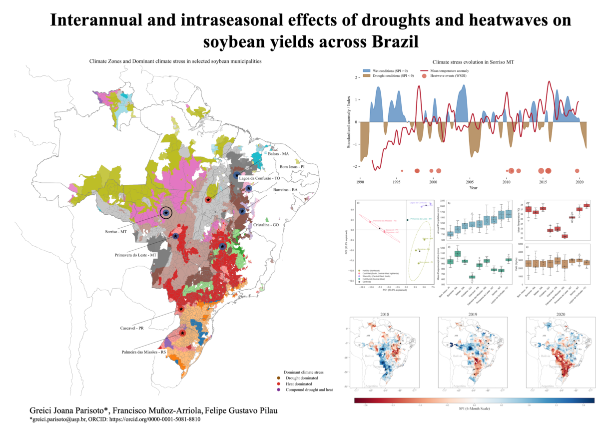
Brazil’s soybean region and studied cities (black stars). (a) Brazil’s climatic zones (Adapted from [27] and [28]. (b) spatial distribution of soybean production during the 2022/2023 crop season [31]. CZ: Climatic Zone; RS: Rio Grande do Sul; PR: Paraná; GO: Goiás; MT: Mato Grosso; BA: Bahia; TO: Tocantins; PI: Piauí; MA: Maranhão.
Figure 1.
Brazil’s soybean region and studied cities (black stars). (a) Brazil’s climatic zones (Adapted from [27] and [28]. (b) spatial distribution of soybean production during the 2022/2023 crop season [31]. CZ: Climatic Zone; RS: Rio Grande do Sul; PR: Paraná; GO: Goiás; MT: Mato Grosso; BA: Bahia; TO: Tocantins; PI: Piauí; MA: Maranhão.

Figure 2.
Flowchart of methods research.

Figure 3.
Clustering of municipalities by macroregion and agroclimatic characteristics during soybean growing seasons from 1989 to 2020. (a) Principal component analysis summarizing the multivariate structure of agroclimatic variables and yield. (b) Comparative boxplots of annual precipitation (mm). (c) Comparative boxplots of mean air temperature (°C). (d) Comparative boxplots of mean evapotranspiration (mm). (e) Comparative boxplots of soybean yield (kg ha⁻¹).

Figure 4.
Monthly Mean Precipitation (P) and Crop Evapotranspiration (ETc) with absolute values, and the soybean growing season (background colors) for each studied municipality for the period of 1989-2020 (outliers were omitted).
Figure 4.
Monthly Mean Precipitation (P) and Crop Evapotranspiration (ETc) with absolute values, and the soybean growing season (background colors) for each studied municipality for the period of 1989-2020 (outliers were omitted).

Figure 5.
Monthly mean of maximum temperature (TXx), monthly mean of minimum temperature (TNn), and the soybean growing season (background colors) for each studied municipality for the period of 1989-2020 (outliers were omitted).
Figure 5.
Monthly mean of maximum temperature (TXx), monthly mean of minimum temperature (TNn), and the soybean growing season (background colors) for each studied municipality for the period of 1989-2020 (outliers were omitted).

Figure 6.
Relative frequency distributions of daily precipitation (mm) and daily maximum temperature (°C) across the municipalities in Brazil for the period of 1989 to 2020.of soybean yield (kg ha⁻¹).
Figure 6.
Relative frequency distributions of daily precipitation (mm) and daily maximum temperature (°C) across the municipalities in Brazil for the period of 1989 to 2020.of soybean yield (kg ha⁻¹).

Figure 7.
Six-month Standardized Precipitation Index (SPI-6) for the Brazilian soybean-producing region during the period 1989–2020, calculated for the regional growing season using March as the reference month.
Figure 7.
Six-month Standardized Precipitation Index (SPI-6) for the Brazilian soybean-producing region during the period 1989–2020, calculated for the regional growing season using March as the reference month.

Figure 8.
Frequency Distribution of 6-month SPI Drought Classes and Yield Losses across Municipalities. Bars show the mean yield deviation in percent for each 6-month SPI drought class. The frequency of each class reflects the proportion of months falling within that drought category across municipalities.

Figure 9.
Frequency Distribution of 6-Month SPEI Drought Classes and Yield Losses across Municipalities. Bars show the mean yield deviation in percent for each 6-month SPEI drought class. The frequency of each class reflects the proportion of months falling within that drought category across municipalities.

Figure 10.
WSDI and Yield losses for the studied municipalities for the period of 1989-2020. WSDI: Warm Spell Duration Index.
Figure 10.
WSDI and Yield losses for the studied municipalities for the period of 1989-2020. WSDI: Warm Spell Duration Index.

Figure 11.
SPI 6-months, SPEI 6-months, Normalized Mean Temperature Anomalies, and WSDI values by region for the period of 1990 to 2020 during the soybean season.
Figure 11.
SPI 6-months, SPEI 6-months, Normalized Mean Temperature Anomalies, and WSDI values by region for the period of 1990 to 2020 during the soybean season.


Table 1.
Characteristics of municipal host sites representing each climatic zone.
| CZ | Munipality | State | Planting date window | Soil Profile | Latitude | Longitude | Elevation (m) | |
|---|---|---|---|---|---|---|---|---|
| 6801 | Palmeira das Missões | RS | 17-Sep | 31-Dec | Oxisols | -27.92 | -53.32 | 614 |
| 7801 | Cascavel | PR | 8-Sep | 31-Dec | Ultisols | -24.88 | -53.55 | 784 |
| 7601 | Cristalina | GO | 27-Sep | 31-Dec | Oxisols | -16.79 | -47.61 | 1211 |
| 7701 | Primavera do Leste | MT | 27-Sep | 31-Dec | Ultisols | -15.58 | -54.38 | 680 |
| 8701 | Sorriso | MT | 30-Sep | 25-Dec | Oxisols | -12.56 | -55.72 | 379 |
| 8401 | Barreiras | BA | 17-Oct | 31-Jan | Entisols | -12.12 | -45.03 | 474 |
| 9301 | Bom Jesus | PI | 6-Nov | 9-Feb | Entisols | -9.08 | -44.33 | 288 |
| 9401 | Balsas | MA | 17-Oct | 20-Jan | Entisols | -7.46 | -46.03 | 271 |
| 9701 | Lagoa da Confusão | TO | 8-Oct | 1-Mar | Inceptisols | -10.83 | -49.85 | 178 |
CZ: Climatic Zone; RS: Rio Grande do Sul; PR: Paraná; GO: Goiás; MT: Mato Grosso; BA: Bahia; PI: Piauí; MA: Maranhão; TO: Tocantins.
Table 2.
Classification of drought based on SPI/SPEI values. Adapted from [46].
Table 2.
Classification of drought based on SPI/SPEI values. Adapted from [46].
| SPI/SPEI | Drought class |
|---|---|
| > 1.00 | No drought/wet |
| 1.00 to -0.49 | Near normal |
| -0.50 to -0.99 | Mild drought |
| -1.00 to -1.49 | Moderate drought |
| -1.50 to -1.99 | Severe drought |
| -2.0 and less | Extreme drought |
Table 3.
Mean annual and seasonal precipitation, effective rainfall, and crop evapotranspiration values across the municipalities.
Table 3.
Mean annual and seasonal precipitation, effective rainfall, and crop evapotranspiration values across the municipalities.
| Municipality | Mean annual P (mm yr⁻¹) | Mean Season P (mm yr⁻¹) | Effective P 60% (mm yr⁻¹)1 | Mean Etc (mm yr⁻¹)2 | Effective P 60% vs Etc (mm yr⁻¹)3 |
|---|---|---|---|---|---|
| Palmeira das Missões - RS | 1,788.20 | 1,245.10 | 747 | 481.9 | 265.1 |
| Cascavel - PR | 1,746.30 | 1,126.10 | 675.6 | 443.8 | 231.8 |
| Cristalina - GO | 1,368.20 | 1,136.80 | 682.1 | 400.7 | 281.4 |
| Primavera do Leste - MT | 1,485.30 | 1,313.90 | 788.4 | 406 | 382.4 |
| Sorriso - MT | 1,664.70 | 1,486.60 | 891.9 | 362.8 | 529.1 |
| Lagoa da Confusão - TO | 1,581.40 | 1,542.80 | 925.7 | 501.4 | 424.3 |
| Barreiras - BA | 926.6 | 914.7 | 548.8 | 539.5 | 9.3 |
| Bom Jesus - PI | 814.5 | 743.3 | 446 | 498.6 | -52.6 |
| Balsas - MA | 1,082.80 | 1,058.00 | 634.8 | 465.7 | 169.1 |
1P denotes precipitation, and ETc denotes crop evapotranspiration. 2Effective P 60% represents effective precipitation estimated as 60 percent of total precipitation, following applications commonly adopted in Brazilian agroclimatic studies [57,58]. 3The surplus or deficit was determined as: (P − ETc). Positive values indicate that precipitation exceeds crop water demand, while negative values indicate a water deficit relative to ETc.
Table 4.
Soybean yield loss, expressed in thousand tonnes (kt) and as percentages (%), at the municipal level in Brazil, across crop seasons from 1989/1990 to 2020/2021.
Table 4.
Soybean yield loss, expressed in thousand tonnes (kt) and as percentages (%), at the municipal level in Brazil, across crop seasons from 1989/1990 to 2020/2021.
| Municipality | 1989/90 to 1999/00 | 2000/01 to 2010/11 | 2010/11 to 2020/21 | Total 30 Crop Seasons | ||||
|---|---|---|---|---|---|---|---|---|
| kt | % | kt | % | kt | % | kt | % | |
| Palmeira das Missões - RS | 18.8 | 2.8 | 278.1 | 13.8 | 157.8 | 6.7 | 454.6 | 9.0 |
| Cascavel - PR | 24.7 | 3.2 | 97.3 | 4.1 | 115.2 | 4.1 | 237.2 | 4.0 |
| Cristalina - GO | 13.0 | 3.1 | 228.7 | 7.5 | 222.0 | 4.0 | 463.7 | 5.2 |
| Primavera do Leste - MT | 37.8 | 2.2 | 174.0 | 2.6 | 86.8 | 1.4 | 298.6 | 2.0 |
| Sorriso - MT | 74.9 | 2.6 | 270.3 | 1.6 | 379.4 | 2.3 | 724.5 | 2.0 |
| Lagoa da Confusão - TO | 0.0 | 0.0 | 5.6 | 2.2 | 17.0 | 1.9 | 22.6 | 2.0 |
| Barreiras - BA | 66.0 | 4.3 | 227.0 | 6.7 | 265.6 | 6.3 | 558.7 | 6.1 |
| Bom Jesus - PI | 0.0 | 0.0 | 67.4 | 11.2 | 146.8 | 12.0 | 214.2 | 11.7 |
| Balsas - MA | 17.1 | 5.6 | 73.4 | 2.7 | 227.5 | 6.0 | 318.0 | 4.7 |
| Total | 252.2 | 3.0 | 1421.9 | 3.8 | 1618.1 | 3.7 | 3292.3 | 3.7 |
Table 5.
Results of the linear regression analysis between climate indices and agricultural yield indicators at the municipal level.
Table 5.
Results of the linear regression analysis between climate indices and agricultural yield indicators at the municipal level.
| Municipality | Metric | Yloss | Yr | SPEI 6M | SPI 6M | WSDI |
| Palmeira das Missões - RS | Slope | 0.031 | 55.138 | 0.019 | 0.016 | 0.014 |
| Palmeira das Missões - RS | R² value | 0.000 | 0.395 | 0.028 | 0.025 | 0.011 |
| Palmeira das Missões - RS | p-value < 0.05 | 0.898 | 0.000 | 0.118 | 0.016 | 0.106 |
| Cascavel - PR | Slope | -0.231 | 51.455 | 0.001 | 0.007 | 0.017 |
| Cascavel - PR | R² value | 0.015 | 0.642 | 0.000 | 0.004 | 0.038 |
| Cascavel - PR | p-value < 0.05 | 0.064 | 0.000 | 0.928 | 0.322 | 0.003 |
| Cristalina - GO | Slope | -0.535 | 49.919 | -0.039 | -0.034 | 0.001 |
| Cristalina - GO | R² value | 0.030 | 0.566 | 0.123 | 0.107 | 0.000 |
| Cristalina - GO | p-value < 0.05 | 0.012 | 0.000 | 0.006 | 0.000 | 0.893 |
| Primavera do Leste - MT | Slope | -0.003 | 22.562 | 0.007 | 0.007 | 0.016 |
| Primavera do Leste - MT | R² value | 0.000 | 0.514 | 0.004 | 0.005 | 0.010 |
| Primavera do Leste - MT | p-value < 0.05 | 0.986 | 0.000 | 0.553 | 0.284 | 0.118 |
| Sorriso - MT | Slope | -1.078 | 34.607 | -0.016 | -0.002 | 0.018 |
| Sorriso - MT | R² value | 0.036 | 0.661 | 0.022 | 0.000 | 0.009 |
| Sorriso - MT | p-value < 0.05 | 0.006 | 0.000 | 0.163 | 0.807 | 0.173 |
| Lagoa da Confusão - TO | Slope | -0.061 | 42.331 | 0.008 | 0.005 | 0.024 |
| Lagoa da Confusão - TO | R² value | 0.043 | 0.781 | 0.006 | 0.002 | 0.008 |
| Lagoa da Confusão - TO | p-value < 0.05 | 0.006 | 0.000 | 0.464 | 0.516 | 0.231 |
| Barreiras - BA | Slope | -0.217 | 60.532 | 0.000 | 0.003 | 0.043 |
| Barreiras - BA | R² value | 0.003 | 0.604 | 0.000 | 0.001 | 0.017 |
| Barreiras - BA | p-value < 0.05 | 0.383 | 0.000 | 0.973 | 0.699 | 0.046 |
| Bom Jesus - PI | Slope | -0.419 | 26.836 | -0.030 | -0.026 | 0.015 |
| Bom Jesus - PI | R² value | 0.040 | 0.055 | 0.067 | 0.065 | 0.003 |
| Bom Jesus - PI | p-value < 0.05 | 0.004 | 0.003 | 0.045 | 0.000 | 0.405 |
| Balsas - MA | Slope | -0.680 | 36.588 | 0.019 | 0.019 | 0.045 |
| Balsas - MA | R² value | 0.023 | 0.385 | 0.029 | 0.034 | 0.031 |
| Balsas - MA | p-value < 0.05 | 0.021 | 0.000 | 0.109 | 0.005 | 0.006 |
1SPI-6 refers to the Standardized Precipitation Index at a six-month time scale, and SPEI-6 refers to the Standardized Precipitation Evapotranspiration Index at a six-month time scale. Both indices describe medium-term moisture conditions based on precipitation and climatic water balance, respectively [20,21]. 2WSDI refers to the Warm Spell Duration Index, defined as the annual number of days belonging to warm spells according to the Expert Team on Climate Change Detection and Indices (ETCCDI) [25]. 3Yr refers to real (observed) yield, and Yloss refers to yield loss relative to a baseline or expected yield. 4R² refers to the coefficient of determination of the linear regression model. 5p-values refer to the statistical significance of the estimated slope coefficients, evaluated at conventional confidence levels.
Disclaimer/Publisher’s Note: The statements, opinions and data contained in all publications are solely those of the individual author(s) and contributor(s) and not of MDPI and/or the editor(s). MDPI and/or the editor(s) disclaim responsibility for any injury to people or property resulting from any ideas, methods, instructions or products referred to in the content. |
© 2026 by the authors. Licensee MDPI, Basel, Switzerland. This article is an open access article distributed under the terms and conditions of the Creative Commons Attribution (CC BY) license (http://creativecommons.org/licenses/by/4.0/).
Copyright: This open access article is published under a Creative Commons CC BY 4.0 license, which permit the free download, distribution, and reuse, provided that the author and preprint are cited in any reuse.


