
Submitted:
19 February 2026
Posted:
03 March 2026
You are already at the latest version
Abstract
Grazinglands store substantial soil organic carbon (SOC), yet their potential to act as net carbon (C) sinks depends on management-driven net ecosystem CO2 exchange (NEE). Process-based models capable of representing contrasting management strategies are essential for evaluating mitigation potential. However, the uncertainty inherent in model outputs is often overlooked, which can limit the reliability of predictions. Here, we apply the MEMS 3.0 model to quantify uncertainty in SOC and NEE predictions and evaluate model performance across diverse U.S. grazing ecoregions. We conducted a Bayesian calibration with observations of SOC and its fractions, and annual NEE measurements from six NEON grazing sites. Model evaluation was performed with an independent dataset collected from four experimental sites located in Oklahoma, Michigan, and Wyoming USA under prescriptive and adaptive grazing management treatments. The model performed well in predicting baseline SOC and estimating weekly ecosystem fluxes across sites. Although annual NEE estimates exhibited some discrepancies relative to flux-tower observations, ~90% of measured fluxes fell within simulated posterior predictive intervals. Moreover, the model is consistent with the flux-observations, demonstrating no significant treatment differences between prescriptive and adaptive grazing treatments at the Oklahoma and Wyoming sites. We demonstrated that MEMS 3.0 can represent SOC dynamics and ecosystem fluxes in grazinglands across contrasting climates. Our results show that neglecting uncertainty in measured and simulated fluxes can lead to misleading model-data comparisons. These findings highlights the importance of uncertainty quantification for robust interpretation of predicted grazing management outcomes and for supporting credible climate change mitigation and C accounting frameworks.
Keywords:
Bayesian calibration
; Ecosystem model
; SOM fractions
; Adaptive grazing
Highlights
- MEMS captures ecosystem SOC and NEE dynamics across diverse U.S. grazing lands
- The Bayesian framework used enabled the quantification of full model uncertainty
- Interpretation of predicted grazing outcomes can be limited without uncertainty quantification
- Quantifying model and measurement uncertainty is key for model-data comparison
1. Introduction
Climate change remains one of the greatest challenges of modern society, and drastically reducing atmospheric carbon dioxide (CO2) is needed to limit global warming below 1.5 ºC [1,2] Although agriculture has historically contributed to rising atmospheric CO2 levels [3,4], it also offers some of the most scalable opportunities for CO2 drawdown. Grazing lands are central to this potential as they represent one of the most extensive land uses on Earth covering ~25% of the planet’s ice-free surface [5] and ~67% of global agricultural land [6]. Moreover, these systems are estimated to store 10-30% of global stock of soil organic carbon (SOC), which makes their CO2 balance particularly important from a climate change perspective. Grazing management plays a crucial role in shaping whether these systems can act as net sources or sinks of CO2 [7,8], representing a major opportunity to mitigate climate change [9]. However, fully harnessing this potential requires robust tools capable of accurately simulating grazing management regimes and predicting their effects on CO2 fluxes across spatial and temporal scales. Such tools are crucial to inform sustainable land management and support climate policy and carbon (C) market frameworks [10].
Grazing management strategies strongly influence atmospheric CO2 removal primarily by regulating plant growth via defoliation. By altering the light intercepted by plants, defoliation affects the allocation of photosynthates within the plant [11,12], ultimately affecting the quantity and quality of plant inputs to the soil [13,14]. Additionally, the timing, intensity, duration, and frequency under which pastures are grazed are critical management levers that regulate plant-soil feedbacks [15]. By shaping canopy structure, regrowth dynamics, and root turnover, these levers influence both the amount of atmospheric CO2 assimilated by the vegetation and C input to the soil [15]. As a result, the optimization of these levers is expected to have major implications for CO2 drawdown, for example, through SOC accrual along the soil profile [7,15]. Decision-support tools that can represent these management levers across contrasting ecoregions, while accurately quantifying their effects on CO2 fluxes, are critical for assessing the effectiveness of grazing levers and for determining the spatial and temporal contexts in which they can deliver the most meaningful outcomes.
Process-based ecosystem models have been widely used to assess the potential outcomes of management strategies on net ecosystem CO2 exchange (NEE) [16,17,18], providing critical insights to support decision-makers toward sustainable management practices [19]. Significant advancements have enabled the inclusion of certain grazing management levers in various models, such as continuous grazing at different levels of intensity (e.g., PaSim, DayCent, DNDC, APSIM), and, more recently, non-uniform grazing distributions associated with low or no rotational grazing management systems (MEMS 3.0) [20; under review], a critical step toward accurately representing grazing management strategies. Nevertheless, the application of such models across diverse ecoregions and management strategies remains a significant challenge. This is not only due to the difficulty of accurately representing complex animal-plant-soil-microbe interactions, but mostly because reliable model predictions require high-quality measured data for model initialization and for effective calibration, evaluation, and uncertainty estimation [10]. Ideally, independent time-series datasets should be used for calibration and evaluation, which improves the robustness of model testing [21]. In practice, however, such comprehensive datasets are often scarce, especially in grazing systems, which are inherently complex due to interactions between grazing animals and plants and their feedbacks on C dynamics. Consequently, fully integrated measurements linking biomass production, SOC dynamics, and greenhouse gas fluxes are seldom available or collected simultaneously. Recently coordinated monitoring efforts across ecoregions have been established to obtain a robust assessment of grazing outcomes on ecosystem dynamics [22; under review].
Despite major advances in process-based modeling, there is limited testing in grazing systems with atmospheric flux measurements that could provide further insights into uncertainty estimates. The eddy covariance (EC) technique is a well-established approach for quantifying temporal exchanges of CO2 between land and atmosphere [23,24]. By leveraging high-frequency in situ measurements, EC estimates NEE while inherently integrating animal, vegetation, and soil processes and their responses to environmental variability and management within the measurement footprint [25]. However, most models are evaluated with SOC stock changes, which are often only detectable over long measurement timeframes (i.e., several years to a decade), creating a major limitation to model verification as well as the evaluation of management change effectiveness based on SOC remeasurement protocols, hampering the implementation for soil C markets [26]. The few studies that integrated EC and modeling rely on EC fluxes primarily to assess model performance [16,17,27,28,29] or to support model calibration and/or subsequent evaluation [18,30,31,32,33] often without the use of fully independent datasets. However, none of them have quantified the uncertainty associated with model parameters and structure on simulating either SOC or NEE fluxes. Although this does not invalidate previous applications, overlooking model uncertainty limits the robustness and interpretability of simulated ecosystem C dynamics. Addressing this knowledge gap is critical to reducing uncertainties in model estimation of atmospheric CO2 drawdown from grazing systems, which in turn enhances the reliability of model predictions of other ecosystem services (e.g., forage production, SOC storage, water dynamics, etc.), which frequently involve trade-offs relevant to management decisions.
Although process-based models are grounded in theoretical concepts and experimental evidence, they inevitably simplify reality due to incomplete representation of ecosystem processes and limited data availability. Consequently, simulations may be subject to imprecision and bias, contributing to overall model uncertainty [34]. Much of this uncertainty may arise from model parameters and structural components, which can be quantified using different methodological approaches [35,36,37,38]. Among these, Bayesian methods are widely regarded as a rigorous and transparent approach to evaluate model prediction uncertainty [39,40], especially for complex ecosystem models with numerous interacting parameters and processes [35,41]. Bayesian approaches provide a probabilistic framework in which unknown model parameters are estimated through their posterior distribution, which combines both the likelihood of the data given model parameters and the prior distribution of the model parameters [35]. The posterior distribution of the model parameters thus reflects how well the model fits the data while incorporating existing understanding of parameter values. To propagate structural uncertainty and parameter uncertainty in complex process-based models, Monte Carlo methods can be applied to quantify uncertainty in model predictions through iterative model simulation analyses [35,36,38]. The results incorporate uncertainty in model parameters and structure, providing a robust basis for deriving posterior predictive intervals in model predictions. Despite the wide range of applications of Bayesian methods across disciplines, uncertainty analysis in ecosystem modelling has remained limited to SOC simulations in croplands [34,35,36,37] and, to our knowledge, no study has yet quantified model uncertainty for SOC and NEE in grazing systems.
To address this gap, we quantified the uncertainty associated with parameters and model structure in the MEMS model version 3.0 [20; under review] by implementing a Bayesian framework using data from grassland sites in the National Ecological Observatory Network (NEON) [42]. Using a fully independent dataset from four grazing experimental sites located in Oklahoma, Michigan, and Wyoming, USA we initially tested the general model performance to predict soil temperature and soil water content, key regulators of ecosystem dynamics. Then, model evaluation was done using baseline SOC and ecosystem fluxes of treatments across grazing ecoregions by comparing model outputs with soil and EC measurements from the experimental sites. These sites span diverse ecological regions, characterized by varying vegetation types and densities, distinct climates, and a range of soil types, where livestock plays a vital role in shaping the landscape [22; under review]. We used MEMS 3.0 because it explicitly represents contrasting grazing management strategies through manipulation of key management levers and incorporates spatially non-uniform livestock distribution, which are features that are hypothesized to affect plant productivity and SOC dynamics [20; under review], and, consequently, overall NEE fluxes. Our overarching goals were to: i) assess the ability of MEMS 3.0 to represent plant dynamics across U.S. grazing ecoregions; ii) quantify the uncertainty (i.e., parameters and structure) associated with MEMS 3.0 predictions of baseline SOC and NEE of grazing lands using a Bayesian framework; and iii) evaluate the model’s performance to predict SOC in grazing lands and NEE under contrasting grazing management strategies against measurements from the experimental sites. By quantifying uncertainties in MEMS 3.0, simulating different grazing management strategies, and evaluating model predictions against independent datasets, we aim to provide a robust evidence-based approach to support researchers and decision-makers in improving C monitoring frameworks for grazing lands, which could aid in facilitating the large-scale adoption of grazing management strategies that enhance productivity while contributing to climate change mitigation.
2. Material and Methods
2.1. The MEMS Model
MEMS is a process-based ecosystem model designed to simulate soil organic matter (SOM) dynamics that integrates comprehensive ecosystem functions to represent plant growth, nutrient cycling, hydrology, and grazing management across different environments and management conditions [29]. The MEMS model represents functionally distinct and quantifiable SOC pools, namely dissolved organic carbon (DOC), particulate organic carbon (POC), and mineral associated organic carbon (MAOC). It represents much of the state-of-the-art understanding of SOC dynamics [43], including the dual-pathway SOC formation framework [44], in vivo versus ex vivo microbial processing [45], and point-of-entry dynamics [46]. Decomposition products from microbial residues and plant debris contribute to distinct SOM pools, controlled by temperature sensitivity, mineral nitrogen (N) availability, substrate C/N ratios, and water availability, reflecting site-specific biogeochemical conditions [29]. The MEMS model incorporates soil C and N cycling across a multi-layered soil profile, where DOC and mineral N move vertically along the profile, and roots contribute with fresh inputs at depth. The model captures microbial-driven N cycling processes (immobilization and mineralization) that create feedback loops influencing plant growth and SOM dynamics. Soil temperature and moisture content are modeled daily across soil layers, which allows for high-resolution representation of ecosystem responses to environmental and management changes.
The MEMS model operates on a daily timestep and requires daily weather data, soil properties, plant characteristics, and management practices as key inputs [29]. It has the capability to simulate cropping systems [47] and perennial plants [48]. Plant phenology is controlled by accumulation of thermal time and adjusted by daylength. The model dynamically adjusts green-up and dormancy for perennial plants based on soil temperature, soil water, and daylength and dynamically calculates non-structural reserves stored in the reserve organs for green up and regrowth after defoliation. In addition, reserve organs maintain a balance between minimum and maximum N content, which is translocated between the reserve organs (post-seeding and prior to dormancy) and other plant organs to support regrowth and stress conditions. Standing dead biomass is also modeled for its shading effect which impacts light interception and plant production [49]. For grazing systems, the MEMS 3.0 model [20; under review] includes plant-animal interactions to simulate the non-uniform distribution of grazing animals using a spatial explicit structure. Grazing pastures are divided into spatial units, representing discrete areas where daily animal distribution is based on a habitat suitability index (HSI) that encompasses forage quantity and quality, water proximity, shading, and physical accessibility. It also provides an option to automatically move animals with a high rotation frequency (daily in small paddocks) resulting in a more uniform grazing distribution.
2.2. Data Used for Modeling
Measurements from six grassland sites within the NEON monitoring network [42] (Figure 1) and from four experimental sites in the 3M project (Metrics, Management, and Monitoring; fully described in Stanley et al., [22; under review] were used in our study. Together, these datasets represent the most comprehensive information currently available on SOC and NEE measurements for grazing lands across the U.S. Although the datasets do not share the same set of variables, except for SOC and NEE, they were used because they are fully independent, ensuring a more robust model calibration and evaluation framework.
2.3. NEON Sites
We used data from the NEON grassland sites [Central Plains Experimental Range (CPER), Dakota Coteau Field Site (DCFS), Konza Prairie Biological Station (KONZ), Northern Great Plains Research Laboratory (NOGP), Oklahoma Agricultural Experiment Station (OAES), and Woodworth (WOOD)] for model calibration. All of these sites have been managed under cattle grazing and are instrumented with EC flux towers that continuously monitor ecosystem-atmosphere gas exchanges. To ensure high-quality model inputs, we prioritized the most reliable and consistent available data from these sites, which included MODIS gross primary productivity (GPP) estimates [50], measurements of SOC fractions (POC and MAOC) from Zhang et al. [29] along with bulk SOC and EC flux measurements from NEON [51]. Daily EC flux data were downloaded from the AmeriFlux portal [51,52,53] and processed by removing years with substantial missing data prior to calculating annual cumulative values. As part of data quality control, we excluded years in which the EC flux data showed unusually high and continuous GPP fluxes during winter, i.e., when plants are not photosynthetically active after confirming these anomalies using MODIS GPP data.
2.4. 3M Experimental Sites
The 3M project is a large collaborative grazing project aimed at assessing the ecosystem outcomes of grazing management across various U.S. grazing ecoregions. It encompasses experimental sites located in Oklahoma (OK-CR and OK-RR), Michigan (MI-LC), and Wyoming (WY-MR) [22; under review] (Figure 1). Each experimental site is constructed in a randomized block design, where each replicate block is split into two treatment plots: prescriptive (PR) and adaptive (AD) grazing management. Treatments were designed to reflect ecological outcomes of fixed PR grazing management versus flexible AD rotational grazing management. Each site had an EC flux tower installed within each treatment plot collecting data continuously. Experimental site characteristics are reported in Table 1, while a more detailed description including historical management is reported in the supplementary material. Although measurements are ongoing, this analysis of the MEMS 3.0 model includes data collected from 2022, when the experiment was started, through 2024. The data from the 3M project was used for testing key regulators of ecosystem dynamics and model evaluation.
2.4.1. Flux Tower Set-up and Measurements
Each treatment plot across the four experimental sites was equipped by Quanterra Systems Ltd, (UK) with standardized instrumentation: a sonic anemometer (Gill Windmaster), gas sampling enclosure (Quanterra 2301XX), weather station (Vaisala WXT535), four-component radiometer (Hukseflux NR01), soil probe (Meter TEROS11), and soil heat flux plate (Hukseflux HFP01) to monitor ecosystem fluxes, as well as atmospheric and soil climatic conditions. A tower was placed within a representative area of each plot chosen to minimize interference from adjacent non-target land cover types. To inform optimal placement, a flux footprint model [54] driven by ERA5 reanalysis data [55] was employed to ensure the flux source area primarily reflected the managed treatment area. The same suite of sensors was deployed across all sites. Taller towers (5.5 m) were installed at OK-CR, OK-RR, and WY-MR sites, where plots are larger, while shorter towers (3-3.7 m) were installed in MI-LC to accommodate smaller plots. Towers were designed to minimize obstruction of the radiometer’s field of view. Radiometers were positioned for optimal southern exposure, and anemometers were aligned to true north. Each tower was powered by a single solar panel positioned 10-15 m east or west of the tower to minimize airflow disturbance. Soil sensors (10 cm depth) were installed 2-3 m south of the tower to measure soil temperature, soil heat flux and water content. Sensors were calibrated as needed. Wind and gas data were collected at 10 Hz to calculate NEE fluxes, while other variables were measured at lower frequencies and aggregated accordingly. Negative NEE values, i.e., obtained when ecosystem CO2 uptake exceeds CO2 efflux, represent net C drawdown from the atmosphere into the ecosystem. Gross primary productivity and ecosystem respiration (ER) were partitioned from NEE. For detailed methodology and data processing description, please see Stanley et al. [22; under review].
2.4.2. Plant Aboveground Biomass and Leaf Area Index Measured Data
Measurements of plant biomass and leaf area index (LAI) were conducted every 28 days throughout the growing season within a 100 × 100 m grid, that was randomly established in each plot within the fetch area of the EC flux tower. The grid was divided into five transects (100 m long) spaced 20 meters apart. Biomass clippings and LAI measurements (n = 6) were collected at 5 m and 55 m along three of these transects. At each sampling, LAI was measured using a LI-COR LAI 2200, followed by aboveground biomass clipping at ground level within a 0.25 m2 circular hoop, which included both new and residual material. All plant material was oven-dried at 60 ºC for 72 hours and weighed to determine dry biomass. The period of data collection varied among sites due to differences in experiment start dates. At WY-LC, LAI was not measured because of low vegetation cover.
2.4.3. Soil Sampling and Analysis
Baseline soil samples were collected in 2022, following a triangle design [56] with 12 equilateral (1-m side) triangles per experimental plot, distributed within the fetch area of the EC tower. A hydraulic coring system (in OK-CR, OK-RR, and WY-MR; Giddings Machine Company) or percussion core (in MI-LC; AMS Inc.) were used to extract three 1-m depth cores, one per each vertex of the triangle, which were sectioned into 0-15, 15-30, 30-50, and 50-100 cm intervals and composited by triangle and depths. Soil samples were sieved first through an 8-mm and then through a 2-mm mesh to remove coarse materials such as rocks, roots, and litter. These samples were oven-dried, weighed, and quantified for correction of soil bulk density, which was determined based on soil volume and mass at each depth interval following Poeplau et al. [57]. The 2-mm soil samples were characterized for texture and pH, and fractionated by size and density [for the quantification of POC (>1.85 g cm-3), coarse heavy associated organic carbon (CHAOC; <1.85 g cm-3 and >53 μm), and MAOC (<1.85 g cm-3 and <53 μm)], following Leuthould et al. [58].
Bulk soils and physical fractions were oven-dried, ground (<0.149 mm), and analyzed for total C by dry combustion using an elemental analyzer (EA; vario Isotope Cube, Elementar). Because the MEMS 3.0 model does not simulate the CHAOC fraction and studies suggest it is more similar to MAOC than POC [58,59], we combined CHAOC with MAOC for evaluating the modeled MAOC estimates [29,60].
2.4.4. Soil Water Content Measurements
Soil water content (SWC) measurements were carried out using the TEROS 10 (METER Group, Pullman, WA) capacity sensors with factory calibration. The sensors were installed in a subset of three out of the 12 triangles. The selected triangles represented the range of topographic positions and vegetation cover at each site, ensuring that measurements captured local spatial variability. Data were recorded hourly at depths of 15, 40, and 60 cm in OK-CR, OK-RR, and MI-LC, and at 10, 20, and 30 cm in WY-MR [22; under review].
2.5. Plant Parameterization
Plant parameterization for the NEON sites was based on the initial parameter sets developed by Zhang et al. [29] using the MEMS 2.0 model. However, due to structural updates in the current model version, we re-parameterized dominant grass functional types (associated with different grass communities at each site). Plant parameters were either set to measurements from individual sites, including plant physical and chemical properties [61], or manually adjusted based on ranges reported in the literature to reproduce MODIS GPP estimates for each site.
For the experimental sites, we parameterized grasses for each site as the plant communities were different from each other. Based on the measured plant community composition [22; under review], the most representative species were identified for each location (Table 1). Literature derived values were used for some parameters while the others were manually adjusted by comparing modeled and measured plant aboveground biomass and LAI, where available.
2.6. Bayesian Framework: Model Calibration and Uncertainty Quantification
Measurements of POC, MAOC, and EC flux measurements from the six NEON grasslands sites were used for model calibration and quantification of uncertainty. Based on the global sensitivity analysis performed by Zhang et al. [29] using the NEON grassland sites, five parameters governing SOM decomposition, and therefore regulating C losses and storage, were identified as the most influential. These parameters included the potential depolymerization rate of particulate organic matter (k_POMDeplomer), the temperature sensitivity coefficient for decomposition (Coeff_TemperatureEffOnDecomp_1), the exchangeable fraction of mineral-associated organic matter (Frac_MAOMExchangeable), the decay rate constant of mineral-associated organic matter (k_MAOMDecay), and the sorption rate constant of dissolved organic matter (k_DOMSorp). These five parameters were selected for Bayesian calibration, and their prior distributions were adopted from Zhang et al. [29]. Plant parameters were excluded from the Bayesian calibration for simplicity, as our primary objective was to constrain SOC-related parameters. We assumed that the plant parameters were sufficient to represent key vegetation features in the model. Consequently, plant parameters were calibrated separately prior to the uncertainty analysis.
To calibrate the selected parameters, we implemented a DiffeRential Evolution Adaptive Metropolis (DREAM) algorithm similar to that described in Mathers et al. [36] and Zhang et al. [38]. The DREAM algorithm is a Markov chain Monte Carlo (MCMC) approach that uses multiple chains and adaptive sampling to explore complex high-dimensional parameter spaces [62]. The DREAM algorithm utilizes prior distributions on the parameter space and log likelihood values from the observed and simulated data to propose new parameter sets at each iteration. The likelihood functions were constructed to quantify the agreement between simulated and observed values of POC, MAOC, and annual NEE. As the NEON soil cores were divided into horizons of varying thickness, the measured POC and MAOC were converted to volumetric units (kg C m-3) to ensure consistency across depth intervals. Also, because these two fractions are correlated, we developed a combined likelihood function to jointly represent their covariance structure. This joint likelihood was formulated as a multivariate mixed-effects model with soil depth treated as a random effect, implemented using the “lme4” R package [63]. For annual NEE, a mixed-effects model was used with measurement year as a random effect. Assuming independence between annual NEE and the joint distribution of POC and MAOC, the overall log-likelihood for the Bayesian calibration was then computed as the sum of the log-likelihood of NEE and the joint log-likelihood of POC and MAOC. Model error (predicted value minus measured) of POC and MAOC was partitioned into variance between soil depths (σ2depth_POC and σ2depth_MAOC) and unexplained residual variance (σ2resid_SOC). Similarly, model error of annual NEE was partitioned into variance between measurement years (σ2year_NEE) and unexplained residual variance (σ2resid_NEE).
The DREAM algorithm was executed using the R package “DREAM” [64] in R version 4.4.1 [65]. Eight chains were run with a maximum of 5,000 iterations per chain. Convergence of the Markov chains was evaluated using the Gelman-Rubin diagnostic statistic (R̂) [66], with convergence assumed when R̂ ≤ 1.2, following Zhang et al. [38]. To ensure that parameter sampling reflected the stationary posterior distribution, the first 50% of iterations from each chain were discarded as burn-in, consistent with the recommendations of Vrugt et al. [62].
The last 200 parameter sets and corresponding hyperparameters (representing model error variances) from the DREAM posterior samples were used to quantify predictive uncertainty through Monte Carlo simulation following the approach of Mathers et al. [36]. This procedure propagates uncertainties in both the calibrated parameters and the hyperparameters [35], thereby accounting for variability arising from model parameters and imperfect representation of processes in its structure. For each parameter set, model simulations were conducted to generate distributions of predicted variables, from which the 2.5th and 97.5th percentiles were extracted to represent the 95% posterior predictive interval for SOC, POC, MAOC, and NEE outputs. Predictions based on the single best-performing parameter set (i.e., the maximum posterior likelihood) were also produced and are presented as the model’s best estimates for all output variables and used to generate goodness-of-fit statistics.
2.7. Model Set-up
2.7.1. NEON Sites
Simulations for the NEON sites were conducted using site specific data from Zhang et al. [29]. Soil chemical and physical attributes measured at each site were used as model inputs [61,67]. Weather data was obtained from the gridMET database [68]. Sites were assumed to be at steady state and a 1000-year spin-up was run to reach equilibrium assuming site measured SOC [61] as the reference condition. Historical fire events were scheduled according to the frequency reported in Guyette et al. [69] with each event assumed to be in the spring. Grasslands were subjected to grazing designed to mimic the impact of wild herbivores [70], during the spin-up period. Following spin-up, simulations were extended to match the temporal coverage of MODIS GPP data for each site. During this period, prescribed fire was scheduled following site-specific experimental records [71]. Because grazing management information specific to the EC tower footprint was not available, we applied the general site level grazing management (personal communication with NEON Field Science Manager Andrea C. E. Anteau) in our simulations.
2.7.2. 3M Experimental Sites
For the 3M experimental sites, model simulations were conducted for individual treatment plots at each site. Model soil inputs were based on measured soil data averaged at the plot level, along with soil hydraulic parameters estimated for each soil layer using the ROSETTA pedotransfer model [72,73]. Weather data for the pre-experimental period were obtained from the gridMET database [68]. For the experimental period, weather data collected by the EC flux towers were averaged to represent local climate conditions of each site, except WY-MR, where environmental contamination of rain gauge signals prevented reliable precipitation measurements. For this site, data from the gridMET database were used.
The simulations were conducted for three periods: non-managed native vegetation, spin-up of historical management, and the experimental period. The model was initialized by reaching a steady-state equilibrium in SOC stocks based on the native grasslands at each site through a 4000-year simulation. In this simulation, grazing intensity was set to mimic the impact of wild herbivores [70], and fire events were incorporated at frequencies specific to each ecological region [69]. For the pre-experiment spin-up period, long-term management information collected at each experimental site was used to construct the management input files. For the experimental period, specific details of the PR and AD grazing management, including the number of paddocks used for AD grazing management, stocking densities, and the dates of animal movement in and out of plots, were documented and used to define model inputs.
The MEMS 3.0 model is spatially explicit and divides the landscape into spatial units. The method developed in Zhang et al. [20; under review] was used to spatially divide the field boundary polygons into hexagons. To balance paddock size and computational efficiency, we allocated the spatial unit sizes as approximately 0.25, 0.36, 0.40, and 3.64 ha for OK-CR, OK-RR, MI-LC, and WY-MR, respectively (10 to 52 spatial units across the simulated sites). The minimal distance to drinking water source was calculated for each hexagon and used to estimate the HSI following Zhang et al. [20; under review]. This approach was based on animal movement predictions generated using a Lévy-walk model informed by GPS-collar data from Romero-Ruiz et al. [74]. As the MI-LC plots were relatively small (~4 ha), the distance to water was assumed to have a small effect on movement, and so the water index was set to 1.0 for all spatial units. The indexes for shading effect were derived using information from satellite imagery of Google Map [75] and consultations with site managers. Slope effects were not considered as elevation gradients across spatial units within each site were similar.
For consistent comparison between simulated and measured fluxes across sites, spatial units corresponding to the fetch area and exact placement of each EC flux tower (Figure 1) were selected at every experimental site.
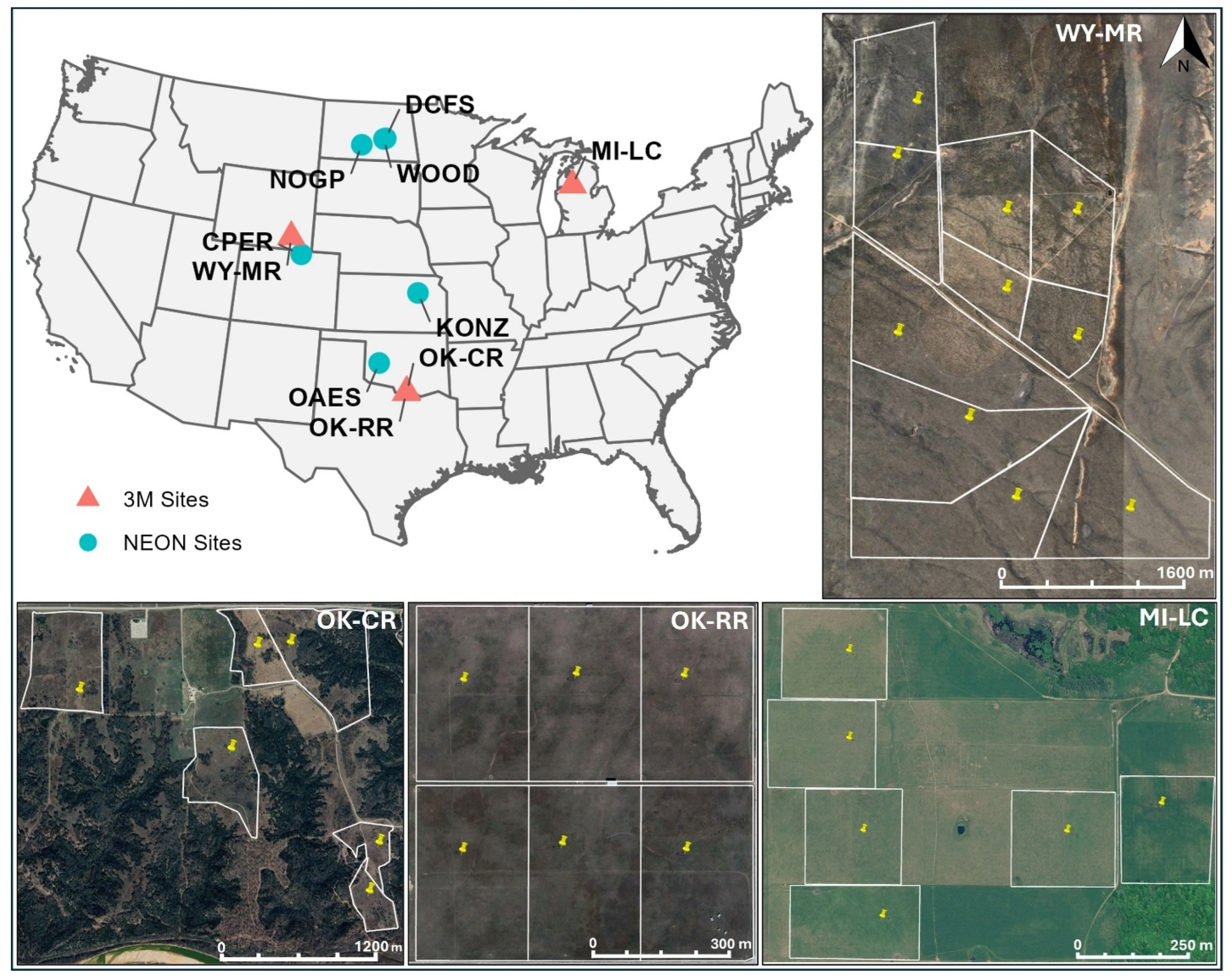
Figure 1.
Location of sites used for model calibration [National Ecological Observatory Network (NEON) sites: CPER, DCFS, KONZ, NOGP, OAES, and WOOD] and for model evaluation (3M sites: OK-CR, OK-RR, MI-LC, and WY-MR). White outlines delineate the block-level pasture areas, and pins indicate the locations of the eddy covariance flux towers at each plot across experimental sites. Satellite imagery from Google Earth Pro (© Google) accessed in November 2025.
d: index of agreement; R2: coefficient of determination; RMSE: root mean square error.
2.8. Statistical Analysis
Model calibration and performance were evaluated using the following statistical metrics:
BIAS,
index of agreement (d),
coefficient of determination (R2),
and root mean square error (RMSE),
where P refers to a predicted value i, refers to an observed value i, n is the number of observations, is the mean of predicted values, refers to a fitted value i obtained from the linear regression between observed and predicted data, and represents the mean of observed values. BIAS measures the mean tendency of simulated values to be larger or smaller than observations; values near zero indicate little systematic error; d quantifies prediction accuracy relative to observed variability and ranges from 0 to 1, with values closer to 1 indicating excellent agreement between model predictions and observations, and closer to 0 indicates no agreement at all. R2 expresses the proportion of variance in the observed data explained by a linear relationship with the predictions and varies from 0 to 1, where larger values indicate stronger association; and RMSE summarizes the average magnitude of errors, with lower values indicating more accurate simulations. Statistical metrics were calculated using daily data for soil temperature and SWC, and weekly data for NEE, GPP, and ER.
3. Results
We first evaluate plant parameterization and vegetation dynamics, followed by model performance for soil temperature and soil water content. We then present the Bayesian calibration results and subsequently provide an independent evaluation of SOC dynamics and ecosystem fluxes at the 3M experimental sites.
3.1. Plant Parameterization for the NEON and 3M Experimental Sites
Plant parameterization for the NEON grassland sites was evaluated through comparisons between simulated and MODIS-derived GPP. Across the NEON sites and multiple years, MEMS closely reproduced the seasonal dynamics and magnitude of MODIS GPP (Figure S1), as indicated by high agreement metrics (d: 0.84-0.95; R2: 0.67-0.86; Table 2). The timing of peak GPP was generally well aligned between simulated and MODIS for most sites. Nevertheless, year-specific deviations were observed, particularly at DCFS (BIAS = -6.49 g C m-2 8-day sum) and NOGP (BIAS = -6.54 g C m-2 8-day sum), where larger deviations from MODIS GPP occurred. Overall, MEMS consistently captured spatial and interannual variability in GPP across NEON grassland sites, with comparable RMSE values (5.46-11.17 g C m-2 8-day sum) among sites, indicating stable model performance.
For the 3M experimental sites, plant parameterization was based on site-level measurements of the plant community, including aboveground biomass and LAI (Table 2). Simulated and observed aboveground biomass matched relatively well across sites (d: 0.50-0.67) with the model capturing mean values adequately but showing a slight tendency to overestimate observations (BIAS: 0.04-0.88 Mg ha-1). However, the model did not reproduce the observed variability in data across sites as indicated by the low values of R2 (0.05-0.29). A similar pattern was observed for LAI (Table 2), though performance was slightly better relative to aboveground biomass (d = 0.58-0.79; R2 = 0.12-0.41), with stronger agreement at OK-CR and OK-RR, and the weakest performance at WY-MR.
3.2. Model Performance on Soil Temperature and Soil Water Content at the 3M Experimental Sites
To test the general performance of the model, we compared simulated against observed soil temperature and SWC (Table 3). The model consistently captured soil temperature changes over the measured period for all sites, as supported by the d values > 0.94 and high R2 (0.93-0.95) (Table 3). However, the model showed a slight tendency to underestimate soil temperature (BIAS: ranged from -3.84 to -1.57 ºC), especially at OK-RR, where the lowest temperature was observed (Table 2).
The model’s performance in simulating SWC had great variability across sites and depths (Table 3). Soil water content was generally slightly overestimated at 15 and 40 cm in OK-CR and MI-LC (BIAS: 0.01-0.04 cm3 cm-3), whereas it was slightly underestimated in OK-RR and WY-MR (BIAS ranged from -0.05 to -0.03 cm3 cm-3). The high values of d > 0.76 for OK-CR, OK-RR, and MI-LC suggest the model performs well at these sites, compared to WY-MR, especially at surface soil layers (d: 0.60-0.66). At deeper layer, SWC estimates were closer to observations, with small biases observed across all sites (BIAS: -0.02 to 0.01 cm3 cm-3).
3.3. Bayesian Calibration Using the NEON Sites
Bayesian calibration substantially constrained most of the parameters (Figure 2), with posterior distributions markedly narrower than the priors. However, some parameters were concentrated close to the boundaries of the ranges. The Coeff_TemperatureEffOnDecomp_1 was strongly constrained toward lower values (from 15.0 to 16 ºC), with most posterior density concentrated near the lower bound of the prior with peak at 15.3 ºC. A similar trend was observed for k_MAOMDecay, which showed a narrow posterior (0.0004 to 0.0012) centered near 0.0006. In contrast, Frac_MAOMExchangeable converged near the upper bound of the prior range. The k_POMDeplomer exhibited a narrow posterior centered on a well-defined range (0.0029 to 0.0033), whereas k_DOMSorp remained comparatively weakly constrained, exhibiting substantial posterior uncertainty (0.0101 to 0.4634).
Overall, the model showed strong agreement with measurements for SOC dynamics across soil depths, as reflected in the high values of d (0.83-0.91; Figure 3A-C). Additionally, the model explained a substantial portion of the variance in observed values (R2 = 0.62-0.83) for bulk SOC, POC, and MAOC, though it tended to underestimate these variables (BIAS ranged from -0.78 to -2.85 kg C m-3). For bulk SOC, agreement between observed and simulated values was particularly strong (d = 0.91), although the model tended to underestimate values above ~38 kg C m-3, especially in surface layers at DCFS and WOOD (Figure 3A). Across SOM fractions, POC exhibited the best performance (d = 0.93; R2 = 0.83; RMSE = 2.41 kg C m-3), while MAOC showed slightly lower predictive accuracy (R2 = 0.62) (Figure 3B-C). Similarly to bulk SOC, underestimation in POC and MAOC was mainly driven by surface soil layers at WOOD and DCFS, respectively. For annual NEE, although the model reproduced the average magnitude reasonably well (d = 0.70 and BIAS = 0.34 g C m-2), annual prediction errors remained substantial. The model explained little of the observed interannual variability (R2 = 0.30), resulting in a relatively high RMSE (106.82 g C m-2) (Figure 3D).
3.4. Model Evaluation
3.4.1. Soil Organic Carbon Dynamics at the 3M Experimental Sites
The model demonstrated high accuracy in simulating SOC dynamics along the soil profile across the experimental sites (Figure 4). For most of the sites, simulated SOC values strongly agreed with measured data, often falling within the 2.5th-97.5th percentile ranges of measured values (Figure 4A). This overall consistency is further supported by the high values of d (0.79-0.96) and R2 (0.88-0.98), and low values of BIAS and RMSE across most sites (Table 3). Nevertheless, SOC stocks were overestimated at OK-CR (BIAS: 3.54 kg C m-3) and MI-LC (BIAS: 2.90 kg C m-3), whereas they were underestimated at WY-MR (BIAS: -1.53 kg C m-3). The largest discrepancies occurred at the soil surface (<30 cm) at OK-CR, with simulated SOC approximately 1.4 times greater than measured values, in addition to simulations overestimating SOC in deeper soil layers by about twofold at MI-LC, and underestimating stocks in deeper layers by ~50% at WY-MR (Figure 4A).
Regarding SOM fractions, the model generally performed better in reproducing POC (d: 0.42-0.90) than MAOC (d: 0.25-0.72) (Figure 4B-C; Table 3), with the largest discrepancies between observed and simulated POC values occurring at WY-MR (BIAS = -3.29 kg C m-3), particularly in the 50-100 cm layer (4.21 vs. 0.12 kg C m-3; Figure 4B). For MAOC, model performance was comparatively better at WY-MR (d: 0.72, R2: 0.81, BIAS: 0.51 kg C m-3), whereas larger deviations were observed at OK-CR (BIAS: 6.01 kg C m-3) and MI-LC (BIAS: 4.39 kg C m-3). Overall, simulated MAOC values were consistently greater than measured values across sites. At OK-CR, simulated MAOC concentrations were ~30% greater than measured values across the soil profile, whereas at OK-RR they were ~2.3 times greater. At MI-LC, the overestimation increased with depth and was most pronounced below 30 cm, where simulated MAOC values averaged approximately twice the observed concentrations (Figure 4C). At WY-MR, the largest discrepancy occurred in the surface layer, with simulated MAOC ~1.3 times greater than observations. However, the variability of these sites was captured by the model as indicated by the high R2 (0.83-0.88) (Table 3). Despite these discrepancies, the model effectively captured overall SOC dynamics along the soil profile across the experimental sites (Figure 4; Table 3), as observed values consistently fell within the 95% posterior predictive intervals of modeled values. Across sites and fractions, 95% posterior predictive intervals ranged from -6.1 to 41.8 kg C m-3 for simulated, while observed 2.5th-97.5th percentile ranged from 0.3 to 41.4 kg C m-3 (Figure 4).
3.4.2. Ecosystem Fluxes at the 3M Experimental Sites
The model captured GPP temporal trends with reasonable accuracy across most experimental sites, as evidenced by the high d (0.80-0.94) and R2 values (0.68-0.82) (Table 3). However, differences in the magnitude of errors were observed across sites (RMSE: 3.70-18.8 g C m-2 week-1). At OK-RR, despite the high d value, the model showed limited ability to reproduce the EC variability (R2 = 0.52) and exhibited the greatest underestimation among sites (BIAS = -5.76 g C m-2 week-1). A GPP underestimation was observed also at OK-CR (BIAS = -2.48 g C m-2 week-1) and WY-MR (BIAS = -0.45 g C m-2 week-1), though to a lesser extent, whereas it was slightly overestimated at MI-LC (3.02 g C m-2 week-1; Table 3).
For ER, the model also reproduced temporal patterns with reasonable accuracy across experimental sites, supported by high d (0.73-0.94) and R2 (0.65-0.80). Model performance was stronger for WY-MR and OK-CR, where RMSE and BIAS were lowest, and comparatively weaker for OK-RR and MI-LC, where both metrics were higher (Table 3).
For NEE, when data were analyzed on a weekly basis (Table 3), the model reproduced the overall magnitude and direction of NEE reasonably well across most experimental sites, as indicated by the high values of d (0.68-0.80) and low BIAS (from -1.60 to 6.51 g C m-2 week-1) (Table 3). However, the relatively low R2 values (0.25-0.59) indicate that the model explained only a moderate fraction of the observed variability and was less accurate at reproducing the temporal dynamics of the EC fluxes.
Different plot-level discrepancies were observed between EC flux and simulated annual NEE across experimental sites (Figure 5). At OK-CR and MI-LC (Figure 5A, B, E, and F), the simulated annual NEE exhibited opposing patterns in the EC fluxes for most plots, irrespective of grazing management. At OK-RR and WY-MR (Figure 5C, D, G, and H), simulated and measured atmospheric flux values were more closely aligned, though overall the model tended to overestimate net C uptake at OK-RR across years and underestimate uptake at WY-MR in 2023. In 2024 the model exhibited an opposite trend in NEE at WY-MR compared to EC fluxes (~53.5 g C m-2 vs. ~ -41.9 g C m-2). Overall, the annual simulated NEE across plots for these experimental sites varied from 56.9 to 704.6 g C m-2 at MI-LC and from -84.2 to 171.4 g C m-2 at OK-CR, compared with atmospheric EC flux values of -166.7 to -16.1 g C m-2 and -137.8 to 36.8 g C m-2, respectively.
Even though simulated NEE values at the plot level differed from EC fluxes, ~90% of EC fluxes fell within the 95% posterior predictive intervals of modeled values, while one plot at OK-RR and five plots at MI-LC fell outside these limits (Figure 5). The 95% posterior predictive intervals for simulated annual NEE ranged from -498.6 to 844.9 g C m-2 across sites and years, with wider intervals in 2023 than in 2024.
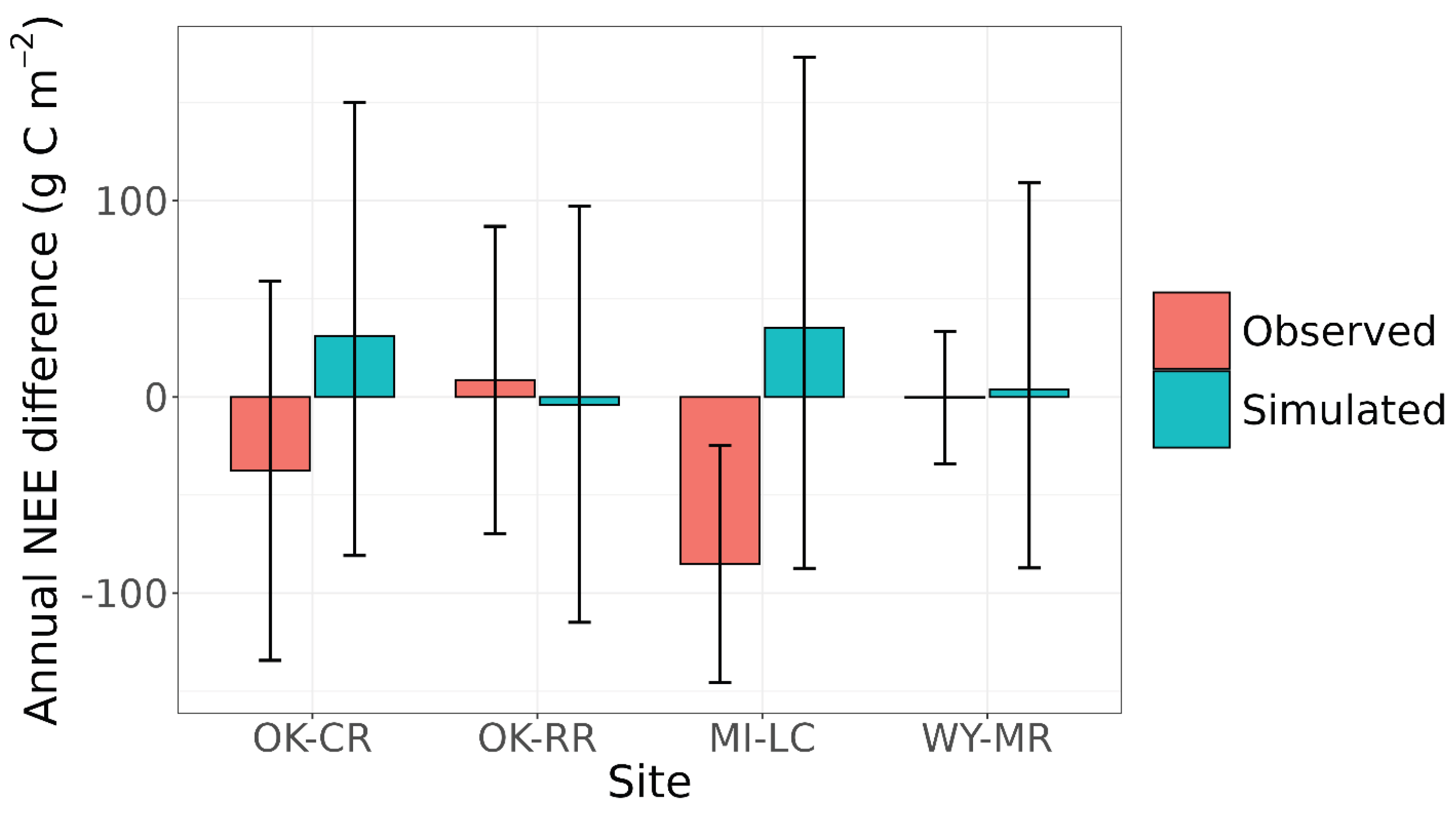
Treatment differences in annual NEE exhibited substantial variability across experimental sites, and between observed and simulated estimates (Figure 6). For the observed NEE, treatment differences were negative at OK-CR (-37.6 g C m-2), MI-LC (-85.2 g C m-2) and WY-MR (-0.3 g C m-2), whereas the difference was positive at OK-RR (8.7g C m-2). In contrast, simulated treatment differences showed an opposite pattern, with positive values at OK-CR (31.1 g C m-2) and MI-LC (35.3 g C m-2), and WY-MR (4.0 g C m-2) and negative value at OK-RR (-4.1 g C m-2). In both observed and simulated treatment differences, confidence intervals overlapped zero at all sites. The 95% confidence intervals ranged from -145.7 to 87.0 g C m-2 for EC-based NEE, while those for simulated NEE varied from -114.9 to 173.2 g C m-2.
4. Discussion
4.1. Model Performance Representing Plant Growth Dynamics at NEON and 3M Experimental Sites
Proper representation of plant growth dynamics is essential for accurately simulating SOC dynamics and ecosystem fluxes, as it governs the magnitude and timing of soil C inputs. For the NEON sites, the model reproduced the general trends of MODIS GPP relatively well, which explained most of the variability across sites and years (Table 2). However, some deviations and relatively high RMSE values indicate increased variability in model performance. This variability likely reflects limited site- and year-specific management information for the NEON sites, as the generalized management assumptions used in our simulations may have not captured the actual grazing intensity or timing. Additional discrepancies also can arise from scale mismatches between MODIS GPP and model simulations since substantial variation in soil properties and grazing pressure can occur in a single MODIS pixel but remains unrepresented in point-scale simulations (Figure S1).
Measurements of aboveground biomass and LAI at the 3M experimental sites provided valuable information for plant parameterization, as these two variables are closely related and provide a more complete understanding of vegetation growth and productivity [76]. Although MEMS 3.0 adequately captured plant biomass across experimental sites, its ability to reproduce seasonal variability was more limited, as reflected in low R2 values across sites (Table 2). For example, the model captured aboveground dynamics very well in some years under both PR and AD grazing management at MI-LC, though it was less effective in others (Figure S2). While representing dominant plant functional types, an approach commonly used in other models (e.g., DayCent [18], PaSim [77], and ORCHIDEE [16]), is often adequate for grazing systems with relatively simple vegetation structure and limited functional diversity, this simplification can limit model performance in more diverse and structurally complex landscapes. For example, a study using two versions of the ORCHIDEE model reported d values of 0.20-0.45 for aboveground biomass and 0.10-0.56 for LAI in grazed grasslands of Europe [16], substantially lower than those obtained in our study (Table 2).
In fact, in a previous study where MEMS was applied to a monoculture of bahiagrass (Paspalum notatum),[48] achieved much higher model performance (R2 = 0.72), underscoring that mixed-species communities are inherently more challenging to represent due to their diversity of traits and growth strategies. Although improving species-level representation may enhance simulations of plant dynamics and reduce uncertainty in vegetation-related outputs [78], such approaches remain challenging due to the extensive species-specific data requirements and the need substantially more complex model architectures involved [79].
4.2. Soil Temperature and Soil Water Content Dynamics at 3M Experimental Sites
Representative simulation of soil temperature and water dynamics are crucial for accurate ecosystem modeling as these factors strongly regulate plant growth, microbial activity, and the decomposition of SOM, ultimately shaping SOC dynamics and ecosystem fluxes. Our results indicated that both variables were well represented in the MEMS model (Table 3). However, soil texture and the lack of accurate simulation of snow dynamics may have influenced soil temperature and SWC, respectively.
Soil temperature was slightly underestimated, particularly during winter when observed temperatures approached or dropped below 0 ºC across sites. This bias likely reflects the simple empirical approach used to estimate soil surface temperature in our model [80], which does not explicitly resolve the surface energy balance, especially under snow-covered conditions. As a result, inaccuracies in the surface boundary condition may propagate through the soil profile, leading to systematic biases in simulated soil temperatures. These effects appear to be amplified in sandy soils, which exhibited a stronger negative bias in simulated soil temperature (Table 3), consistent with previous MEMS 2.0 results [29] and evident when comparing OK-RR and OK-CR under similar climatic conditions but contrasting soil textures. In addition, uncertainties in the spatial and temporal distribution of snow likely exacerbated discrepancies at the coldest sites (MI-LC and WY-MR), consistent with earlier DayCent model simulations of winter grassland conditions at CPER in northern Colorado [80]. Despite these limitations, the model demonstrated overall high predictive accuracy for soil temperature, in line with previous MEMS applications [29,47].
MEMS 3.0 adequately captured the temporal dynamics and magnitude of SWC across most experimental sites (Table 3), suggesting that major hydrological processes governing soil moisture, including infiltration, evaporation, and drainage, were realistically represented. Except for WY-MR, d values were relatively high and the model explained a substantial fraction of the observed variability (Table 3). The poorer performance at WY-MR likely reflects challenges in representing snow dynamics, which strongly influence water balance [81] but are not fully captured by the model. Additionally, the rock content at WY-MR, which exceeds 13% in some soil samples, may have further contributed to discrepancies in simulated and observed soil water dynamics since the ROSETTA pedotransfer model used to estimate soil hydraulic parameters does not account for rock content. Lastly, our model does not explicitly represent slope position, topographic gradients, or lateral water movement, all of which can substantially influence soil moisture dynamics and likely contributed to discrepancies between observed and simulated values.
Despite these limitations, model performance was reasonable with relatively accurate predictions across all sites and layers, with small BIAS and RMSE values indicating minimal systematic deviation (Table 3). Overall, the model performed better than previous applications of MEMS at different sites, particularly in deeper soil layers where it explained a greater portion of the observed variability [29,47] and yielded lower RMSE values [29]. Compared with PaSim simulations of Mediterranean grasslands, MEMS 3.0 produced similar d values for topsoil SWC and explained more variability at OK-CR and OK-RR, but was less accurate at MI-LC and WY-MR [82]. Relative to topsoil APSIM simulations for the Mongolian steppe, MEMS exhibited RMSE values were on average (0.06 cm3 cm-3) twice as large as those reported for APSIM [83].
4.3. Model Calibration Using the NEON Sites
The posterior distributions of the calibrated parameters showed that the Bayesian calibration reduced uncertainty in parameter ranges, indicating improved parameter identifiability (Figure 2). The posterior distributions of the two decomposition rate parameters for MAOM (“k_MAOMDecay”) and POM (“k_POMDeplomer”) were close to a bell shape, suggesting that these parameters were well constrained by the observational data. In contrast, the posterior distributions of “Coeff_TemperatureEffOnDecomp_1”, “Frac_MAOMExchangeable”, and “k_DOMSorp” were skewed toward either the lower or upper boundaries of their prior ranges. This pattern suggests potential structural limitations in the model. Specifically, such “edge-hitting” behavior often indicates that the model is attempting to compensate for simplified or omitted process representations by pushing parameters toward extreme values to minimize the residual error between observations and predictions. These patterns are also often observed in other model studies [35,36], indicating that model improvements are needed.
For annual NEE of the NEON sites, model performance may have been influenced by limited information on grazing management within the flux tower fetch areas or by incomplete representation of grassland community physiological responses to grazing and other environmental drivers. This variability was particularly evident in the predicted GPP, as in some years MEMS predictions diverged from EC estimates, which instead aligned more closely with MODIS GPP estimate [50] (Figure S1). In some other years, MEMS GPP predictions agreed well with MODIS but not with the EC flux tower (Figure S1). These results may reflect the coarse spatial resolution of MODIS (representing broader landscape conditions and management practices) contrasting with the localized footprint of EC measurements.
In addition, the quality of the EC dataset itself may have contributed to the discrepancies observed. We noticed anomalously high GPP values during winter months when they are expected to be close to 0 (Figure S1), which would result in highly negative measured NEE fluxes. Although these clearly problematic data periods were excluded from our analysis, the remaining data may still contain uncertainties arising from potential issues such as errors in gap-filling algorithms, sensor biases, or other measurement-related artifacts.
4.4. Model Performance Representing Soil Organic Carbon Dynamics at 3M Experimental Sites
Accurate representation of SOC dynamics is essential for capturing subsequent ecosystem fluxes as SOM decomposition accounts for a large fraction of ecosystem CO2 exchange. Overall, the model reproduced baseline total SOC well, but larger discrepancies emerged in the partitioning of SOM fractions (Figure 4; Table 3). The strong agreement between simulated and observed SOC at most sites (Figure 4A), reflected by high d values, indicates that the model captured the dominant controls on SOM dynamics across contrasting climates and management histories, consistent with previous MEMS applications [29,48].
Simulated SOC values generally fell within the 2.5th-97.5th percentile ranges of measurements across depths, indicating consistency with observations (Figure 4A). At the same time, site-specific BIAS values reveal systematic tendencies toward SOC overestimation at OK-CR and MI-LC and weaker underestimation at WY-MR (Table 3), suggesting that some stabilization and decomposition processes may not yet be fully represented in the model. At OK-CR, discrepancies likely reflect underrepresented surface decomposition, whereas at MI-LC, SOC overprediction at depth may indicate insufficient representation of decomposition under buffered moisture and temperature conditions. At WY-MR, missing interactions between soil inorganic C and SOC and high calcium availability, which promote C accrual through enhanced soil aggregation, co-precipitation, and mineral associations [84], as well as potential contributions from pyrogenic C [85], may have contributed to the observed tendency of underestimation.
The model also showed limitations in reproducing the observed partitioning between POC and MAOC, with POC frequently slightly underpredicted and MAOC correspondingly overpredicted (Figure 4B-C; Table 3). This imbalance likely reflects missing or simplified stabilization mechanisms, including the lack of representation of POM protection by aggregate occlusion, of mineralogy controlled organo-mineral interactions, and microbial feedbacks that are known to regulate C transfer and persistence [86]. In addition, incomplete C recovery during SOM fractionation can introduce a methodological discrepancy relative to model outputs [87], which does not account for this methodological limitation, and may further contribute to observed mismatches. Incorporating microbial-mediated and mineralogy-specific stabilization processes would likely improve the representation of SOM formation and stabilization processes [43,88], ultimately contributing to enhancing SOM fraction predictive performance.
Despite site-specific discrepancies between mean observed and simulated SOC values, the model 95% posterior predictive intervals encompassed all measurements (Figure 4), reflecting high uncertainty associated with SOC predictions. Although comparable uncertainty levels have been reported previously for cropland systems [35], explicit quantification of uncertainty in process-based SOC modeling across grazing systems remains largely unexplored, underscoring the relevance of this study. The magnitude of predictive uncertainty was, in some cases, comparable to the 2.5th-97.5th percentile ranges of the measurements themselves, highlighting the inherent spatial variability of SOC [89] and the associated challenges in constraining model simulations. These results reinforce the importance of explicitly accounting for predictive uncertainty to enable a more comprehensive interpretation of model performance, identify contexts in which predictions are most reliable, and identify potential limitations when applying SOC models across heterogeneous landscapes such as grazing lands. Addressing these uncertainties will require improved representation of context-dependent SOC controls [90,91] and detailed site-level data to better constrain parameterization and improve predictions across diverse ecoregions.
4.5. Model Performance on Gross Plant Productivity and Ecosystem Respiration at 3M Experimental Sites
The model effectively represented ecosystem dynamics across contrasting climates and grazing management strategies as indicated by the strong agreement between simulated and observed weekly cumulative GPP and ER (Table 3). These results are consistent with Chang et al. [16] who simulated seven grazed European grassland sites under diverse plant compositions and reported RMSE values ranging from 1.10 to 2.38 g C m-2 day-1 (equivalent to 7.70-16.66 g C m-2 week-1) for GPP and from 0.62 to 1.52 g C m-2 day-1 (equivalent to 4.34-10.64 g C m-2 week-1) for ER using two versions of the ORCHIDEE model. Although our analysis is based on weekly cumulative values rather than seasonal-to-annual timescales, the comparable RMSE ranges reinforce the overall good performance of our model (Table 3).
Block-level differences in simulated and EC-derived GPP reflected spatial variability in plant growth and grazing effects within the 3M experimental sites (Figure S3). During winter, EC data suggested residual plant activity while the model simulated complete dormancy, likely because the model represents only the dominant grass species and does not capture limited growth by other functional groups (e.g., cool-season species or forbs). This discrepancy was most apparent at the warmer sites (OK-CR and OK-RR) where winter conditions do not strongly constrain plant growth, whereas simulated and EC-derived GPP agreed closely at colder sites where low temperatures and snow cover limit productivity (Figure S3E-H). Simulated GPP also exhibited greater short-term variability in response to grazing events than EC estimates, particularly at MI-LC, where block-level differences were most pronounced (Figure S3E-F). This possibly reflects variability in plot-level inputs (e.g., soil texture and soil hydraulic parameters), that directly affect plant productivity. In contrast, such differences were less evident at WY-MR, possibly because EC measurements integrate fluxes over a more homogeneous landscape (e.g., soil texture). It is also important to note that flux-tower GPP is derived from measured NEE and estimated ER, which introduces additional errors [92,93] and may partially explain the mismatch between simulated and EC-derived GPP (Figure S3; Table 3). At the same time, the good agreement between simulated and MODIS-derived GPP (Figure S4) illustrates that different observation methods carry their own sources of biases, and discrepancies do not necessarily reflect model error alone.
For ER, simulated and observed values generally matched well across sites, except at OK-RR and MI-LC, where the model underestimated and overestimated ER, respectively (Table 3), although block-level simulations were more consistent with each other (Figure S5). RMSE values at these sites approached or exceeded those reported for grazed grasslands in previous modeling studies, including ORCHIDEE simulations in Europe ([16]; equivalent to 4.34-10.64 g C m-2 week-1) and DayCent simulations in semiarid grasslands in China ([94]; equivalent to 12.60 g C m-2 week-1). Most of the mismatch occurred during the growing season (Figure S5C-F), suggesting that the model did not fully capture seasonal increases in respiratory fluxes, potentially related to temporal variability in soil respiration drivers (e.g., litter and feces inputs) or biomass allocation. Because ecosystem respiration integrates multiple plant and soil components, and independent measurements of these components are lacking, isolating the exact source of this error was not possible. Furthermore, ER from EC flux towers is estimated under the assumption that nighttime NEE approximates ecosystem respiration, thus any deviation from this assumption introduces errors and may contribute to the disagreement between modelled and flux tower-derived ER [92].
4.6. Net Ecosystem Exchange at 3M Experimental Sites
While the model captured much of the observed weekly variability, minor mismatches in simulated GPP and ER accumulated over time, leading to a substantial divergence in annual NEE estimates (Table 3; Figure 5). This contrast highlights the strong sensitivity of NEE to small but persistent biases in its component fluxes (Figure 5). Because NEE represents the balance between two large and opposing fluxes (NEE = ER - GPP), even small systematic errors in either component can be amplified at longer timescales. This likely explains why model performance was consistently higher for GPP and ER than for NEE (Table 3), a pattern also observed by Kirschbaum et al. [95] when comparing atmospheric flux observations with the CenW model simulations for grazed pastures in New Zealand and France.
Capturing short-term NEE dynamics while exhibiting divergence in cumulative annual estimates has been widely documented across ecosystem models. For example, Takeda et al. [18] showed that DayCent-CABBI model reproduced the overall NEE trend over one year of measurements, but cumulative annual values diverged at most sites used for evaluation. Likewise, Chang et al. [16] reported notable mismatches between ORCHIDEE and EC flux observations across eleven European grasslands. Together, these studies reinforce that even when short-term dynamics are well captured, small biases can propagate into large annual discrepancies.
The NEE model-data mismatch may also reflect differences in instrumentation and flux-processing approaches between the NEON towers used for calibration and the Quanterra EC systems deployed at the 3M experimental sites and used for evaluation. For any EC system, installation location and instrumentation configuration coupled with anemometer coordinate rotations, lag effects, corrections for frequency response and density effects, along with varying approaches to gap-filling and quality control have potential to introduce systematic biases which are generally small on a 30-minute timescales but can accumulate over longer timescales [96,97,98]. Moreover, calibrating the model with NEON flux towers and validating with independent in-situ EC systems may have reduced predictive precision at individual experimental sites, though increased the robustness of the model evaluation [21].
Studies that calibrated models using subsets of local flux measurements, such as Falvo et al. [99] for MEMS 2.0 and Takeda et al. [18] for DayCent-CABBI, reported improved agreement between simulated and observed NEE. However, such improvements primarily reflect parameter optimization under the same environmental and management conditions used for evaluation, a practice that is frequently adopted due to data limitations but inherently limits rigorous model evaluation. By employing a strict independent calibration and evaluation Bayesian framework, our study provides a more robust assessment of model performance and uncertainty, enabling a clearer evaluation of model simulation reliability and accuracy across different ecoregions [21].
Despite discrepancies in annual NEE, modeled uncertainty generally overlapped with EC flux observations, limiting the ability to detect treatment effects even when mean differences appear to exist (Figure 5). However, this limitation is not restricted to the model, as uncertainties associated with measured EC-based annual NEE remain poorly constrained. Where they have been estimated, uncertainties ranged widely, for example from 79 to 127 g C m-2 yr-1 in a Pinus plantation [100] and from -140 to 130 g C m-2 yr-1 in Swiss grasslands [101], indicating that observational variability alone can be much larger than treatment differences.
This pattern becomes evident when examining annual NEE treatment differences for both observations and simulations (Figure 6). Although the observational confidence intervals shown here do not represent the full uncertainty associated with EC-based annual NEE, they capture the variability in NEE responses to grazing management and therefore allow a meaningful comparison with modeled uncertainty. Simulated annual mean treatment differences were often opposite in direction to the observed values. However, their confidence intervals largely overlapped across sites (Figure 6). This overlap indicates that the apparent differences in mean responses are not robust enough to support a clear divergence between modeled and observed treatment effects, but rather shows the combined effect of uncertainty in both model predictions and observations. These results underscore the importance of explicit uncertainty quantification and caution against interpreting modeled NEE predictions without consideration of associated observational uncertainty in grazing systems. This is crucial to provide a more robust foundation for model evaluation and to support decision-making based on realistic expectations of model performance across grazing lands.
Figure 6.
Annual treatment [adaptive grazing (AD) and prescriptive grazing (PR)] differences in net ecosystem exchange (NEE) derived from eddy covariance flux tower observations and model simulations across experimental sites in Oklahoma (OK-CR and OK-RR), Michigan (MI-LC), and Wyoming (WY-MR). For each experimental site, treatment differences were calculated as mean AD NEE minus mean PR NEE. Vertical bars represent the 95% confidence intervals for the mean difference in observed data between the two treatments and 95% posterior predictive intervals of the mean difference in treatments for simulations. For observed values, confidence intervals were obtained using Welch’s t-test, considering plots as replicates within each site. For simulated values, posterior predictive intervals were derived from the distribution of model outputs generated using the 200 parameter sets from the posterior of the Bayesian framework.
5. Conclusions
Studies that apply process-based models to predict ecosystem C dynamics and rigorously calibrate and evaluate them using independent datasets remain rare, particularly in grazing systems. This study advances the field by providing a Bayesian quantification of uncertainty in MEMS 3.0 predictions of both SOC and NEE, based on fully independent datasets, while jointly evaluating model performance against soil measurements and atmospheric flux observations across a broad climatic gradient in U.S. grazing lands.
Overall, MEMS 3.0 reproduced key ecosystem drivers (e.g., plant growth, soil temperature, and soil water content) across sites, providing a consistent basis for simulating SOC dynamics and ecosystem fluxes in grazing systems. However, both observed and simulated annual treatment differences in NEE exhibited large variability, posing challenges on accurately detecting grazing management effects.
Reducing uncertainty in model-based assessments of grazing systems will require advances on both observational and modeling fronts. Improved harmonization and longer time series of EC flux measurements will strengthen model calibration and evaluation. Also, explicitly accounting for uncertainty associated with EC flux measurements would provide a more robust basis for model-data comparisons. For the NEON sites, more detailed management records and plant measurements (e.g., biomass and LAI) within EC flux tower footprints would be particularly valuable for better constraining plant parameterization and linking EC fluxes to ecosystem changes.
Our study emphasizes the importance of explicitly accounting for modeling uncertainty as it provides a more robust framework for interpreting model results and sets realistic expectations regarding the strengths and limitations of process-based models applied to grazing systems. Ultimately, this is essential for evaluating grazing as a climate mitigation strategy and for developing credible C accounting, while simultaneously balancing livestock production goals.
Author Contributions
Rafael S. Santos: Data curation, Formal analysis, Investigation, Methodology, Software, Visualization, Writing - original draft, Writing - review & editing. Emma K. Hamilton: Data curation, Formal analysis, Investigation, Methodology, Software, Writing - review & editing. Paige L. Stanley: Methodology, Writing - review & editing. Robert Clement: Methodology, Writing - review & editing. Rebecca Mitchell: Methodology, Writing – review & editing. Hao Yang: Data curation, Writing - review & editing. Lauren Hoskovec: Methodology, Writing - review & editing. Isabella C. F. Maciel: Data curation, Methodology, Writing - review & editing. Jason Rowntree: Methodology, Funding acquisition, Project administration, Writing - review & editing. John D. Scasta: Data curation, Methodology, Writing - review & editing. Alejandro Romero-Ruiz: Methodology, Writing - review & editing. Steven M. Ogle: Methodology, Writing - review & editing. M. Francesca Cotrufo: Conceptualization, Investigation, Methodology, Funding acquisition, Project administration, Supervision, Writing - original draft, Writing - review & editing. Yao Zhang: Conceptualization, Data curation, Formal analysis, Investigation, Methodology, Software, Project administration, Supervision, Visualization, Writing - original draft, Writing - review & editing.
Data Availability Statement
Data will be made available on request.
Acknowledgments
This research was supported by the Foundation for Food and Agriculture Research (FFAR grant number: DSnew-0000000028), the Noble Institute, Greenacres Foundation, and Butcherbox, the United States Department of Agriculture (USDA agreement number NR233A750004G050), and the Shell International Exploration and Production Inc. (contract n. CW517568). The content of this publication is solely the responsibility of the authors and does not necessarily represent the official views of our funders. We thank NEON Field Science Manager Andrea C. E. Anteau for providing site management information. We thank Erica L. Patterson for soil sampling. We thank Alexandria Kuhl, Glenn O’Neil, and Jeremiah Asher for providing soil water data. We thank Guilhermo F. S. Congio, Hugh Aljoe, Jeff J. Goodwin, João P. Sacramento, Lautaro Garcia, Nicole M. Nimlos, and Timm Gergeni for assistance with site management information. We thank staff from Lake City Research Station, Noble Research institute, and McGuire Ranch in assistance with experimental sites maintenance and cattle management.
Conflicts of Interest
Yao Zhang, Rafael S. Santos, Emma K. Hamilton, Steven Ogle, and M. Francesca Cotrufo receive a portion of the licensing fees associated with the MEMS model. All other authors declare no known competing financial interests or personal relationships that could have influenced the work reported in this paper.
References
- Panmao, Z. Climate Change 2022: Mitigation of Climate Change; Contribution of Working Group III to the Sixth Assessment Report of the Intergovernmental Panel on Climate Change; IPCC Sixth Assessment Report; IPCC: Geneva, Switzerland, 2022. [CrossRef]
- Zhang, C.; Dong, Q.; Chu, H.; Shi, J.; Li, S.; Wang, Y.; Yang, X. Grassland Community Composition Response to Grazing Intensity Under Different Grazing Regimes. Rangel. Ecol. Manag. 2018, 71, 196–204. [CrossRef]
- Ren, S.; Terrer, C.; Li, J.; Cao, Y.; Yang, S.; Liu, D. Historical impacts of grazing on carbon stocks and climate mitigation opportunities. Nat. Clim. Chang. 2024, 14, 380–386. [CrossRef]
- Sanderman, J.; Hengl, T.; Fiske, G.J. Soil carbon debt of 12,000 years of human land use. Proc. Natl. Acad. Sci. 2017, 114, 9575–9580. [CrossRef]
- Lal, R. Digging deeper: A holistic perspective of factors affecting soil organic carbon sequestration in agroecosystems. Glob. Chang. Biol. 2018, 24, 3285–3301. [CrossRef]
- FAO. Land statistics 2001–2022 – Global, regional and country trends. FAOSTAT Analytical Briefs, No. 88. Rome. [Internet]. . Available from: https://openknowledge.fao.org/handle/20.500.14283/cd1484en.
- Bai, Y.; Cotrufo, M.F. Grassland soil carbon sequestration: Current understanding, challenges, and solutions. Science 2022, 377, 603–608. [CrossRef]
- McSherry, M.E.; Ritchie, M.E. Effects of grazing on grassland soil carbon: a global review. Glob. Chang. Biol. 2013, 19, 1347–1357. [CrossRef]
- Paustian, K.; Lehmann, J.; Ogle, S.; Reay, D.; Robertson, G.P.; Smith, P. Climate-smart soils. Nature 2016, 532, 49–57. [CrossRef]
- Bradford, M.A.; Kuebbing, S.E.; Polussa, A.; Sanderman, J.; Oldfield, E.E. Upstream data need to prove soil carbon as a climate solution. Nat. Clim. Chang. 2025, 15, 1013–1016. [CrossRef]
- Dong M, de Kroon H. Plasticity in Morphology and Biomass Allocation in Cynodon dactylon, a Grass Species Forming Stolons and Rhizomes. Oikos [Internet]. 70(1), 99 (1994). Available from: https://www.jstor.org/stable/3545704?origin=crossref.
- Turner, C.L.; Seastedt, T.R.; Dyer, M.I. Maximization of Aboveground Grassland Production: The Role of Defoliation Frequency, Intensity, and History. Ecol. Appl. 1993, 3, 175–186. [CrossRef]
- Milchunas, D.G.; Varnamkhasti, A.S.; Lauenroth, W.K.; Goetz, H. Forage quality in relation to long-term grazing history, current-year defoliation, and water resource. Oecologia 1995, 101, 366–374. [CrossRef]
- Pavlů, V.; Hejcman, M.; Pavlů, L.; Gaisler, J.; Nežerková, P. Effect of continuous grazing on forage quality, quantity and animal performance. Agric. Ecosyst. Environ. 2006, 113, 349–355. [CrossRef]
- Stanley, P.L.; Wilson, C.; Patterson, E.; Machmuller, M.B.; Cotrufo, M.F. Ruminating on soil carbon: Applying current understanding to inform grazing management. Glob. Chang. Biol. 2024, 30, e17223. [CrossRef]
- Chang, J.F.; Viovy, N.; Vuichard, N.; Ciais, P.; Wang, T.; Cozic, A.; Lardy, R.; Graux, A.-I.; Klumpp, K.; Martin, R.; et al. Incorporating grassland management in ORCHIDEE: model description and evaluation at 11 eddy-covariance sites in Europe. Geosci. Model Dev. 2013, 6, 2165–2181. [CrossRef]
- Lawton, D.; Leahy, P.; Kiely, G.; Byrne, K.A.; Calanca, P. Modeling of net ecosystem exchange and its components for a humid grassland ecosystem. J. Geophys. Res. Biogeosciences 2006, 111. [CrossRef]
- Takeda, N.; Rowlings, D.; Parton, W.; Grace, L.; Day, K.; Nguyen, T.; Grace, P. Soil carbon sequestration potential in subtropical grasslands estimated by DayCent-CABBI. Soil Sci. Soc. Am. J. 2025, 89. [CrossRef]
- E Campbell, E.; Paustian, K. Current developments in soil organic matter modeling and the expansion of model applications: a review. Environ. Res. Lett. 2015, 10, 123004. [CrossRef]
- Zhang Y, Santos RS, Hamilton EK, et al. Modeling the Effects of Livestock Rotation Frequency on Forage Production and Soil Carbon Using a Spatially Explicit Grazing Distribution [Internet]. (2026). Available from: https://www.preprints.org/manuscript/202602.0923/v1.
- Le Noë, J.; Manzoni, S.; Abramoff, R.; Bölscher, T.; Bruni, E.; Cardinael, R.; Ciais, P.; Chenu, C.; Clivot, H.; Derrien, D.; et al. Soil organic carbon models need independent time-series validation for reliable prediction. Commun. Earth Environ. 2023, 4, 1–8. [CrossRef]
- Stanley P, Kuhl A, Rowntree J, Maciel I. Merging Rigor and Relevance in Grazingland Research: A Comprehensive Social-Ecological Monitoring Approach. Under review. (2026).
- Baldocchi, D. Measuring fluxes of trace gases and energy between ecosystems and the atmosphere – the state and future of the eddy covariance method. Glob. Chang. Biol. 2014, 20, 3600–3609. [CrossRef]
- Eugster, W.; Merbold, L. Eddy covariance for quantifying trace gas fluxes from soils. SOIL 2015, 1, 187–205. [CrossRef]
- Baldocchi, D.D. How eddy covariance flux measurements have contributed to our understanding of Global Change Biology. Glob. Chang. Biol. 2019, 26, 242–260. [CrossRef]
- Oldfield, E.E.; Lavallee, J.M.; Blesh, J.; Bradford, M.A.; Cameron-Harp, M.; Cotrufo, M.F.; Eagle, A.J.; Eash, L.; Even, R.J.; Kuebbing, S.E.; et al. Greenhouse gas mitigation on croplands: clarifying the debate on knowns, unknowns and risks to move forward with effective management interventions. Carbon Manag. 2024, 15. [CrossRef]
- Gottschalk, P.; Wattenbach, M.; Neftel, A.; Fuhrer, J.; Jones, M.; Lanigan, G.; Davis, P.; Campbell, C.; Soussana, J.-F.; Smith, P. The role of measurement uncertainties for the simulation of grassland net ecosystem exchange (NEE) in Europe. Agric. Ecosyst. Environ. 2007, 121, 175–185. [CrossRef]
- Vuichard, N.; Soussana, J.; Ciais, P.; Viovy, N.; Ammann, C.; Calanca, P.; Clifton-Brown, J.; Fuhrer, J.; Jones, M.; Martin, C. Estimating the greenhouse gas fluxes of European grasslands with a process-based model: 1. Model evaluation from in situ measurements. Glob. Biogeochem. Cycles 2007, 21. [CrossRef]
- Zhang, Y.; Lavallee, J.M.; Robertson, A.D.; Even, R.; Ogle, S.M.; Paustian, K.; Cotrufo, M.F. Simulating measurable ecosystem carbon and nitrogen dynamics with the mechanistically defined MEMS 2.0 model. Biogeosciences 2021, 18, 3147–3171. [CrossRef]
- Hu, T.; Malone, S.L.; Rumpel, C.; Chabbi, A. Maximizing soil organic carbon stocks through optimal ploughing and renewal strategies in (Ley) grassland. Commun. Earth Environ. 2024, 5, 1–10. [CrossRef]
- Puche, N.; Senapati, N.; Flechard, C.R.; Klumpp, K.; Kirschbaum, M.U.; Chabbi, A. Modeling Carbon and Water Fluxes of Managed Grasslands: Comparing Flux Variability and Net Carbon Budgets between Grazed and Mowed Systems. Agronomy 2019, 9, 183. [CrossRef]
- Sándor, R.; Barcza, Z.; Hidy, D.; Lellei-Kovács, E.; Ma, S.; Bellocchi, G. Modelling of grassland fluxes in Europe: Evaluation of two biogeochemical models. Agric. Ecosyst. Environ. 2016, 215, 1–19. [CrossRef]
- Thentu, T.L.; Forster, D.; Li, Y.; Virkajärvi, P.; Harrison, M.T.; Mitra, B.; Deng, J.; Korhonen, P.; Shurpali, N. DNDC modelling of greenhouse gas exchange from a boreal legume grassland under organic and mineral nitrogen management. J. Environ. Manag. 2025, 390, 126344. [CrossRef]
- Ogle, S.M.; Breidt, F.J.; Easter, M.; Williams, S.; Killian, K.; Paustian, K. Scale and uncertainty in modeled soil organic carbon stock changes for US croplands using a process-based model. Glob. Chang. Biol. 2010, 16, 810–822. [CrossRef]
- Gurung, R.B.; Ogle, S.M.; Breidt, F.J.; Williams, S.A.; Parton, W.J. Bayesian calibration of the DayCent ecosystem model to simulate soil organic carbon dynamics and reduce model uncertainty. Geoderma 2020, 376. [CrossRef]
- Mathers, C.; Black, C.K.; Segal, B.D.; Gurung, R.B.; Zhang, Y.; Easter, M.J.; Williams, S.; Motew, M.; Campbell, E.E.; Brummitt, C.D.; et al. Validating DayCent-CR for cropland soil carbon offset reporting at a national scale. Geoderma 2023, 438. [CrossRef]
- Ogle, S.M.; Breidt, F.J.; Easter, M.; Williams, S.; Paustian, K. An empirically based approach for estimating uncertainty associated with modelling carbon sequestration in soils. Ecol. Model. 2007, 205, 453–463. [CrossRef]
- Zhang, Y.; Arabi, M.; Paustian, K. Analysis of parameter uncertainty in model simulations of irrigated and rainfed agroecosystems. Environ. Model. Softw. 2020, 126. [CrossRef]
- van Oijen, M. Bayesian Methods for Quantifying and Reducing Uncertainty and Error in Forest Models. Curr. For. Rep. 2017, 3, 269–280. [CrossRef]
- Van Oijen, M.; Rougier, J.; Smith, R. Bayesian calibration of process-based forest models: bridging the gap between models and data. Tree Physiol. 2005, 25, 915–927. [CrossRef]
- Lu, D.; Ricciuto, D.; Walker, A.; Safta, C.; Munger, W. Bayesian calibration of terrestrial ecosystem models: a study of advanced Markov chain Monte Carlo methods. Biogeosciences 2017, 14, 4295–4314. [CrossRef]
- Hinckley, E.S.; Bonan, G.B.; Bowen, G.J.; Colman, B.P.; Duffy, P.A.; Goodale, C.L.; Houlton, B.Z.; Marín-Spiotta, E.; Ogle, K.; Ollinger, S.V.; et al. The soil and plant biogeochemistry sampling design for The National Ecological Observatory Network. Ecosphere 2016, 7, e01234. [CrossRef]
- Rocci, K.S.; Cotrufo, M.F.; Ernakovich, J.; Foster, E.; Frey, S.; Georgiou, K.; Grandy, A.S.; Malhotra, A.; Reich, P.B.; Schlerman, E.P.; et al. Bridging 20 Years of Soil Organic Matter Frameworks: Empirical Support, Model Representation, and Next Steps. J. Geophys. Res. Biogeosciences 2024, 129. [CrossRef]
- Cotrufo, M.F.; Soong, J.L.; Horton, A.J.; Campbell, E.E.; Haddix, M.L.; Wall, D.H.; Parton, W.J. Formation of soil organic matter via biochemical and physical pathways of litter mass loss. Nat. Geosci. 2015, 8, 776–779. [CrossRef]
- Liang, C.; Schimel, J.P.; Jastrow, J.D. The importance of anabolism in microbial control over soil carbon storage. Nat. Microbiol. 2017, 2, 17105. [CrossRef]
- Sokol, N.W.; Sanderman, J.; Bradford, M.A. Pathways of mineral-associated soil organic matter formation: Integrating the role of plant carbon source, chemistry, and point of entry. Glob. Chang. Biol. 2018, 25, 12–24. [CrossRef]
- Zhang, Y.; King, A.E.; Hamilton, E.; Cotrufo, M.F. Representing cropping systems with the MEMS 2 ecosystem model. Agron. J. 2024, 116, 2328–2345. [CrossRef]
- Santos, R.S.; Hamilton, E.K.; Stanley, P.L.; Paustian, K.; Cotrufo, M.F.; Zhang, Y. Simulating adaptive grazing management on soil organic carbon in the Southeast U.S.A. using MEMS 2. J. Environ. Manag. 2024, 365, 121657. [CrossRef]
- Santos, R.S.; Hamilton, E.K.; Stanley, P.L.; Paustian, K.; Cotrufo, M.F.; Zhang, Y. Simulating adaptive grazing management on soil organic carbon in the Southeast U.S.A. using MEMS 2. J. Environ. Manag. 2024, 365, 121657. [CrossRef]
- Running S, Mu Q, Zhao M. MODIS/Terra Gross Primary Productivity 8-Day L4 Global 500m SIN Grid V061 [Data set]. NASA Land Processes Distributed Active Archive Center. (2021).
- NEON. NEON Eddy-Covariance Tower Data (DP4.00200.001) for sites US-xDC, US-xAE, US-xCP, US-xKZ, US-xNG, and US-xWD. Dataset accessed via AmeriFlux Portal - Lawrence Berkeley National Laboratory (https://ameriflux.lbl.gov). [Internet]. . Available from: https://ameriflux.lbl.gov.
- Novick, K.; Biederman, J.; Desai, A.; Litvak, M.; Moore, D.; Scott, R.; Torn, M. The AmeriFlux network: A coalition of the willing. Agric. For. Meteorol. 2018, 249, 444–456. [CrossRef]
- Pastorello G, Trotta C, Canfora E, et al. The FLUXNET2015 dataset and the ONEFlux processing pipeline for eddy covariance data. Sci. Data [Internet]. 7(1), 225 (2020). Available from: https://www.nature.com/articles/s41597-020-0534-3.
- Kormann, R.; Meixner, F.X. An Analytical Footprint Model For Non-Neutral Stratification. Boundary-Layer Meteorol. 2001, 99, 207–224. [CrossRef]
- Hersbach, H.; Bell, B.; Berrisford, P.; Hirahara, S.; Horányi, A.; Muñoz-Sabater, J.; Nicolas, J.; Peubey, C.; Radu, R.; Schepers, D.; et al. The ERA5 global reanalysis. Q. J. R. Meteorol. Soc. 2020, 146, 1999–2049. [CrossRef]
- Spencer, S.; Ogle, S.M.; Breidt, F.J.; Goebel, J.J.; Paustian, K. Designing a national soil carbon monitoring network to support climate change policy: a case example for US agricultural lands. Greenh. Gas Meas. Manag. 2011, 1, 167–178. [CrossRef]
- Poeplau, C.; Vos, C.; Don, A. Soil organic carbon stocks are systematically overestimated by misuse of the parameters bulk density and rock fragment content. SOIL 2017, 3, 61–66. [CrossRef]
- Leuthold SJ, Haddix ML, Lavallee J, Cotrufo MF. Physical fractionation techniques [Internet]. In: Reference Module in Earth Systems and Environmental Sciences, Elsevier, 1–13 (2022). Available from: https://linkinghub.elsevier.com/retrieve/pii/B9780128229743000677.
- Samson, M.; Chantigny, M.H.; Vanasse, A.; Menasseri-Aubry, S.; Angers, D.A. Coarse mineral-associated organic matter is a pivotal fraction for SOM formation and is sensitive to the quality of organic inputs. Soil Biol. Biochem. 2020, 149. [CrossRef]
- Cotrufo, M.F.; Haddix, M.L.; Mullen, J.L.; Zhang, Y.; McKay, J.K. Deepening Root Inputs: Potential Soil Carbon Accrual From Breeding for Deeper Rooted Maize. Glob. Chang. Biol. 2024, 30, e17591. [CrossRef]
- NEON. Soil physical and chemical properties, Megapit (DP1.00096.001), RELEASE-2025. Dataset accessed from https://data.neonscience.org/data-products/DP1.00096.001/RELEASE-2025 on October 10, 2025. [Internet]. Available from: https://data.neonscience.org/data-products/DP1.00096.001/RELEASE-2025. [CrossRef]
- Vrugt JA, Ter Braak CJF. DREAM (D) : an adaptive Markov Chain Monte Carlo simulation algorithm to solve discrete, noncontinuous, and combinatorial posterior parameter estimation problems. Hydrol. Earth Syst. Sci. [Internet]. 15(12), 3701–3713 (2011). Available from: https://hess.copernicus.org/articles/15/3701/2011/.
- Bates D, Mächler M, Bolker B, Walker S. Fitting Linear Mixed-Effects Models Using lme4. J. Stat. Softw. [Internet]. 67(1) (2015). Available from: http://www.jstatsoft.org/v67/i01/.
- Guillaume J, Andrews F. dream: DiffeRential Evolution Adaptive Metropolis. R package version 0.4-2. URL http://CRAN.R-project.org/package=dream [Internet]. CRAN: Contributed Packages (2012). Available from: http://CRAN.R-project.org/package=dream.
- R Core Team. R: A Language and Environment for Statistical Computing_. R Foundation for Statistical Computing. at https://www.r-project.org/ (2024).
- Gelman A, Rubin DB. Inference from Iterative Simulation Using Multiple Sequences. Statistical Science [Internet]. 7(4) (1992). Available from: https://projecteuclid.org/journals/statistical-science/volume-7/issue-4/Inference-from-Iterative-Simulation-Using-Multiple-Sequences/10.1214/ss/1177011136.full.
- NEON. Soil physical and chemical properties, distributed initial characterization (DP1.10047.001), RELEASE-2025. Dataset accessed from https://data.neonscience.org/data-products/DP1.10047.001/RELEASE-2025 on October 10, 2025. [CrossRef]
- Abatzoglou, J.T. Development of gridded surface meteorological data for ecological applications and modelling. Int. J. Climatol. 2013, 33, 121–131. [CrossRef]
- Guyette, R.P.; Stambaugh, M.C.; Dey, D.C.; Muzika, R.-M. Predicting Fire Frequency with Chemistry and Climate. Ecosystems 2012, 15, 322–335. [CrossRef]
- Knapp, A.K.; Briggs, J.M.; Collins, S.L.; Hartnett, D.C.; Johnson, L.C.; Towne, E.G. The Keystone Role of Bison in North American Tallgrass PrairieBison increase habitat heterogeneity and alter a broad array of plant, community, and ecosystem processes. BioScience 1999, 49, 39–50. [CrossRef]
- NEON. Site management and event reporting (DP1.10111.001), RELEASE-2025. Dataset accessed from https://data.neonscience.org/data-products/DP1.10111.001/RELEASE-2025 on October 10, 2025. [CrossRef]
- Beaudette, D.; Skovlin, J.; Roecker, S.; Brown, A. soilDB: Soil Database Interface. R package version 2.8.13. (2025). Available from: https://CRAN.R-project.org/package=soilDB.
- Schaap, M.G.; Leij, F.J.; van Genuchten, M.T. rosetta: a computer program for estimating soil hydraulic parameters with hierarchical pedotransfer functions. J. Hydrol. 2001, 251, 163–176. [CrossRef]
- Romero-Ruiz A, Rivero MJ, Milne A, et al. Grazing livestock move by Lévy walks: Implications for soil health and environment. J. Environ. Manage. 345 (2023).
- Google. Google Maps Satellite Imagery [Data set]. [Internet]. (2025). Available from: https://www.google.com/maps.
- M., S.E.; J., J.; B., S.; M., D.; C., K. Above-ground resource use increases with plant species richness in experimental grassland ecosystems. Funct. Ecol. 2000, 14, 326–337. [CrossRef]
- Riedo, M.; Grub, A.; Rosset, M.; Fuhrer, J. A pasture simulation model for dry matter production, and fluxes of carbon, nitrogen, water and energy. Ecol. Model. 1998, 105, 141–183. [CrossRef]
- Van Oijen, M.; Barcza, Z.; Confalonieri, R.; Korhonen, P.; Kröel-Dulay, G.; Lellei-Kovács, E.; Louarn, G.; Louault, F.; Martin, R.; Moulin, T.; et al. Incorporating Biodiversity into Biogeochemistry Models to Improve Prediction of Ecosystem Services in Temperate Grasslands: Review and Roadmap. Agronomy 2020, 10, 259. [CrossRef]
- Kipling, R.P.; Virkajärvi, P.; Breitsameter, L.; Curnel, Y.; De Swaef, T.; Gustavsson, A.-M.; Hennart, S.; Höglind, M.; Järvenranta, K.; Minet, J.; et al. Key challenges and priorities for modelling European grasslands under climate change. Sci. Total. Environ. 2016, 566-567, 851–864. [CrossRef]
- Parton, W.J.; Hartman, M.; Ojima, D.; Schimel, D. DAYCENT and its land surface submodel: description and testing. Glob. Planet. Chang. 1998, 19, 35–48. [CrossRef]
- Maurer, G.E.; Bowling, D.R. Seasonal snowpack characteristics influence soil temperature and water content at multiple scales in interior western U.S. mountain ecosystems. Water Resour. Res. 2014, 50, 5216–5234. [CrossRef]
- Pulina, A.; Lai, R.; Salis, L.; Seddaiu, G.; Roggero, P.P.; Bellocchi, G. Modelling pasture production and soil temperature, water and carbon fluxes in Mediterranean grassland systems with the Pasture Simulation model. Grass Forage Sci. 2017, 73, 272–283. [CrossRef]
- Wu, L.; Liu, H.; Liang, B.; Zhu, X.; Cao, J.; Wang, Q.; Jiang, L.; Cressey, E.L.; Quine, T.A. A process-based model reveals the restoration gap of degraded grasslands in Inner Mongolian steppe. Sci. Total. Environ. 2022, 806, 151324. [CrossRef]
- Rowley, M.C.; Grand, S.; Verrecchia, É.P. Calcium-mediated stabilisation of soil organic carbon. Biogeochemistry 2018, 137, 27–49. [CrossRef]
- Glaser, B.; Amelung, W. Pyrogenic carbon in native grassland soils along a climosequence in North America. Glob. Biogeochem. Cycles 2003, 17. [CrossRef]
- Cotrufo, M.F.; Lavallee, J.M. Soil organic matter formation, persistence, and functioning: A synthesis of current understanding to inform its conservation and regeneration. In: Advances in Agronomy, Academic Press Inc., 1–66 (2022).
- Poeplau, C.; Don, A.; Six, J.; Kaiser, M.; Benbi, D.; Chenu, C.; Cotrufo, M.F.; Derrien, D.; Gioacchini, P.; Grand, S.; et al. Isolating organic carbon fractions with varying turnover rates in temperate agricultural soils – A comprehensive method comparison. Soil Biol. Biochem. 2018, 125, 10–26. [CrossRef]
- Manzoni, S.; Schimel, J.P. Advances in modelling soil microbial dynamics. Soil Biol. Biochem. 2024, 197. [CrossRef]
- Stanley, P.; Spertus, J.; Chiartas, J.; Stark, P.B.; Bowles, T. Valid inferences about soil carbon in heterogeneous landscapes. Geoderma 2023, 430. [CrossRef]
- Hansen, P.M.; Even, R.; King, A.E.; Lavallee, J.; Schipanski, M.; Cotrufo, M.F. Distinct, direct and climate-mediated environmental controls on global particulate and mineral-associated organic carbon storage. Glob. Chang. Biol. 2023, 30, e17080. [CrossRef]
- Lavallee, J.M.; Haddix, M.L.; Swan, A.; Hoover, J.D.; Cotrufo, M.F. Using aridity as an overarching factor to advance understanding of soil organic carbon storage at the continental scale. Biogeochemistry 2025, 168, 1–25. [CrossRef]
- Oikawa, P.; Sturtevant, C.; Knox, S.; Verfaillie, J.; Huang, Y.; Baldocchi, D. Revisiting the partitioning of net ecosystem exchange of CO2 into photosynthesis and respiration with simultaneous flux measurements of 13CO2 and CO2, soil respiration and a biophysical model, CANVEG. Agric. For. Meteorol. 2017, 234-235, 149–163. [CrossRef]
- Reichstein, M.; Falge, E.; Baldocchi, D.; Papale, D.; Aubinet, M.; Berbigier, P.; Bernhofer, C.; Buchmann, N.; Gilmanov, T.; Granier, A.; et al. On the separation of net ecosystem exchange into assimilation and ecosystem respiration: review and improved algorithm. Glob. Chang. Biol. 2005, 11, 1424–1439. [CrossRef]
- Lei, L.; Xia, J.; Li, X.; Huang, K.; Zhang, A.; Chen, S.; Weng, E.; Luo, Y.; Wan, S. Water response of ecosystem respiration regulates future projection of net ecosystem productivity in a semiarid grassland. Agric. For. Meteorol. 2018, 252, 175–191. [CrossRef]
- Kirschbaum, M.U.; Puche, N.J.; Giltrap, D.L.; Liáng, L.L.; Chabbi, A. Combining eddy covariance measurements with process-based modelling to enhance understanding of carbon exchange rates of dairy pastures. Sci. Total. Environ. 2020, 745, 140917. [CrossRef]
- van Ramshorst, J.G.V.; Knohl, A.; Callejas-Rodelas, J.Á.; Clement, R.; Hill, T.C.; Siebicke, L.; Markwitz, C. Lower-cost eddy covariance for CO2 and H2O fluxes over grassland and agroforestry. 2024, 17, 6047–6071. [CrossRef]
- Schmidt, A.; Hanson, C.; Chan, W.S.; Law, B.E. Empirical assessment of uncertainties of meteorological parameters and turbulent fluxes in the AmeriFlux network. J. Geophys. Res. Biogeosciences 2012, 117. [CrossRef]
- Liu, Y.; Stoy, P.; Chu, H.; Hollinger, D.Y.; Ollinger, S.V.; Ouimette, A.P.; Durden, D.J.; Sturtevant, C.; Lucas, B.; Richardson, A.D. A tale of two towers: comparing NEON and AmeriFlux data streams at Bartlett Experimental Forest. Agric. For. Meteorol. 2025, 378. [CrossRef]
- Falvo, G.; Zhang, Y.; Abraha, M.; Mosier, S.; Su, Y.; Lei, C.; Chen, J.; Cotrufo, M.F.; Robertson, G.P. Combining Eddy Covariance Towers, Field Measurements, and the MEMS 2 Ecosystem Model Improves Confidence in the Climate Impacts of Bioenergy With Carbon Capture and Storage. GCB Bioenergy 2025, 17. [CrossRef]
- Oren, R.; Hsieh, C.; Stoy, P.; Albertson, J.; Mccarthy, H.R.; Harrell, P.; Katul, G.G. Estimating the uncertainty in annual net ecosystem carbon exchange: spatial variation in turbulent fluxes and sampling errors in eddy-covariance measurements. Glob. Chang. Biol. 2006, 12, 883–896. [CrossRef]
- Ammann, C.; Flechard, C.; Leifeld, J.; Neftel, A.; Fuhrer, J. The carbon budget of newly established temperate grassland depends on management intensity. Agric. Ecosyst. Environ. 2007, 121, 5–20. [CrossRef]
Figure 2.
Posterior density (light blue area) and uniform priors (dashed black line) of the parameters calibrated for MEMS 3.0.
Figure 2.
Posterior density (light blue area) and uniform priors (dashed black line) of the parameters calibrated for MEMS 3.0.
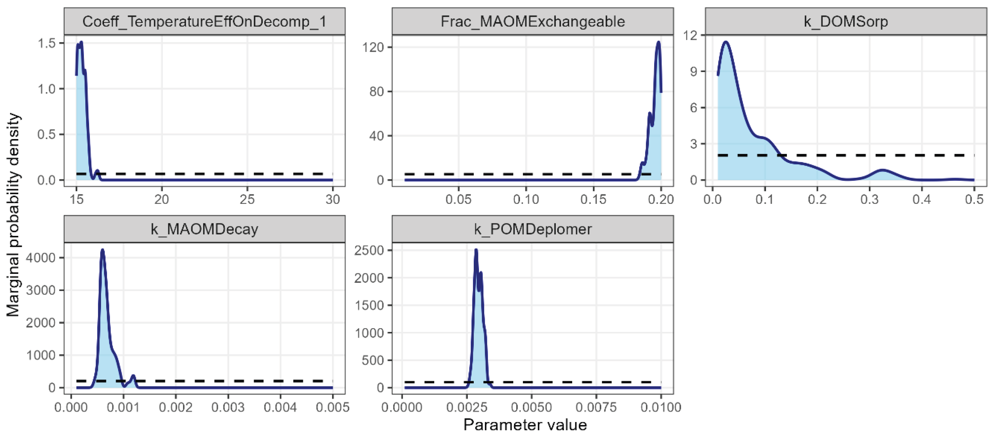
Figure 3.
Simulated and observed values of bulk soil organic carbon (SOC; A), particulate organic carbon (POC; B), mineral-associated organic carbon (MAOC; C), and annual cumulative net ecosystem exchange (NEE; D) across six NEON sites (CPER, DCFS, KONZ, NOGP, OAES, and WOOD) used for model calibration.
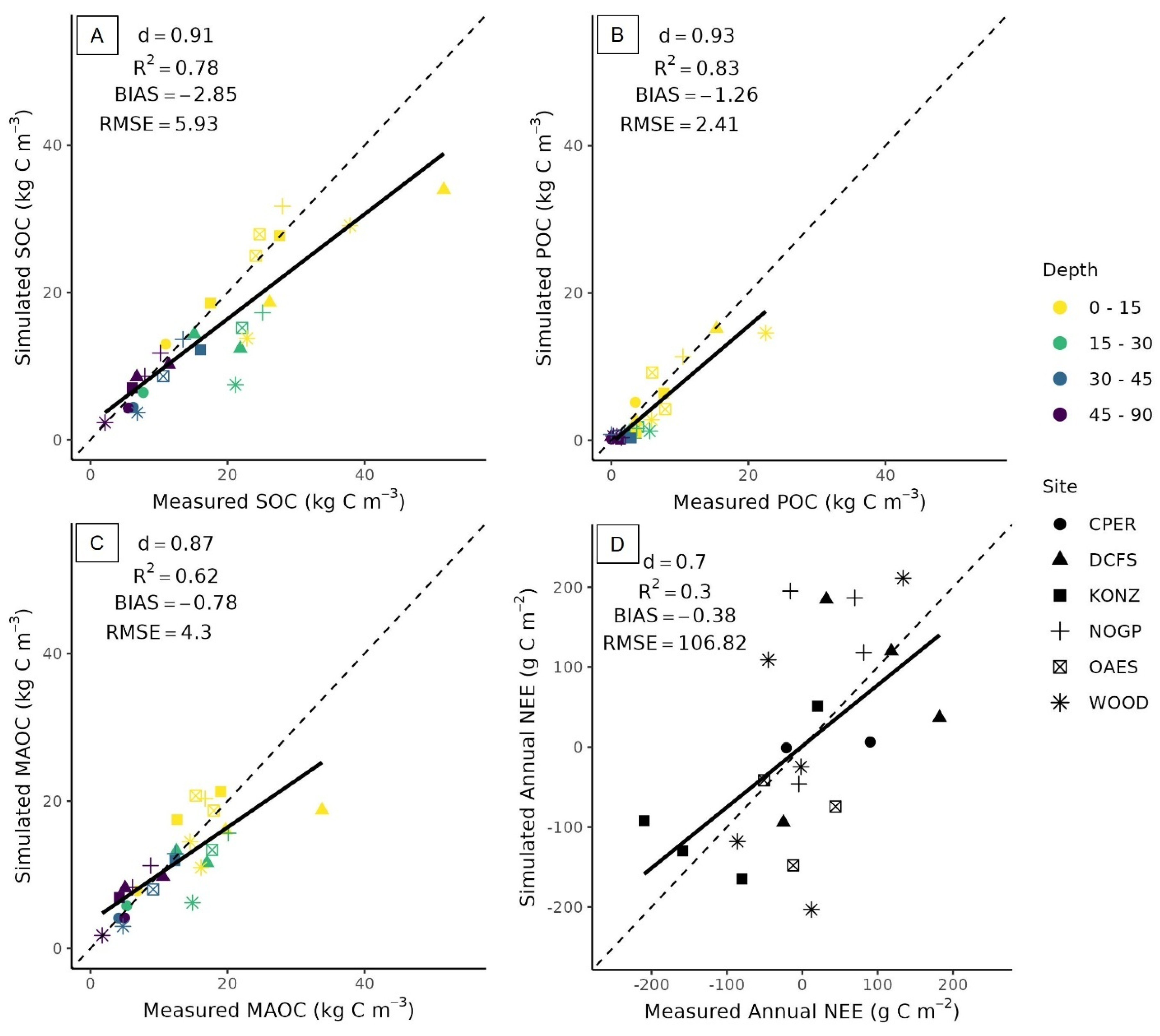
Figure 4.
Average observed and simulated values of bulk soil organic carbon (SOC; A), particulate organic carbon (POC; B), and mineral-associated organic carbon (MAOC; C) along the soil profile across experimental sites located in Oklahoma (OK-CR and OK-RR), Michigan (MI-LC), and Wyoming (WY-MR). Horizontal red bars represent the 2.5th-97.5th percentile ranges of observed values and horizontal teal bars represent the 95% posterior predictive intervals of simulated values. For simulated values, posterior predictive intervals were derived from the distribution of model outputs generated using the 200 parameter sets from the posterior of the Bayesian framework.
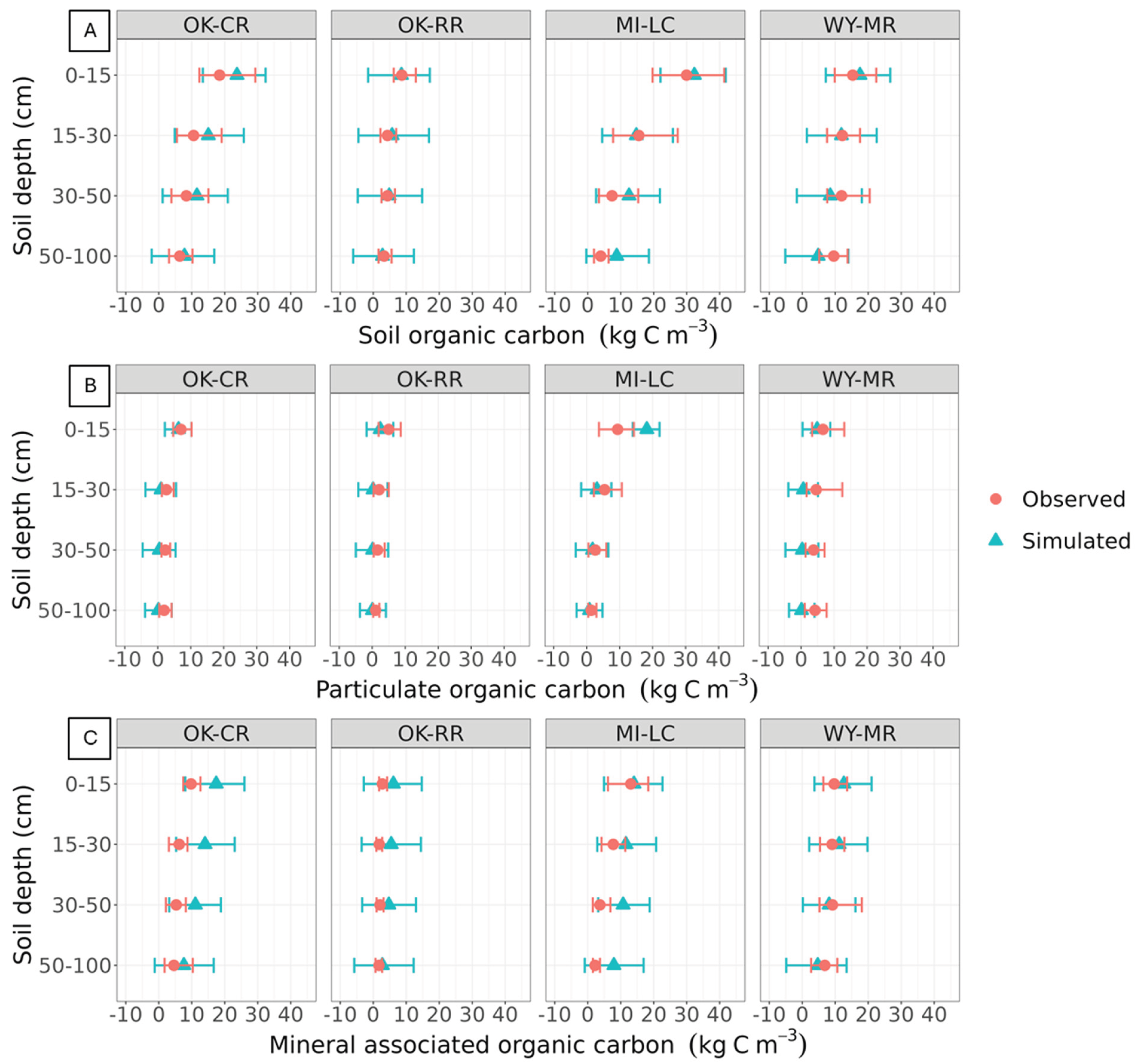
Figure 5.
Annual eddy covariance flux tower and simulated net ecosystem exchange (NEE) across blocks under adaptive (AD) and prescriptive (PR) grazing management for 2023 and 2024 at experimental sites located in Oklahoma (OK-CR: A-B; and OK- RR: C-D), Michigan (MI-LC: E-F), and Wyoming (WY-MR: G-H). Vertical bars represent 95% posterior predictive intervals of simulated values. For simulated values, posterior predictive intervals were derived from the distribution of model outputs generated using the 200 parameter sets from the posterior of the Bayesian framework.
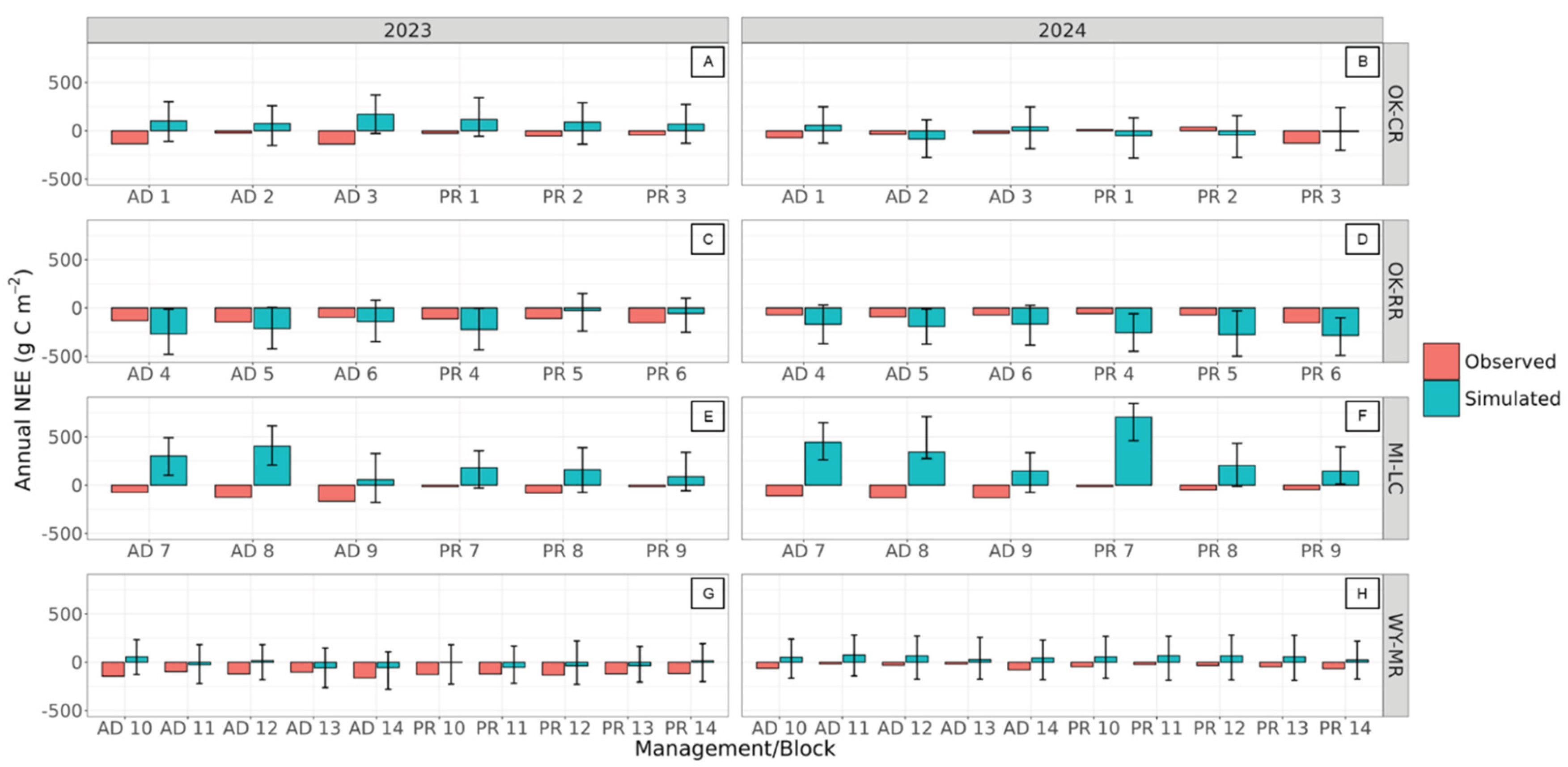

Table 1.
Site information for prescriptive (PR) and adaptive (AD) grazing management across experimental sites located in Oklahoma (OK-CR and OK-RR), Michigan (MI-LC), and Wyoming (WY-MR).
Table 1.
Site information for prescriptive (PR) and adaptive (AD) grazing management across experimental sites located in Oklahoma (OK-CR and OK-RR), Michigan (MI-LC), and Wyoming (WY-MR).
| Site name | Location | Altitude (m) | Koppen's climate classification | Dominant plant | # of blocks | Grazing management | Plot size (ha) | Paddock size (ha)* | Average plot resting period (day) | Length of grazing event (day) | Stocking rate (AU ha-1) |
| OK-CR | Oklahoma - Coffey Ranch | 250 | Humid subtropical (Cfa) | Warm-season grasses (e.g., Schizachyrium scoparium), but it also includes legumes and shrubs | 3 | PR | 11.5 | - | 104 | 1-13 | 1.9-6.3 |
| AD | 7.4 | 0.4-1.5 | 170 | 5-17 | 5-8.4 | ||||||
| OK-RR | Oklahoma - Red River Grazing Facility | 226 | Humid subtropical (Cfa) | Warm-season grasses, particularly bermudagrass (Cynodon dactylon), with some presence of annuals and forbs | 3 | PR | 9.7 | - | 76 | 2-11 | 4.3 |
| AD | 9.7 | 0.97-1.94 | 178 | 1 | 20.5-46.7 | ||||||
| MI-LC | Michigan - Lake City Research Center | 340 | Humid continental (Dfb) | Cool-season grasses (e.g., Dactylis glomerta, Poa pratensis, Bromus inermis) | 3 | PR | 4 | - | 81 | 2-16 | 7.8 |
| AD | 4 | 0.2-2 | 153 | 0.2-1 | 64-425 | ||||||
| WY-MR | Wyoming - McGuire Ranch | 2190 | Arid cold steppe (BSk) | Cool-season grasses (e.g., Pascopyrum smithii, Koeleria macrantha, Poa fendleriana) and sagebrush | 5 | PR | 38.8-148.5 | - | 308 | 70-77 | 0.3 |
| AD | 38.8-148.5 | - | 353 | 8-21 | 0.5-3.5 |
*PR grazing management plots were treated as one large paddock. AU: animal unit based on 500 kg (Allen et al., 2011).
Table 2.
Statistical metrics used to evaluate plant parameterization for NEON sites (CPER, DCFS, KONZ, NOGP, OAES, WOOD) using gross primary productivity (GPP) and for 3M project experimental sites (OK-CR, OK-RR, MI-LC, WY-MR) using aboveground biomass (ABG) and leaf area index (LAI).
Table 2.
Statistical metrics used to evaluate plant parameterization for NEON sites (CPER, DCFS, KONZ, NOGP, OAES, WOOD) using gross primary productivity (GPP) and for 3M project experimental sites (OK-CR, OK-RR, MI-LC, WY-MR) using aboveground biomass (ABG) and leaf area index (LAI).
| Dataset | Site name | Variable | Statistical metric | |||
| d | R2 | BIAS | RMSE | |||
| NEON | CPER | GPP (g C m-2 8-day sum) | 0.89 | 0.70 | -2.62 | 5.46 |
| DCFS | GPP (g C m-2 8-day sum) | 0.91 | 0.86 | -6.49 | 11.17 | |
| KONZ | GPP (g C m-2 8-day sum) | 0.95 | 0.86 | 2.18 | 9.94 | |
| NOGP | GPP (g C m-2 8-day sum) | 0.84 | 0.79 | -6.54 | 9.93 | |
| OAES | GPP (g C m-2 8-day sum) | 0.85 | 0.67 | 3.82 | 9.78 | |
| WOOD | GPP (g C m-2 8-day sum) | 0.95 | 0.82 | -1.82 | 9.03 | |
| 3M project | OK-CR | ABG (Mg ha-1) | 0.67 | 0.21 | 0.17 | 0.99 |
| LAI (m2 m-2) | 0.79 | 0.41 | -0.08 | 0.69 | ||
| OK-RR | ABG (Mg ha-1) | 0.64 | 0.13 | 0.07 | 0.71 | |
| LAI (m2 m-2) | 0.63 | 0.14 | 0.09 | 0.53 | ||
| MI-LC | ABG (Mg ha-1) | 0.59 | 0.29 | 0.88 | 1.61 | |
| LAI (m2 m-2) | 0.58 | 0.12 | -0.39 | 1.75 | ||
| WY-MR | ABG (Mg ha-1) | 0.50 | 0.05 | 0.04 | 0.15 | |
| LAI (m2 m-2) | - | - | - | - | ||
d: index of agreement; R2: coefficient of determination; RMSE: root mean square error.
Table 3.
Statistical metrics of data used for testing general model performance [soil temperature at 10 cm of depth, soil water content (SWC) at 15, 40 and 60 cm of depth], and model evaluation [weekly sum of net exchange ecosystem (NEE), gross primary productivity (GPP), and ecosystem respiration (ER)] across experimental sites located in Oklahoma (OK-CR and OK-RR), Michigan (MI-LC), and Wyoming (WY-MR).
| Location | Statistical metric | General model performance | Model evaluation | ||||||||
| Soil temperature10 cm | SWC15 cm | SWC40 cm | SWC60 cm | SOC | POC | MAOC | NEE | GPP | ER | ||
| ºC | cm3 cm-3 | kg C m-3 | g C m-2 week-1 | ||||||||
| OK-CR | d | 0.95 | 0.90 | 0.92 | 0.91 | 0.88 | 0.90 | 0.47 | 0.80 | 0.94 | 0.94 |
| R2 | 0.95 | 0.83 | 0.74 | 0.71 | 0.98 | 1.00 | 0.83 | 0.47 | 0.82 | 0.80 | |
| BIAS | -2.76 | 0.03 | 0.01 | -0.01 | 3.54 | -1.48 | 6.01 | 1.82 | -2.48 | -0.66 | |
| RMSE | 3.72 | 0.06 | 0.04 | 0.04 | 3.87 | 1.54 | 6.35 | 7.57 | 10.23 | 7.11 | |
| OK-RR | Soil temperature10 cm | SWC15 cm | SWC40 cm | SWC60 cm | SOC | POC | MAOC | NEE | GPP | ER | |
| d | 0.94 | 0.86 | 0.86 | 0.86 | 0.96 | 0.65 | 0.25 | 0.68 | 0.80 | 0.73 | |
| R2 | 0.93 | 0.78 | 0.79 | 0.74 | 0.88 | 0.97 | 0.50 | 0.25 | 0.52 | 0.65 | |
| BIAS | -3.84 | -0.04 | -0.03 | -0.01 | 0.33 | -1.71 | 2.66 | -1.60 | -5.76 | -7.36 | |
| RMSE | 4.53 | 0.05 | 0.05 | 0.05 | 0.79 | 1.80 | 2.85 | 7.71 | 11.80 | 9.67 | |
| MI-LC | Soil temperature10 cm | SWC15 cm | SWC40 cm | SWC60 cm | SOC | POC | MAOC | NEE | GPP | ER | |
| d | 0.95 | 0.76 | 0.83 | 0.87 | 0.96 | 0.80 | 0.68 | 0.79 | 0.86 | 0.84 | |
| R2 | 0.94 | 0.54 | 0.54 | 0.59 | 0.95 | 0.86 | 0.88 | 0.54 | 0.68 | 0.79 | |
| BIAS | -2.92 | 0.04 | 0.02 | -0.01 | 2.90 | 1.30 | 4.39 | 6.51 | 3.02 | 9.54 | |
| RMSE | 3.52 | 0.06 | 0.05 | 0.05 | 3.75 | 4.60 | 4.94 | 13.51 | 18.80 | 15.81 | |
| WY-MR | Soil temperature10 cm | SWC10 cm | SWC20 cm | SWC30 cm | SOC | POC | MAOC | NEE | GPP | ER | |
| d | 0.98 | 0.60 | 0.66 | 0.77 | 0.79 | 0.42 | 0.72 | 0.79 | 0.93 | 0.86 | |
| R2 | 0.94 | 0.26 | 0.38 | 0.48 | 0.95 | 0.95 | 0.81 | 0.59 | 0.78 | 0.70 | |
| BIAS | -1.57 | -0.05 | -0.05 | -0.02 | -1.53 | -3.29 | 0.51 | 1.91 | -0.45 | 1.46 | |
| RMSE | 2.83 | 0.07 | 0.06 | 0.04 | 3.14 | 3.41 | 2.20 | 3.82 | 3.70 | 3.08 | |
Disclaimer/Publisher’s Note: The statements, opinions and data contained in all publications are solely those of the individual author(s) and contributor(s) and not of MDPI and/or the editor(s). MDPI and/or the editor(s) disclaim responsibility for any injury to people or property resulting from any ideas, methods, instructions or products referred to in the content. |
© 2026 by the authors. Licensee MDPI, Basel, Switzerland. This article is an open access article distributed under the terms and conditions of the Creative Commons Attribution (CC BY) license.
Copyright: This open access article is published under a Creative Commons CC BY 4.0 license, which permit the free download, distribution, and reuse, provided that the author and preprint are cited in any reuse.


