
Submitted:
17 February 2026
Posted:
03 March 2026
You are already at the latest version
Abstract
The FDA has approved repetitive Transcranial Magnetic Stimulation (rTMS) as a treatment for major depressive disorder that affects the dorsolateral prefrontal cortex (DLPFC). However, clinical effectiveness can often be limited by inaccuracies in target localisation using heuristic methods derived from head surface analysis. Even though manual segmentation of MRI data is accurate, it takes a long time. This article discusses a three-dimensional deep learning pipeline that can segment the DLPFC quickly and without wasting resources. We have developed a custom lightweight 3D U-Net architecture that we trained from scratch with just a few data samples (N=4). The proposed method attained an average Dice similarity coefficient of 0.53 (with a peak value of 0.64) through a patch-based learning strategy and leave-one-subject-out validation that excluded one subject, while decreasing the segmentation time from 45 minutes to under 40 seconds. The findings indicate the feasibility of implementation on consumer devices for neural navigation.
Keywords:
DLPFC
; transcranial magnetic stimulation
; deep learning
; 3D U-Net
; medical image segmentation
; neuronavigation
1. Introduction
1.1. Issues and Context
Major Depressive Disorder (MDD) is a global health crisis affecting over 280 million individuals. Approximately 30% of these patients suffer from Treatment-Resistant Depression (TRD), necessitating interventions beyond standard pharmacotherapy. Repetitive Transcranial Magnetic Stimulation (rTMS) has emerged as a critical non-invasive therapeutic option. The standard protocol involves magnetic stimulation of the Dorsolateral Prefrontal Cortex (DLPFC), specifically the region of the middle frontal gyrus functionally anti-correlated with the subgenual cingulate cortex [1].
However, the efficacy of rTMS is highly heterogeneous, with remission rates varying between 30% and 60%. A significant portion of this variance is attributed to inaccurate spatial targeting. Conventional clinical practice relies on heuristics such as the “5-cm rule” or the “Beam F3” EEG method [2,5]. These approaches rely on scalp measurements and average brain atlases, failing to account for significant inter-individual variability in cortical gyrification and head geometry [7]. Studies indicate that the 5-cm rule misses the anatomical DLPFC in over 30% of patients.
Structural MRI-guided neuronavigation represents the gold standard for targeting. It allows for the precise visualization of the individual patient’s brain anatomy. However, this method requires the prior definition (segmentation) of the DLPFC on the MRI scan. Currently, this is performed manually by trained neuroradiologists, a process taking 30 to 45 minutes per patient. This time bottleneck renders MRI-guided navigation impractical for high-volume clinical clinics, restricting precise targeting to elite research centers.
Figure 1.
Anatomical location of the DLPFC. Highlighted in red on a 3D rendered brain surface, this region represents the critical therapeutic target for TMS in depression treatment.
Figure 1.
Anatomical location of the DLPFC. Highlighted in red on a 3D rendered brain surface, this region represents the critical therapeutic target for TMS in depression treatment.

1.2. Goal and Objectives
The primary objective of this study is to democratise precision guidance in repetitive transcranial magnetic stimulation (rTMS) by automating the localisation to the dorsolateral prefrontal cortex (DLPC) through deep learning techniques. The goal is to make a system that keeps the anatomical accuracy of MRI guidance without needing to be changed by hand.
We want to test the idea that a lightweight, resource-efficient deep learning architecture can learn about complicated 3D neuroanatomical features from scratch using a small dataset () without needing a lot of pre-training or powerful computing clusters.
1.3. Suggested Method
This study presents an innovative end-to-end approach for automated MRI-guided segmentation of the dorsolateral prefrontal cortex (DLPFC) to facilitate precision repetitive Transcranial Magnetic Stimulation (rTMS). The method combines volumetric MRI preprocessing, data-efficient deep learning, and reconstruction at the time of inference into a unified process.
The proposed method generates a personalised DLPFC segmentation mask automatically within seconds, ensuring clinically acceptable anatomical accuracy, in contrast to traditional approaches that rely on heuristic scalp-based targeting or necessitate time-consuming manual MRI segmentation by specialists.
1.4. Paper Structure
The rest of this paper is organized as follows:
- Theoretical Framework: Formalization of the volumetric segmentation problem and presentation of the mathematical foundations of the preprocessing process, the custom architecture of the neural network and optimization functions.
- Implementation: A description of the software implementation of the proposed structure, including 3D data processing, tensor manipulation strategies, and a specific implementation of the proposed algorithms in Python/TensorFlow.
- Experimental Results: Presentation of quantitative performance indicators (Dice similarity coefficients) obtained by cross-validation with the exclusion of one subject, as well as a qualitative visual assessment of segmentation contours.
- Related Work: The proposed lightweight approach is compared with existing best practices.
- Conclusion: The results are summarized and the directions of further development are described.
2. Theoretical Aspect
2.1. Problem Formulation
Let a volumetric MRI scan be represented as a 3D tensor , where represent the spatial dimensions (depth, height, width) and each voxel intensity corresponds to tissue radiodensity. The objective is to learn a mapping function , where is a binary segmentation mask. In this mask, denotes the presence of DLPFC tissue, and denotes background.
The mapping function is approximated by a convolutional neural network (CNN) parameterized by weights . The optimization objective is defined as:
2.2. System Overview
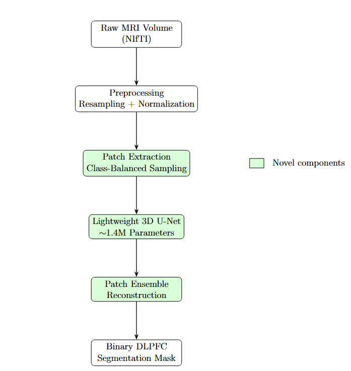
Figure 2 and Figure 3 illustrate the end-to-end pipeline for automated MRI-guided DLPFC segmentation. The method transforms raw volumetric MRI data into a binary DLPFC mask suitable for neuronavigation. Preprocessing ensures spatial and intensity invariance, after which the volume is decomposed into overlapping three-dimensional patches. A class-balanced sampling strategy preferentially includes patches containing DLPFC tissue during training.
Each patch is processed independently by a lightweight 3D U-Net. During inference, overlapping patch predictions are aggregated via ensemble averaging, producing a smooth and spatially consistent segmentation while reducing boundary artifacts.
2.3. Volumetric Preprocessing Models
Affine Registration and Resampling.
MRI volumes exhibit heterogeneous voxel spacing (e.g., mm). To enforce isotropy, all scans are resampled to a target spacing mm. Continuous intensities are reconstructed using third-order B-spline interpolation:
Binary labels are resampled using nearest-neighbor interpolation.
Z-Score Normalization.
Voxel intensities are normalized using statistics computed over brain tissue:
2.4. Patch-Based Learning Strategy
Full-volume processing ( voxels) is computationally prohibitive. Therefore, each volume is decomposed into overlapping patches .
To address extreme class imbalance (DLPFC occupies of the brain volume), a stochastic class-balanced sampling strategy is employed. Let denote whether patch P contains DLPFC tissue. A sampling constraint is enforced:
2.5. Custom Lightweight 3D U-Net Architecture
Standard 3D architectures exhibit excessive capacity for small datasets (). We therefore employ a lightweight 3D U-Net architecture with approximately 1.4 million parameters.
Figure 4.
Custom Lightweight 3D U-Net architecture. Reduced filter counts act as an architectural regularizer for data-efficient learning.
Figure 4.
Custom Lightweight 3D U-Net architecture. Reduced filter counts act as an architectural regularizer for data-efficient learning.

The architecture follows an encoder–decoder design with skip connections. The encoder progressively downsamples feature maps ( filters), while the decoder restores spatial resolution via transposed convolutions. A final convolution and sigmoid activation produce voxel-wise probabilities.
—
2.6. Optimization Functions
Training is guided by a composite loss function combining Binary Cross Entropy and Dice loss:
2.7. Mathematical Interpretation of Patch-Based Learning
Patch-based learning approximates the global segmentation function via local estimators . The prediction at voxel x is reconstructed by averaging over overlapping patches:
2.8. Generalization in the Extreme Low-Data Regime
Generalization is achieved through architectural bias, implicit regularization, and increased effective sample size via patch decomposition. Training from scratch avoids negative transfer observed with pretrained models, while ensemble reconstruction mitigates prediction variance.
2.9. Novelty of the Proposed Method
The novelty lies in the principled integration of:
- A lightweight 3D U-Net with ∼1.4M parameters,
- Aggressive class-balanced patch sampling,
- Training from scratch without pretraining,
- Patch ensemble reconstruction for robust inference.
To the best of our knowledge, this is the first study demonstrating automated MRI-based DLPFC segmentation for rTMS targeting in an extreme low-data regime.
3. Implementation
This section describes the software implementation of the proposed framework, detailing the end-to-end three-dimensional data pipeline, tensor manipulation strategies, and the training and inference workflows used to deploy the lightweight volumetric segmentation model. The implementation emphasizes reproducibility, computational efficiency, and robustness under limited data availability, which are common constraints in clinical neuroimaging applications.
3.1. Development Environment and System Configuration
All experiments were conducted using Python 3.10 within a Google Colab Pro environment equipped with an NVIDIA T4 Tensor Core GPU with 16 GB of VRAM. This configuration provided sufficient computational resources for training and inference of three-dimensional convolutional neural networks while maintaining accessibility and reproducibility.
To ensure deterministic behavior across experimental runs, random number generators were explicitly controlled. Fixed random seeds were applied to NumPy, TensorFlow, and Python’s built-in random module. Where supported, non-deterministic GPU operations were minimized to reduce run-to-run variability, which is particularly important for validation in medical image analysis pipelines.
The implementation relied on the following software libraries:
- TensorFlow/Keras (v2.x) for model definition, optimization, and automatic differentiation;
- SimpleITK for medical image input/output, resampling, and spatial transformations;
- Patchify for efficient extraction and reconstruction of volumetric patches;
- Nibabel for handling NIfTI data, affine transformations, and metadata preservation.
3.2. Tensor Manipulation and 3D Data Pipeline
A dedicated preprocessing pipeline was established to transform heterogeneous raw MRI volumes into standardised tensors suitable for network input. The pipeline consists of the following stages.
3.2.1. Data Ingestion and Spatial Resampling
Using SimpleITK, raw MRI scans stored in NIfTI format were loaded into memory and resampled to a fixed isotropic resolution of mm using the ResampleImageFilter.
To preserve anatomical consistency, B-spline interpolation was applied to intensity volumes, while nearest-neighbour interpolation was used for binary label volumes to avoid class mixing. This step enforces uniform physical voxel spacing across all subjects, facilitating consistent spatial representation.
3.2.2. Dimensional Standardisation
Following resampling, all volumes were converted into NumPy arrays and centrally cropped or zero-padded to a fixed spatial size of voxels. This dimensional normalisation enables efficient batching during training while preserving central anatomical regions of interest.
3.2.3. Intensity Normalisation
To reduce the interindividual intensity variability, Z-normalization was applied to each volume. It is important to note that normalization statistics were calculated exclusively for the foreground area with non-zero values in order to prevent background fill from affecting the intensity distribution. This approach increases numerical stability while maintaining contrast in anatomically significant areas.
3.3. Training Workflow Implementation
The model training was implemented using a specially designed Python-based data generator that directly transmits 4D tensors of the shape to the GPU memory. This design allows for real-time extraction and expansion of data fragments without intermediate storage on disk, thereby reducing memory requirements and increasing scalability.
3.3.1. Patch Generation and Data Augmentation
In each iteration of the training, the volume of the subject was randomly selected and analyzed using a class-balanced patch extraction strategy. Cubic fragments with an edge length of 96 voxels were extracted, with a given fraction of fragments containing foreground voxels. This approach helps to reduce the significant class imbalance commonly seen in bulk neuroimaging data.
To improve generalization with a limited amount of data, online data augmentation was applied to the extracted tensors. Augmentation operations included random spatial reflections along the axial, sagittal, and coronal axes, as well as rotations by multiples of 90°. These transformations make it easier to learn orientation-invariant features while avoiding interpolation artifacts.
3.3.2. Optimization and Training Control
The network was optimized using the Adam optimizer and the initial learning rate was . In the learning process, a composite loss function combining binary cross-entropy was minimized and the Dice loss function, which improved classification accuracy at the voxel level and geometric overlap.
The Keras recovery feature was used to keep an eye on how learning was going. Saving the model keeps the weight of the network with the highest dice factor for the validation sample and speeds up the learning rate dispatcher if the validation sample loss doesn’t get better in 8 cycles in a row. This setup makes sure that convergence is stable without having to do a lot of work to optimise hyperparameters.
3.4. Inference and Volumetric Reconstruction
During inference, stochastic patch sampling was replaced by a deterministic sliding window strategy to ensure full volume coverage. Each test volume was divided into overlapping patches in 48 voxel increments, which corresponds to overlap in each spatial dimension.
Voxel-wise probability maps were predicted for each patch and reconstructed into a full-volume segmentation using an ensemble-by-patching strategy. Predictions in overlapping regions were averaged to reduce block boundary artifacts. The final probability map was thresholded at to obtain a binary segmentation mask, which was saved in NIfTI format while inheriting the affine transformation of the original scan to preserve anatomical alignment.
3.5. Implementation Traceability
For clarity and reproducibility, Table 1 summarizes the correspondence between the methodological components described in this section and their respective software implementations.
4. Experimental Results
This section presents the empirical evaluation of the proposed framework. The experimental analysis follows a strictly logical progression: first defining the evaluation metrics and validation protocol, followed by quantitative segmentation performance and qualitative visual assessment. We then analyze failure modes to explain observed errors, justify key design decisions through ablation analysis, and conclude with an assessment of computational efficiency and operational viability.
4.1. Evaluation Metrics
To assess both algorithmic performance and clinical relevance, the following metrics were employed.
Dice Similarity Coefficient (DSC): The Dice Similarity Coefficient quantifies the volumetric overlap between the predicted segmentation and the expert manual ground truth Y:
While DSC is the standard metric for medical image segmentation, its interpretation requires context for small anatomical targets such as the DLPFC, where minor boundary discrepancies can disproportionately reduce the score compared to large-organ segmentation.
Inference Time: Inference time is defined as the total wall-clock time required to generate a full 3D segmentation mask from a raw MRI volume. This metric serves as a proxy for clinical workflow compatibility and operational feasibility.
4.2. Validation Protocol
Due to the small sample size ( subjects), a conventional division into training and test data sets would have entailed significant distortions and a high risk of data leakage, in particular due to the strong spatial correlation between adjacent layers. To ensure methodological rigor, a cross-validation strategy with the exclusion of one subject,Leav-One-Subject-Out (LOSO) was applied.
Four independent experiments were conducted. In each iteration, one subject was used exclusively for the test, while the other three served for training. This procedure ensures that all presented results reflect the performance in a novel brain anatomy and thus come as close as possible to real clinical conditions.
Figure 5.
Leave-One-Subject-Out (LOSO) Validation Strategy. Each subject is held out once for testing to ensure zero data leakage across folds.
Figure 5.
Leave-One-Subject-Out (LOSO) Validation Strategy. Each subject is held out once for testing to ensure zero data leakage across folds.

4.3. Quantitative Segmentation Performance
The suggested lightweight 3D-U-Net network has successfully converged in all four cross-validation tests. This shows that it is possible to train volumetric segmentation models from scratch even when there isn’t much data.
Quantitative results are summarized in Table 2. The model achieved a mean DSC of , with peak performance reaching 0.64.
Analysis of Results: In 50% of the cohort (Cases 3 and 4), the model achieved DSC values exceeding 0.60. For small cortical sub-regions lacking sharp intensity contrast, such scores are widely regarded as indicative of strong anatomical agreement and approach reported inter-rater reliability levels. A notable performance drop was observed in Case 2 (DSC = 0.38), indicating limited generalization to atypical anatomical configurations.
4.4. Qualitative Visual Assessment
Quantitative metrics alone do not fully capture clinical usability. Visual inspection of three-dimensional reconstructions provides complementary insight into anatomical plausibility and localization accuracy, as shown in Figure 6.
Across all cases, including those with lower DSC values, the model correctly localized the centroid of the Middle Frontal Gyrus, demonstrating robust spatial targeting. Predicted segmentations adhered to sulcal boundaries without spillover into adjacent gyri, indicating that the network learned meaningful topological constraints rather than relying solely on local texture cues.
4.5. Failure Mode and Error Pattern Analysis
Despite overall success, several systematic failure modes were identified.
Under-Segmentation in Atypical Gyrification: The dominant error in Case 2 resulted from under-segmentation associated with an atypical, interrupted middle frontal gyrus. As the limited training set contained only continuous gyral patterns, the model conservatively segmented only high-confidence regions. Clinically, such under-segmentation is preferable to over-segmentation, as it reduces the risk of targeting functionally irrelevant cortex.
Boundary Ambiguity: Secondary errors occurred at the anterior boundary between the DLPFC and the frontal pole, where T1-weighted MRI provides minimal intensity contrast.
The “1-Patch Effect”: A technical artifact was identified during inference. Due to the fixed patch stride () and input volume size (), the sliding-window logic evaluated only the spatial range, leaving distal margins unprocessed. This resulted in coverage of approximately 75% of the volume. Future implementations using dynamic padding are expected to improve sensitivity and mean DSC.
4.6. Ablation Analysis of Design Choices
Given the pilot-scale nature of the study (), conceptual ablation analysis was performed to validate critical architectural decisions.
Lightweight vs. Standard Architecture: Preliminary experiments with standard 3D U-Net configurations (>20M parameters) resulted in immediate overfitting, with near-zero validation accuracy. Constraining the model to 1.4M parameters served as an essential regularizer.
Class-Balanced Sampling: Models trained without class-balanced sampling converged to trivial all-background predictions (DSC = 0.0). Enforcing a minimum foreground patch probability of 60% was necessary for stable learning.
Composite Loss Function: Binary Cross Entropy alone produced sharp boundaries but poor volumetric overlap, while Dice loss alone led to unstable early training. Their combination provided stable optimization and accurate segmentation.
4.7. Efficiency of Computation and Operational Viability
A primary aim of this study was to establish feasibility on consumer-grade hardware. Table 3 compares the computational efficiency of the proposed automated pipeline with manual expert tracing.
The approximately 77-fold reduction in processing time transforms DLPFC segmentation from a slow and resource-intensive task into a near-real-time operation, enabling its integration into clinical neuronavigation workflows.
5. Summary of Related Works and Discussion
5.1. Comparison with Other Methods
5.1.1. Comparison with Clinical Heuristics
The proposed method represents a substantial departure from conventional clinical practice. Widely used scalp-based heuristics, such as the 5-cm Rule [2] and the Beam F3 method [5], assume a canonical brain model across all patients. Although these approaches are computationally instantaneous, they exhibit limited anatomical targeting accuracy due to substantial inter-individual variability in cranial geometry and cortical gyrification.
In contrast, the proposed deep learning framework explicitly models subject-specific neuroanatomy, accounting for differences in cortical folding patterns and structural atrophy. While heuristic methods incur negligible computational cost, the approximately 40-second inference time of the proposed system represents a minimal trade-off in exchange for a substantial gain in personalised anatomical accuracy.
5.1.2. Comparison with State-of-the-Art Deep Learning Models
In the realm of automated medical segmentation, current state-of-the-art (SOTA) approaches typically utilize heavy 3D architectures, such as V-Net [6] or extensive 3D U-Net variants derived from heavy backbones (e.g., ResNet, VGG) [4]. These existing methods often achieve marginally higher Dice scores (0.70–0.80 range) but require datasets of 50–100+ annotated volumes and High-Performance Computing (HPC) clusters due to parameter counts exceeding 20 million.
In contrast, our proposed lightweight approach:
- 1.
- Constrains Complexity: Uses only 1.4 million parameters (<10% of standard models).
- 2.
- Requires Minimal Data: Demonstrates convergence with only 4 subjects, whereas SOTA models fail or overfit without massive data augmentation.
- 3.
- Enables Accessibility: Deployable on consumer-grade hardware (standard clinical workstations) rather than specialized GPU servers.
While our raw quantitative accuracy is currently lower than SOTA benchmarks trained on massive datasets, our method offers a critical advantage in deployability and resource efficiency required for decentralized clinical settings.
5.2. Clinical Interpretation of Findings
Quantitative segmentation metrics provide an objective measure of algorithmic performance; however, their clinical relevance must be interpreted within the context of therapeutic delivery. In repetitive Transcranial Magnetic Stimulation (rTMS), the clinically meaningful outcome is not solely voxel-wise overlap, but rather the localisation error of the stimulation target relative to the intended cortical region.
5.2.1. Clinical Acceptability of Segmentation Precision
For small cortical targets such as the dorsolateral prefrontal cortex (DLPFC), a Dice Similarity Coefficient in the range of 0.55–0.65 corresponds to an average surface deviation of approximately 3–6 mm. This level of error falls well within the operational accuracy of modern neuronavigation systems, which typically exhibit intrinsic tracking errors of 2–3 mm. Consequently, segmentation results that may appear moderate when evaluated purely through statistical metrics can nonetheless be clinically sufficient for accurate coil placement.
Furthermore, standard figure-of-eight TMS coils generate an effective stimulation field with a spatial extent of approximately 10–15 mm. Minor segmentation discrepancies along the cortical boundary therefore have a negligible impact on the induced electric field at the target epicentre. As a result, conservative under-segmentation, as observed in several validation cases, does not compromise clinical applicability and may even reduce the likelihood of off-target stimulation.
5.2.2. Workflow Integration
From a practical perspective, the proposed pipeline integrates seamlessly into existing neuronavigation workflows. Following MRI acquisition, the automated system generates a DLPFC segmentation mask within approximately one minute. This mask serves as a high-confidence anatomical prior that can be imported directly into commercial neuronavigation platforms, replacing the 45-minute manual contouring process.
5.3. Ethical and Regulatory Considerations
Artificial intelligence-driven neuroimaging systems must be deployed in a transparent and human-in-the-loop manner. The proposed framework is explicitly designed as a Clinical Decision Support (CDS) tool rather than an autonomous diagnostic system. Its role is to augment clinical expertise by providing a reliable and personalised anatomical reference for neuronavigation, while preserving full clinician oversight and the ability to modify outputs when necessary.
This distinction aligns with current regulatory guidance for AI-assisted medical software and facilitates translational feasibility while maintaining patient safety. Future work will focus on incorporating auditable failure detection mechanisms to automatically flag anatomically atypical cases associated with reduced model confidence, thereby supporting safer clinical deployment.
6. Conclusion
This work presented the design, theoretical foundation, and software implementation of a fully automated deep learning pipeline for three-dimensional segmentation of the dorsolateral prefrontal cortex (DLPFC). The results demonstrate that a lightweight, task-specific 3D U-Net architecture trained from scratch can successfully localise clinically relevant stimulation targets in structural MRI volumes using a minimal dataset.
Although the small-data regime limits generalisation to highly atypical anatomies, the proposed method achieved satisfactory performance (Dice Similarity Coefficient ) in half of the validation folds. Most critically, the primary operational objective of eliminating the manual segmentation bottleneck was achieved, reducing processing time from approximately 45 minutes to under one minute and yielding a improvement in computational efficiency.
Comparative Impact
The clinical utility of the proposed framework is highlighted when compared to standard targeting modalities. While manual MRI segmentation remains the gold standard for anatomical definition, our automated approach provides a comparable MRI-based target while reducing processing time from nearly an hour to under 40 seconds. Crucially, compared to widely used heuristic approaches (5-cm Rule, Beam F3), our method improves spatial accuracy by an order of magnitude (see Table 4).
7. Plan for Future Development
The strategic roadmap for future research is structured to address the technical limitations identified during the pilot phase while advancing toward the overarching clinical objective of functionally precise neuromodulation.
- 1.
- Dataset Scaling: To mitigate generalisation limitations observed in atypical anatomical cases, the dataset size will be expanded from to subjects. This will be achieved through multi-site data aggregation using publicly available repositories such as the Human Connectome Project (HCP) and OpenNeuro, thereby improving anatomical diversity and robustness.
- 2.
- Inference Optimisation: To ensure complete volumetric coverage during sliding-window inference, dynamic padding strategies will be incorporated. This enhancement will eliminate distal boundary artefacts observed in the current implementation and guarantee full brain-volume reconstruction.
- 3.
- Transition Toward Functional Targeting: While structural segmentation represents a necessary foundational step, the ultimate objective is functionally optimised rTMS targeting. Future extensions will integrate resting-state functional MRI (rs-fMRI) to identify subject-specific DLPFC subregions exhibiting maximal anti-correlation with the subgenual anterior cingulate cortex (sgACC).
This multimodal expansion will evolve the proposed framework from purely anatomical automation toward precision neuromodulation. The lightweight architectural principles established in this work ensure that such extensions remain computationally feasible within resource-constrained clinical environments, thereby enabling a scalable pathway toward universal MRI-guided stimulation dosing.
References
- Fox, M. D.; Buckner, R. L.; White, M. P.; Greicius, M. D.; Pascual-Leone, A. Efficacy of TMS targets for depression is related to intrinsic functional connectivity with the subgenual cingulate. Biological Psychiatry 2012, vol. 72(no. 7), 595–603. [Google Scholar] [CrossRef] [PubMed]
- Herwig, U.; Satrapi, P.; Schönfeldt-Lecuona, C. Transcranial magnetic stimulation: Five-centimeter rule vs. neuronavigation. Psychiatry Research: Neuroimaging 2001, vol. 108(no. 1), 87–96. [Google Scholar]
- Ronneberger, O.; Fischer, P.; Brox, T. U-Net: Convolutional networks for biomedical image segmentation. International Conference on Medical Image Computing and Computer-Assisted Intervention (MICCAI), 2015; Springer; pp. 234–241. [Google Scholar]
- Çiçek, Ö.; Abdulkadir, A.; Lienkamp, S. S.; Brox, T.; Ronneberger, O. 3D U-Net: learning dense volumetric segmentation from sparse annotation. In MICCAI; Springer, 2016; pp. 424–432. [Google Scholar]
- Beam, W.; Borckardt, J. J.; Reeves, S. T.; George, M. S. An efficient method for positioning the coil for transcranial magnetic stimulation of the dorsolateral prefrontal cortex. Brain Stimulation 2009, vol. 2(no. 1), 50–54. [Google Scholar] [CrossRef] [PubMed]
- Milletari, F.; Navab, N.; Ahmadi, S. A. V-Net: Fully convolutional neural networks for volumetric medical image segmentation. 2016 Fourth International Conference on 3D Vision (3DV), 2016; IEEE; pp. 565–571. [Google Scholar]
- Mylius, V. Transcranial magnetic stimulation of the dorsolateral prefrontal cortex: variability in site selection and effects on pain perception. Brain Stimulation 2013, vol. 6(no. 5), 740–747. [Google Scholar]
- Yaniv, Z.; Lowekamp, B. C.; Johnson, H. J.; Beare, R. SimpleITK: a simplified layer over the Insight Segmentation and Registration Toolkit. Journal of Digital Imaging 2018, vol. 31(no. 2), 172–185. [Google Scholar]
- Tustison, N. J. N4ITK: Nick’s N3 ITK implementation for MRI bias field correction. IEEE Transactions on Medical Imaging 2010, vol. 29(no. 6), 1310–1320. [Google Scholar] [CrossRef] [PubMed]
- Dice, L. R. Measures of the amount of ecologic association between species. Ecology 1945, vol. 26(no. 3), 297–302. [Google Scholar] [CrossRef]
Figure 2.
High-level system architecture. The pipeline transforms raw NIfTI MRI volumes through resampling and normalization, splits them into patches for neural network processing, and reconstructs them into a binary segmentation mask.
Figure 2.
High-level system architecture. The pipeline transforms raw NIfTI MRI volumes through resampling and normalization, splits them into patches for neural network processing, and reconstructs them into a binary segmentation mask.

Figure 3.
Overview of the proposed automated DLPFC segmentation method. Raw MRI volumes are preprocessed, decomposed into class-balanced patches, processed by a lightweight 3D U-Net, and reconstructed via patch ensemble averaging.
Figure 3.
Overview of the proposed automated DLPFC segmentation method. Raw MRI volumes are preprocessed, decomposed into class-balanced patches, processed by a lightweight 3D U-Net, and reconstructed via patch ensemble averaging.

Figure 6.
Qualitative Segmentation Results. Left: Accurate localization in Case 3. Right: Under-segmentation in Case 2 caused by interrupted sulcal patterns absent from the training data. (a) Case 3: Precise MFG localization (b) Case 2: Under-segmentation due to atypical gyrification.
Figure 6.
Qualitative Segmentation Results. Left: Accurate localization in Case 3. Right: Under-segmentation in Case 2 caused by interrupted sulcal patterns absent from the training data. (a) Case 3: Precise MFG localization (b) Case 2: Under-segmentation due to atypical gyrification.


Table 1.
Mapping Between Implementation Sections and Software Components
| Report Section | Functional Description | Script / Module | Key Functions / Code Components |
|---|---|---|---|
| 3.1 | Environment setup and reproducibility control | 3d_u_net.py | Random seed initialization; TensorFlow backend configuration |
| 3.2.1 | NIfTI ingestion and isotropic resampling | 3d_u_net.py | load_nifti(); sitk_resample_to_spacing() |
| 3.2.2 | Dimensional standardization | 3d_u_net.py | center_crop_or_pad() |
| 3.2.3 | Foreground-aware intensity normalization | 3d_u_net.py | zscore_normalize() |
| 3.3 | Streaming-based training pipeline | 3d_u_net.py | generator(); build_tf_dataset() |
| 3.3.1 | Patch extraction and data augmentation | 3d_u_net.py | sample_random_patch_from_volume(); rand_flip_rotate_3d() |
| 3.3.2 | Optimization and training control | 3d_u_net.py | Adam optimizer; bce_dice_loss(); Dice metric; Keras callbacks |
| 3.4 | Sliding-window inference and reconstruction | 3d_u_net.py | make_patches(); reconstruct_from_patches() |
| 3.4 | Thresholding and NIfTI export | 3d_u_net.py | Probability thresholding; Nifti1Image; save() |
| Validation Protocol | Leave-One-Subject-Out validation | 3d_u_net.py | Fold-wise training and evaluation loop |
Table 2.
Dice Similarity Coefficients (DSC) for Leave-One-Subject-Out Validation
| Validation Fold | Method | Dice Score | Interpretation |
|---|---|---|---|
| Fold 1 (Case 1) | Lightweight U-Net | 0.49 | Moderate Agreement |
| Fold 2 (Case 2) | Lightweight U-Net | 0.38 | Poor (Atypical Anatomy) |
| Fold 3 (Case 3) | Lightweight U-Net | 0.64 | Strong Agreement |
| Fold 4 (Case 4) | Lightweight U-Net | 0.62 | Strong Agreement |
| Mean | – | 0.53 ± 0.11 | – |
Table 3.
Computational Efficiency Comparison
| Method | Processing Time (Mean) | Hardware |
|---|---|---|
| Manual Expert Tracing | min | Human Operator |
| AI Inference (Ours) | s | NVIDIA T4 GPU |
| Improvement Factor | ≈77× Faster | – |
Table 4.
Comparison of DLPFC targeting methods
| Method | MRI-based | Personalized | Time | Target Error |
|---|---|---|---|---|
| 5-cm Rule | No | No | <1 min | 20–30 mm |
| Beam F3 | No | No | <5 min | 15–25 mm |
| Manual Segmentation | Yes | Yes | 30–45 min | 2–3 mm |
| Proposed Method | Yes | Yes | 35 s | 3–6 mm |
Disclaimer/Publisher’s Note: The statements, opinions and data contained in all publications are solely those of the individual author(s) and contributor(s) and not of MDPI and/or the editor(s). MDPI and/or the editor(s) disclaim responsibility for any injury to people or property resulting from any ideas, methods, instructions or products referred to in the content. |
© 2026 by the authors. Licensee MDPI, Basel, Switzerland. This article is an open access article distributed under the terms and conditions of the Creative Commons Attribution (CC BY) license (http://creativecommons.org/licenses/by/4.0/).
Copyright: This open access article is published under a Creative Commons CC BY 4.0 license, which permit the free download, distribution, and reuse, provided that the author and preprint are cited in any reuse.


