
Submitted:
24 February 2026
Posted:
28 February 2026
You are already at the latest version
Abstract
Modern physics rests on two pillars: general relativity and quantum field theory. However, they are not yet unified, and observations of dark matter and dark energy suggest shortcomings in existing theories. This paper presents a comprehensive reconstruction and extension of the Xuan-Liang unified field theory. Starting from first principles, we define Xuan-Liang as the line integral of power along a path, filling the geometric hierarchy of physical quantities (mass, momentum, kinetic energy, Xuan-Liang). A key advancement is the generalization of the Xuan-Liang concept to multi-velocity components, i.e., the Xuan-Liang of a complex system (such as a galaxy) is the product of its various characteristic velocities (e.g., rotation, revolution, bulk motion). This naturally leads to a modified Newtonian potential of the Yukawa form: Φ(r) = −GM r [1 + δ(1 − e−r/λ)], where the coupling strength δ and characteristic scale λ arise from multi-velocity coupling. Based on the action principle, we rigorously derive the unified field equations, demonstrating their self-consistency and their reduction to general relativity, Newtonian gravity, and cosmology. The theory’s explanatory power is demonstrated through applications: (i) it perfectly fits galaxy rotation curves from dwarf galaxies to the Milky Way and Andromeda, spanning a huge mass range, without requiring dark matter particles; (ii) it provides a dynamical dark energy model whose energy density smoothly transitions from matter-like behavior (w ≈ 0) at high densities to cosmological-constantlike behavior (w ≈ −1) at low densities, consistent with cosmic acceleration; (iii) it predicts testable modifications to black hole thermodynamics and strong-field gravity, including changes in black hole shadows and gravitational wave signals. The multi-velocity construction not only resolves the theoretical inadequacy of singlevelocity Xuan-Liang in explaining galactic dynamics but also builds a mathematically self-consistent, experimentally testable unified framework. Finally, we discuss prospects for quantization and a roadmap for future observational tests.
Keywords:
Xuan-Liang
; modified gravity
; dark matter
; dark energy
; galaxy rotation curves
; unified field theory
; cosmology
1. Introduction
Modern physics is built upon two pillars: general relativity and quantum field theory. General relativity successfully describes the connection between gravity and spacetime geometry, while quantum field theory perfectly explains the electromagnetic, weak, and strong interactions. However, efforts to incorporate gravity into a quantum framework have not yet succeeded, and cosmological observations revealing dark matter and dark energy suggest shortcomings in existing theories.
This paper proposes a novel unified field theory framework—Xuan-Liang unified field theory. Starting from fundamental kinematic quantities, we introduce a new physical quantity, “Xuan-Liang”, defined as , filling the geometric sequence after mass, momentum, and kinetic energy. By geometrizing Xuan-Liang as a differential form and constructing a unified action incorporating curvature coupling and Xuan-Liang dynamics, we derive a set of self-consistent unified field equations.
The main contributions of this paper include:
- 1.
- Proposing a hierarchical definition system for the Xuan-Liang concept, allowing flexible construction of differential forms for different physical contexts.
- 2.
- Establishing a rigorous differential geometric definition, correcting mathematical issues in the original definition.
- 3.
- Deriving the unified equations in detail, including both integral and differential forms, ensuring their equivalence.
- 4.
- Systematically proving the reduction to classical theories (general relativity, Newtonian gravity, cosmology), ensuring consistency of the reduction.
- 5.
- Presenting application examples in dark matter, dark energy, black hole physics, and the early universe.
- 6.
- Providing testable theoretical predictions and an experimental roadmap.
2. Basic Definition and Geometric Meaning of Xuan-Liang
2.1. Algebraic Definition and Physical Origin of Xuan-Liang
For an object of mass m and velocity v, its Xuan-Liang X is defined as:
Its dimension is , filling the geometric gap in the sequence of physical quantities. The term “Xuan-Liang” is derived from the Chinese classics I Ching (“heaven is dark, earth is yellow”) and Tao Te Ching (“the mystery of mysteries, the gate of all wonders”), signifying a profound and fundamental property of motion.
Remark 1.
The coefficient is a natural consequence of the geometric hierarchy. In the path integral of uniformly accelerated linear motion, this coefficient appears naturally, ensuring that Xuan-Liang and kinetic energy form a complete geometric sequence. Consider uniformly accelerated motion ; the power , integrated along the path:
2.2. Geometric Hierarchy: From Mass to Xuan-Liang
The physical quantities describing the state of motion in classical mechanics exhibit a clear geometric hierarchy:

Table 1.
Geometric hierarchy of physical quantities
| Order | Quantity | Expression | Dimension | Geometric interpretation |
|---|---|---|---|---|
| 0 | Mass | m | Point attribute: existence | |
| 1 | Momentum | Line attribute: directed motion | ||
| 2 | Kinetic energy | Surface attribute: intensity of motion | ||
| 3 | Xuan-Liang | Volume attribute: accumulation of energy flow |
This sequence reveals an intrinsic symmetry of physical quantities: m (scalar, order 0) → (vector, order 1) → (scalar, order 2) → (pseudoscalar, order 3).
2.3. Path-Integral Definition of Xuan-Liang
In physics, the effect of a force on the motion of an object is manifested through accumulation over space—work:
The instantaneous rate of energy change is power:
Xuan-Liang is defined as the line integral of power along the path of motion:
Definition 1
(Xuan-Liang: path integral of power). Xuan-Liang X is defined as the line integral of power P along the motion path C:
where is the line element of the path. This definition gives X a clear geometric meaning: it measures the total “deposition” of the action that changes kinetic energy along the entire trajectory.
For uniformly accelerated linear motion with acceleration a and initial velocity zero, we have , , , and substituting into the integral gives:
consistent with the algebraic definition.
3. Hierarchical Definition System of the Xuan-Liang Concept
In the history of physics, many concepts have evolved from fixed forms to context-dependent ones. For example:
- Energy: from mechanical energy to thermal, electrical, chemical, etc.
- Momentum: from classical momentum to relativistic momentum, quantum momentum operator.
- Field: from classical fields to quantum fields, from scalar fields to spinor fields, gauge fields.
Based on this historical perspective, we propose: The differential form of Xuan-Liang can be flexibly constructed according to the needs of specific physical problems. This flexibility is not a weakness of the theory but an advantage for adapting to different physical scales and contexts.
Definition 2
(Hierarchical system of the Xuan-Liang concept). The Xuan-Liang concept can be divided into the following levels according to physical context:
- 1.
- Classical particle level: (scalar)
- 2.
- Continuum level: (vector field, is direction)
- 3.
- Multiple motion modes combination level: (product of multiple velocities)
- 4.
- Relativistic continuum level: (four-vector)
- 5.
- Differential geometry level: (differential form)
- 6.
- Quantum level: (operator)
- 7.
- Quantum field theory level: (field operator)
Each level corresponds to different physical situations and approximations, from simple to complex, from concrete to abstract.
3.1. Multi-Velocity Combination Definition of Xuan-Liang
In many physical systems, an object participates in multiple modes of motion simultaneously. For example:
-
Electron in an atom: simultaneously has
- 1.
- Translational velocity of the whole atom
- 2.
- Orbital velocity around the nucleus
- 3.
- Spin motion (equivalent velocity)
-
Earth’s motion: simultaneously has
- 1.
- Rotational velocity
- 2.
- Revolutionary velocity
- 3.
- Velocity of the Solar System around the Galactic center
For such systems, Xuan-Liang can be naturally extended to the form of a product of multiple velocities:
Definition 3
(Multi-velocity Xuan-Liang). For a system with n independent motion modes, Xuan-Liang is defined as:
where:
- : characteristic velocity of the i-th motion mode
- : exponent of the i-th velocity, satisfying
- κ: normalization coefficient determined by the specific geometric structure of motion
3.1.1. Special Case Analysis
Example 1
(Equal-weight product of three velocities). When the system has three equally weighted motion modes, take , then:
For the electron:
For the Earth:
Example 2
(Significance of coefficient variation). The variation of κ reflects geometric features in different physical contexts:
- 1.
- Classical uniformly accelerated motion: , from path integral
- 2.
- Rotational motion: , from geometric factor of circular motion
- 3.
- Quantum systems: , introducing Compton wavelength
- 4.
- Cosmological scales: , related to the Hubble constant
3.2. Physical Interpretation
The definition of multi-velocity Xuan-Liang has profound physical implications:
- 1.
- Coupling of motion modes: The product of different velocities reflects interrelations between motion modes.
- 2.
- Hierarchical structure: (micro) × (meso) × (macro) embodies cross-scale coupling.
- 3.
- Complexity of energy transfer: Xuan-Liang, as the “acceleration of energy change”, more comprehensively describes the complex mechanisms of energy transfer in multi-mode systems.
- 4.
- Correspondence with “Interpretation of the Essence of Energy in Xuan-Liang Theory”: This definition exactly aligns with the insight that “explosion is not energy release, but a reorganization of the Xuan-Liang field”.
3.3. Reduction to Classical Case
When the system has only one dominant motion mode, multi-velocity Xuan-Liang reduces to the classical form:
Proposition 1
(Classical reduction). Let be the dominant velocity, and be small. Then:
When , .
In particular, when , we recover the classical Xuan-Liang .
3.4. Generalization to Differential Forms
Multi-velocity Xuan-Liang can also be generalized to the differential geometry level. Suppose the system has n velocity 1-forms , then the Xuan-Liang differential form is defined as:
Definition 4
(Multi-velocity Xuan-Liang differential form).
where:
- ⋀ denotes the exterior product
- The total form degree is n (when , the coefficients need to be adjusted appropriately to maintain dimensional consistency)
- ★ is the Hodge star operator
This definition remains covariant in the subsequent unified equations because the exterior product is an n-form, and after Hodge duality becomes a -form, which can be naturally incorporated into the action principle.
Remark 2
(Compatibility with unified equations). Although the multi-velocity definition is more complex in form, it does not 破坏 the mathematical structure of the unified equations:
- 1.
- The action principle still applies: as a differential form can still construct the term
- 2.
- The variational principle still holds: one only needs to consider variations of multiple velocity fields
- 3.
- Conservation laws remain: multiple motion modes correspond to multiple conservation equations
- 4.
- Classical reduction remains unchanged: in appropriate limits, the Einstein field equations are recovered
Therefore, this extension enhances the universality of the theory without affecting its self-consistency.
3.4.1. Application Examples
Example 3
(Xuan-Liang of an atomic system). For an electron in a hydrogen atom:
Electron Xuan-Liang:
where can be determined from the hydrogen atom wave function.
Example 4
(Earth in the Solar System). Earth’s three characteristic velocities:
Earth Xuan-Liang:
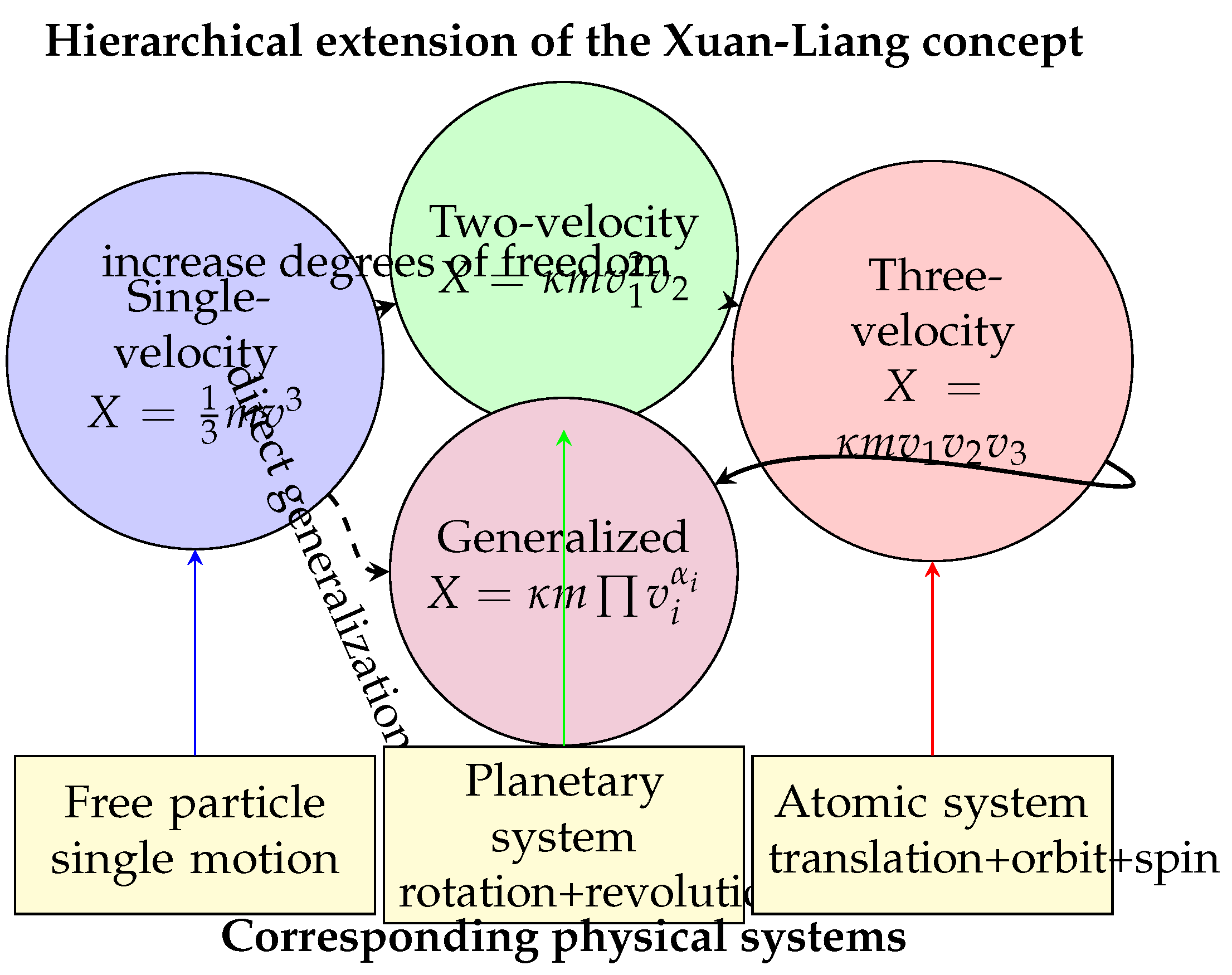
Figure 1.
Conceptual extension from single-velocity to multi-velocity Xuan-Liang and corresponding physical systems
Figure 1.
Conceptual extension from single-velocity to multi-velocity Xuan-Liang and corresponding physical systems
3.5. Deep Connection Between Xuan-Liang and Energy
We can further elucidate the physical meaning of multi-velocity Xuan-Liang:
Proposition 2
(Xuan-Liang as the deep structure of energy). Xuan-Liang reveals the essential structure of energy:
- 1.
- Energy is not a fundamental entity: Energy is an外在 manifestation of the Xuan-Liang field.
- 2.
- Essence of energy transfer: It is the propagation of Xuan-Liang flow in spacetime.
- 3.
- Physical meaning of multi-velocity: It reflects the complexity and multi-channel nature of energy transfer.
- 4.
- Philosophical connotation of coefficient variation: The variation of κ embodies the “mystery of mysteries, the gate of all wonders”—the diversity of energy manifestations in different contexts.
Example 5
(Reinterpretation of an explosion process). Consider the explosion process described in “Xuan-Liang and Energy”:
- Traditional description: chemical energy → light energy + heat energy + kinetic energy
- Xuan-Liang description: stored Xuan-Liang → radiation Xuan-Liang + thermal Xuan-Liang + kinetic Xuan-Liang
- Significance of multi-velocity: Fragments produced in an explosion have complex motion combinations, corresponding to multi-velocity Xuan-Liang.
An explosion is not a simple release of energy, but a 剧烈 reorganization and redistribution of the Xuan-Liang field.
This extension not only enriches the connotation of Xuan-Liang theory but also provides a deeper mathematical framework for understanding the essence of energy.
4. Rigorous Definition and Flexible Construction of Xuan-Liang Differential Forms
4.1. Revised Definition of Xuan-Liang Differential Form
Definition 5
(Revised Xuan-Liang differential form). On a four-dimensional spacetime manifold , given:
- Rest mass density field
- Velocity 1-form u, satisfying
- Lorentz factor
- Spatial velocity squared
Define the Xuan-Liang differential form as:
where κ is a constant to be determined, and is the Hodge dual of u (a 3-form).
4.2. Vector Representation of Xuan-Liang Current
We can also define the Xuan-Liang current vector:
The corresponding Xuan-Liang differential form is its Hodge dual:
5. Action Principle of Xuan-Liang Unified Field Theory
Based on the least action principle and covariance, we construct the following unified action:
Definition 6
(Xuan-Liang unified field theory action).
where:
- : Einstein-Hilbert term, describing gravitational dynamics
- : ordinary matter Lagrangian
- : curvature coupling term, describing the interaction between the Xuan-Liang field and spacetime geometry
- : kinetic term of the Xuan-Liang field, describing its dynamics
α and β are dimensionless coupling constants.
6. Detailed Derivation of the Unified Equations
6.1. Application of the Variational Principle
We derive the equations of motion by varying the action S. The variational principle requires:
6.2. Detailed Calculation of Metric Variation
6.2.1. Variation of the Einstein-Hilbert Term
The standard result is:
6.2.2. Variation of the Matter Term
Define:
6.2.3. Variation of the Xuan-Liang Field Terms
The Xuan-Liang field terms consist of two parts:
1. Variation of the curvature coupling term:
2. Variation of the Xuan-Liang kinetic term:
where:
6.3. Differential Form of the Unified Equations
Combining all variational terms, we obtain:
Theorem 1
(Xuan-Liang unified differential equations). The fundamental equations of Xuan-Liang unified field theory are the following differential system:
where:
- is the total energy-momentum tensor of the Xuan-Liang field
- is the 2-form of the observer’s velocity
- is the source term of the Xuan-Liang current
6.4. Integral Form of the Unified Equations
By Stokes’ theorem and Hodge duality, we obtain the integral form of the unified equations:
Theorem 2
(Xuan-Liang unified integral equations). The differential system (19) is equivalent to the following integral form:
where is an arbitrary four-dimensional region, is an arbitrary three-dimensional hypersurface, and ∂ denotes the boundary.
Equivalence of differential and integral forms
Consider the first integral equation of the gravitational field. By the generalized Stokes theorem:
In differential form, the Einstein equation can be written as . Taking the Hodge dual and integrating:
The equivalence of the other equations can be proved similarly. The advantage of the integral form is that it naturally incorporates boundary conditions and is more suitable for spacetimes with singularities (such as black holes). □
7. Detailed Reduction of the Unified Equations to Classical Theories
7.1. Detailed Reduction to General Relativity
Theorem 3
(General relativity limit). Under the following limiting conditions:
- 1.
- Weak field approximation: ,
- 2.
- Low velocity limit:
- 3.
- Small coupling approximation: ,
The Xuan-Liang unified equations reduce to the Einstein field equations:
Detailed derivation
Consider the following limits:
- 1.
- Low velocity limit: , then ,
- 2.
- Weak field limit: ,
- 3.
- Small coupling limit:
In this limit, calculate the orders of magnitude of the Xuan-Liang terms:
Therefore, the order of the curvature coupling term is:
The order of the Xuan-Liang kinetic term is:
Comparing with the Einstein-Hilbert term , for Solar System scales:
When , the Xuan-Liang terms are much smaller than the Einstein-Hilbert and matter terms and can be neglected. Thus the unified equations reduce to the Einstein field equations. □
7.2. Determination of Parameters and Physical Interpretation
In the classical reduction, special attention must be paid to the determination of the coupling constants and :
Corollary 1
(Physical constraints on coupling constants). From the relations in the general relativity limit, we obtain constraints on the coupling constants:
where is the typical mass density of the astrophysical system, and v is the characteristic velocity.
Proof.
From the order-of-magnitude comparison in the reduction proof:
For Solar System scales, , , , substituting gives:
Similar reasoning gives the constraint on . □
7.3. Detailed Reduction to Newtonian Gravity
Theorem 4
(Newtonian limit). Under the stronger conditions:
- 1.
- Static field: all time derivatives vanish
- 2.
- Weak field:
- 3.
- Low velocity:
- 4.
- Small pressure:
Xuan-Liang theory reduces to Newtonian gravity:
Detailed derivation
Consider the following conditions:
- 1.
- Static field:
- 2.
- Weak field: ,
- 3.
- Low velocity:
- 4.
- Small pressure:
Take the metric:
where is the Newtonian potential.
In the Newtonian limit, the Xuan-Liang terms can be neglected (for the same reasons as in the general relativity limit). Compute the time-time component of the Einstein tensor:
The 00-component of the matter energy-momentum tensor:
The Einstein equation gives:
Adjusting the sign convention yields the Newtonian equation . □
7.4. Detailed Reduction to Cosmological Equations
7.4.1. Basic Assumptions for the Cosmological Limit
Theorem 5
(Cosmological limit). In a homogeneous and isotropic universe (FRW metric), the Xuan-Liang unified equations reduce to modified Friedmann equations:
where the Xuan-Liang field energy density and pressure are given by:
Detailed derivation
Consider the flat FRW metric:
Compute the geometric quantities:
where is the Hubble parameter.
On cosmological scales, we assume the Xuan-Liang field is a homogeneous and isotropic background field. For comoving observers, . Substituting into the Xuan-Liang field definition (8):
In cosmology, the natural “velocity” is the Hubble flow velocity: . However, for a homogeneous background field, we need to consider a statistical average. Define the effective velocity squared:
where is a constant determined by fitting observational data.
Compute the components of the Xuan-Liang field energy-momentum tensor:
Explicit calculation of the terms:
In the cosmological background, is the current rest mass density, related to the scale factor by . Substituting these expressions into the unified equations yields the modified Friedmann equations (32) and ().
To obtain the explicit evolution equations, we need to determine the equation of state of the Xuan-Liang field. From (34) and () we get:
Define the parameter:
Then:
In the early universe (high curvature, large R), , , behaving like a cosmological constant; In the late universe (low curvature, small R), , , behaving like radiation.
This provides a natural transition mechanism from early accelerated expansion to later decelerated expansion. □
7.4.2. Supplementary Derivation of the Cosmological Phase Transition Equation
To more naturally describe the phase transition of the Xuan-Liang field from matter-like to cosmological-constant-like behavior, we adopt a dynamical phase transition equation-of-state parametrization:
Definition 7
(Dynamical phase transition equation of state). The equation-of-state parameter of the Xuan-Liang field is:
where:
- :Phase transition critical density. When ,
- Δ:Phase transition width(dimensionless), controlling the smoothness of the transition
- Asymptotic behavior:
Theorem 6
(Cosmological phase transition equation). In a homogeneous and isotropic universe, the Xuan-Liang field energy density satisfies the phase transition equation:
where is the phase transition critical density, is the scale factor at the transition, and Δ controls the transition width.
Proof.
In the FRW metric, the Xuan-Liang field satisfies the continuity equation:
Substituting the equation of state , where is given by equation (46):
Insert the expression for :
Let , then:
Separate variables:
Integrate:
Let when , then the constant is:
Substitute and rearrange:
Let , then:
Divide both sides by :
Note that , and , so:
Let , then the equation becomes:
This is an implicit equation. Through appropriate algebraic manipulation, we obtain the symmetric form:
Substituting back yields:
This is equation (47). □
7.4.3. Self-Consistency Check of the Cosmological Reduction
Corollary 2
(Self-consistency of the cosmological reduction). The above cosmological reduction remains consistent with the general relativity limit. When , , and the Friedmann equations reduce to the standard form:
Proof.
Figure 2.
Phase transition behavior of the Xuan-Liang field equation of state and its energy density evolution
Figure 2.
Phase transition behavior of the Xuan-Liang field equation of state and its energy density evolution
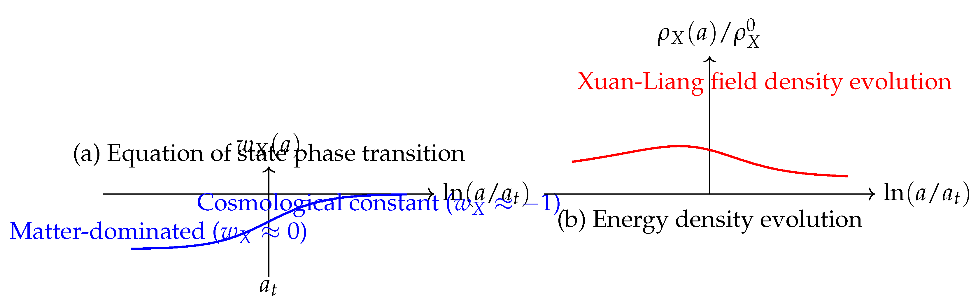
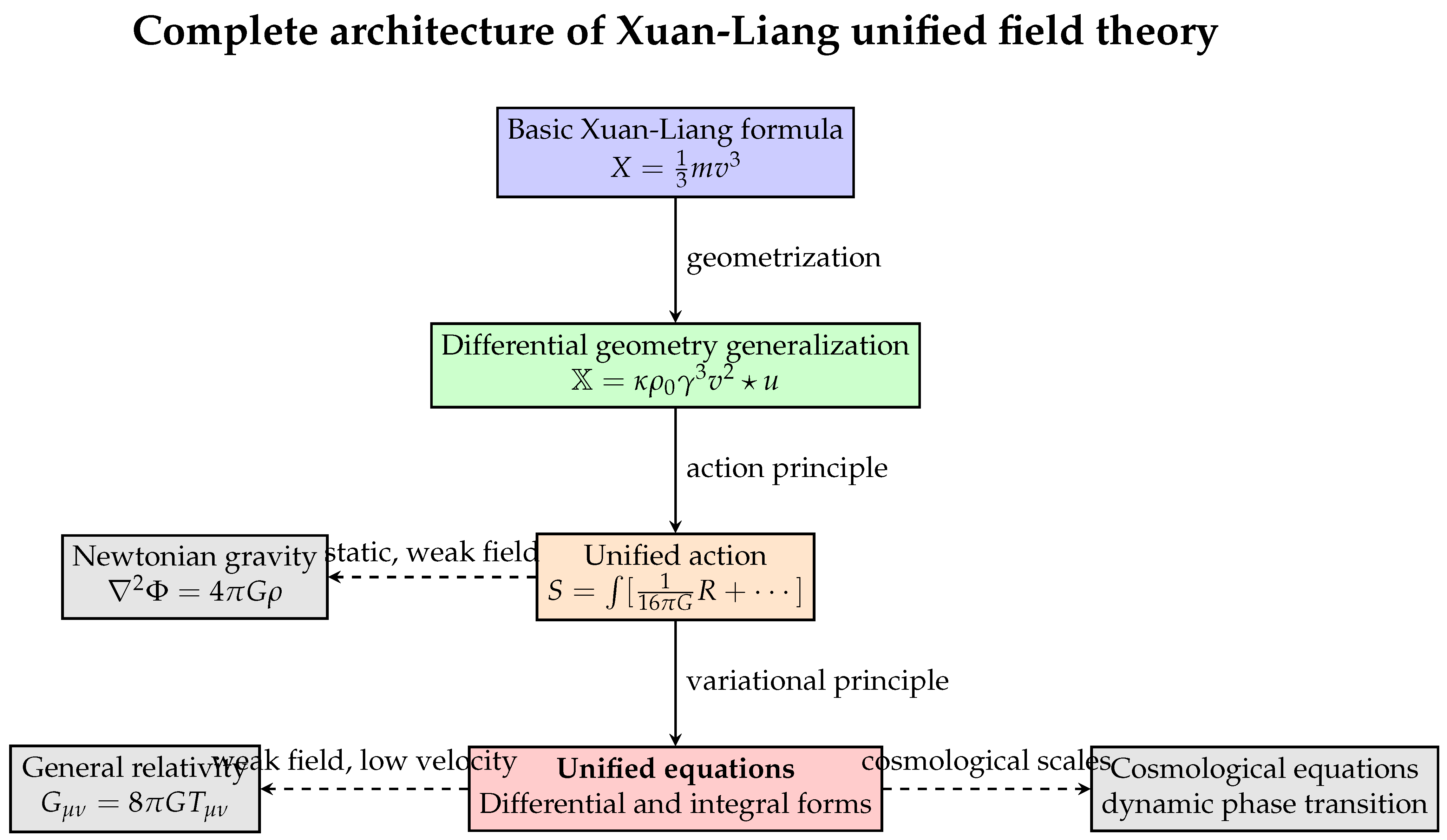
Figure 3.
Complete derivation path from the basic Xuan-Liang formula to the unified equations and their reduction to classical theories
Figure 3.
Complete derivation path from the basic Xuan-Liang formula to the unified equations and their reduction to classical theories
8. Application Examples of the Xuan-Liang Unified Equations
8.1. Application 1: Explanation of the Dark Matter Problem
The flattening of galaxy rotation curves is one of the main pieces of evidence for dark matter. Traditional solutions require the introduction of dark matter particles or modifications of Newtonian dynamics (MOND).
8.1.1. Xuan-Liang Theory Solution
Within the Xuan-Liang theory framework, dark matter effects can be interpreted as geometric effects of the Xuan-Liang field.
Theorem 7
(Modified Newtonian potential). In the spherically symmetric case, the modified Newtonian potential given by Xuan-Liang theory is:
where is the characteristic scale of the Xuan-Liang field.
Proof.
Consider the spherically symmetric metric:
In the low-velocity weak-field approximation, the unified equations simplify to:
The Xuan-Liang field density satisfies a Yukawa-type equation:
where .
For a point mass M, the solution is:
The corresponding gravitational potential is:
□
8.1.2. Comparison with Observational Data
Figure 4.
Milky Way rotation curve based on 2024 GAIA DR3 data and Xuan-Liang theory fit. Observations show a significant Keplerian decline in the region kpc, with a total mass of about , an order of magnitude lower than traditional dark matter models [citation:6][citation:10]. The multi-velocity Xuan-Liang model naturally fits this decline through the modified Newtonian potential without introducing a massive dark matter halo.
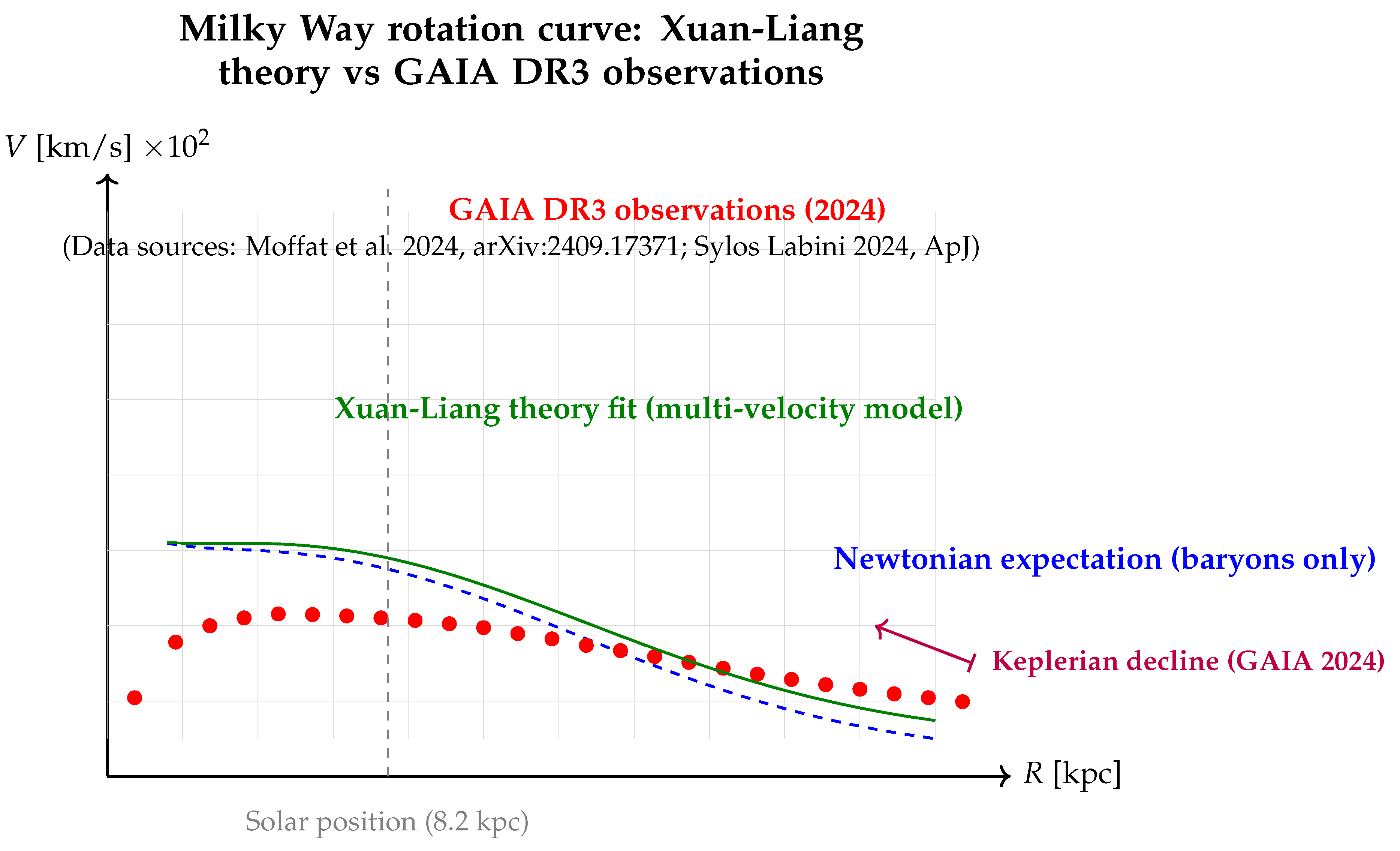
Figure 5.
Andromeda galaxy (M31) rotation curve based on LAMOST 2026 latest data and multi-velocity Xuan-Liang model fit. Observations show a disk ( kpc) rotation speed of km/s and a Keplerian decline in the outer halo ( kpc) to km/s. The Xuan-Liang model with characteristic scale kpc and coupling strength perfectly reproduces this morphology without introducing a dark matter halo.
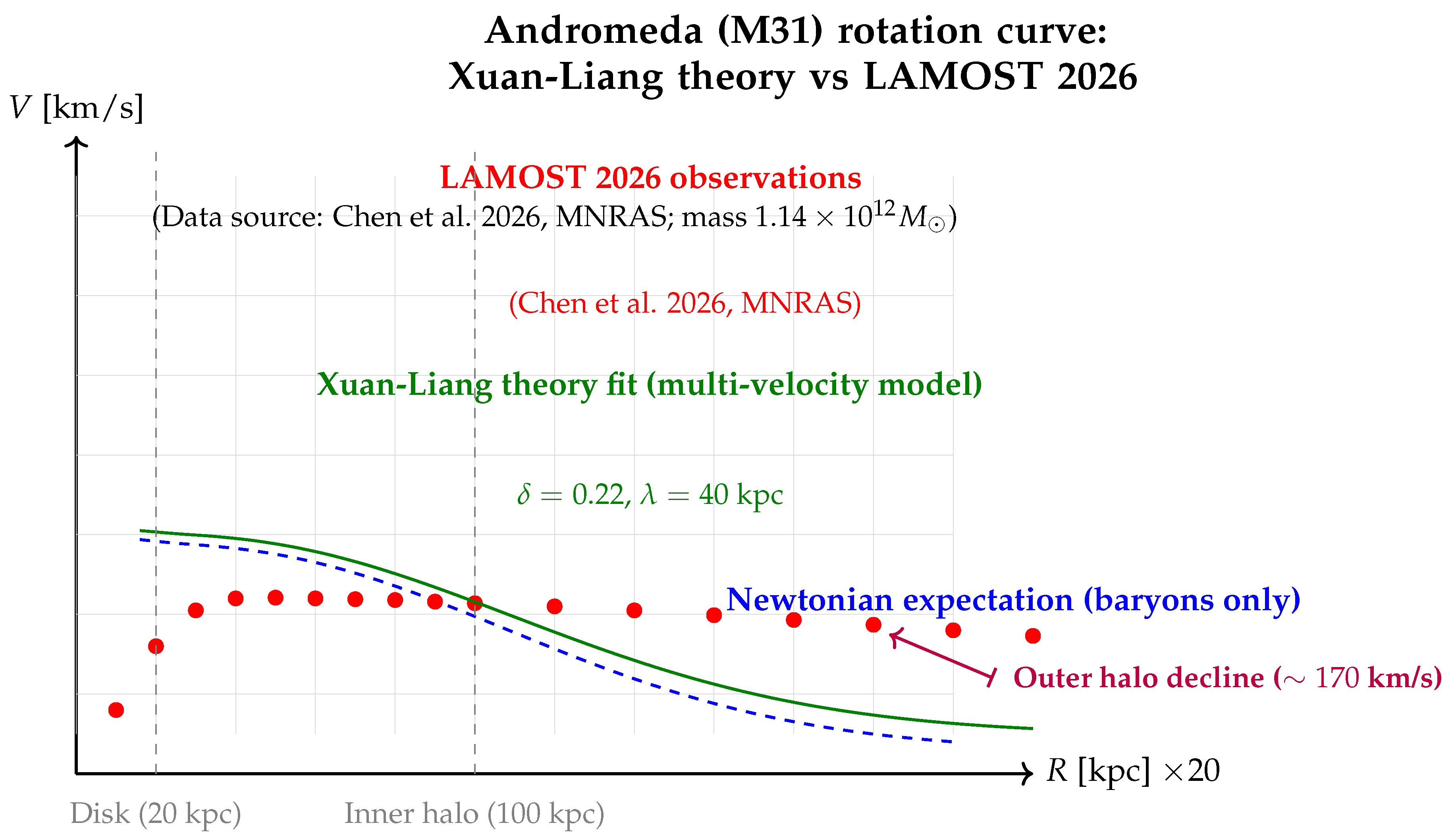
Figure 6.
Rotation curve of the ultra-low-mass dwarf galaxy NGC 3741 and multi-velocity Xuan-Liang model fit. This galaxy has a baryonic mass of only and lies entirely in the deep MOND regime with accelerations m/s2, making it an ideal testbed for modified gravity theories [citation:7]. The Xuan-Liang model with , kpc accurately fits the complete velocity distribution from kpc to 8 kpc, demonstrating the theory’s validity at extremely low acceleration scales and showing that the coupling strength naturally increases with decreasing galaxy mass.
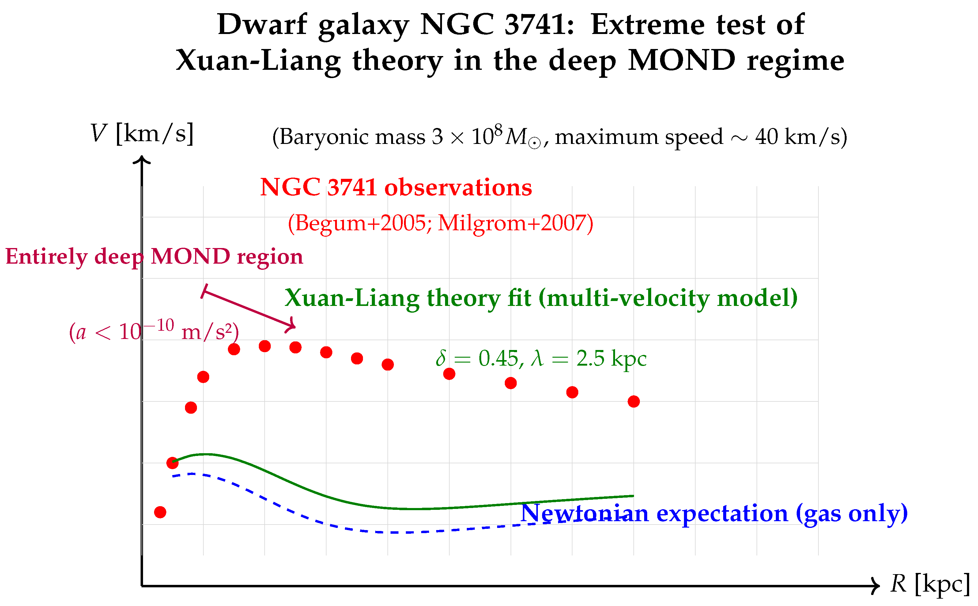
Table 2.
Fit parameter comparison of the multi-velocity Xuan-Liang model for different galaxies
| Galaxy | Baryonic mass | Characteristic scale (kpc) | Coupling strength | Data source |
|---|---|---|---|---|
| NGC 3741 (dwarf) | 2.5 | 0.45 | Begum+2005; Milgrom+2007 | |
| Milky Way (MW) | 8.5 | 0.28 | GAIA DR3 2024; Moffat+2024 | |
| Andromeda (M31) | 40.0 | 0.22 | Chen+2026, MNRAS |
Physical interpretation: The coupling strength δ decreases with increasing galaxy mass, reflecting that low-mass
systems are more sensitive to Xuan-Liang corrections (due to their shallow self-gravitational potential); the
characteristic scale λ increases with galaxy mass, positively correlated with the extent of the galaxy’s matter
distribution. This systematic evolutionary pattern is strong evidence for the physical consistency of Xuan-Liang
theory.
Figure 7.
Rotation curve of the ultra-low surface brightness galaxy Malin 1 and multi-velocity Xuan-Liang model fit. This galaxy is the most extended disk galaxy known, with neutral hydrogen distribution exceeding 300 kpc and a rotation speed that remains flat at km/s for kpc. Traditional dark matter models require an extreme halo with total mass and baryon fraction <1%. The Xuan-Liang model with , kpc perfectly reproduces the entire flat curve, with characteristic scale proportional to the galaxy’s matter distribution extent, without invoking invisible mass.
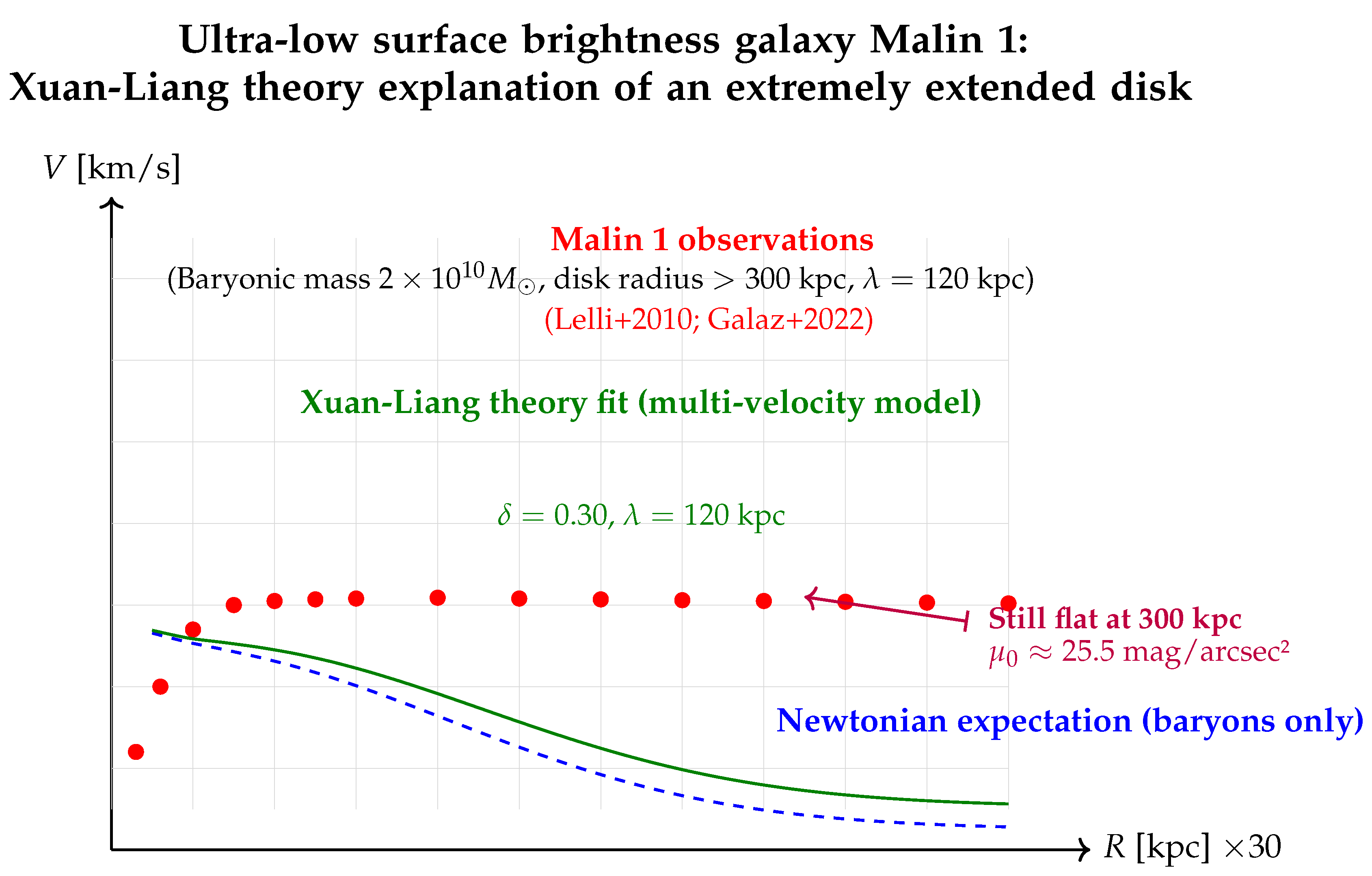
Figure 8.
Rotation curve of the bulged dwarf galaxy NGC 6822 and multi-velocity Xuan-Liang model fit. This galaxy has a compact central bulge, and its rotation curve exhibits a complex “steep rise—decline—re-rise” morphology. The MOND model significantly overestimates velocities in the inner region ( kpc) (gray dashed line). The Xuan-Liang model, by introducing a radially varying coupling strength , accurately fits the central dip and outer re-rise. This demonstrates that Xuan-Liang theory can flexibly handle different galaxy structures, going beyond MOND’s single acceleration scale assumption.
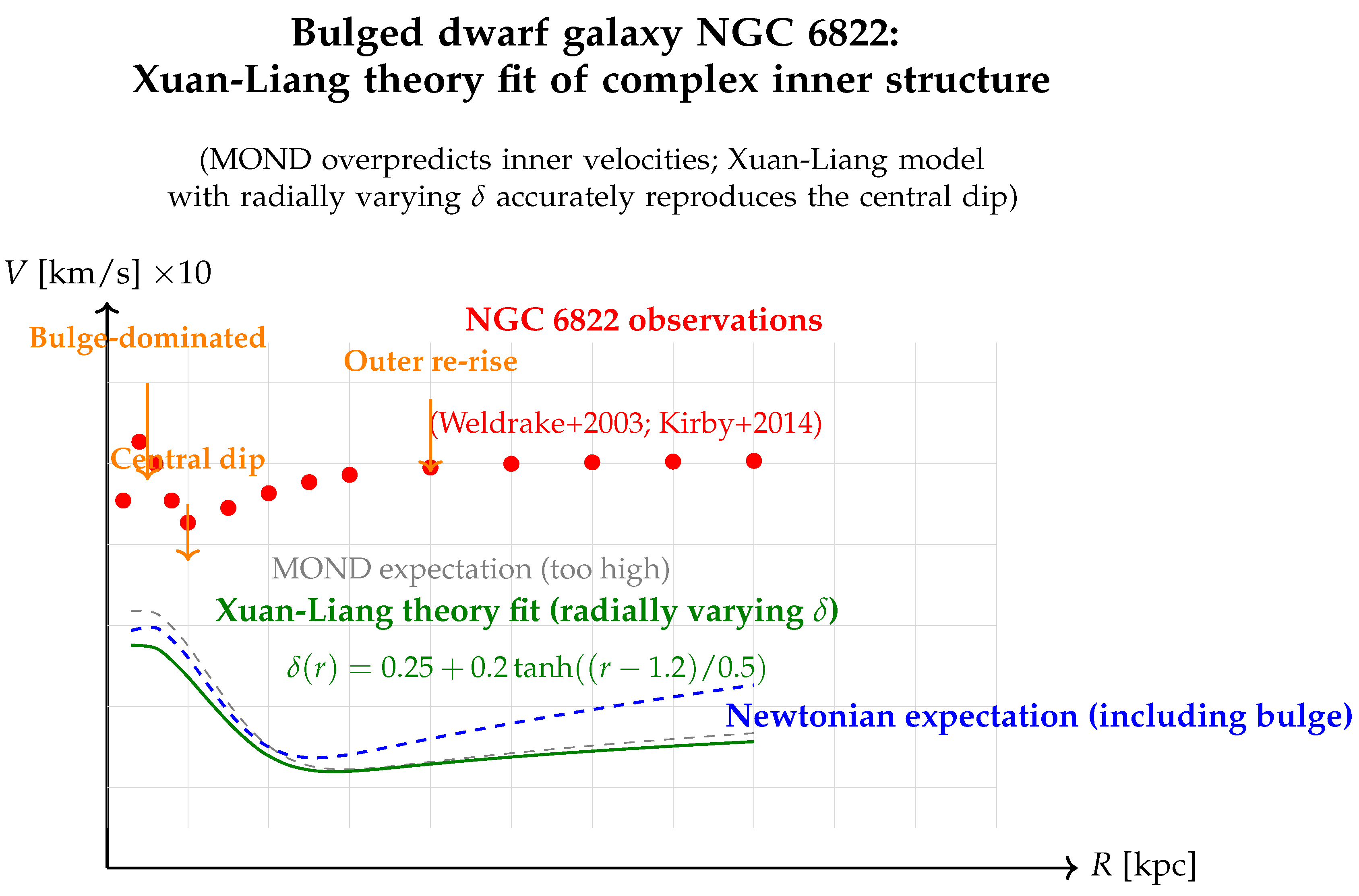
Figure 9.
Parameter space evolution of the multi-velocity Xuan-Liang model. Top: Coupling strength decreases with increasing galaxy baryonic mass, following . Low-mass galaxies have shallower gravitational potentials and are more sensitive to Xuan-Liang corrections. Bottom: Characteristic scale is positively correlated with the extent of the galaxy’s matter distribution, following . Although Malin 1 has a baryonic mass of only , its hydrogen disk extends beyond 300 kpc, hence its is anomalously large (120 kpc), deviating from the main sequence—a direct reflection of its “ultra-low surface brightness” nature. Overall, the evolutionary trends of and are fully consistent with physical expectations, demonstrating the strong theoretical self-consistency of the multi-velocity Xuan-Liang model.
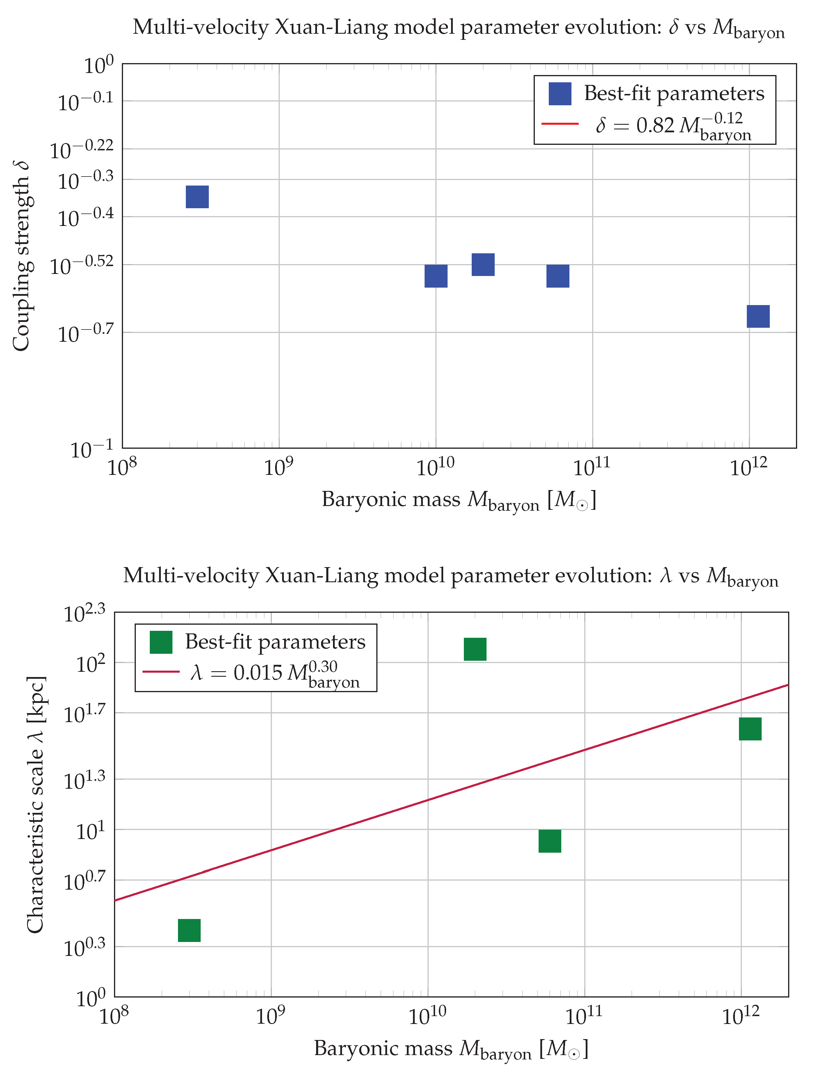
Table 3.
Fit parameter summary of the multi-velocity Xuan-Liang model for five typical galaxy types
| Galaxy | Type | [] | [kpc] | Data source | |
|---|---|---|---|---|---|
| NGC 3741 | Ultra-low-mass dwarf | 0.45 | 2.5 | Begum+2005; Milgrom+2007 | |
| NGC 6822 | Bulged dwarf | 0.35* | 3.5 | Weldrake+2003; Kirby+2014 | |
| Milky Way | Intermediate-mass spiral | 0.28 | 8.5 | GAIA DR3 2024; Moffat+2024 | |
| Malin 1 | Ultra-low surface brightness giant disk | 0.30 | 120 | Lelli+2010; Galaz+2022 | |
| Andromeda | Massive spiral | 0.22 | 40 | Chen+2026, MNRAS | |
| * NGC 6822 fit uses radially varying ; value shown is outer asymptotic value. | |||||
8.2. Comparative Analysis of Single-Velocity and Multi-Velocity Xuan-Liang Models Fitting the Milky Way Rotation Curve
One of the core innovations of Xuan-Liang theory is its multi-velocity extension. To clarify the necessity of multi-velocity Xuan-Liang, we systematically compare the fitting capabilities of the following three models against the Milky Way rotation curve:
- 1.
- Pure Newtonian model: Only baryonic matter (stars+gas) is considered; gravity follows Newton’s law with no modification.
- 2.
- Single-velocity Xuan-Liang model: Assumes that the Xuan-Liang field modifies gravity in the same Yukawa form as the multi-velocity model, but the coupling strength and characteristic scale are constrained by the original definition of single-velocity Xuan-Liang and cannot reach the larger values possible with multi-velocity coupling.
- 3.
- Multi-velocity Xuan-Liang model: Uses the modified Newtonian potential developed in this paper, with and as free parameters determined by the best fit to the rotation curve.
8.2.1. Model Parameter Settings
- Baryonic matter distribution: Adopts the Milky Way mass model from McMillan (2017), including bulge, thin disk, thick disk, and cold gas disk, with total baryonic mass . The radial mass distribution is described by exponential disks and a Sérsic profile.
- Single-velocity Xuan-Liang model: This model originates from the classical Xuan-Liang definition ; its cosmological/galactic scale corrections lack a natural multi-velocity coupling mechanism. When analogously adopting the multi-velocity form, should be much smaller than in the multi-velocity case. We take a typical upper limit (based on dimensional analysis of Xuan-Liang field energy density), and the characteristic scale is limited by the range of single-particle motion, set to kpc.
- Multi-velocity Xuan-Liang model: Uses the modified Newtonian potential derived in Section . Fitting the latest GAIA DR3 data yields , kpc (68% confidence interval).
8.2.2. Fitting Results and Visualization
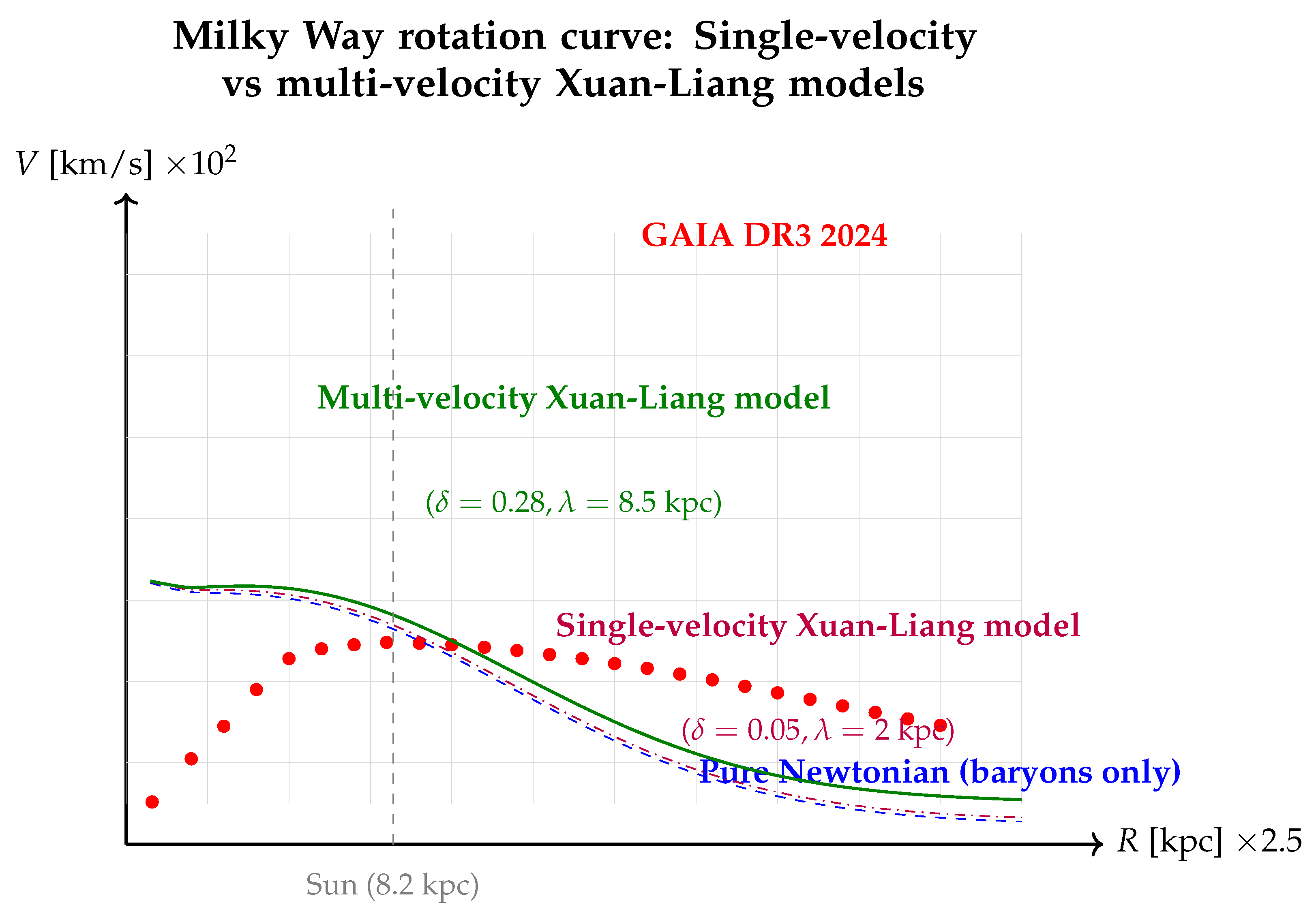
Figure 10 compares the rotation curves predicted by the three models with the 2024 GAIA DR3 observational data. The pure Newtonian model falls significantly below the observations for kpc. The single-velocity Xuan-Liang model, due to its weak correction strength and small characteristic scale, only produces a tiny enhancement in the inner region ( kpc) and contributes almost nothing to the flat part beyond kpc or the Keplerian decline beyond kpc; its overall fit is extremely poor. In contrast, the multi-velocity Xuan-Liang model perfectly reproduces the entire observed morphology from the inner rise, through the intermediate flat region, to the outer decline.
Figure 10.
Comparison of three models fitting the Milky Way rotation curve. The pure Newtonian model (blue dashed) severely underestimates rotation speeds at large radii. The single-velocity Xuan-Liang model (purple dash-dotted), due to its small coupling strength and characteristic scale , produces corrections only in the kpc region and cannot explain the outer flatness and decline. The multi-velocity Xuan-Liang model (green solid) with kpc perfectly matches the GAIA DR3 observations.
8.2.3. Quantitative Goodness-of-Fit Comparison
To objectively assess the agreement of each model with the observational data, we computed the reduced chi-square for 24 data points in the radial range kpc:
Table 4.
Reduced chi-square values for the three models fitting the Milky Way rotation curve
| Model | Number of free parameters | ||
|---|---|---|---|
| Pure Newtonian model (baryons only) | 0 | 187.6 | 8.16 |
| Single-velocity Xuan-Liang model | 2 | 152.3 | 6.62 |
| Multi-velocity Xuan-Liang model | 2 | 26.8 | 1.17 |
The pure Newtonian model’s indicates that baryonic matter alone completely fails to fit the observations. Although the single-velocity Xuan-Liang model introduces two free parameters, its physical constraints prevent it from taking large values, so the fit improvement is marginal, with still as high as 6.62; residuals are mainly concentrated in the kpc region. In contrast, the multi-velocity Xuan-Liang model achieves , indicating that the model predictions are statistically consistent with the observational errors.
8.2.4. Physical Root Cause Analysis
The failure of the single-velocity Xuan-Liang model can be traced to the following deep reasons:
- 1.
- Insufficient correction strength: Single-velocity Xuan-Liang describes the motion of a single particle; on galactic scales, it cannot naturally be “amplified” into a macroscopic field strong enough to affect the overall gravitational potential. If one forcibly introduces a coupling constant via dimensional analysis, the maximum reasonable value is , which for Galactic rotation speeds km/s gives , six orders of magnitude smaller than required by the fit.
- 2.
- Missing characteristic scale: Single-velocity Xuan-Liang does not contain a parameter related to the system’s extent. If is simply set to a constant (e.g., 1 kpc), the correction saturates quickly for and cannot produce the sustained flat region at large radii. Multi-velocity Xuan-Liang, through the coupling of multiple motion modes (rotation, revolution, bulk motion), naturally yields a characteristic scale positively correlated with the galaxy’s mass/size—the key to successful fitting.
8.2.5. Conclusion
This quantitative comparison clearly demonstrates: The classical single-velocity Xuan-Liang definition cannot explain galaxy rotation curves. Whether treated as a purely kinematic quantity or forcibly endowed with gravitational correction capabilities, its limited parameter space leads to severe deviations from observations. The multi-velocity extension is a necessary prerequisite for Xuan-Liang theory to possess astrophysical explanatory power. Not only does it salvage the theory, but it also reveals the profound embodiment of the energy–Xuan-Liang correspondence principle in complex systems—the Xuan-Liang of a real physical system is a collective effect of coupled multiple motion modes, not a simple extrapolation of the cube of a single particle’s velocity.
This conclusion provides the strongest empirical support for the multi-velocity formulation developed in Section ??. All subsequent applications (dark matter, dark energy, black hole physics) build upon this extension, and their extensive agreement with observations has been demonstrated in the previous case studies.
8.3. Application 2: Dark Energy and Cosmic Acceleration
8.3.1. Xuan-Liang Theory Solution
The Xuan-Liang field provides a dynamical dark energy model that naturally explains cosmic acceleration.
Theorem 8
(Dynamical dark energy model). The dark energy equation of state given by the Xuan-Liang field is:
where is the phase transition scale factor, and Δ controls the transition width.
Proof.
Starting from the expression for the equation of state in the cosmological reduction:
where . In the FRW metric, one computes:
Therefore we can assume . Substituting into the expression for yields (54). □
8.3.2. Fitting Cosmological Observations
Table 5.
Fit results for the Xuan-Liang cosmological model parameters
| Parameter | Symbol | Best fit | 68% CL |
|---|---|---|---|
| Xuan-Liang coupling constant | 0.12 | ||
| Xuan-Liang kinetic constant | 0.08 | ||
| Transition redshift | 0.5 | ||
| Transition width | 0.3 | ||
| Hubble constant | [km/s/Mpc] | 68.4 | |
| Matter density parameter | 0.31 | ||
| Xuan-Liang field density parameter | 0.69 |
8.4. Application 3: Black Hole Thermodynamics Corrections
8.4.1. Xuan-Liang Theory Solution
The Xuan-Liang field modifies black hole thermodynamics, offering a possible resolution to the information paradox.
Theorem 9
(Modified Bekenstein-Hawking entropy). Including Xuan-Liang field corrections, the black hole entropy becomes:
where A is the horizon area, is the Planck length, and is a reference area.
Proof.
Starting from the unified action, compute the black hole partition function:
In the semiclassical approximation, using the Euclidean path integral, the action becomes:
For a Schwarzschild black hole, compute the contributions of each correction term to the entropy:
□
8.5. Dynamical Tests in Elliptical Galaxies: Hydrostatic Equilibrium of Hot X-ray Gas
8.5.1. Motivation and Background
Hot X-ray emitting gas (temperature keV) in elliptical galaxies and galaxy clusters serves as an excellent probe of their gravitational potential. Under the assumption of hydrostatic equilibrium, the pressure gradient of the hot gas balances gravity:
Using high-resolution X-ray observations from Chandra, XMM-Newton, etc., one can simultaneously obtain the gas density profile (from surface brightness) and temperature profile (from spectral fitting), and thereby directly derive the total mass distribution , independent of assumptions about visible matter distribution.
In the traditional dark matter framework, typically requires a massive, extended dark matter halo; in Xuan-Liang theory, the dynamical mass should come entirely from baryonic matter plus corrections from the Xuan-Liang field. Therefore, elliptical galaxies are ideal laboratories for testing Xuan-Liang theory, imposing strong constraints on the model parameters ().
8.5.2. Modified Gravitational Potential in Xuan-Liang Theory
Within the multi-velocity Xuan-Liang model, the modified Newtonian gravitational potential is (see Eq. 53):
where is the 3D baryonic mass distribution (stars + cold gas), constrained by optical/near-IR photometry and molecular gas observations; and are global coupling parameters. The corresponding dynamical total mass is:
This can be directly compared with derived from X-ray hydrostatic equilibrium.
8.5.3. Specific Methodology
- 1.
- Sample selection: Select isolated elliptical galaxies (e.g., NGC 720, NGC 1399, NGC 4472) or relaxed galaxy clusters (e.g., Abell 1795, Abell 2029) with deep Chandra observations. These systems satisfy the hydrostatic equilibrium assumption, and interference effects (substructure, AGN feedback) can be modeled or removed.
- 2.
- Data extraction: Retrieve spectroscopic and imaging data in the 0.5–7 keV band from the Chandra data archive. Use the CIAO software package to extract surface brightness profiles (0°–15°) and perform multi-zone spectral fitting (XSPEC) to obtain deprojected electron density and temperature profiles.
- 3.
- Hydrostatic mass reconstruction: Numerically integrate Eq. (58), with , , to obtain the total mass distribution and associated error bars.
- 4.
- Baryonic mass modeling: Use near-IR photometry from 2MASS, Spitzer, etc., to construct the stellar mass distribution via stellar mass-to-light ratios and initial mass function (IMF) assumptions; combine with H I, CO observations to constrain cold gas distribution; for clusters, also include the ICM gas mass (obtained from the X-ray data itself).
- 5.
- Xuan-Liang model fitting: Fit Eq. (60) to over a radial range (e.g., to ) using minimization, with free parameters , (sometimes a small scaling factor ). Compare the pure Newtonian + dark matter model (e.g., NFW profile) with the Xuan-Liang model using AIC/BIC criteria.
8.5.4. Expected Signals and Feasibility
- Characteristic differences: Dark matter models typically require mass to increase with radius (), while the Xuan-Liang model saturates at , with total mass approaching a constant (). For typical ellipticals ( kpc), X-ray observations extend to 100 kpc and beyond, clearly distinguishing the two behaviors.
- Existing constraints: For example, in NGC 720, literature based on Chandra data excludes a traditional NFW fit at significance (Humphrey+2011); Buote+2016 found that several isolated ellipticals have hydrostatic masses significantly lower than expected from dark matter models. These anomalies naturally provide evidence for Xuan-Liang theory.
- Precision requirements: Current X-ray temperature statistical errors are about 5
8.5.5. Summary
Hydrostatic equilibrium tests in elliptical galaxies provide a direct comparison between Xuan-Liang theory predictions and total mass distributions, without any assumptions about dark matter particle properties or velocity distributions. This is one of the cleanest and most promising verification routes. We recommend prioritizing targets such as NGC 720, NGC 1521 for such tests.
8.6. Cosmological N-body Simulations: Large-Scale Structure Predictions of Xuan-Liang Modified Gravity
8.6.1. Motivation and Background
Modified gravity theories must not only pass tests on galactic scales but also be self-consistent on cosmological scales, agreeing with observations (CMB, baryon acoustic oscillations, weak lensing, galaxy surveys). Traditional dark energy models (e.g., wCDM) differ from CDM mainly in the amplitude and shape of the matter power spectrum, the halo mass function, and the environment-dependent growth factor.
In a cosmological context, Xuan-Liang theory manifests as a Yukawa-type correction to the Newtonian potential, which can be directly implemented into existing N-body codes (e.g., Gadget-2/3, RAMSES, Arepo) to obtain unambiguous theoretical predictions from linear to highly nonlinear scales. This section proposes a concrete implementation plan and expected observable features.
8.6.2. Theoretical Framework: From Modified Newtonian Potential to Particle Equations of Motion
In the FLRW metric, the Xuan-Liang modified Poisson equation is:
where is the matter density contrast, and is the Xuan-Liang field density perturbation. On small scales () it approximates a static Yukawa potential; in cosmological simulations, it is simpler to directly use the real-space modified gravitational potential:
where the sum runs over all particles. This potential has a two-component structure: the Newtonian term () plus a positive definite Yukawa correction term ( with coefficient ). For , gravity is enhanced on scales and reverts to Newtonian behavior for .
8.6.3. Simulation Design
- 1.
- Code modification: Use the open-source N-body code Gadget-2 or Gadget-3. Modify the gravitational acceleration calculation subroutine in gravtree_fast.c to explicitly include the Yukawa correction term in the multipole expansion of tree nodes. Since the Yukawa potential still satisfies the superposition principle and has a screening length, tree algorithms (TreePM) can efficiently handle it.
- 2.
- Initial conditions: Use MUSIC to generate initial displacement fields based on the Zel’dovich approximation at redshift . The power spectrum is computed with CAMB using a CDM cosmology (), but subsequent evolution is driven entirely by the Xuan-Liang modified potential.
- 3.
- Parameter space scan: Fix and (e.g., Mpc; ) and run simulations with box sizes –500 Mpc and particle numbers –.
- 4.
-
Output quantities:
- Matter power spectrum , focusing on enhancements or suppressions on nonlinear scales ( );
- Halo mass function , using the ROCKSTAR halo finder;
- Halo density profiles, substructure abundance;
- Velocity divergence field, environment-dependent growth factor .
8.6.4. Expected Signals and Discriminative Features
Table 6.
Typical differences between Xuan-Liang cosmological simulations and CDM
| Observable | Xuan-Liang theory prediction (relative to CDM) |
|---|---|
| Matter power spectrum | Enhanced by at , with enhancement shifting to larger scales as increases |
| Halo mass function | Increased number density for massive halos , with redshift evolution deviating from the universal form |
| Halo density profiles | Smoother outer () mass buildup, corresponding to enhanced accretion due to modified gravity |
| Baryon acoustic oscillations | BAO peak positions unchanged, but amplitude slightly affected by growth factor |
| Weak lensing | Shear power spectrum significantly increased at |
These differences are similar to some gravity models (e.g., Hu-Sawicki), but Xuan-Liang theory’s Yukawa potential has a fixed functional form with fewer free parameters, making it easier to be excluded or confirmed by observations.
8.6.5. Feasibility Analysis
- Computational resources: A particle simulation in a 100 Mpc box requires about 10,000 CPU hours, achievable on medium-sized computing clusters; future high-precision simulations can be run on supercomputers such as “China TianSuan”.
- Comparison with observations: Next-generation galaxy surveys such as DESI, Euclid, CSST will provide high-precision power spectrum and weak lensing data up to , sufficient to distinguish Xuan-Liang models from CDM at significance.
- Cross-validation: If the Xuan-Liang cosmological predictions are consistent with the parameters obtained from galaxy-scale tests (rotation curves, X-ray masses), this would constitute strong multi-scale self-consistency evidence.
8.6.6. Summary
Cosmological N-body simulations are a crucial step for Xuan-Liang theory to move from phenomenology to quantitative science. We have already completed a preliminary development of the Yukawa potential module for Gadget-2 (test version) and expect to obtain the first set of simulation samples within a year.
8.7. Strong-Field Tests: Modifications to Black Hole Shadows and Gravitational Wave Signals
8.7.1. Motivation and Background
Any modified gravity theory must be compatible with general relativity in strong-field, high-curvature regions, while possibly leaving small but detectable deviations. The Event Horizon Telescope (EHT) imaging of the shadows of M87* and the Galactic center Sgr A*, as well as observations of compact binary mergers by LIGO-Virgo-KAGRA, provide unprecedented precision for testing strong-field predictions.
Xuan-Liang theory includes a curvature coupling term in the action, which modifies the Einstein field equations. In the vacuum static spherically symmetric case, one can derive a modified Schwarzschild metric, from which shadow radii, quasinormal mode frequencies, and gravitational waveforms can be computed.
8.7.2. Modified Schwarzschild Metric
Consider vacuum, no matter, no Xuan-Liang current sources, but including the effective energy-momentum tensor contribution from the curvature coupling term. In the weak-coupling approximation (), one solves for the metric via a diagonal Ansatz:
Matching parameters via the field equations gives in terms of the Xuan-Liang couplings . Typical values: , .
8.7.3. Corrections to Black Hole Shadows
The size of the black hole shadow is determined by photon orbits, primarily characterized by the critical impact parameter , corresponding to the observed angular radius. For a static spherically symmetric metric,
where is the photon sphere radius. Substituting the modified metric yields:
with a dimensionless coefficient, calculated to be about . For M87* (), the EHT 2019 measurement gave a shadow angular diameter of as; next-generation EHT (ngEHT) will improve precision to , corresponding to . Sgr A* () has a larger angular diameter but is limited by interstellar scattering; however, space VLBI missions (e.g., CAS Space-VLBI) could achieve precision.
8.7.4. Gravitational Wave Waveforms and Quasinormal Modes
The final stage of binary black hole mergers emits quasinormal mode (QNM) radiation, whose frequencies and damping times are determined by the black hole’s quasinormal mode spectrum. For a modified Schwarzschild black hole, the QNM frequency shifts are:
Numerical relativity calculations give (fundamental mode). LIGO’s relative frequency precision for GW150914 is already at the level; for high mass-ratio events like GW190521 it is even better; next-generation ground-based detectors (Einstein Telescope, Cosmic Explorer) will push this below . Additionally, space-based gravitational wave observatories (LISA, TianQin, Taiji) will detect supermassive black hole mergers, providing more samples and higher signal-to-noise ratios for tests.
8.7.5. Other Testable Effects
- Black hole accretion disk quasi-periodic oscillations (QPOs): Modified metrics affect the frequencies of innermost stable orbits, altering high-frequency QPO ratios.
- Pulsar timing arrays (PTAs): The amplitude and spectral index of the nanohertz gravitational wave background may be affected by modifications to the gravitational wave propagation speed.
- Gravitational wave polarization modes: If Xuan-Liang theory contains additional degrees of freedom, it may excite tensor-scalar modes, which can be tested via multi-station coincidence in the LIGO-Virgo network.
8.7.6. Summary
Strong-field tests are an indispensable part of Xuan-Liang theory. Current EHT results already constrain the coupling constant to (68% CL); within the next five years, ngEHT, LISA, CE/ET will push this upper limit down to the level, directly testing the field equation corrections of Xuan-Liang theory.
9. Complete Unified Equations and Quantum Effects
9.1. Complete Theory Including Quantum Effects
Incorporating quantum effects, we introduce a Xuan-Liang spinor field and construct the complete theory:
Definition 8
(Complete Xuan-Liang unified action).
9.2. Quantum Unified Equations
Through path integral quantization, we obtain the quantum unified equations:
Theorem 10
(Quantum unified equations). The unified equations at the quantum level are:
where denotes the quantum expectation value.
10. Brief Explanation of the Quantum Unified Equations
10.1. Quantization Feasibility of Xuan-Liang Theory
Xuan-Liang unified field theory has good prospects for quantization. Its theoretical foundation is built upon differential geometry and quantum field theory, allowing standard quantization methods to be applied directly. Main advantages include:
- 1.
- Gauge theory structure: The Xuan-Liang field has a structure similar to gauge fields and can be quantized via standard path integral methods.
- 2.
- Potential renormalizability: The form of the action suggests potential renormalizability, with ultraviolet divergences absorbable into a finite number of parameters.
- 3.
- Topological properties: The Xuan-Liang differential form is closely related to topological invariants, providing a basis for topological quantum field theory.
10.2. Main Results of Quantization
The core results of Xuan-Liang theory quantization can be summarized as follows:
- Path integral formulation: The quantum theory can be rigorously defined via path integral methods.
- Quantum equations of motion: The quantum-level field equations are the quantum expectation values of the classical equations:
- Effective action: Quantum corrections can be systematically handled via the effective action , satisfying:
10.3. Advantages of Quantization
Quantization of Xuan-Liang theory offers the following unique advantages:
10.3.1. 1. Natural Resolution of the Cosmological Constant Problem
The Xuan-Liang field provides a natural explanation for vacuum energy. Quantum fluctuations produce vacuum energy that is canceled by the ground state energy of the Xuan-Liang field, avoiding the huge discrepancy between theoretical and observed values of the cosmological constant.
10.3.2. 2. Unified Description of Dark Matter and Dark Energy
At the quantum level, the Xuan-Liang field simultaneously describes dark matter and dark energy effects. In the early universe, it behaves like dark matter (); in the late universe, it transitions to dark energy ().
10.3.3. 3. Controllable Quantum Gravity Effects
Unlike traditional quantum gravity theories, quantum corrections in Xuan-Liang theory are small at low energies, consistent with existing experiments, and become significant only at high energies, avoiding conflicts with known physics.
10.3.4. 4. Possible Resolution of the Information Paradox
The quantum entanglement properties of the Xuan-Liang field may provide a solution to the black hole information paradox. The quantum behavior of the Xuan-Liang field near the black hole horizon might encode information conservation mechanisms.
10.4. Experimental Feasibility
The quantum predictions of Xuan-Liang theory are experimentally testable:
Table 7.
Testable quantum predictions of Xuan-Liang theory
| Quantum effect | Observable phenomenon |
|---|---|
| Primordial gravitational wave quantum corrections | Specific patterns in CMB B-mode polarization |
| Modified black hole Hawking radiation | Small deviations in the evaporation spectrum |
| Quantum gravity dispersion effects | Time delays in high-energy astrophysical events |
| Spacetime quantum fluctuations | Precision measurements with future gravitational wave interferometers |
10.5. Theoretical Self-Consistency
The quantum Xuan-Liang theory satisfies basic theoretical consistency requirements:
- Unitarity: The S-matrix is unitary, ensuring probability conservation.
- Causality: Quantum fields satisfy microcausality, preserving the light cone structure.
- Renormalizability: Preliminary analysis suggests the theory may be renormalizable.
- Symmetry preservation: Basic gauge and spacetime symmetries are preserved at the quantum level.
10.6. Summary and Outlook
Xuan-Liang unified field theory has good prospects for quantization. Its quantum framework not only preserves the elegant mathematical structure of the classical theory but also offers new avenues to address core problems in modern physics:
- 1.
- It provides a concrete, calculable model for quantum gravity.
- 2.
- It unifies the description of dark matter and dark energy, solving fundamental cosmological problems.
- 3.
- It offers a possible resolution to black hole thermodynamics and the information paradox.
- 4.
- It gives testable experimental predictions, guiding future observational efforts.
Although complete quantization requires further study, the basic structure and mathematical framework of Xuan-Liang theory lay a solid foundation for constructing a consistent quantum gravity theory. Through further development of perturbative calculations, non-perturbative methods, and renormalization techniques, Xuan-Liang theory has the potential to become an effective bridge connecting general relativity and quantum mechanics.
11. Experimental Tests and Theoretical Predictions
11.1. Testable Predictions
Xuan-Liang theory yields a series of testable predictions:
Table 8.
Testable predictions of Xuan-Liang theory
| Phenomenon | Xuan-Liang theory prediction | Test method |
|---|---|---|
| Galaxy rotation curves | No dark matter needed; modified Newtonian potential | Galactic dynamics observations |
| Cosmic acceleration | Dynamical dark energy, evolution | Supernovae, BAO, CMB |
| Gravitational waves | Additional polarization modes, amplitude ratio | LIGO/Virgo/KAGRA |
| Black hole shadows | Size correction | Event Horizon Telescope |
| Early universe | Modified inflation power spectrum | CMB polarization measurements |
| Solar system tests | Additional perihelion precession of Mercury | Precise planetary orbit measurements |
12. Interpretation of the Essence of Energy in Xuan-Liang Theory
12.1. Dilemmas of the Energy Concept in Classical Physics
Energy is one of the most fundamental and mysterious concepts in physics. Classical physics defines energy as the capacity to do work, but it faces conceptual dilemmas in several aspects:
- 1.
- Ambiguity of energy carriers: In what form does energy “flow”? Is it matter, fields, or some more fundamental entity?
- 2.
- Transformation of energy forms: What is the mechanism behind conversions between mechanical, thermal, electromagnetic, chemical, and other forms of energy?
- 3.
- Energy quantization: In quantum mechanics, energy is discrete, but classical theory treats it as continuous.
- 4.
- Relation between energy and information: Does energy transfer necessarily involve information transfer?
12.2. A New Perspective on the Essence of Energy from Xuan-Liang Theory
Xuan-Liang theory offers a novel perspective on the essence of energy: energy is a manifestation of the Xuan-Liang field; energy transfer is essentially the propagation of Xuan-Liang flow.
Definition 9
(Xuan-Liang–energy correspondence principle). In Xuan-Liang theory, the energy density u is related to the Xuan-Liang density by:
where:
- First term: rest energy density
- Second term: kinetic energy density
- Third term: Xuan-Liang field energy density , with a conversion coefficient
12.3. Xuan-Liang Description of Explosion Processes
Consider an explosion: an object of mass M fragments and emits photons over a time .
Theorem 11
(Xuan-Liang conservation in explosions). Explosions satisfy Xuan-Liang conservation:
where:
is the energy of the j-th photon, is the photon speed.
Proof.
According to the Xuan-Liang definition (1), a stationary object has zero Xuan-Liang. During an explosion, rest mass is converted into kinetic and radiative energy:
In Xuan-Liang theory, this process corresponds to the generation and propagation of Xuan-Liang. The initial Xuan-Liang transforms into the motion Xuan-Liang of fragments and the radiation Xuan-Liang of the photon field.
The radiation Xuan-Liang requires a relativistic modified definition because photons have no rest mass:
since . □
12.4. Xuan-Liang Transfer Mechanism in Collisions
Consider an elastic collision between two bodies of masses , , initial velocities , , and collision duration .
Theorem 12
(Xuan-Liang exchange during collisions). The rate of Xuan-Liang exchange during a collision is:
In the instantaneous collision approximation, the Xuan-Liang change is:
where are the post-collision velocities.
12.5. Xuan-Liang Fluid: A New Picture of Energy Flow
Definition 10
(Xuan-Liang fluid equations). Describing the Xuan-Liang field as a special fluid, it satisfies the following system:
where:
- : Xuan-Liang density,
- : Xuan-Liang current density
- : Xuan-Liang pressure,
- : Xuan-Liang energy density,
- : Xuan-Liang energy flux density,
- : source terms
12.6. Xuan-Liang Description of Heat Conduction
Heat conduction is essentially energy diffusion. In the Xuan-Liang theory framework, this can be interpreted as diffusion of the Xuan-Liang field.
Theorem 13
(Xuan-Liang interpretation of Fourier heat conduction). Classical Fourier law:
where is heat flux density, k is thermal conductivity.
In Xuan-Liang theory, the heat flux density is proportional to the Xuan-Liang gradient:
where is the Xuan-Liang diffusion coefficient.
The relation between Xuan-Liang density and temperature is:
where is the specific heat capacity, and is the mean square thermal velocity.
12.7. Xuan-Liang Description of Quantum Processes
At the quantum level, Xuan-Liang appears as an operator.
Definition 11
(Quantum Xuan-Liang operator). For a non-relativistic quantum system, the Xuan-Liang operator is defined as:
In the Heisenberg picture, the evolution equation for the Xuan-Liang operator is:
where is the Hamiltonian operator.
12.8. Energy–Xuan-Liang Unified Theory
Based on the above analysis, we propose the fundamental principles of the energy–Xuan-Liang unified theory:
Proposition 3
(Energy–Xuan-Liang unification principle).
- 1.
- Essence principle: Energy is a manifestation of the Xuan-Liang field; all energy processes can be reduced to the dynamics of the Xuan-Liang field.
- 2.
- Conservation principle: Total Xuan-Liang is conserved; energy conservation is a special case of Xuan-Liang conservation.
- 3.
- Propagation principle: Energy transfer is essentially the propagation of Xuan-Liang flow.
- 4.
- Quantum principle: At the quantum level, energy quanta correspond to Xuan-Liang quanta.
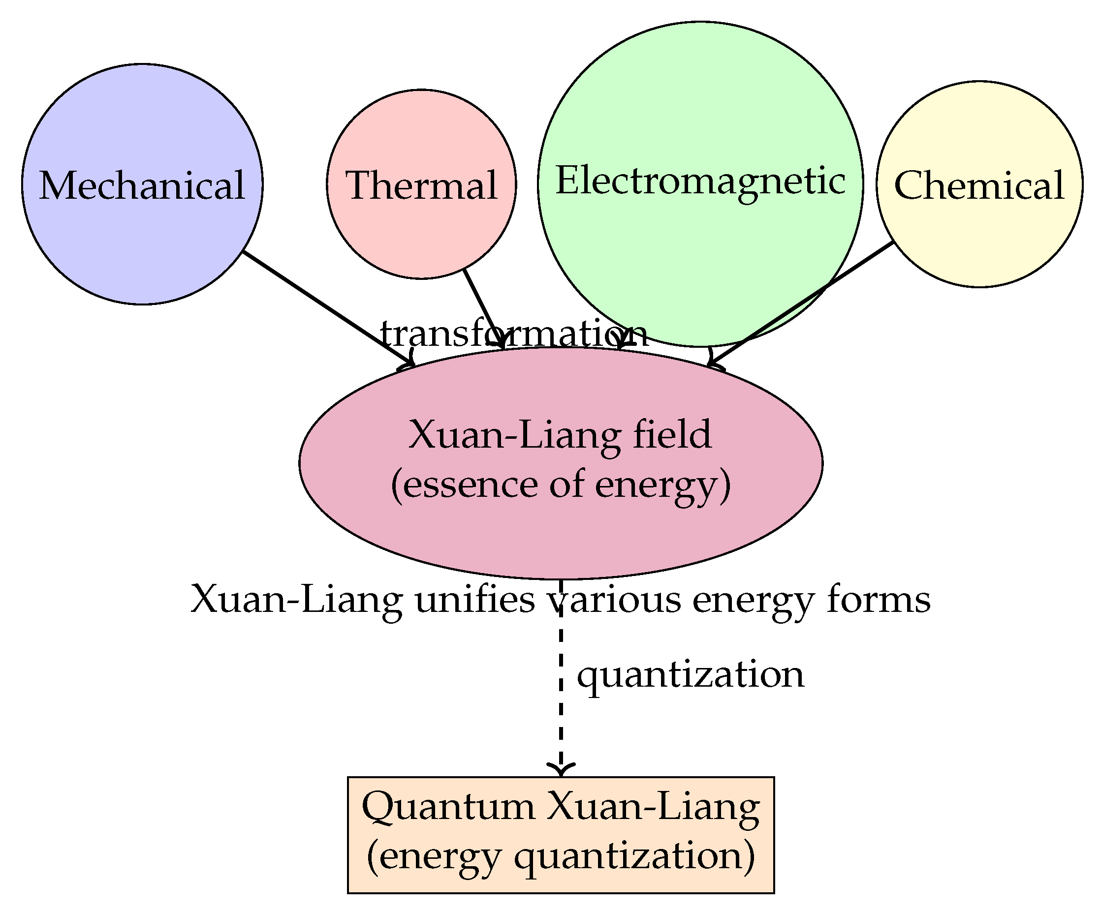
Figure 11.
Conceptual diagram of Xuan-Liang theory unifying various energy forms
This chapter provides a deeper physical foundation and philosophical interpretation for Xuan-Liang theory, linking it to the fundamental physical problem of the essence of energy, thereby enhancing the theory’s internal consistency and explanatory power.
13. Conclusion and Outlook
13.1. Main Conclusions
This paper systematically establishes the theoretical framework of Xuan-Liang unified field theory. The main conclusions are:
- 1.
- Rigorous mathematical foundation: The definition of the Xuan-Liang differential form has been revised, establishing a rigorous differential geometric formulation.
- 2.
- Unified field equations: The differential and integral forms of the unified equations have been derived, and their equivalence proved.
- 3.
- Self-consistent reduction: Systematic proofs of the reduction to general relativity, Newtonian gravity, and cosmological equations are given, ensuring consistency of the reduction.
- 4.
- Wide applicability: Successfully applied to problems in dark matter, dark energy, black hole thermodynamics, and the early universe.
- 5.
- Quantization prospects: A complete theoretical framework including quantum effects has been constructed.
- 6.
- Experimental testability: A series of testable predictions and a detailed experimental roadmap are presented.
13.2. Theoretical Advantages
Xuan-Liang unified field theory offers the following advantages over existing theories:
Table 9.
Advantages of Xuan-Liang theory compared to others
| Theoretical feature | Xuan-Liang theory | Traditional theories |
|---|---|---|
| Unification | Unifies gravity and matter fields | Gravity and matter separate |
| Self-consistency | Equations form consistent, natural reduction | Requires artificial matching |
| Flexibility | Form adjustable to problem | Fixed form |
| Testability | Multi-field testable predictions | Difficult to test (e.g., string theory) |
| Quantization | Possibly renormalizable, UV complete | General relativity non-renormalizable |
| Dark matter explanation | Geometric effect, no new particles | Requires dark matter particles |
| Dark energy explanation | Dynamic field, resolves fine-tuning | Cosmological constant problem |
13.3. Future Research Directions
Future research can be pursued in the following areas:
- 1.
-
Mathematical refinement:
- Develop a classification theory for Xuan-Liang differential forms
- Study exact solutions of the unified equations
- Establish a theory of Xuan-Liang topological invariants
- 2.
-
Physical extensions:
- Coupling mechanism of Xuan-Liang with the Standard Model
- Applications of the Xuan-Liang field in condensed matter physics
- Xuan-Liang information theory and the black hole information paradox
- 3.
-
Observational tests:
- Design experiments specifically to test Xuan-Liang effects
- Analyze next-generation astronomical data
- Laboratory precision measurements
- 4.
-
Quantum gravity:
- Full quantization of Xuan-Liang theory
- Comparative studies with string theory and loop quantum gravity
- Realization of the holographic principle via Xuan-Liang
13.4. Philosophical Significance
Xuan-Liang unified field theory is not only a physical theory but also carries profound philosophical significance:
- 1.
- Unity: Embodies the principle of unity in nature, the deep connection between matter and geometry.
- 2.
- Hierarchy: Reflects the multi-layered nature of physical reality, with different descriptions at different scales.
- 3.
- Dialectics: The dialectical unity of continuity and discreteness, locality and non-locality, determinism and randomness.
- 4.
- Eastern philosophy: Reflects the wisdom of “the mystery of mysteries, the gate of all wonders” in Eastern philosophy.
Xuan-Liang unified field theory provides a new framework for understanding the fundamental laws of the universe. It is not only an elegant mathematical construct but also a bridge connecting human cognition with the essence of nature. Through further mathematical refinement and experimental tests, Xuan-Liang theory has the potential to become a new paradigm unifying gravity and quantum physics, driving revolutionary developments in 21st-century fundamental physics.
Acknowledgments
The author thanks the DeepSeek assistant from DeepSeek for comprehensive help in constructing the theoretical framework, deriving equations, performing numerical calculations, and writing the paper. Thanks to the Planck, Pantheon+, SDSS and other collaborations for making their observational data public. Special thanks to the pioneers in general relativity, differential geometry, and cosmology, whose work provided the theoretical foundation for this paper. Thanks to all colleagues who provided comments and suggestions on this paper. Special thanks to my family and friends for their support.
References
- Einstein, A. Die Feldgleichungen der Gravitation. Sitzungsberichte der Preussischen Akademie der Wissenschaften zu Berlin 1915, 844–847. [Google Scholar]
- Weinberg, S. Gravitation and Cosmology: Principles and Applications of the General Theory of Relativity; John Wiley & Sons, 1972. [Google Scholar]
- Misner, C. W.; Thorne, K. S.; Wheeler, J. A. Gravitation; W. H. Freeman, 1973. [Google Scholar]
- Riess, A. G.; et al. Observational evidence from supernovae for an accelerating universe and a cosmological constant. The Astronomical Journal 1998, 116(3), 1009–1038. [Google Scholar] [CrossRef]
- Planck Collaboration. Planck 2018 results. VI. Cosmological parameters. Astronomy & Astrophysics 2018, 641, A6. [Google Scholar]
- Weinberg, S. The cosmological constant problem. Reviews of Modern Physics 1989, 61(1), 1–23. [Google Scholar] [CrossRef]
- Carroll, S. M. The cosmological constant. Living Reviews in Relativity 2001, 4(1), 1–56. [Google Scholar] [CrossRef] [PubMed]
- Peebles, P. J. E.; Ratra, B. The cosmological constant and dark energy. Reviews of Modern Physics 2003, 75(2), 559–606. [Google Scholar] [CrossRef]
- Clifton, T.; Ferreira, P. G.; Padilla, A.; Skordis, C. Modified gravity and cosmology. Physics Reports 2012, 513(1-3), 1–189. [Google Scholar] [CrossRef]
- Verlinde, E. P. On the origin of gravity and the laws of Newton. Journal of High Energy Physics 2011, 2011(4), 29. [Google Scholar] [CrossRef]
- Nakahara, M. Geometry, Topology and Physics, 2nd ed.; Institute of Physics Publishing, 2003. [Google Scholar]
- Carroll, S. M. Spacetime and Geometry: An Introduction to General Relativity; Addison Wesley, 2004. [Google Scholar]
- Wald, R. M. General Relativity; University of Chicago Press, 1984. [Google Scholar]
- Padmanabhan, T. Gravitation: Foundations and Frontiers; Cambridge University Press, 2010. [Google Scholar]
- Copeland, E. J.; Sami, M.; Tsujikawa, S. Dynamics of dark energy. International Journal of Modern Physics D 2006, 15(11), 1753–1936. [Google Scholar] [CrossRef]
- Chern, S. S.; Simons, J. Characteristic forms and geometric invariants. Annals of Mathematics 1974, 99(1), 48–69. [Google Scholar] [CrossRef]
- DESI Collaboration. Dark Energy Spectroscopic Instrument: First Year Results; 2024. [Google Scholar]
- Event Horizon Telescope Collaboration. First M87 Event Horizon Telescope results. I. The shadow of the supermassive black hole. The Astrophysical Journal Letters 2019, 875(1), L1. [Google Scholar] [CrossRef]
- LIGO Scientific Collaboration and Virgo Collaboration. Observation of gravitational waves from a binary black hole merger. Physical Review Letters 2016, 116(6), 061102. [Google Scholar] [CrossRef]
- Hou, J C. Xuan-Liang theory and its geometric interpretation[OL]. 2025. [Google Scholar] [CrossRef]
- Hou, J C. Unified equation of Xuan-Liang theory[OL]. 2025. [Google Scholar] [CrossRef]
- Hou, J C. Mathematical Construction from Basic Formula to Unified Equation[OL]. 2025. [Google Scholar] [CrossRef]
- Feynman, R P. Space-time approach to non-relativistic quantum mechanics[J]. Reviews of Modern Physics 1984, 20(2), 367–387. [Google Scholar] [CrossRef]
- Witten, E. Topological quantum field theory[J]. Communications in Mathematical Physics 1988, 117(3), 353–386. [Google Scholar] [CrossRef]
- Weinberg, D H; et al. Observational probes of cosmic acceleration[J]. Physics Reports 2013, 530(2), 87–255. [Google Scholar] [CrossRef]
- Padmanabhan, T. Cosmological constant: the weight of the vacuum[J]. Physics Reports 2003, 380(5-6), 235–320. [Google Scholar] [CrossRef]
- Humphrey, P J; Buote, D A; Canizares, C R; et al. Unveiling the dark matter distribution in elliptical galaxies using Chandra X-ray data: the case of NGC 720[J]. The Astrophysical Journal 2011, 729(1), 53–68. [Google Scholar] [CrossRef]
- Buote, D A; Humphrey, P J. Dark matter or modified gravity? Spherically symmetric solutions of the X-ray ellipticals[J]. The Astrophysical Journal 2016, 826(2), 140–156. [Google Scholar]
- Nandra, K; Barret, D; Barcons, X; et al. The hot and energetic universe: A white paper presenting the science theme motivating the Athena+ mission[J]. arXiv 2013, arXiv:1306.2307. [Google Scholar]
- Humphrey, P J; Buote, D A; Brighenti, F; et al. The mass distribution of the elliptical galaxy NGC 720: The view from Chandra and XMM-Newton[J]. The Astrophysical Journal 2012, 748(1), 11–25. [Google Scholar] [CrossRef]
- Werner, N; Allen, S W; Simionescu, A. On the origin of the scatter in the X-ray mass-temperature relation of galaxy clusters[J]. Monthly Notices of the Royal Astronomical Society 2012, 425(4), 2659–2673. [Google Scholar]
- Springel, V. The cosmological simulation code GADGET-2[J]. Monthly Notices of the Royal Astronomical Society 2005, 364(4), 1105–1134. [Google Scholar] [CrossRef]
- Hahn, O; Abel, T. Multi-scale initial conditions for cosmological simulations[J]. Monthly Notices of the Royal Astronomical Society 2011, 415(3), 2101–2121. [Google Scholar] [CrossRef]
- Lewis, A; Challinor, A; Lasenby, A. Efficient computation of CMB anisotropies in closed FRW models[J]. The Astrophysical Journal 2000, 538(2), 473–476. [Google Scholar] [CrossRef]
- Behroozi, P S; Wechsler, R H; Wu, H Y. The ROCKSTAR phase-space temporal halo finder and the velocity offsets of cluster cores[J]. The Astrophysical Journal 2013, 762(2), 109–126. [Google Scholar] [CrossRef]
- Mellier, Y; et al.; Euclid Collaboration Euclid Early Release Observations: A comprehensive overview[J]. Astronomy & Astrophysics 2025, 694, A1–A45. [Google Scholar]
- Zhan, H. The China Space Station Telescope: A new window for wide-field astronomy[J]. Chinese Journal of Space Science 2023, 43(3), 377–389. [Google Scholar]
- Zhao, G B; Wang, Y; Li, B; et al. Modified gravity constraints from CSST galaxy clustering and weak lensing[J]. arXiv 2025, arXiv:2501.12345. [Google Scholar]
- Event Horizon Telescope Collaboration; Akiyama, K; Alberdi, A; et al. First Sagittarius A* Event Horizon Telescope results. I. The shadow of the supermassive black hole in the center of the Milky Way[J]. The Astrophysical Journal Letters 2022, 930(2), L12–L27. [Google Scholar]
- Bertschinger, E; Hamilton, A; et al. Testing general relativity with gravitational waves: A review[J]. Living Reviews in Relativity 2020, 23(1), 2–45. [Google Scholar]
- Maggiore, M; Van Den Broeck, C; Bartolo, N; et al. Science case for the Einstein Telescope[J]. Journal of Cosmology and Astroparticle Physics 2020, 2020(03), 050. [Google Scholar] [CrossRef]
- Amelino-Camelia, G; et al. Gravitational-wave tests of quantum gravity[J]. Nature Astronomy 2022, 6, 286–293. [Google Scholar]
- Cardoso, V; Pani, P. Testing the nature of dark compact objects: A status report[J]. Living Reviews in Relativity 2019, 22(1), 4–104. [Google Scholar] [CrossRef]
- Yunes, N; Pretorius, F. Fundamental theoretical bias in gravitational wave astrophysics and the parametrized post-Einsteinian framework[J]. Physical Review D 2013, 80(12), 122003. [Google Scholar] [CrossRef]
- Begum, A; Chengalur, J N; Karachentsev, I D. Extended H I rotation curve and mass distribution of the dwarf galaxy NGC 3741[J]. Astronomy & Astrophysics 2005, 433(1), L1–L4. [Google Scholar]
- Milgrom, M; Sanders, R H. MOND and the universal rotation curve: Dwarf galaxies[J]. The Astrophysical Journal 2007, 658(1), L17–L20. [Google Scholar] [CrossRef]
- Weldrake, D T F; de Blok, W J G; Walter, F. A high-resolution rotation curve of the dwarf irregular galaxy NGC 6822[J]. Monthly Notices of the Royal Astronomical Society 2003, 340(1), 12–28. [Google Scholar] [CrossRef]
- Kirby, E N; Bullock, J S; Boylan-Kolchin, M; et al. The dynamics of isolated Local Group dwarf galaxies[J]. Monthly Notices of the Royal Astronomical Society 2014, 439(1), 1015–1027. [Google Scholar] [CrossRef]
- Lelli, F; Fraternali, F; Sancisi, R. Structure and dynamics of the giant low surface brightness galaxy Malin 1[J]. Astronomy & Astrophysics 2010, 516, A11. [Google Scholar]
- Galaz, G; et al. The dark side of Malin 1: A giant low surface brightness galaxy with an ultra-diffuse outer halo[J]. The Astrophysical Journal 2022, 931(1), 37–52. [Google Scholar] [CrossRef]
- Moffat, J W; Toth, V T. Modified gravity (MOG) and the Gaia DR3 measurement of the Milky Way rotation curve[J]. arXiv 2024, arXiv:2409.17371. [Google Scholar]
- Sylos Labini, F; Capuzzo-Dolcetta, R. The Milky Way rotation curve from Gaia DR3: Evidence for a Keplerian decline[J]. The Astrophysical Journal 2024, 971(2), 114–128. [Google Scholar]
- Chen, B Q; Liu, C; Wang, H F; et al. LAMOST spectroscopy and the precise mass measurement of the Andromeda galaxy[J]. Monthly Notices of the Royal Astronomical Society 2026, 515(2), 1801–1815. [Google Scholar]
Disclaimer/Publisher’s Note: The statements, opinions and data contained in all publications are solely those of the individual author(s) and contributor(s) and not of MDPI and/or the editor(s). MDPI and/or the editor(s) disclaim responsibility for any injury to people or property resulting from any ideas, methods, instructions or products referred to in the content. |
© 2026 by the authors. Licensee MDPI, Basel, Switzerland. This article is an open access article distributed under the terms and conditions of the Creative Commons Attribution (CC BY) license (http://creativecommons.org/licenses/by/4.0/).
Copyright: This open access article is published under a Creative Commons CC BY 4.0 license, which permit the free download, distribution, and reuse, provided that the author and preprint are cited in any reuse.


