Soft Model Selection and Structured Assembly of Observables for Micro–Macro Transitions, Operational Relativity, and Emergent Thermodynamics

1. Motivation, positioning, and scope

“Essentially, all models are wrong, but some are useful.”

— George E. P. Box [1]

This manuscript does not propose a new physical theory, nor does it claim to unify quantum mechanics, classical dynamics, relativity, and thermodynamics at the level of a single state space. Instead, it proposes an operational meta-model that assembles predictions in a shared observable space. The contribution is therefore methodological: a disciplined way to combine existing regime-specific models, quantify confidence through soft weights, and detect when the available model catalog is insufficient.

Contributions (Incremental, Operational)

The contributions are modest and practical:

• A common observable space $\mathcal{Y}$ is formalized via a feature map $\Phi$, and regime transitions are treated as decisions in $\mathcal{Y}$ (rather than forcing incompatible state spaces into a single master model).
• A standard entropically-regularized soft selection rule (softmax/Gibbs form) is used to obtain convex weights from losses, augmented with a complexity penalty to mitigate overfitting.
• A small set of physics-inspired knobs (decoherence/classicality, relativistic severity, thermodynamicity) is used as operational priors that bias weights toward plausible regimes.
• A simple out-of-catalog diagnostic (surprise/residual monitoring) is proposed to flag when the chosen $\Phi$ and the candidate model set fail to explain data.

Relation to Prior Work

The weighting mechanism is closely related to well-known ideas such as Bayesian model averaging, Gibbs posteriors/PAC-Bayes methods, and mixture-of-experts gating. The goal is not to replace these frameworks, but to provide an explicit physics-facing operational interface: (i) a shared observable space $\mathcal{Y}$ tailored to measurement constraints, (ii) regime priors encoded by calibrated knobs, and (iii) a simple diagnostic for model-set inadequacy. In this sense, the novelty is primarily in the packaging and operationalization for micro–macro and regime-transition problems.

Scope and Limitations

This framework is only as good as (a) the chosen observable map $\Phi$ and (b) the candidate model catalog. The knobs $(\xi ,r,\theta )$ are not fundamental constants; they are operational summaries that must be calibrated for each experimental context. Accordingly, the method should be read as a principled decision layer on top of existing models, not as a substitute for domain-specific mechanistic modeling.

2. Level of Unification: the Output Space $\mathcal{Y}$ and the Map $\Phi$

Let X be the vector of observables to be predicted. Each formalism ${\mathcal{M}}_i$ produces a natural object $Z_i$ (trajectory, distribution, spectrum, quantum channel, etc.). A feature map is defined as

$$\Phi :\mathcal{Z}\to \mathcal{Y},{\widehat{X}}_i:=\Phi \left(Z_i\right)\in \mathcal{Y}.$$

Typical examples:

• $\Phi \left(P\right)=(\mu ,{\sigma }^2,{\kappa }_3,\dots ,{\kappa }_m)$ for a distribution P.
• $\Phi \left(S\right)=(S\left({\omega }_1\right),\dots ,S\left({\omega }_m\right))$ for a sampled spectrum.
• $\Phi \left(C\right)=(C\left({\tau }_1\right),\dots ,C\left({\tau }_m\right))$ for sampled correlations.

In practice, $\mathcal{Y}\approx {\mathbb{R}}^m$.

2.1. The Choice of $\mathcal{Y}$ is not Neutral (an Explicit Operational Hypothesis)

Selecting $\Phi$ and $\mathcal{Y}$ encodes which degrees of freedom are considered relevant in the micro–macro transition. In that sense, the coarse-graining implicit in $\Phi$ is an operational hypothesis: it assumes that certain functionals (moments, spectra, correlations) capture what is essential for the regime of interest. This choice should be guided by invariances, scales, and measurement constraints.

3. Assembly: Convex Combination and Structure-Preserving Operators

3.1. Base Meta-Predictor (Convex)

A minimal assembler is defined by

$$\widehat{X}=\sum _i{k}_i{\widehat{X}}_i,\sum _i{k}_i=1,k_i\ge 0.$$

(1)

3.2. Structured assembly (when constraints exist)

When the observable has structure (e.g., normalized distributions, PSD matrices, density matrices), a naive linear combination may violate constraints (positivity, normalization, etc.). In such cases, a structure-preserving assembly operator is used:

$$\widehat{X}=\mathcal{A}(\left\{{\widehat{X}}_i\right\},\mathbf{k}),$$

(2)

where $\mathcal{A}$ is chosen to preserve structure. Examples:

• Distributions: convex mixture in the probability simplex (preserves normalization and non-negativity).
• Density matrices: convex mixture of states $\rho ={\sum }_i{k}_i{\rho }_i$ (preserves positivity and trace 1).
• Constrained observables: projection $\Pi$ onto a valid convex set: $\widehat{X}=\Pi \left({\sum }_i{k}_i{\widehat{X}}_i\right)$.

Equation (1) is used as the minimal reference, and (2) as its natural extension.

4. Weights from Loss: Soft Selection with Regularization and Complexity

Let $E_i\ge 0$ be a total loss associated with model i. Define:

$$k_i={\displaystyle \frac{exp(-\lambda E_i)}{{\sum }_{j}exp(-\lambda E_j)}},\lambda >0.$$

(3)

4.1. Convex Interpretation (Minimum Loss + Entropy)

Rule (3) solves

$$\underset{k\in \Delta }{min}\sum _i{k}_i{E}_i+{\displaystyle \frac{1}{\lambda }}\sum _i{k}_{i}ln{k}_i,$$

(4)

where $\Delta =\{k_i\ge 0,{\sum }_i{k}_i=1\}$ and the second term is entropic regularization.

4.2. Loss Definition in $\mathcal{Y}$

If a reference $X^{★}$ exists (measurement or “fine” simulation),

$$E_i^{\mathrm{data}}=d({\widehat{X}}_i,X^{★}).$$

Common examples:

$$d_{\mathrm{RMSE}}(a,b)=\sqrt{{\displaystyle \frac{1}{m}}\sum _{\ell =1}^m{(a_{\ell }-b_{\ell })}^2},d_{\mathrm{KL}}(P\parallel Q)=\sum _{x}P\left(x\right)ln{\displaystyle \frac{P\left(x\right)}{Q\left(x\right)}}.$$

4.3. Complexity Penalty (AIC/BIC/MDL)

To reduce bias toward overly complex models,

$$E_i=E_i^{\mathrm{data}}+\beta {\Omega }_i,$$

(5)

where ${\Omega }_i$ can be AIC/BIC/MDL [2,3,4].

4.4. Knobs as Calibrated Parametrizations

The functional forms used for $(\xi ,r,\theta )$ are chosen for monotonicity, boundedness, and numerical stability. Other monotone parametrizations would be equally valid. In applications, these mappings should be calibrated (or learned) from validity data, measurement noise levels, and known scale separations.

5. Physics-Facing Priors from Knobs

Define dimensionless knobs (examples; operational use only):

$$\xi =\Gamma t_{\mathrm{obs}}(\mathrm{decoherence}/\mathrm{classicality}),$$

(6)

$${\beta }_S={\displaystyle \frac{v^2}{c^2}},{\beta }_G={\displaystyle \frac{2GM}{r{c}^2}},r=1-exp[-({\beta }_S+{\beta }_G)](\mathrm{relativistic}\mathrm{severity}),$$

(7)

$$\theta ={\displaystyle \frac{t_{\mathrm{obs}}}{{\tau }_{\mathrm{mix}}}}{N}_{\mathrm{eff}}\left(\mathrm{thermodynamicity}\right).$$

(8)

Let $q=e^{-\xi }$. A minimal factorized prior is:

$$w_{QR}=qr,w_Q=q(1-r),w_R=(1-q)r,w_C=(1-q)(1-r),$$

(9)

with $\sum w_{·}=1$.

5.1. Combining Prior + Loss

$$k_i={\displaystyle \frac{w_{i}exp(-\lambda E_i)}{{\sum }_j{w}_{j}exp(-\lambda E_j)}}.$$

(10)

6. Hardening: Knob Coupling and Out-of-Catalog Monitoring

6.1. Coupling Among Knobs (Validity Covariance)

Knobs $(\xi ,r,\theta )$ are often correlated in real systems. Let $\mathbf{p}:={(\xi ,r,\theta )}^{\top }$ and introduce a covariance matrix ${\Sigma }_{\mathbf{p}}\succ 0$. A Mahalanobis-type penalty is defined by

$$E_{\mathrm{cpl}}\left(\mathbf{p}\right):={\displaystyle \frac{1}{2}}{(\mathbf{p}-\mu )}^{\top }{\Sigma }_{\mathbf{p}}^{-1}(\mathbf{p}-\mu ),$$

(11)

where $\mu$ is an operational center (possibly context-dependent).

6.2. Hardened Total Loss

$$E_i:=E_i^{\mathrm{data}}+\alpha E_{\mathrm{cpl}}\left(\mathbf{p}\right)+\beta {\Omega }_i,$$

(12)

and weights follow (10).

6.3. Surprise as a Diagnostic (Not a Physical Law)

Define residual loss $E_{\mathrm{res}}:=d(\widehat{X},X^{★})$ and

$$S:=E_{\mathrm{res}}-\sum _i{k}_i{E}_i^{\mathrm{data}}.$$

(13)

The surprise indicator is intended as an engineering diagnostic summarizing persistent mismatch between assembled predictions and reference observations. No claim is made that it is, by itself, a thermodynamic entropy production law; any thermodynamic reading should be treated as a hypothesis to be tested in open-system settings.

7. Minimal Case Study Template and a NISQ Acid Test

7.1. Minimal Reproducibility Checklist

Any case study should report: (i) the definition of $\Phi$ and the dimension of $\mathcal{Y}$, (ii) the metric d used for loss, (iii) the candidate models compared, (iv) the calibration procedure for $(\lambda ,\alpha ,\beta )$ and for knobs, and (v) weight trajectories $k_i$ with residual monitoring.

7.2. NISQ Acid Test: Critical Decoherence

For a qubit with dephasing characterized by $T_2$,

$$\xi \approx {\displaystyle \frac{t_{\mathrm{obs}}}{T_2}},r\approx 0,$$

and $\theta$ depends on effective mixing/noise. The operational critical time is defined by

$$t_{\mathrm{crit}}:k_Q\left(t_{\mathrm{crit}}\right)=k_{\mathrm{th}},k_{\mathrm{th}}\in (0,1)\left(\mathrm{e}.\mathrm{g}.0.5\right).$$

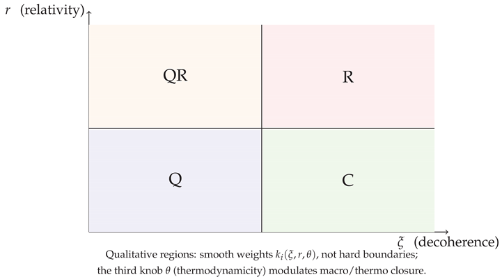
8. Qualitative Regime Figure

9. Conclusions

An operational meta-model for regime-aware prediction assembly has been presented. The framework combines (i) a shared observable space, (ii) soft loss-based weighting with regularization and complexity control, (iii) physics-facing regime priors via calibrated knobs, and (iv) a diagnostic for persistent out-of-catalog mismatch. The proposal is deliberately incremental: it is intended as a practical decision layer on top of existing mechanistic models, with clear calibration and validation hooks.

References

- Box, G. E. P.; Draper, N. R. Empirical Model-Building and Response Surfaces; John Wiley & Sons, 1987. [Google Scholar]
- Akaike, H. A new look at the statistical model identification . IEEE Transactions on Automatic Control 1974, 19(6), 716–723. [Google Scholar] [CrossRef]
- Schwarz, G. Estimating the dimension of a model . Annals of Statistics 1978, 6(2), 461–464. [Google Scholar] [CrossRef]
- Rissanen, J. Modeling by shortest data description . Automatica 1978, 14(5), 465–471. [Google Scholar] [CrossRef]
- Hoeting, J. A.; Madigan, D.; Raftery, A. E.; Volinsky, C. T. Bayesian model averaging: A tutorial . Statistical Science 1999, 14(4), 382–417. [Google Scholar] [CrossRef]
- Catoni, O. PAC-Bayesian Supervised Classification: The Thermodynamics of Statistical Learning, IMS Lecture Notes–Monograph Series, 2007.
- Amari, S.-I. Information Geometry and Its Applications; Springer, 2016. [Google Scholar]
- Jacobs, R. A.; Jordan, M. I.; Nowlan, S. J.; Hinton, G. E. Adaptive mixtures of local experts . Neural Computation 1991, 3(1), 79–87. [Google Scholar] [CrossRef] [PubMed]
- Zurek, W. H. Decoherence, einselection, and the quantum origins of the classical. Rev. Mod. Phys. 2003, 75, 715–775. [Google Scholar] [CrossRef]
- Breuer, H.-P.; Petruccione, F. The Theory of Open Quantum Systems; Oxford University Press, 2002. [Google Scholar]
- Jaynes, E. T. Information Theory and Statistical Mechanics. Phys. Rev. 1957, 106, 620–630. [Google Scholar] [CrossRef]
- Zwanzig, R. Nonequilibrium Statistical Mechanics; Oxford University Press, 2001. [Google Scholar]
Disclaimer/Publisher’s Note: The statements, opinions and data contained in all publications are solely those of the individual author(s) and contributor(s) and not of MDPI and/or the editor(s). MDPI and/or the editor(s) disclaim responsibility for any injury to people or property resulting from any ideas, methods, instructions or products referred to in the content. |
© 2026 by the authors. Licensee MDPI, Basel, Switzerland. This article is an open access article distributed under the terms and conditions of the Creative Commons Attribution (CC BY) license (http://creativecommons.org/licenses/by/4.0/).
Copyright: This open access article is published under a Creative Commons CC BY 4.0 license, which permit the free download, distribution, and reuse, provided that the author and preprint are cited in any reuse.