
Submitted:
26 February 2026
Posted:
28 February 2026
You are already at the latest version
Abstract
Forecasting stock prices, market trends, and associated emotions remains a complex challenge due to the market's inherent volatility, nonlinearity, susceptibility to factors such as news events, and the limited availability of financial data. Stock prices are noisy, unpredictable, and sensitive to investor sentiment \cite{ko2021, dahal2023, kumarsh2025}. To account for this, this study considers three models that effectively capture both the spatial relationships (similar sector stocks) between stocks and the temporal trends in their price movements, thereby addressing limitations in traditional forecasting methods. Specifically, we consider semiconductor stocks, which are known for their high volatility and strong correlation to technological advancements. The proposed models include Long Short-Term Memory (LSTM) and Gated Recurrent Unit (GRU) neural networks, a GNN-based architecture, and a Spatio-Temporal Graph Neural Network (ST-GNN). These models are trained, tested, and validated on datasets that combine historical data with sentiment insights from financial news sources. It utilizes a GRU-based temporal module to improve recognition of evolving market patterns. We demonstrate our model's ability to adapt to dynamic financial environments and predict whether a stock closes at a higher or lower price than at the trading day open.
Keywords:
sentiment analysis
; stock forecasting
; classification
; RNN
; sequential model
; ST-GNN
; performance analysis
1. Introduction
Predicting stock market movements is an inherently challenging task due to the market’s complex, volatile, and non-linear nature [16]. Numerous factors, including economic conditions, company performance, geopolitical events, and investor psychology, influence stock prices, make accurate forecasting difficult for investors and financial analysts aiming to optimize returns and mitigate risks [23,24]. Traditional forecasting methods, such as fundamental and technical analysis, often prove insufficient, especially for short-term predictions due to their limitations in capturing the market’s intricate dynamics and nonlinear relationships [21]. Theories like the Efficient Market Hypothesis and Random Walk Theory further suggest that historical data alone may be inadequate, as stock prices can be influenced by unpredictable news and external factors [18].
Traditional models, such as ARIMA (Autoregressive Integrated Moving Average) or statistical time-series approaches, often struggle to capture the intricate web of relationships that influence stock prices, especially in response to investor sentiment, macroeconomic changes, and external shocks [26]. Machine learning and deep learning , which are the basis for the models explored in this study, are more sophisticated approaches for capturing complex patterns in financial data. Conventional machine learning methods, however, have struggled with incorporating structural information across related assets and adapting effectively to evolving interdependencies between companies, sectors, and economic indicators.
In recent years, researchers have increasingly turned to alternative data sources, particularly textual data from news feeds and social media to gauge investor sentiment and its potential influence on market movements [19]. Sentiment analysis, which involves extracting opinions or emotions from text, has emerged as a complementary signal for forecasting stock behavior [17]. This rationale is rooted in behavioral finance, which posits that public mood and sentiment can influence investment decisions, thereby affecting stock prices [16]. Early studies provided evidence that information from internet message boards and news articles could predict market volatility and price movements, respectively.
The applications of neural network-based methods, including Recurrent Neural Networks (RNNs) and Graph Neural Networks (GNNs), for stock prediction often rely on historical price data and derived technical indicators, such as Close, Volume, RSI, and MACD. While these capture market momentum and trends, they may not fully encompass the influence of investor sentiment, which is driven by news, economic conditions, and broader market psychology. RNNs, specifically Long Short-Term Memory (LSTM) and Gated Recurrent Unit (GRU) networks, have gained prominence for time series forecasting. Their architectures are designed to learn long-range dependencies that are often missed by simpler models, making them well-suited for modeling sequential data, such as stock prices. The LSTM and GRU networks show significant success in learning long-range dependencies in sequential data [23,27,28]. The GNNs are also a robust framework capable of modeling relationships between financial entities as graph data structures. These models generally treat stock prices as isolated time series and overlook inter-stock relationships and qualitative data such as news sentiments. Despite advancements in GNN, many existing models fall short in handling both spatial and temporal dependencies effectively [15]. Some approaches fail to adequately integrate sentiment data, while others struggle to adapt to evolving market behaviors [14].
Additionally, by combining traditional stock data with financial sentiment extracted from news headlines and descriptions, the program seeks to improve forecast accuracy. The effectiveness of stock price prediction can be enhanced by combining sentiment analysis with neural network-based models [19]. The sentiment analysis provides a means to quantify this dimension. This study aims to evaluate whether augmenting three models (LSTM, GRU, and ST-GNN) with general sentiment scores enhances predictive accuracy for daily stock closing prices compared to models using only conventional technical indicators. It also compares the performance metrics of these models under both sentiment-inclusive and sentiment-exclusive conditions.
Sentiment plays a role in shaping both short and long-term stock movements. Influenced by financial news, market community, and public discourse, investors will determine whether to invest or not. To extract financial sentiment for incorporation into our models, a transformer-based model, Bidirectional Encoder Representations from Transformers (BERT), and its financial variant, FinBERT, are utilized to calculate sentiment scores [31,32]. FinBERT enables more sophisticated extraction of sentiment signals from financial texts. When integrated with numerical data, sentiment analysis can improve the interpretability and performance of financial forecasting systems. Furthermore, the sentiment score is generated for key business areas, including artificial intelligence, cloud computing, e-commerce, logistics, and finance. To account for short-term memory effects, these scores are compared to historical stock data that has been cleansed, normalized, and enhanced with time-based features and lag variables [4,7,8,32,33].
The model’s capacity to identify connections between sentiment influenced by news and short-term price swings, supported by the ability to combine Natural Language Processing (NLP), BERT, and FinBERT with graph-based deep learning, enables this capability. In this study, we demonstrate how structured financial data and unstructured textual and sentiment data can be combined to improve the responsiveness of stock price forecasting and context awareness. Stock forecasting is further improved by incorporating a sentiment score into predictive mode and comparing the performance metrics of RNNs’ LSTM and GRU architectures, as well as GNNs’ ST-GNN. The ST-GNN model integrates technical indicators, historical price data, and sentiment features extracted via FinBERT to enhance prediction accuracy in the stock market, with a specific focus on the e-commerce sector. Additionally, the LSTM serves as a baseline model to assess the impact of general market sentiment on RMSE, MAE, and directional accuracy. Whereas ST-GNN is used for topic-specific sentiment signals, such as AI, logistics, and cloud computing, it is combined with graph-based temporal data to model sector-wide dependencies. Finally, these methods ensure the consistency of sentiment data’s impact across multiple stocks within the semiconductor sector and across three forecasting models. A principal aim of this work is to demonstrate the practical value of deploying hybrid LSTM and ST-GNN models in real-world trading and policy contexts [23].
This paper is organized as follows. Section 1 explains the fundamental reasons for adding sentiments and available approaches for forecasting stock prices. In Section 2 we discuss model results with and without sentiment integration in stock price datasets. Section 3 presents the datasets and their integration, as well as the statistical significance related to this study, as outlined in the Materials and Methods. The corresponding predicted prices, findings, performance analysis, and their significance are presented in the Results and Discussion Section 4. Finally, Section 5 summarizes the findings of the experiments.
2. Background
As financial markets grow increasingly complex and interconnected, researchers have begun turning to neural network-based deep learning models, including GNNs, to better model and predict stock price movements. The Autoregressive Integrated Moving Average (ARIMA), one of the most well-known conventional models, uses linear regression on lagged values and forecast errors to explain time-dependent structures [26]. However, ARIMA and similar statistical methods are often insufficient in highly volatile or nonlinear environments and are particularly limited when incorporating unstructured external information such as news or social media sentiment.
To address the limitations of ARIMA, Recurrent Neural Networks (RNN), more specifically Long Short-Term Memory (LSTM) networks, were introduced to manage long-term dependencies and sequential patterns in stock data [27]. LSTMs demonstrated superior performance on stock data ; however, LSTMs struggle to process data in non-Euclidean formats, such as graphs that show the interactions between sentiment, price dependence, and time [28]. A GNN framework improves this shortcoming by integrating multi-source heterogeneous data. We introduce a method of embedding these diverse inputs into GNN graph-based representations and show its ability to predict stock volatility and uncovered patterns that conventional models typically miss [13].
In [5], a Hybrid and Temporal Graph Neural Network (HT-GNN) model was discussed that leverages supply chain networks and time-dependent embeddings to capture the influence of related companies on a target firm’s stock performance. The integration of firm-level partnerships beyond immediate ties proved especially effective, highlighting that interconnected economic relationships often provide predictive insights into stock performance. Building on the strengths of these approaches, [12] developed a Temporal and Heterogeneous Graph Neural Network (TH-GNN) that models stock price fluctuations using dynamic and heterogeneous relational data. By combining temporal encoders with graph-based attention mechanisms, their method improves both short-term and long-term prediction accuracy. The TH-GNN’s ability to dynamically adjust node relationships in response to changing market conditions demonstrated improved robustness in volatile financial environments.
To overcome these structural limitations, researchers have adopted Graph Neural Networks (GNNs), which extend deep learning methods to graph-structured data by modeling relationships between entities. [29,35] introduced Graph Convolutional Networks (GCNs), which extend convolution operations to nodes and their neighbors in a graph. This generalizes convolution operations to graph topologies, enabling the aggregation of information across connected nodes. These models have been helpful in domains such as social networks, traffic systems, and finance [34].
The integration of temporal dynamics led to the emergence of Spatial-Temporal Graph Neural Networks (ST-GNNs), which model spatial and temporal dependencies. In transportation systems, where a traffic node’s future state is dependent on nearby nodes and previous time steps, ST-GNNs have been successfully implemented [30]. This makes ST-GNNs uniquely suited to capture evolving patterns in financial networks, outperforming traditional sequence models in various forecasting tasks.
Another essential component of financial modeling is sentiment analysis, which quantifies investor sentiment based on unstructured textual data, such as news headlines, reports, and social media posts. While early methods relied on lexicon-based systems like VADAR and TextBlob, they lack contextual depth and failed to capture domain-specific nuance. The introduction of pre-trained transformer models, such as BERT, has significantly enhanced the capabilities of NLP. When it comes to detecting subtle sentiment in news headlines and analyst reports, FinBERT, a domain-specific version of BERT optimized for financial texts, was used [31,32] discovered that FinBERT significantly outperformed CNN-based or LSTM-based models in their ability to categorize financial sentiment, especially when it came to predicting stock returns based on event-driven news.
Combining FinBERT’s sentiment features with ST-GNN architectures creates a hybrid framework that integrates both quantitative and qualitative signals. This combination could enhance predictive performance, particularly in volatile markets where behavioral factors are highly influential. Thus, this study builds upon these prior advancements by proposing an ST-GNN architecture that is used for stock price prediction in the semiconductor and e-commerce sectors. This model will incorporate dynamic edge types, temporal encoders, and topic-specific sentiment features extracted via FinBERT (sentiment analysis relevant to firms such as Amazon, focusing on areas like AI, logistics, and cloud computing). Inspired by HT-GNN’s use of inter-firm dynamics and MSub-GNN’s multi-source fusion, the goal is to improve forecasting stability and contextual awareness.
The integration of sentiment analysis with deep learning (DL) methods has become a prominent approach to enhance stock price forecasting accuracy [25]. Deep learning models, particularly RNNs and their variants such as LSTM and GRU, are well-suited for analyzing sequential time-series data, including stock prices and textual sentiment [20]. The RNN’s LSTM architecture is highly suitable for modeling sequential data like financial time series due to its ability to capture long-term temporal dependencies while addressing the vanishing gradient problem typical of traditional RNNs [18,21]. LSTMs employ a gating mechanism—input, forget, and output gates—to selectively retain relevant past information, making them particularly effective for predicting stock price movements from historical price data combined with sentiment analysis [19]. Empirical studies consistently illustrate that LSTM-based models outperform conventional statistical models by integrating sentiment metrics, thereby capturing market reactions to evolving news or events with greater precision [17].
The RNN’s GRU architecture is a simpler version of LSTMs, offering a simplified yet efficient alternative to LSTM networks. In [23], GRUs merge the LSTMs’ forget and input gates into a single update gate, while maintaining a reset gate, thereby reducing computational complexity while still effectively managing sequence prediction tasks [20]. The GRUs have significant performance advantages, particularly in noisy or volatile data environments, which are typical of financial markets. For instance, the GRUvader model demonstrated superior stock prediction capabilities by effectively integrating sentiment indicators, thereby affirming the robustness and efficiency of GRUs in handling complex financial sequential data [22]. Despite these advances, several issues remain open. Model transparency remains limited; stakeholders struggle to interpret hidden-state dynamics when forecasts deviate from intuition. Additionally, models’ performance varies with data provenance—such as lexicon-based scores, tweet moods, or authoritative-site news—and with temporal alignment between sentiment shocks and price reactions. It has been observed that comparative studies under identical conditions are scarce, making it hard to disentangle architecture effects from data and tuning choices [4,7,8,20,22].
Lastly, these models are designed to consider adaptive learning rates and dynamic lookback windows, allowing for responsiveness in high-volatility conditions. By modeling the market as a temporally evolving RNN and graph enriched with sentiment signals, this study marks a step forward in integrating GNN-based strategies into real-world financial forecasting.
3. Materials and Methods
The dataset description and methods are described in this section.
3.1. Datasets Description
Historical stock market data and financial news articles are the two primary sources of information. The stock market data provides key financial indicators necessary for time-series analysis, while financial news articles contribute to external market sentiment, forming a comprehensive dataset for RNN’s LSTM and GRU architectures, as well as GNN model-based stock forecasting.
3.1.1. Stock Market Data Collection
Stock market data retrieved from Yahoo Finance using the yfinance Python library [7,8,9]. The dataset comprises historical stock prices and fundamental financial indicators for a select group of semiconductor companies. The companies analyzed include Advanced Micro Devices (AMD), ASML Holding (ASML), Broadcom Inc. (AVG), Intel (INTC), Marvell Technology Inc. (MRVL), Micron Technology Inc. (MU), NVIDIA Corp, (NVDA), Qualcomm (QCOM), Taiwan Semiconductor Manufacturing Company (TSMC), Texas Instruments (TXN) [4,7,8].
The dataset captures essential financial attributes for each stock, including the closing price, which represents the final stock price at the end of each trading day, and trading volume, indicating the number of shares traded. Additionally, several technical indicators, such as the Relative Strength Index (RSI) and Moving Average Convergence Divergence (MACD), are computed to enhance the analysis of stock price movements. Also, fundamental metrics such as the Price-to-Earnings Ratio (P/E Ratio) and Earnings Per Share (EPS) are incorporated. Collectively, these attributes provide a robust basis for predicting future stock movements by capturing various dimensions of market behavior.
The datasets’ structure is consistent across all stocks. To complement numerical stock data with qualitative insights, financial news articles about each stock were gathered from an external API provided by RapidAPI [10]. The financial news dataset consists of multiple attributes: Stock Symbol, News Title, Publication Source, Date of Publication, and News Article URL. The articles were retrieved from multiple sources, including Simply Wall St, Coin Telegraph, The Hindu, The Register, and Kadena Air Base, ensuring coverage from financial, mainstream, and industry-specific media. Each article was stored in a structured format, facilitating further preprocessing for sentiment analysis.
3.1.2. Data Distribution and Exploratory Data Analysis
The data acquisition and preprocessing have been performed using Python scripts, which automate the collection, cleaning, wrangling, and structuring of stock and news data. The retrieval of stock price and financial indicator data using the Yahoo Finance API calculates key technical indicators, including RSI, MACD, P/E Ratio, and EPS. After obtaining these metrics, dataset consistency has been ensured across different stock tickers and financial attributes. This structured format facilitates further analysis and model training, allowing for seamless integration with deep learning models. Furthermore, another Python script collects real-time financial news articles using an API-based approach. It begins by querying a financial news API to retrieve headlines and summaries related to selected semiconductor companies. This ensures that the dataset includes relevant market developments that may influence stock movements. Once the articles are retrieved, they are structured for each data object, which consists of the news title, source, publication date, and URL. This structured format streamlines the sentiment analysis process, enabling efficient extraction of sentiment-based insights from financial news.
By integrating both stock market and news sentiment datasets, the GNN model leverages historical financial data alongside sentiment-driven insights to enhance the accuracy of stock price movement predictions. Evaluating the overall market sentiment and sentiment related to specific financial topics, a pre-trained FinBERT model is used for sentiment classification, supplemented by TextBlob for linguistic processing and spaCy for named entity recognition (NER) [32,33]. Thereafter, the collected data from financial news articles are processed into an appropriate structure with dimensions: stock, title, description, data, and URL.
The data distribution and descriptive statistical values of normalized stock prices for AMD, ASML, AVGO, INTC, MRVL, MU, NVDA, QCOM, TSM, and TXN over a specified period are illustrated in Figure 1. Also, Figure 1 (b) demonstrates that there are no potential outliers. Stocks like NVDA and TXN exhibit a broader price range, indicating greater variability in their trading behavior, while others, such as MRVL and MU, show more concentrated distributions with fewer extreme deviations.
3.2. Data Preprocessing
The dataset is preprocessed, where the ’Date’ column in the stock dataset was converted to a datetime data type, and the entire dataset was sorted chronologically by ’Stock’ ticker and then by ’Date’ to ensure proper temporal ordering. The ’General Sentiment Score’ was appended to the primary stock dataset. Missing sentiment values in this dataset were filled in using a backward-fill technique, followed by a forward-fill technique to handle initial NaNs. Moreover, two primary feature variants are constructed for each stock. The first, termed ’no_sentiment’, included traditional technical indicators: ’Close’ price, ’Volume’, ’Relative Strength Index’ (RSI), and ’Moving Average Convergence Divergence’ (MACD). Any rows containing NaN values for these core features were dropped. The second variant, labeled ’forward_fill’ (also referred to as ’with_sentiment’), incorporated these same technical indicators along with the newly derived ’General Sentiment Score’. This approach allowed for a direct comparison of model performance with and without the inclusion of sentiment data. A minimum data length, defined as the lookback window plus 20 data points, is enforced. Stocks or variants that do not meet this threshold are excluded from the analysis to ensure sufficient data for robust model training. All the available data passed through this process.
3.3. Sentiment Score and Sentiment Analysis using FinBERT
The FinBERT model is used to determine if a positive sentiment score indicates bullish sentiment (optimism in the market), a negative sentiment score indicates bearish sentiment (concerns or pessimism), and a sentiment score near zero suggests neutral sentiment [32,33].
The sentiment analysis workflow begins with data loading and preprocessing, where financial news articles are retrieved from the dataset. These articles are then parsed, and any irrelevant or missing data is filtered out to ensure the quality and reliability of the dataset. Following preprocessing, a general sentiment is computed. Each article’s headline and description are combined into a single text input to capture the overall sentiment expressed in the news. The text is then tokenized and vectorized using FinBERT’s tokenizer, a language model designed explicitly for financial text analysis. Once processed, a sentiment score is computed for each article, quantifying whether the news sentiment is positive, negative, or neutral. In addition to general sentiment classification, the script conducts topic-specific sentiment extraction to analyze sentiment at a more granular level.
Finally, the sentiment scores are aggregated daily for each stock to facilitate time-series analysis. The general sentiment scores are stored in *.csv file, which has three dimensions – Date, Stock Name, and General Sentiment Score. Whereas the topic-specific sentiment scores are recorded in another *.csv file into three dimensions – Date, Stock Name, and Topic Sentiment Score. These structured datasets offer valuable insights into sentiment, which can be integrated into predictive models to enhance the accuracy of stock price forecasting. Moreover, after running the sentiment analysis pipeline for 372 days on 10 stocks, the average general sentiment score is 0.534. On the other hand, for six topics and 22,320 total topic-stock-day combinations, the score of the topic-based sentiment analysis is 0.007.
Afterwards, the extracted sentiment scores are then integrated into the Graph Neural Network (GNN) model, where they serve as external features to improve predictive accuracy. To summarize, the sentiment analysis framework effectively quantifies the emotional tone of financial news articles, offering valuable insights into investor sentiment.
3.4. RNN’s LSTM, and GRU
Once the feature sets are preprocessed, the data for each stock variant is partitioned into training and testing sets. The data was split chronologically, with the initial 80% of the data designated for training and the remaining 20% for testing. This chronological split was decided to prevent data leakage from the future into the training process, thereby ensuring a more realistic evaluation of the models’ predictive capabilities.
Prior to model training, all input features were normalized using a ‘MinMaxScaler’ from the ‘sklearn.preprocessing’ library. This scaler transforms the features to a range between 0 and 1, which helps stabilize and speed up the training process for neural networks. The MinMaxScaler was fitted only on the training data for each feature set. The scaler, once fitted, was then used to transform both the training and the test sets, ensuring that no information from the test set influenced the scaling parameters of the training data. The ’Close’ price was designated as the target variable for prediction.
To prepare the data for the sequential LSTM and GRU models, a helper function, ‘create_sequences’, was created. This function transformed the scaled time-series data into input sequences (X) and corresponding target values (y). For each sequence, X consisted of the feature values from the previous ‘LOOKBACK_WINDOW’ (60) time steps, and y was the scaled ’Close’ price of the subsequent day. This sliding window approach enables the models to learn temporal patterns from past observations, thereby predicting future values. If, after processing, either the training or testing sequence arrays were empty, that particular stock variant was skipped for the modeling phase as a precaution.
For a fair and direct comparison of LSTM and GRU capabilities, both model architectures were constructed with an identical number of layers and units. Each model comprised two recurrent layers: the first LSTM/GRU layer had 100 units and was configured to return the complete hidden-state sequence (’return_sequences=True’). This was followed by a Dropout layer with a rate of 0.20 to mitigate overfitting. The second LSTM/GRU layer had 50 units and returned only the final hidden state (’return_sequences=False’). This was also followed by a Dropout layer with a 0.20 rate. Subsequently, a Dense layer with 25 neurons and ReLU activation function was added, followed by a final Dense output layer with a single linear neuron to produce the next day’s closing price forecast. The random seed was fixed for TensorFlow, NumPy, and Python’s random module to ensure reproducibility of results.
The models were trained using the Adam optimizer with a learning rate of 0.001. Mean Squared Error (MSE) was employed as the loss function to quantify the difference between the predicted and actual stock prices during training. Training was conducted with a batch size of 32 for a maximum of 150 epochs. To prevent overfitting and reduce training time, an ’EarlyStopping’ callback mechanism was implemented. This mechanism monitored the validation loss (’val_loss’) on the test set during training and halted the training process if the validation loss did not improve for a specified ’EARLY_STOPPING_PATIENCE’ of 10 epochs, restoring the model weights from the epoch with the best validation loss.
The performance of the trained LSTM and GRU models for each stock and feature variant was rigorously evaluated using three standard metrics: Root Mean Squared Error (RMSE), Mean Absolute Error (MAE), and Directional Accuracy. RMSE and MAE measure the magnitude of prediction errors, with lower values indicating better accuracy. Directional Accuracy assesses the models’ ability to correctly predict the direction (up or down) of stock price movements relative to the previous day’s actual closing price, providing a measure of practical usefulness for trading decisions. Predictions were first made on the scaled test data and then inverse-transformed back to the original price scale using the previously fitted ’MinMaxScaler’, ensuring that the evaluation was performed in the context of actual price values. The training history, including loss and validation loss per epoch, as well as the actual versus predicted prices for the test set, was saved for further analysis.
3.5. Additional Data Preprocessing for ST-GNN
The ST-GNN requires an integrated dataset, which combines both financial metrics and sentiment analysis scores. It ensures data consistency, handles missing values, and selects meaningful features that improve the model’s predictive performance. Furthermore, the data is then normalized and structured to ensure compatibility with the ST-GNN model, thereby enhancing its ability to recognize complex patterns. Preprocessed data consists of twenty dimensions – Date, AMD_Close, AMD_Volume, AMD_PE_RA, AMD_EPS_, AMD_MACD_, AMD_RSI_, ASML_Close, ASML_Volume, ASML_PE_RA_, ASML_EPS_, ASML_MACD_, ASML_RSI_, AVGO_Close, AVGO_Volume, AVGO_PE_RA_, AVGO_EPS_, AVGO_MACD_, AVGO_RSI_, INTC_Close, INTC_Volume, etc.
Financial time series data often presents missing values due to non-trading days or incomplete sentiment information. To address this, forward-fill imputation is employed, ensuring the continuity of stock price trends. After handling missing values, Min-Max normalization is applied to stock prices, trading volumes, and sentiment scores. Normalization is crucial for ST-GNN models, as it scales all input features to a uniform range (0 to 1), thereby preventing numerical instability during the training phase [34].
To determine similarity among dimensions, a correlation analysis is conducted to assess the correlation values among features and the stock closing prices. Upon evaluation, it was determined that all features exhibit meaningful contributions to the dataset. Consequently, no features were excluded. This comprehensive inclusion aims to leverage the robustness of STGNNs, which are adept at processing multifaceted information to capture intricate spatial-temporal patterns. Retaining a diverse set of features can enhance the model’s resilience and predictive accuracy. ST-GNN models are particularly well-suited for this type of data, as they can effectively model complex relationships between stocks and market sentiment over time [2,23,34].
The final preprocessing step involves transforming the dataset into a format amenable to graph-based learning. This preprocessing framework equips the stock market dataset for ST-GNN application by integrating financial indicators with sentiment analyses, conducting correlation-based feature assessments, imputing missing values, and normalizing data to ensure model stability. By structuring the data in a graph-compatible format, this approach enhances the ST-GNN’s capacity to discern complex interdependencies between stocks and external market sentiments, thereby improving the accuracy of stock price forecasts.
3.6. Graph Construction for ST-GNN
A stock relationship graph is shown in Figure 2, where each stock is a node, and edges are formed based on multiple financial and sentiment-based correlations. This graph is then used to train an ST-GNN to model both spatial dependencies and temporal trends in stock market data. Subsequently, by integrating both technical indicators and sentiment-based metrics, the graph captures fundamental stock behaviors and shifts in investor sentiment. Additionally, general sentiment scores and topic sentiment scores measure the impact of news articles on investor perception [3]. Each stock node is assigned these features, ensuring a comprehensive representation of financial and sentiment-related influences on stock performance.
Edges between nodes represent relationships between stocks based on multiple financial attributes. To construct meaningful connections, the model calculates correlation matrices for different stock attributes, including closing price, trading volume, RSI, and MACD. These edges provide structural relationships that enhance the ST-GNN’s ability to detect patterns in stock behavior beyond independent price movements [1]. Furthermore, beyond price and volume correlations, the model incorporates sentiment-driven relationships. The two primary sentiment-based edges formed are General Sentiment Correlation Edges and Topic Sentiment Correlation Edges. By including sentiment-based dependencies, the model extends beyond traditional price-based stock connections, incorporating a layer of qualitative market influence.
Once the graph is constructed, it is converted into a format suitable for PyTorch Geometric, a framework optimized for GNN-based learning [11]. The edge list, containing financial metric-based and sentiment-based relationships, as well as the node feature matrix, is stored for further use. Each edge is also assigned a weight and type, which is stored separately. After graph construction, key statistics are computed to validate the graph’s structure and ensure that it accurately reflects the relationships between the stock market. The model reports the total number of nodes, representing unique stocks in the dataset. It also reports the total number of edges, quantifying price-based and sentiment-based connections.
The enhanced graph-based representation of stock market data provides a robust foundation for training ST-GNN models, integrating technical indicators, fundamental metrics, and sentiment-based relationships. By leveraging multiple financial correlations and market sentiment trends, this approach enables a comprehensive understanding of stock dependencies, ultimately improving stock trend forecasting accuracy [1,3]. The inclusion of multi-attribute edges ensures that the model captures both quantitative price movements and qualitative sentiment-driven influences, aligning with recent advances in graph-based financial modeling. Additionally, the Enhanced Stock Relationship Graph offers a structural view of the relationships between semiconductor stocks, based on multiple financial indicators. The graph consists of 10 stocks and 43 edges, slightly lower than the previous estimate, indicating a well-connected but not fully dense network. The graph highlights distinct clusters formed by different relationship types, such as their positions in the graph. Price trends and market sentiment remain the dominant factors shaping stock relationships, while technical indicators and volume have a secondary influence. The most highly connected stocks, such as AMD and NVDA, serve as central nodes within the network, while TSM and ASML maintain strong sentiment-based connections. The graph confirms that price and sentiment should be prioritized when analyzing stock relationships, as they provide the strongest signals for predicting market movements and building stock relationship models.
3.7. Building the ST-GNN Model
The ST-GNN model is designed to predict stock prices by combining spatial relationships between stocks with temporal dependencies in their financial data. The model’s first component is the Graph Convolutional Network Layer (GCN), which captures spatial relationships between stocks. In this architecture, each stock is represented as a node in a graph, while edges encode relationships such as price correlations, sentiment similarities, and technical indicator correlations. In this implementation, the model extends traditional GCN layers by introducing support for multiple edge types. This method follows the principles described in Labonne’s work on multi-relational graphs [2,6].
To capture time-dependent trends in stock price data, the model incorporates a Temporal Module. This module processes the evolving financial data, producing a hidden state that encodes the temporal dependencies. The model builds node features by combining various financial indicators, including the closing price, which represents the final stock price at market close, and trading volume, which indicates the number of shares traded in each period.
The ST-GNN model integrates nodes and edges through a structured workflow. First, nodes are constructed for individual stocks with enriched financial indicators, while edges are defined using correlations and sentiment-based connections. The graph convolutional layers apply distinct convolution operations for each edge type and combine their outputs using an attention mechanism that emphasizes key relationships. The temporal module processes sequential stock data, enabling the model to capture evolving trends in financial indicators and market sentiment. Finally, the model’s prediction layer generates future stock price forecasts over a specified time horizon.
The model is trained using backpropagation with a loss function designed to minimize forecasting errors. To improve generalization and prevent overfitting, the model applies dropout regularization during training. This ensures that the model can effectively adapt to unseen data. By combining graph convolutional layers with recurrent temporal layers, the model efficiently extracts meaningful patterns in both financial indicators and market sentiment [2,6].
3.8. ST-GNN Model Training
The training and evaluation of the ST-GNN model involves several key steps designed to ensure the model achieves optimal performance. The training process begins by iterating through the training dataset, adjusting the model’s internal weights and other hyperparameters to minimize prediction errors. Upon completion, the trained model is saved, ensuring that it can be reused without requiring retraining. The training process can accept custom hyperparameters such as batch size, learning rate, and the number of epochs. For example, a batch size of 32, a learning rate of 0.001, and 100 epochs are used, allowing users to adjust the model’s training behavior based on the dataset size, computational resources, and desired accuracy.
Once the model is trained and predictions are made. The trained ST-GNN model applies it to predict future stock prices. The predicted results are saved in the specified output directory, making it easier for analysts to review and interpret the model’s forecasts. Also, users can apply the model directly to new financial data without requiring additional training steps. This prediction phase plays a crucial role in translating the model’s learning into actionable insights for financial forecasting.
To assess the model’s accuracy and effectiveness, the model compares the ST-GNN model’s predictions with those from baseline models to measure improvements in predictive accuracy. The evaluation step generates detailed performance metrics and visualizations, providing a clear understanding of the model’s strengths and weaknesses. The outputs highlight key metrics, including mean squared error (MSE), mean absolute error (MAE), and R-squared values. These insights are essential for validating the model’s reliability and ensuring that its predictions are both accurate and consistent across various financial scenarios.
Moreover, initially, the model was constructed with two GNN layers, one temporal layer using a GRU cell, and hidden dimensions set to 48. The model is trained with a batch size of 8 for 60 epochs, using a learning rate of 0.001 with step decay adjustments. Early stopping occurred at epoch 29 with the best validation loss observed at epoch 23, recorded at 0.0587. Despite achieving some predictive accuracy, the model displayed signs of instability and potential overfitting, indicating the need for refinement. To address these issues, several adjustments were introduced, starting with the reduction of model complexity. By reducing the number of hidden dimensions from 48 to 32, the model became less prone to overfitting while maintaining its original shallow architecture. Training stability was also improved by lowering the learning rate to 0.0005 and increasing the batch size from 8 to 16, which contributed to more stable gradients. Additionally, extending the number of training epochs to 100 allowed the model more time to converge on optimal weights. These changes collectively improved the model’s generalization capabilities, making it more adaptable to unseen data.
The impact of these refinements is reflected in the final training results. The model completed training in 247 epochs, achieving a training loss of 0.0049 and a validation loss of 0.0032, which represents a remarkable 94.55% improvement from the initial validation loss of 0.0587. Training stability improved significantly, with reduced oscillations in the loss curve, demonstrating more consistent convergence behavior. The improved generalization capabilities ensured that the model maintained an effective balance between training and validation performance, reducing the risk of overfitting. Figure 3, Training Progress Comparison, illustrates this enhanced stability and convergence, showcasing smoother progression with fewer fluctuations throughout the training process. This visual evidence reinforces the effectiveness of the carefully tuned architecture, training dynamics, and optimization strategies in achieving improved model performance.
Figure 3 illustrates the progression of both training and validation losses throughout model development. The initial training run, represented by blue lines, displayed a stepped learning rate pattern with sharp drops at scheduled learning rate reductions. In contrast, the improved model, represented by the red lines, exhibited a smoother and more stable decline (convergence) in loss values due to the enhanced training strategies. The visual comparison highlights how adjustments to learning rate scheduling, model architecture, and training patience contributed to more stable and effective learning dynamics.
3.9. Evaluating ST-GNN Model
The performance analysis of the ST-GNN model reveals notable differences between its performance on the validation set and the test set, with valuable insights for future improvements and risk management. On the validation set, which represents the middle 15% of the data, the model achieved strong predictive accuracy with a mean squared error (MSE) of 0.0031, a root mean squared error (RMSE) of 0.056, and an R² score of 0.804. These metrics indicate that the model was highly effective during training, suggesting that the chosen architecture and hyperparameter tuning were well-optimized. However, on the test set, which represents the most recent 15% of the data, the model’s performance declined with an MSE of 0.0063, an RMSE of 0.079, and an R² score of 0.634. While still demonstrating useful predictive power, the increased error rates highlight the challenges of applying the model to unseen, real-world data.
The performance gap between the validation and test sets can be attributed to several factors. Since the test set represents more recent data, changes in market conditions or emerging trends may have impacted the model’s effectiveness. Financial markets are inherently dynamic, and factors such as economic developments or shifts in investor behavior could introduce data drift, altering the relationship between features and the target variable. Despite these challenges, the model’s improved generalization strategies helped retain a meaningful degree of accuracy. By extending the lookback window to 30 days, adjusting dropout rates, and adopting the AdamW optimizer, the model achieved greater stability and resilience. The consistent contribution of sentiment analysis also played a significant role in improving predictive power across both the validation and test sets.
In earlier training attempts, the model’s learning curve displayed sharp oscillations, with abrupt shifts at learning rate adjustments. In contrast, the refined model’s learning curve shows smoother, more controlled progression, reflecting improved stability. While the test set exhibits higher error rates than the validation set, the model’s ability to produce actionable predictions with appropriate risk adjustments makes it suitable for various trading strategies.
Figure 4 illustrates the actual stock prices against the predicted prices, revealing the model’s core predictive power. Each point on the plot represents a prediction, with the x-axis indicating the actual price and the y-axis showing the model’s prediction. The overall pattern suggests that, although the model isn’t perfect, it consistently captures the general price movements. This visualization helps us understand that the model is particularly good at predicting price ranges but may occasionally miss extreme price movements, which is typical for financial prediction models.
Figure 5 illustrates the factors that have the most decisive influence on the model’s predictions. At the top of the rankings, we see EPS (Earnings Per Share) and MACD (Moving Average Convergence Divergence) as the most influential features, followed closely by PE Ratio and RSI (Relative Strength Index). This ranking makes intuitive sense because EPS represents a company’s fundamental performance, while MACD captures technical market trends. Figure 5 also reveals that sentiment analysis features, while helpful, are not the dominant factors in the model’s decision-making process. This suggests that while market sentiment is valuable, traditional financial metrics still play a more crucial role in price prediction. The relatively balanced distribution of importance across different types of features (technical, fundamental, and sentimental) validates our approach of using a multi-factor model.
Figure 6 demonstrates how the model’s prediction accuracy changes as we try to forecast further into the future. The graph shows a clear upward trend in RMSE (Root Mean Square Error) as the forecast horizon increases from 1 to 7 days. This is expected because predicting stock prices becomes more challenging as time passes. The rate of increase in error is exciting - it’s steeper in the first few days and then begins to level off. This suggests that while the model is most accurate for short-term predictions (1-2 days), it still maintains reasonable accuracy for medium-term forecasts (3-5 days). The graph helps us understand that the model is best suited for short to medium-term trading strategies, with diminishing returns for longer-term predictions. This information is crucial for practical trading applications, as it enables traders to set realistic expectations for the model’s performance at various time horizons.
4. Results and Discussions
The performance of RNNs’ LSTM and GRU, and ST-GNN is discussed in Section 4.1 and Section 4.2, respectively.
4.1. RNNs’ LSTM, and GRU Results
The performance of the LSTM and GRU models is computed by applying the prepared time-series sequences derived from the technical indicators (’no_sentiment’ variant) and the combination of technical indicators and imputed sentiment scores (’forward_fill’ variant). The performance of the trained models is evaluated on the respective test sets using performance metrics - Root Mean Squared Error (RMSE), Mean Absolute Error (MAE), and Directional Accuracy (DA). The performance metrics values are listed in Table 1, and predictions are demonstrated in Figure 7.
The RNN models are impacted significantly by sentiment data. On average, incorporating the imputed ’General Sentiment Score’ (’forward_fill’ variant) did not improve performance compared to using only technical indicators (’no_sentiment’). For both LSTM and GRU architectures, the ’no_sentiment’ variants yielded lower average RMSE and MAE. Directional accuracy was also slightly higher on average for the ’no_sentiment’ GRU models, while it remained the same for LSTM regardless of sentiment inclusion. Whereas, comparing the two architectures, GRU models generally outperformed LSTM models in terms of average error metrics (RMSE and MAE) within this experimental setup. The GRU ’no_sentiment’ configuration achieved the lowest average errors overall. GRU models also showed slightly better average directional accuracy than LSTM models.
Moreover, the stock-specific variability w.r.to. variants. The average results favored the ’no_sentiment’ approach and the GRU architecture, with performance varying considerably across individual stocks. For instance, sentiment appeared beneficial for GRU on INTC (RMSE 0.91 versus 1.19), sentiment significantly hindered performance for both models on ASML (e.g., GRU RMSE 12.79 vs 23.27) and AVGO (e.g., GRU RMSE 16.46 vs 19.54), and for NVDA, LSTM with sentiment (’forward_fill’) has lower RMSE than LSTM without (5.44 vs 7.02), but GRU without sentiment (’no_sentiment’) performed better than GRU with sentiment (RMSE 5.17 vs 6.21). Finally, the number of model training epochs significantly affects. Models trained without sentiment data (’no_sentiment’) generally required more training epochs before meeting the early stopping criteria compared to their ’forward_fill’ counterparts (Average epochs LSTM: 24.4 vs 16.9; GRU: 31.0 vs 38.2)
The collective results suggest that, within the constraints of this study’s methodology, integrating general sentiment data via a simple backfill/forward-fill imputation strategy did not consistently enhance, and often slightly degraded, the predictive accuracy of standard LSTM and GRU models for daily stock closing prices compared to using only technical indicators.
The RNN model shows that a lack of consistent benefit from sentiment data could stem from the following factors:
- Data Quality and Relevance: The ’General Sentiment Score’ might lack the specificity required for individual stock prediction or suffer from a low signal-to-noise ratio, potentially incorporating irrelevant market chatter.
- Imputation Method: The backfill/forward-fill approach is a basic method for handling missing data. It might introduce artificial stability or propagate stale sentiment values, potentially providing misleading signals to the models, especially if sentiment changes rapidly. More sophisticated imputation techniques or methods robust to missing data might be necessary.
- Information Redundancy: Technical indicators, particularly momentum oscillators like RSI and MACD, implicitly reflect market sentiment to some degree. The explicit sentiment feature might offer limited novel predictive information beyond what is already captured or even introduce conflicting signals.
- Model Limitations: The standard LSTM and GRU architectures employed might not be optimally suited for fusing information from disparate sources (technical vs. sentiment). Architectures incorporating attention mechanisms or specialized multi-input structures could yield better results by adaptively weighting feature importance.
- Heterogeneity: The substantial stock-specific variation highlights that the influence of general market sentiment versus company-specific factors differs significantly across stocks, even within the same sector. A broad sentiment index may be less relevant for stocks driven heavily by unique news or product cycles.
Overall, the GRU models demonstrated slightly better average performance, notably lower error rates (RMSE/MAE), compared to LSTMs in this task, especially when using only technical indicators. GRUs have a simpler architecture with fewer parameters than LSTMs, which may offer advantages in terms of training efficiency or generalization on specific datasets. However, their relative performance can be task dependent. The observation that ’no_sentiment’ models are often trained for longer suggests they might require more iterations to extract patterns solely from the technical data. In contrast, the potentially noisy or sometimes simplistic signals from the imputed sentiment data might have led the ’forward_fill’ models to converge (perhaps prematurely or to a less optimal local minimum on the validation set) more quickly.
4.2. ST-GNN Results
The ST-GNN model generates stock price predictions for the period of March 22 to March 28, 2025. Albeit the 22nd and 23rd are the weekend and the stock market was closed, it forecasted price movements for ten semiconductor stocks. The model’s predictions reflect varying trends across the sector, with some stocks indicating continued strength while others show signs of potential weakness. According to the model’s projections, NVIDIA (NVDA) was expected to rise from to , continuing its upward momentum. In contrast, Intel (INTC) was forecasted to decline from to , hinting at potential weakness in the stock’s performance. ASML was expected to remain relatively stable around , with only minor fluctuations.
These predictions are consistent with the model’s historical performance, which has demonstrated higher accuracy for large-cap stocks, such as NVDA and TSM, where the model achieved a mean absolute percentage error (MAPE) of around 2-3%. Mid-cap stocks such as AMD and INTC have shown moderate prediction accuracy with a MAPE of 3-4%, while stocks known for greater volatility, including Marvell Technology (MRVL) and Micron Technology (MU), have historically been less predictable, with a MAPE of 4-5%. The current set of predictions reflects this pattern, with the model exhibiting greater confidence in stocks where it has previously performed well. With an overall MAPE of 3.2%, these projections should be interpreted with reasonable confidence, especially for large-cap stocks, while recognizing the potential for increased variability in smaller or more volatile stocks.
Figure 8 demonstrates the predicted price movements for each semiconductor stock over the next seven days, alongside their current prices. This visual representation highlights the expected trends, providing a clearer view of the anticipated gains, losses, or stability within the sector. The comparison between actual and predicted values offers valuable insights for interpreting the model’s forecasts and assessing potential investment strategies.
The performance of a Spatial-Temporal Graph Neural Network (ST-GNN) model is evaluated using several standard regression metrics after it was deployed to predict Amazon’s stock prices by combining historical stock data with sentiment cues extracted from news headlines. Among these were the coefficient of determination (R2), mean absolute error (MAE), and root mean squared error (RMSE). Over the course of 200 training epochs, the model’s training phase exhibited steady convergence, with loss values declining sharply. The training loss dropped from a value above 8000 to less than 0.08. Despite this improvement in training loss, the model still struggled to generalize to the test and validation datasets. An R2 score of -95.20, an MAE of 0.3114, and an RMSE of 0.3130 were the final test metrics. A similar performance decline was demonstrated by validation R2 scores, which dropped as low as -296.22. Although the model can reduce the overall error magnitude, the incredibly low R-squared values indicate that it is unable to represent the volatility in the actual stock price data accurately.
5. Conclusions
This study provides a comparative analysis of RNNs’ LSTM and GRU models, as well as ST-GNN models, for predicting daily stock closing prices, evaluating the impact of incorporating imputed general sentiment data alongside traditional technical indicators (’Close’, ’Volume’, ’RSI’, ’MACD’). The methodology involved training and evaluating these models on ten semiconductor-related stocks. The performance metrics are assessed on a held-out test set using Root Mean Squared Error (RMSE), Mean Absolute Error (MAE), and Directional Accuracy. The findings suggest that the simple inclusion of forward-filled general sentiment scores may not be directly beneficial and can sometimes be detrimental to LSTM and GRU stock prediction accuracy when combined with standard technical indicators.
Moreover, ST-GNN improves the accuracy and stability of stock price forecasting by integrating financial indicators, technical metrics, and sentiment data. By combining multi-source data and constructing a dynamic graph structure with multiple edge types, the model effectively captures both spatial relationships between stocks and temporal patterns in their price movements. The incorporation of a GRU-based temporal module further enhances the model’s ability to identify sequential trends and evolving market behaviors. While the sentiment analysis component demonstrated improvements in predictive accuracy, its impact was somewhat limited, potentially due to the quality and consistency of the news sources used.
By addressing gaps in traditional prediction techniques and enhancing existing GNN-based approaches, this research makes significant contributions to financial forecasting practices, paving the way for future improvements in sentiment-driven prediction strategies. Overall, this study demonstrates the effectiveness of combining sentiment analysis and spatial-temporal graph neural networks (ST-GNNs) in forecasting stock price patterns.
Author Contributions
All authors contributed equally in this manuscript.
Funding
This research has not been supported by external funding.
Informed Consent Statement
Humans has not been involved in this rearch experiments.
Data Availability Statement
The dataset sources are mentioned in the reference
DURC Statement
Current research is limited to the Stock Forecasting Using Sequential Models and GNN, which is beneficial in early forcast through the demoscopic imagesstock dataset and sentiment score and does not pose a threat to business or investor loss. Authors acknowledge the dual-use potential of the research involving stock with sentiment score analysis using neural network based algorithms and confirm that all necessary precautions have been taken to prevent potential misuse. As an ethical responsibility, authors strictly adhere to relevant national and international laws about DURC. Authors advocate for responsible deployment, ethical considerations, regulatory compliance, and transparent reporting to mitigate misuse risks and foster beneficial outcomes.
Acknowledgments
We gratefully acknowledge the support of the Research Release Time and Grant-in-Aid of Gildart Haase School of Computer Sciences & Engineering, Fairleigh Dickinson University, Teaneck, New Jersey 07666, USA. Additionally, we greatly appreciate the support of other members of Deep Chain (DC) Lab
Conflicts of Interest
Declare conflicts of interest or state “The authors declare no conflicts of interest.” Authors must identify and declare any personal circumstances or interest that may be perceived as inappropriately influencing the representation or interpretation of reported research results. Any role of the funders in the design of the study; in the collection, analyses or interpretation of data; in the writing of the manuscript; or in the decision to publish the results must be declared in this section. If there is no role, please state “The funders had no role in the design of the study; in the collection, analyses, or interpretation of data; in the writing of the manuscript; or in the decision to publish the results”.
References
- Zhiluo Chen and Zeyu Huang and Yukang Zhou, “Predicting Stock Trend Using GNN,” Highlights in Science, Engineering and Technology. Vol. 39, 2023. [CrossRef]
- F. Chollet, “Deep Learning with Python,” Manning Publications Co.. 2021.
- Nabanita Das and Bikash Sadhukhan and Rajdeep Chatterjee and Satyajit Chakrabarti, “Integrating sentiment analysis with graph neural networks for enhanced stock prediction: A comprehensive survey,” Decision Analytics Journal. Vol. 10, 2024. [CrossRef]
- Semiconductor Industry Association, “2025 State of the U.S. Semiconductor Industry,” "https://www.semiconductors.org/2025-state-of-the-u-s-semiconductor-industry/. 2025.
- John Rios and Kang Zhao and Nick Street and Hu Tian and Xiaolong Zheng, “A Hybrid Deep Learning Model for Dynamic Stock Movement Predictions based on Supply Chain Networks,” 2020 Workshop on Information Technologies and Systems WITS. 2020. DOI: https://papers.ssrn.com/sol3/papers.cfm?abstract_id=3795825.
- Maxime Labonne, “Hands-On Graph Neural Networks Using Python: Practical techniques and architectures for building powerful graph and deep learning apps with PyTorch,” Packt. 2023..
- SP Global, “S and P Semiconductors Select Industry Index,” . 2025. DOI: https://www.spglobal.com/spdji/en/indices/equity/sp-semiconductors-select-industry-index/?utm_source=chatgpt.com#overview.
- Semiconductors, “Yahoo Finance:Semiconductors,” . 2025. DOI: https://finance.yahoo.com/sectors/technology/semiconductors/?utm_source=chatgpt.com.
- YahooFinance, “YahooFinance,” . 2025. DOI: https://pypi.org/project/yfinance/.
- RapidAPI, “RapidAPI,” . 2025. DOI: https://rapidapi.com/.
- PyTorch, “PyTorch Python,” . 2025. DOI: https://pytorch-geometric.readthedocs.io/en/latest/.
- Xiang, Sheng and Cheng, Dawei and Shang, Chencheng and Zhang, Ying and Liang, Yuqi, “Temporal and Heterogeneous Graph Neural Network for Financial Time Series Prediction,” ACM. 2022. [CrossRef]
- Xiaohan Li and Jun Wang and Jinghua Tan and Shiyu Ji and Huading Jia, “A graph neural network-based stock forecasting method utilizing multi-source heterogeneous data fusion,” Multimed Tools Appl.. Vol. 81, 2022. DOI: . [CrossRef]
- Yue Deng and Feng Bao and Youyong Kong and Zhiquan Ren and Qionghai Dai, “Deep Direct Reinforcement Learning for Financial Signal Representation and Trading,” IEEE Transactions on Neural Networks and Learning Systems. Vol. 28, No: 3, 2017. [CrossRef]
- Zonghan Wu and Shirui Pan and Fengwen Chen and Guodong Long and Chengqi Zhang and Philip S.Yu, “A Comprehensive Survey on Graph Neural Networks,” IEEE Transactions on Neural Networks and Learning Systems. Vol. 32, No: 1, 2021. [CrossRef]
- Hemanth Kumar S and G Sai Roopesh and Abhijeet Saurabh and Moin Khan, “A Comprehensive Survey of Stock Market Prediction Through Sentiment Analysis and Machine Learning,” International Advanced Research Journal in Science, Engineering and Technology. Vol. 12, No: 2, 2025. DOI: https://iarjset.com/wp-content/uploads/2025/03/IARJSET.2025.12225.pdf.
- Shimaa Ouf and Mona El Hawary and Amal Aboutabl and Sherif Adel, “A Deep Learning-Based LSTM for Stock Price Prediction Using Twitter Sentiment Analysis,” International Journal of Advanced Computer Science and Applications(IJACSA). Vol. 15, No: 12, 2024. [CrossRef]
- CR. Ko and HT. Chang, “LSTM-based sentiment analysis for stock price forecast,” PeerJ Comput Sci.. 2021. [CrossRef]
- Oladapo Richard-Ojo and Hayden Wimmer, “Stock Price Prediction Using Sentiment-Based LSTM: S&P500 Versus Reddit Posts,” Springer Nature Singapore. 2025. ISBN = 978-981-97-4784-9.
- K. R. Dahal and N. R. Pokhrel S. Gaire and S. Mahatara and R. P. Joshi and A. Gupta and H. R. Banjade and J. Joshi, “A comparative study on effect of news sentiment on stock price prediction with deep learning architecture,” . Vol. 18, No: 4, 2023. DOI: . [CrossRef]
- Rajneesh Chaudhary, “Advanced Stock Market Prediction Using Long Short-Term Memory Networks: A Comprehensive Deep Learning Framework,” arXiv. 2025. DOI: https://arxiv.org/abs/2505.05325.
- Akhila Mamillapalli and Bayode Ogunleye and Sonia Timoteo Inacio and Olamilekan Shobayo, “GRUvader: Sentiment-Informed Stock Market Prediction,” Mathematics, MDPI AG. Vol. 12, 2024. [CrossRef]
- X. Wan, “Stock Price Prediction of High-tech Industry Based on LSTM and GRU: Tesla, Ferrari, and Walmart,” Highlights in Science, Engineering and Technology. Vol. ?, No: ?, 2013. DOI: . [CrossRef]
- K. Hema and Bathini Mounika and Avula Mounesh and Chennam Santhosh Reddy and Challa Mohan Babu, “Advanced Stock Market Prediction Using Hybrid GRU-LSTM Techniques,” International Journal of Advance Research and Innovative Ideas in Education. Vol. 11, 2025. DOI: https://ijariie.com/AdminUploadPdf/TITLE__Advanced_Stock_Market_Prediction__Using_Hybrid_GRU_LSTM_Techniques_ijariie25797.pdf?srsltid=AfmBOorPdJewu_cE7-W0M79UZWKHaTQLyRDJV_O2i9ID_AQOd2RVxYHk.
- Francis Magloire Peujio Fozap, “Hybrid Machine Learning Models for Long-Term Stock Market Forecasting: Integrating Technical Indicators,” Journal of Risk and Financial Management. Vol. 18, 2025. DOI: https://www.mdpi.com/1911-8074/18/4/201.
- George E. P. Box and Gwilym M. Jenkins and Gregory C. Reinsel and Greta M. Ljung, “Time Series Analysis: Forecasting and Control,” Wiley Series in Probability and Statistics. 2015.
- Sepp Hochreiter and Júrgen Schmidhuber, “Long Short-Term Memory,” Neural Computation. Vol. 9, No: 8, 1997. [CrossRef]
- Thomas Fischer and Christopher Krauss, “Deep learning with long short-term memory networks for financial market predictions,” European Journal of Operational Research. Vol. 270, No: 2, 2018. DOI: . [CrossRef]
- Thomas N. Kipf and Max Welling, “Semi-Supervised Classification with Graph Convolutional Networks,” arXiv. 2017. DOI: https://arxiv.org/abs/1609.02907.
- Bing Yu and Haoteng Yin and Zhanxing Zhu, “Spatio-Temporal Graph Convolutional Networks: A Deep Learning Framework for Traffic Forecasting,” International Joint Conferences on Artificial Intelligence Organization. 2018. [CrossRef]
- Y. Yang and Y. Qiu and M. Zhang and Y. Zhao, “A comparison of FinBERT and LSTM for financial sentiment analysis,” 2020 International Conference on Big Data and Education. 2020.
- Dogu Araci, “FinBERT: Financial Sentiment Analysis with Pre-trained Language Models,” arXiv. 2019. DOI: https://arxiv.org/abs/1908.10063.
- Jacob Devlin and Ming-Wei Chang and Kenton Lee and Kristina Toutanova, “BERT: Pre-training of Deep Bidirectional Transformers for Language Understanding,” . 2019. DOI: https://arxiv.org/abs/1810.04805.
- A. Vatsa, “SDFS: A Standardization Technique for Nonparametric Analysis.”, International Journal on Engineering, Science and Technology (IJonEST). Vol. 3, No. 1, pp. 30-43, 2021. [Online]. Available: https://ijonest.net/index.php/ijonest/article/view/31.
- A. Kumar and A. Vatsa, “Untangling Classification Methods for Melanoma Skin Cancer” Frontiers in Big Data, Data Mining, and Management, Volume 5, 2022. DOI: 10.3389/fdata.2022.848614.
Figure 1.
Stock price for AMD, ASML, AVGO, INTC, MRVL, MU, NVDA, QCOM, TSM, and TXN. (a) Distribution. (b) Descriptive Statistical values.
Figure 1.
Stock price for AMD, ASML, AVGO, INTC, MRVL, MU, NVDA, QCOM, TSM, and TXN. (a) Distribution. (b) Descriptive Statistical values.
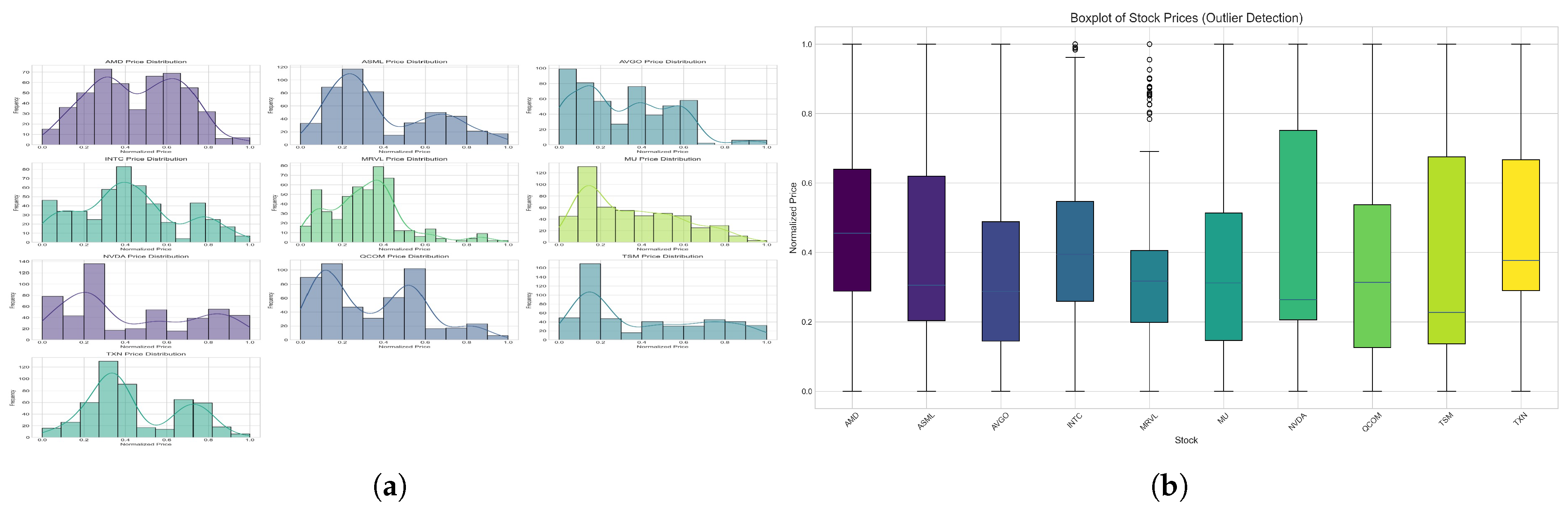
Figure 2.
A Stock Relationship Graph..
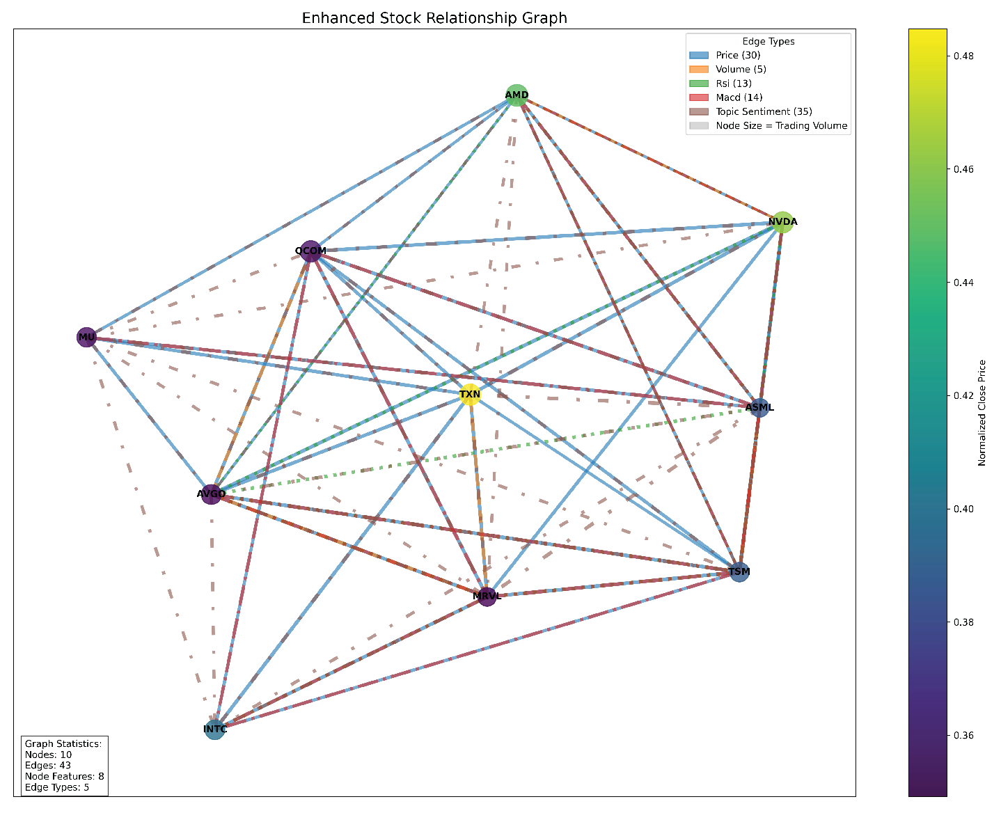
Figure 3.
Training and Validation History.

Figure 4.
Actual versus Predicted Prices.
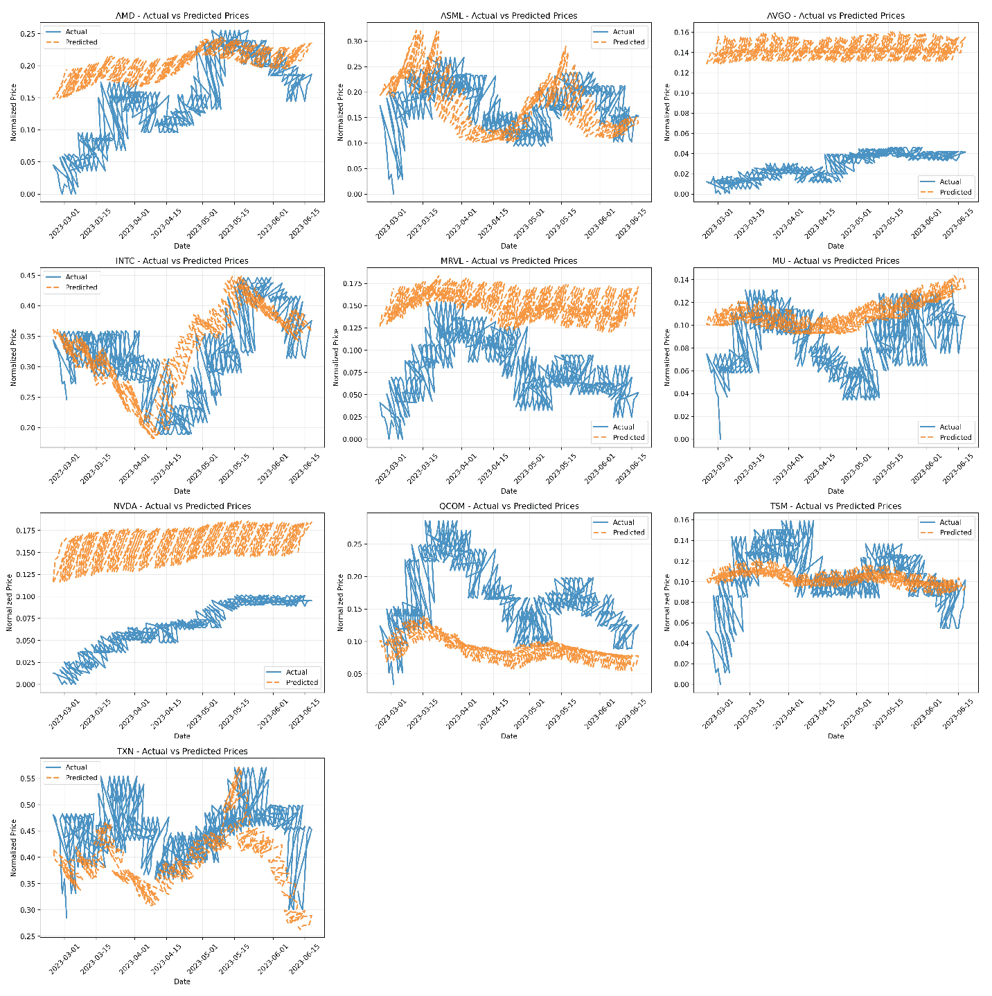
Figure 5.
Feature Importance Rankings.
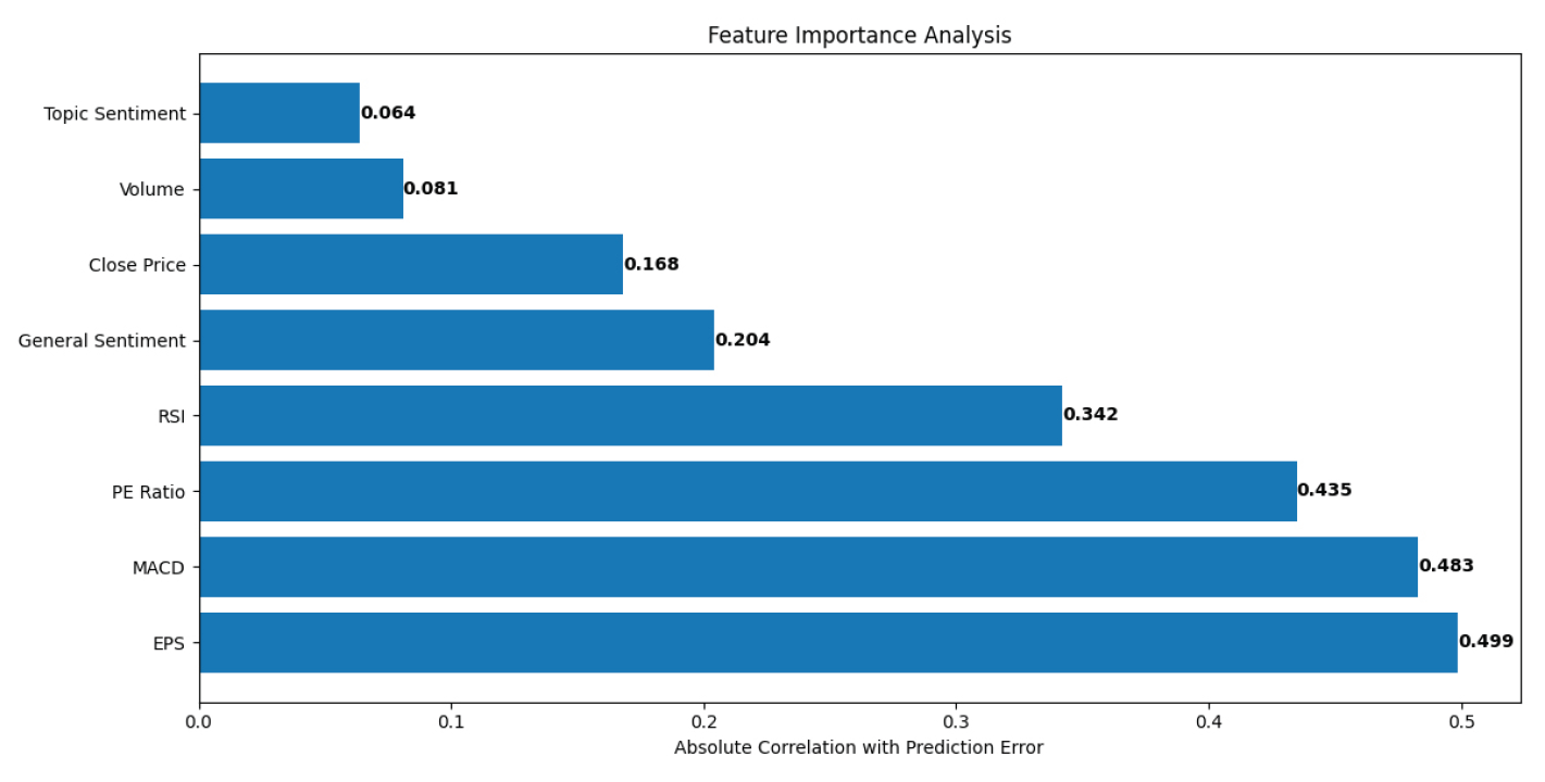
Figure 6.
RMSE Across Different Forecast Horizons.
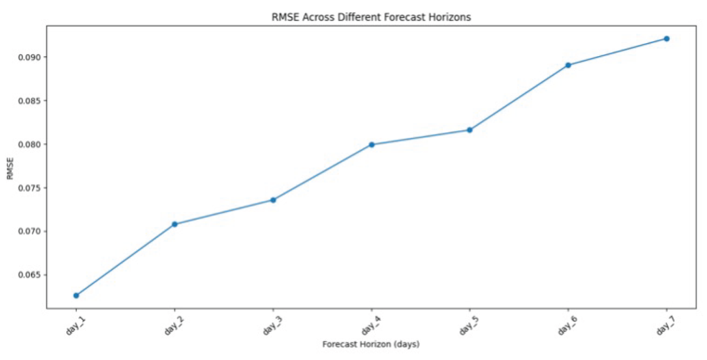
Figure 7.
RNNs’ LSTM and GRU Predictions.
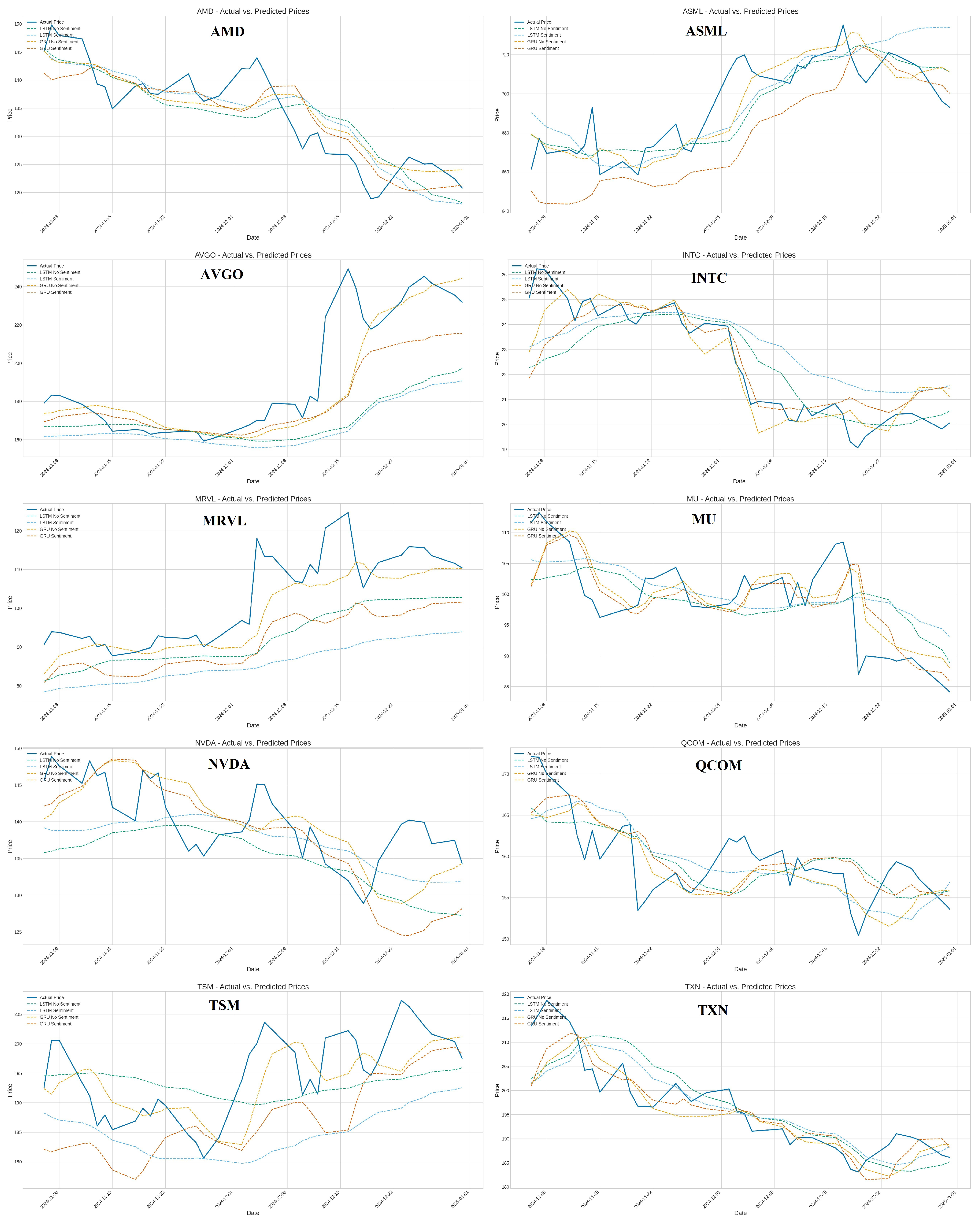
Figure 8.
ST-GNN Predictions.
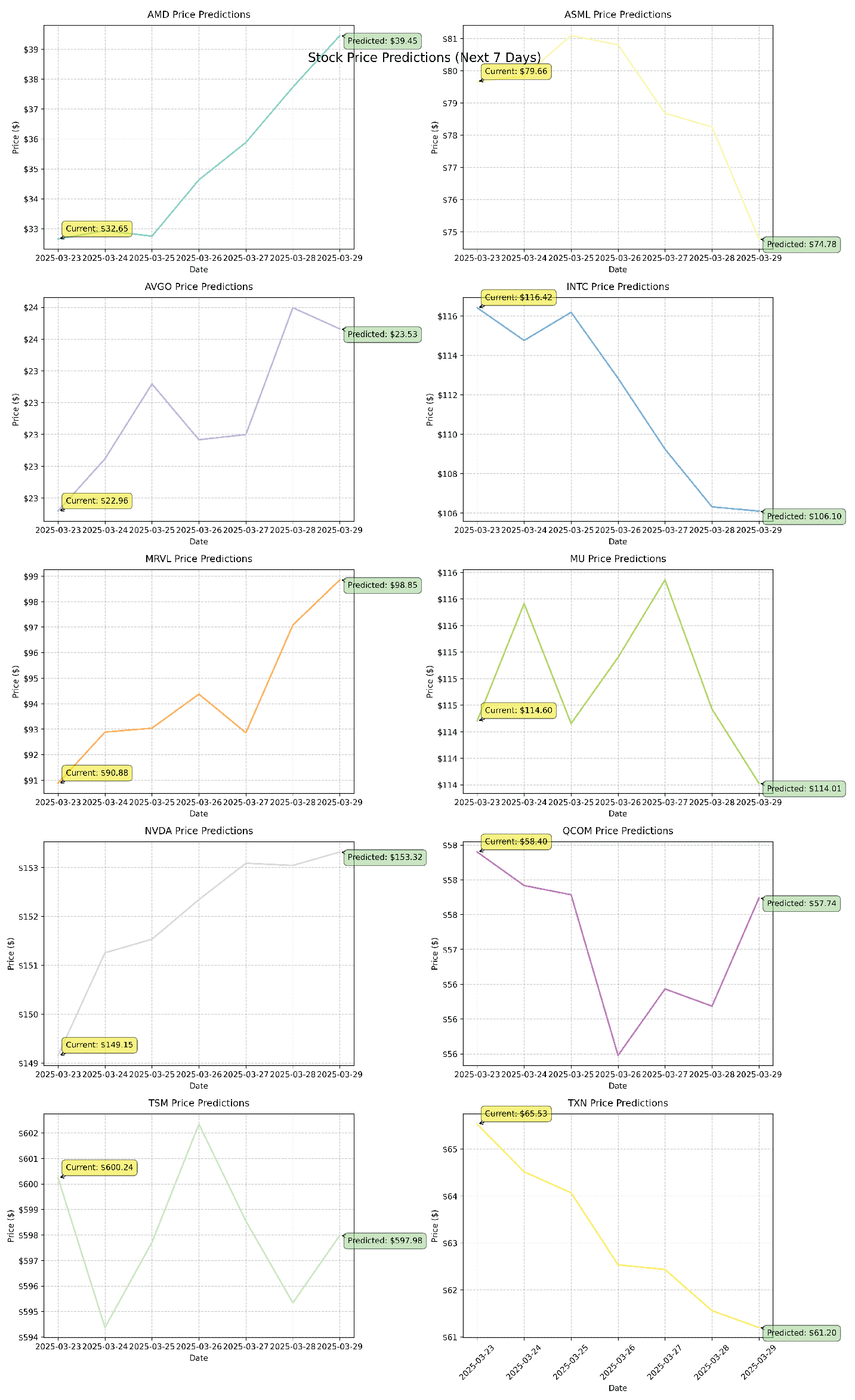

Table 1.
The performance metrics of LSTM and GRU.
| Metrics | Variant | Avg. RMSE | Avg. MAE | Avg. DA (%) | |
| Model | |||||
| GRU | no_sentiment | 6.67 | 4.86 | 58.16 | |
| GRU | forward_fill | 9.07 | 7.04 | 56.84 | |
| LSTM | no_sentiment | 9.46 | 7.29 | 55.00 | |
| LSTM | forward_fill | 10.71 | 8.64 | 55.00 | |
Disclaimer/Publisher’s Note: The statements, opinions and data contained in all publications are solely those of the individual author(s) and contributor(s) and not of MDPI and/or the editor(s). MDPI and/or the editor(s) disclaim responsibility for any injury to people or property resulting from any ideas, methods, instructions or products referred to in the content. |
© 2026 by the authors. Licensee MDPI, Basel, Switzerland. This article is an open access article distributed under the terms and conditions of the Creative Commons Attribution (CC BY) license (http://creativecommons.org/licenses/by/4.0/).
Copyright: This open access article is published under a Creative Commons CC BY 4.0 license, which permit the free download, distribution, and reuse, provided that the author and preprint are cited in any reuse.


