
Submitted:
26 February 2026
Posted:
26 February 2026
You are already at the latest version
Abstract
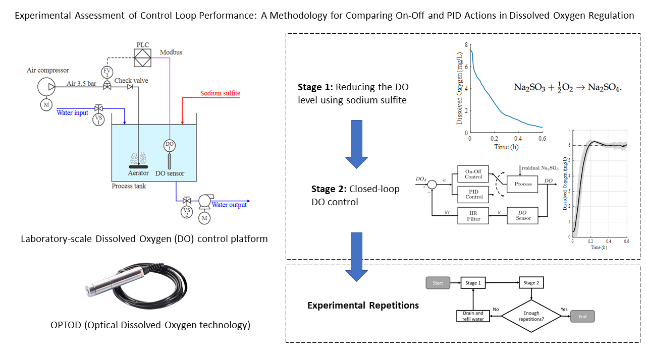
Experimental validation of dissolved oxygen (DO) control in aquaculture is often limited by biological variability, environmental factors, and pond hydrodynamics, which reduce reproducibility and hinder reliable assessment. To address this, we developed a laboratory-scale, control-oriented platform that minimizes external disturbances and enhances statistical reliability. Oxygen demand was emulated via chemical deoxygenation with sodium sulfite, so aeration experiments begin from near‑zero dissolved oxygen (DO). Sodium sulfite is added only during initialization; any residual persists briefly into the early closed-loop phase. Using this framework, On-Off control with hysteresis and discrete-time PID control were compared in terms of overshoot, rise time, settling time, and steady-state error. Under a confidence criterion, the PID controller required fewer repetitions than the On-Off strategy to achieve comparable reliability.
Keywords:
dissolved oxygen control
; experimental platform
; aquaculture automation
; PID control
; On-Off control
; programmable logic controller
; aeration systems
; reproducible experimentation
1. Introduction
The success of aquaculture depends on maintaining optimal water quality. Key parameters include pH, temperature, salinity, turbidity, and dissolved oxygen (DO), all of which directly affect metabolism, growth rate, feed conversion efficiency, and the survival of cultured organisms [1,2]. Among these variables, dissolved oxygen is widely recognized as a critical indicator of water quality, as it directly affects respiratory processes and the physiological performance of crustaceans [3]. Experimental and field studies have reported that DO concentrations below 5 mg/L induce significant physiological stress, reduce growth, and increase mortality in shrimp farming systems [1,4].
In aquaculture systems, dissolved oxygen dynamics are governed by the interaction of multiple factors, including biomass respiration, organic matter degradation, system hydrodynamics, mixing efficiency, and water temperature [5,6]. To mitigate hypoxic events, various aeration technologies have been developed, such as paddlewheel aerators, fine-bubble diffusers, venturi injectors, and mechanical surface aerators, each exhibiting specific operational characteristics and different oxygen transfer efficiencies [1,3,7]. However, the overall effectiveness of these devices depends not only on their mechanical design but also on the implemented control strategy and the availability of reliable, continuous dissolved oxygen measurements.
Accurate and real-time measurement of dissolved oxygen is therefore a fundamental requirement for aquaculture automation. Conventional chemical methods, such as Winkler titration and colorimetric techniques, provide acceptable accuracy for spot analyses but are unsuitable for continuous monitoring and closed-loop control applications due to their discrete nature and lack of direct integration with automatic control systems [8]. In contrast, electrochemical and optical dissolved oxygen sensors enable continuous digital data acquisition and integration into industrial automation and IoT-based architectures. Nevertheless, their practical performance strongly depends on signal conditioning, calibration procedures, temperature compensation, and the employed communication architecture [9,10].
In this context, laboratory-scale experimental platforms have become a key tool for research in smart aquaculture and aquatic process control [11,12,13,14]. These platforms allow the evaluation of different operational configurations representing real cultivation scenarios, such as variations in organic loading, thermal conditions, and turbidity levels [15,16]. Moreover, they facilitate systematic variable isolation, enabling controlled investigation of the individual effects of specific disturbances on dissolved oxygen dynamics, for instance by assessing aeration system performance under different temperature regimes or hydraulic mixing conditions [17,18]. Additionally, controlled experimental environments offer significant advantages, including reduced operational costs during the development phase, improved experimental reproducibility, and safe validation of advanced control algorithms prior to deployment in commercial production systems [9,19]. These characteristics align closely with current trends in smart aquaculture, which emphasize smaller-volume tanks, higher stocking densities, and extensive integration of monitoring and control technologies to ensure water quality while reducing energy and resource consumption [15,20].
Despite advances in automation and monitoring, a significant gap remains between large-scale production systems and experimental platforms used in research. In many commercial operations, aeration strategies continue to rely on empirical or time-based schemes without closed-loop feedback, leading to energy inefficiencies and suboptimal dissolved oxygen regulation [1,4]. Conversely, many laboratory studies employ low-cost hardware and non-industrial architectures, limiting robustness, scalability, and technological transferability of the obtained results [21,22]. This disconnect restricts systematic evaluation of advanced control strategies under controlled yet representative cultivation conditions.
Furthermore, conducting experimental studies using live organisms introduces inherent biological variability, ethical considerations, and risks to animal welfare, complicating reproducibility and rigorous validation of control algorithms [23]. To address this limitation, several studies have proposed the use of chemical oxygen scavengers, such as sodium sulfite, to induce controlled deoxygenation conditions in laboratory aquatic systems [23,24]. However, the practical application of this approach is nontrivial, as the theoretical reaction stoichiometry does not fully represent the actual conditions of potable water used experimentally. In addition, reaction kinetics depend on factors such as mixing intensity, water motion, and temperature, while reagent purity and storage conditions significantly influence experimental reproducibility [24].
Within this framework, the present work aims to design and construct a laboratory-scale experimental platform, oriented toward the modeling and control of dissolved oxygen dynamics in water. Beyond the platform development itself, the main contribution of this work lies in addressing a persistent gap in the existing literature, where clear, reproducible, and well-documented methodologies for the systematic study of aeration processes remain limited. The proposed framework integrates industrial-grade instrumentation, aeration systems, and a programmable logic controller, enabling real-time monitoring and implementation of control strategies under controlled experimental conditions. Carefully designed experimental protocols are conducted to achieve repeatable and reliable results, supported by consistent performance metrics. The proposed methodology and experimental dataset are intended to serve as a benchmark reference for future studies focused on the evaluation of alternative modeling approaches, aeration technologies, and control strategies in smart aquaculture and aquatic systems automation.
In summary, the main contributions of this work are:
- The design and implementation of an industrial-grade DO control platform, integrating a programmable logic controller (PLC), an optical dissolved oxygen sensor, and a proportional flow valve driven by a current controlled actuator.
- A reproducible experimental methodology for benchmarking control strategies under identical operating conditions, including repeated near-zero DO reset experiments, explicit signal conditioning, actuator saturation handling, and time domain performance metrics suitable for real world industrial deployment.
- Quantitative comparison of On–Off and PID control strategies based on performance indicators and a statistical approach to establish the necessary number of experimental repetitions.
The remainder of this article is structured as follows. Section 2 (Materials and Methods) describes the proposed experimental framework, including the design and construction of the laboratory-scale platform, the instrumentation employed, and the management methodology adopted. This section also details the control design and the experimental validation procedure. Section 3 presents the experimental results and discussions obtained under controlled operating conditions. Finally, the conclusions are presented in Section 4.
2. Materials and Methods
Our proposed framework is structured into three main stages with the objective of developing and validating a laboratory-scale experimental platform for the analysis and control of dissolved oxygen dynamics under reproducible conditions.
2.1. Experimental Platform and Management Methodology
This section addresses the design of a controlled experimental test bed integrating the process tank, aeration system, sensing and actuation hardware, and a programmable logic controller (PLC). A management methodology is defined to ensure repeatable operating conditions, including chemical DO depletion and standardized operating procedures. Data acquisition and signal conditioning are performed to provide reliable measurements for control-oriented analysis.
2.1.1. Physical Platform and Instrumentation Design
The experimental platform was conceived as a laboratory-scale, control-oriented test bed aimed at the systematic evaluation of DO control strategies under well-defined and repeatable conditions. Its architecture intentionally isolates the aeration process, allowing DO dynamics to be studied without the confounding effects typically present in full-scale aquaculture systems.
The main structure of the system is a rigid process tank (Figure 1), operating at a fixed working volume of 160 L. Together with the aerators and the DO sensor, this tank constitutes the core of the process in which DO concentration must be controlled. Water inflow is enabled only during preparation stages via the inlet line controlled by valve VS1, while discharge during cleaning and reset procedures is carried out through the outlet line actuated by valve VS2 and an auxiliary pump. During closed-loop operation, neither inflow nor outflow is active; both are used exclusively to replace the water between experiments.
Compressed air supplied by a pneumatic subsystem contains not only oxygen but also nitrogen, carbon dioxide, argon, and other trace gases. However, in the following analysis only oxygen is considered as the variable of interest. As shown in Figure 1, air is delivered by a compressor operating at a pressure of 3.5 bar. The stream passes through a flow control valve (FV1) and a check valve before reaching the submerged diffusers located at the bottom of the tank.
During preparation, sodium sulfite is manually added to the tank to induce controlled oxygen depletion. After preparation, dissolved oxygen was measured in real time using the Aqualabo OPTOD sensor, which operates with luminescent optical technology. Immersed in the tank, it provides the primary feedback variable for control. In this stage, a small amount of residual sulfite may remain and act as a transient oxygen-demand disturbance during closed-loop control. As shown in Figure 2, a programmable logic controller (PLC, Allen Bradley Micro 870) acquires these measurements via an RS-485 interface and executes the discrete-time control algorithm, generating actuation commands to FV1.
The analog control signal generated by the PLC is conditioned by a valve current driver and applied to an electropneumatic proportional valve (HF-PRO), which regulates the airflow supplied by the compressor to the submerged diffusers and constitutes the final control element of the aeration loop. The electrical architecture supporting the control loop is centralized around a 24 VDC power supply. Dedicated DC-DC converters generate the voltage levels required by the sensor, valve driver, and auxiliary components, while protective elements such as fuses are also included.
A summary of the main instrumentation and hardware specifications, including the key dimensioning parameters required for experimental replication, is provided in Table 1.
Together, Figure 1 and Figure 2 provide complementary views of the experimental platform, combining a process-oriented representation of air, water, and signal flows with an implementation-level description of the control, instrumentation, and power architecture supporting reproducible experimental validation of DO control strategies.
2.1.2. Platform Operation & Management Methodology
A structured operating and management methodology was defined to ensure repeatability, consistency, and traceability across experimental trials. The overall workflow adopted for the use of the experimental platform is summarized in the operational flow diagram, as shown in Figure 3, which outlines the preparation, control execution, and reset stages of each experiment.
Each experimental run begins with a preparation phase, during which the process tank is filled to the nominal operating volume of 160 L. The programmable logic controller (PLC) program is then deployed and executed, and correct acquisition of dissolved oxygen (DO) measurements from the sensor is verified before enabling any control action. During this phase, the system remains in preparation mode to prevent unintended aeration.
To establish a reproducible initial condition and emulate the oxygen consumption typically caused by biological activity in aquaculture systems, a chemical oxygen depletion procedure is applied. A fixed amount of 12 g of sodium sulfite () is manually added to the water. This compound reacts chemically with dissolved oxygen, progressively reducing the DO concentration until an anoxic condition is reached. It is worth noting that the natural decrease in DO, considering the maximum volume and initial aeration of the water, takes approximately 30 to 40 minutes. To accelerate this process, manual stirring was performed, reducing the DO level in less than 10 minutes. The number of manual mixing attempts ranged between four and five. Once the DO value approached zero, the water was allowed to rest for two minutes to stabilize the measurement. In this proposal, the deoxygenation step was standardized only to achieve a consistent low-DO initial condition, because the controlled aeration phase was the primary focus.
Once the target low-DO condition is achieved, the system transitions to the control execution phase. The selected control algorithm is activated within the PLC, and the platform operates in closed loop. During this phase, aeration is driven exclusively by the controller output. DO measurements and control signals are acquired in discrete time at a fixed sampling period and logged continuously for subsequent analysis.
After completion of each experimental run, a reset phase is performed. The aeration system is deactivated, the process tank is drained, and both the tank and the DO sensor are cleaned to remove residual sodium sulfite and prevent cross-test interference. This procedure ensures consistent initial conditions for successive experiments.
All data acquisition and signal handling are performed within the PLC. Raw DO measurements are internally scaled to engineering units before being used in control computations. To reduce the influence of measurement noise and short-term fluctuations inherent to dissolved oxygen sensing, a low-order digital filter is applied to the measured signal prior to its use in the control law. Both filtered and unfiltered signals are stored, allowing transparent offline analysis without affecting real-time execution.
Overall, this operating methodology ensures that experimental results are obtained under controlled and repeatable conditions, supporting the use of the platform as a laboratory-scale test bed for the experimental validation of dissolved oxygen control strategies.
2.2. Chemical Reduction of Dissolved Oxygen Using Sodium Sulfite
The proposed platform is designed to increase DO via aeration. Because it does not incorporate hardware to actively decrease DO (e.g., inert-gas sparging, vacuum degassing, or dedicated deoxygenation modules), a chemical oxygen scavenger was used to establish low-DO conditions for testing. Following standard practice for preparing a zero-DO solution for sensor calibration and low-oxygen checks, sodium sulfite () was selected as the reducing agent [25]. In aqueous media, sulfite consumes dissolved oxygen and is oxidized to sulfate according to:
Thus, the theoretical stoichiometry requires 1 mol of per 0.5 mol of removed. For a water volume L, the stoichiometric mass of sodium sulfite needed to remove an initial DO concentration (mg ) can be expressed as:
where is the molar mass of in mg and g is the molar mass of . In practice, the sulfite was added under mixing until the DO approached the target low level, and the final requirement was adjusted experimentally.
2.2.1. Implications of Using Potable Water (Chlorine Demand and Correction of the Theoretical Dose)
Potable water was used (160 L), which introduces an important practical correction: reacts not only with dissolved oxygen, but also with oxidants present in disinfected drinking water (e.g., free chlorine and chloramines). This additional demand can increase the required sulfite mass beyond the oxygen-only stoichiometric estimate in Eq. (2). The reactivity of sulfite toward chlorine species and the broader implications of sulfite-based dechlorination/quencher chemistry have been documented in peer-reviewed studies [26,27,28]. Therefore, rather than relying solely on stoichiometry, the sulfite dose was determined using a two-step approach:
- Initial stoichiometric estimate: compute the oxygen-only requirement from Eq. (2) using the measured initial DO.
- Experimental correction in potable water: apply the estimated dose under agitation and verify whether the measured DO reaches the intended low value. If not, add incremental sulfite until the target DO is achieved, thereby capturing the additional oxidant demand of the potable water matrix [26,27,28].
2.3. Data Acquisition, Pre-Processing, and Control
The aeration control system begins with sampling the signal to determine the preprocessing of the measurements, which establishes the basis for the subsequent control actions. It considers mainly a desired dissolved oxygen setpoint (), a controller, a process, a DO sensor, and a IIR filter, as shown in Figure 4. The implementation treats the process model as a black-box, where the input is the control effort, represented by the valve aperture, with a maximum value limited by the 3.5 bar threshold of the valve, see Table 1, while the output is the DO measurement.
2.3.1. Sampling and Preprocessing of Dissolved Oxygen Measurements
The experiments were conducted under controlled laboratory conditions using the experimental platform described in Section 2.1.2. The water temperature was maintained at approximately 20–, and a fresh volume of potable water was supplied for each run. The DO sensor was positioned 12 cm from the tank border with an immersion depth of 20 cm, while two diffusers were fixed at the base in equidistant positions on opposite sides. During each measurement, both the inlet and outlet valves remained closed to ensure stable hydraulic conditions.
Under our laboratory conditions, the initial DO measurements ranged from 0 to 7.8 mg/L. Each aeration experiment lasted 1 h and 15 min, whereas the DO depletion phase exhibited variable duration, being terminated once the concentration approached zero.
For the DO measurement at discrete instants , a first-order infinite impulse response (IIR) filter was implemented to attenuate noise by smoothing the experimental data [29]. The discrete-time representation of the filter is given in Equation (3):
where denotes the filtered output at instant k, and is a forgetting factor close to one that determines the relative weight of past and current measurements [30]. Henceforth, the filtered signal will be employed in our analysis during both the DO decay stage and the controlled aeration stage. For simplicity, will be referred to as DO, whereas y will denote the raw DO measurement.
For the controlled aeration stage using PID, an experiment is required to obtain a reaction curve, which is subsequently described in Section 2.3.3. To this end, a sigmoidal adjustment is proposed by means of a logistic function:
where L denotes the maximum asymptotic value, the slope parameter, and the inflection point of the curve. To estimate these parameters, the following cost function is minimized using the least squares method . Therefore, the optimal parameters are .
2.3.2. On-Off Control Design
As part of the control strategies, an On-Off controller is proposed. This approach ensures low computational cost and straightforward implementation. The controller operates by switching between open and closed states according to the sensor measurement relative to the reference value [31].
This control strategy employs hysteresis, which prevents excessive switching and thereby protects the equipment during tests. The hysteresis band (mg/L) is determined by control requirements, as well as by the characteristics of the sensor, actuator, and volume of water. The valve aperture () is fully open when the filtered DO value () is below the desired value (), and fully closed when the measurement exceeds the desired value, as detailed below.
The implementation of this controller considers only the positive error, leading to the oxygen inflow. In this case, this characteristic is suitable because the proposed system does not extract oxygen. In terms of security, the correct selection of hysteresis protects the system electrically and mechanically.
2.3.3. PID Controller Design via Ziegler–Nichols Method
The continuous-time control law implemented for the PID controller is given by
where denotes the valve aperture, is the control error, and , , and are the proportional, integral, and derivative gains, respectively.
For implementation purposes, the control law is discretized using a fixed sampling time , which is independent of the specific hardware platform employed. The discrete-time representation of the PID controller is expressed as
The tuning of the PID controller is performed using the Ziegler–Nichols (ZN) method [31,32,33]. The procedure involves fitting the experimental data of a system reaction curve to a sigmoidal function, which is obtained from a step input experiment, see Figure 5(left), combined with data treatment based on filtering and sigmoidal fitting shown in Section 2.3.1. Two key parameters of this sigmoidal curve must be determined geometrically: the delay time (L) and the time constant (T). The slope of the tangent at the inflection point defines the reaction rate (R), with , see Figure 5(right).
The relationship between the Ziegler-Nichols parameters and the controller gains is given by and . It is worth mentioning that the classical Ziegler-Nichols method employs a first-order plus dead-time approximation of the reaction curve. In our case, however, a sigmoidal fitting was adopted since it provided a more consistent representation of the experimental data.
2.4. Statistical Criterion for Determining the Number of Experimental Repetitions
The control system is evaluated using standard performance metrics: overshoot, rise time , defined as the time required for the measured DO concentration to increase from 10% to 90% of the reference value, settling time , defined as the time required for the DO concentration to enter and remain within a band around the reference, and the mean steady-state error , calculated as , where (mg/L) denotes the instantaneous error at sample k once the system has reached steady state, and is the number of samples considered in that regime.
In order to determine the number of repetitions required to obtain a statistically reliable estimate of the steady-state mean error , a confidence-interval-based precision criterion was adopted [34]. Let denote the mean steady-state error obtained in the experiment i-th. Therefore, the mean error of N independent repetitions, denoted by is defined as
Therefore, the corresponding standard deviation of the experiments is
so that, the standard error of the mean is defined as
Assuming approximate normality of the estimator, a two-sided confidence interval (CI) for the true mean error is computed using the Student’s t distribution, that is , with , where denotes the critical value with degrees of freedom. The quantity represents the semi-width of the confidence interval and provides a direct measure of estimation precision [35].
Therefore, a practical stopping criterion can be defined by selecting the minimum number of repetitions N such that , where is a predefined tolerance on the admissible uncertainty of the estimated mean error [34].
3. Results and Discussions
3.1. Implementation of the Experimental Platform and Management Methodology
The experimental platform developed in this work was successfully implemented and operated as a laboratory-scale test bed for DO control experiments. The final system integrates the process tank, pneumatic aeration subsystem, sensing instrumentation, control hardware, and power distribution into a compact and functional structure, as shown in Figure 6. The implemented platform is consistent with the proposed design and enabled systematic experimentation under controlled conditions.
The process tank operated at a nominal working volume of 160 L in all experimental trials. Water handling components allowed reliable filling and draining between experiments, while the pneumatic subsystem operated without mechanical faults, providing consistent air delivery during closed-loop operation.
The sensing and control infrastructure functioned reliably throughout the experiments. The optical DO sensor provided continuous measurements, and stable RS-485 communication with the programmable logic controller (PLC) ensured uninterrupted data acquisition. Control execution within the PLC was performed in discrete time, with actuation commands continuously applied to the proportional valve.
The chemical oxygen depletion procedure based on the manual addition of 12 g of sodium sulfite () consistently reduced the DO concentration to low levels prior to control activation. Similar depletion behavior was observed across repeated trials, confirming the reproducibility of the selected dosing and mixing procedure.
Transitions between preparation, closed-loop operation, and reset phases were achieved without operational discontinuities. The reset procedure, involving tank draining and sensor cleaning, enabled recovery of comparable initial conditions between experiments. Dissolved oxygen measurements, control signals, and time stamps were logged continuously in all trials, supporting offline analysis. Basic signal conditioning reduced short-term measurement fluctuations while preserving the dominant process dynamics.
Overall, the obtained results confirm that the implemented platform and its associated management methodology provide a reliable and reproducible laboratory-scale environment for the experimental validation of dissolved oxygen control strategies.
3.2. Results of Dissolved Oxygen Control
Considering the platform above, this work uses the two mentioned controller methods to compare the results under the same conditions. The objective of each test is to track a desired DO level by regulating the valve aperture. The sensor measurements were filtered using an IIR filter with a forgetting factor of . In this system, the increase in DO is determined by the valve, while sulfite determines the drop. Before control initialization, the DO level was reduced to a value close to zero by adding 12 g of sodium sulfite, exceeding the 9.3 g required by stoichiometry, due to the use of potable water instead of pure water, as described in Section 2.2.
This reduction in DO is difficult to model because, in addition to the appropriate amount of sodium sulfite, it depends on water movement, which can accelerate the reaction through superficial aeration. Furthermore, the reduction in DO also depends on the initial DO value, which itself is influenced by the water flow rate when filling the tank. Figure 7 (left) illustrates three examples of DO reduction from a high initial value. In Test 1, a typical decay is observed without water agitation. In Tests 2 and 3, the reduction occurs more rapidly due to agitation. However, in Test 2, a slight increase can be observed after 0.2 h, caused by aeration generated by water agitation. Altogether, these observations highlight the need to conduct experiments under the same initial DO condition, close to zero, prior to controlled aeration evaluated in Section 3.2.1 and Section 3.2.2, in order to reach repeatability under laboratory conditions.
In this empirical adjustment of the required amount of sodium sulfite, it is difficult to ascertain whether, when a DO value close to zero is measured, residual sodium sulfite remains in the water, ready to react once the water is aerated. Figure 7(right) illustrates a typical aeration process under such excess conditions (about 20 g), where sodium sulfite reacts immediately upon air introduction, producing abrupt changes in the DO measurement from the outset, as both the increase in DO and the simultaneous consumption of sodium sulfite occur together.
For both control approaches, this study performed 10 tests for each to evaluate the consistency of their responses.
3.2.1. Results of the On-Off Control Strategy
The On-Off control employs 5% hysteresis with respect to mg/L (i.e. mg/L). In this case, the 10 tests last approximately 1.3 hours to track the DO setpoint. Sodium sulfite provides a repeatable oxygen demand disturbance that reduces DO in the bench system. This controller provided a fair response in tracking the reference throughout the test. In Figure 8 and Figure 9, note that the peaks reached in each test are produced due to the delay effect of the aerator. The DO level continues to rise despite the control valve being completely closed. Conversely, the minimum peak corresponds to the drop in DO caused by the sulfite reaction when the valve is opened to regulate the DO level.
Table 2 summarizes the performance obtained in each test using the proposed controller. In terms of overshoot, the average is (mg/L), with a maximum of (mg/L) in test 5 and a minimum of (mg/L) in test 4. The settling time has an average of 451.4 seconds (0.125 hours) with a minimum of 339 and a maximum of 595 at tests 3 and 4, respectively. On the other hand, the average rising time is 355.4 seconds (0.099 hours), with a maximum of 523.5 at test 4 and a minimum of 291 at test 3. Finally, the maximum mean error was observed in test 5, while the minimum occurred in test 10. These On-Off control performance results can be adjusted depending on the value of the hysteresis band H[31].
3.2.2. Results of the PID Control Strategy
The second controller proposed by this work is the PID control algorithm. In this case, the test bench uses all the same conditions considered in the previous controller. The Ziegler-Nichols method is applied in the reaction curve, shown in Figure 10, to obtain the proportional , integral , and derivative gains , with and .
Figure 10 illustrates the system’s reaction curve, as presented in Section 2.3.3. The gray dots represent the response to a step input until steady state, while the green line corresponds to the filtered data obtained using the discrete filter described in Equation (3). The adjusted sigmoidal reaction curve is shown as the blue line, derived from Equation (4).
Figure 11 and Figure 12 illustrate the responses obtained by implementing the PID controller in the system. The setpoint remains at 6 mg/L, considering the same amount of sulfite in the tank. Each test shows a minimum peak generated due to the reaction of the sulfite with water when the aerator is activated. Compared with the On-Off, the responses do not exhibit oscillations, and the behavior is smoother.
Table 3 presents the performance metrics of the PID implementation. The maximum overshoot is (mg/L) at test 5; meanwhile, the minimum is (mg/L) at test 4, with an average of (mg/L). The average rising time is 394.3 seconds (0.11 hours), with a maximum of 505 seconds recorded in test 4 and a minimum of 340.5 seconds recorded in test 1. In terms of settling time, the average is 521.5 seconds, with a maximum of 651 (test 4) and a minimum of 446.5 (test 3), respectively. Finally, the maximum mean error was observed in test 4, while the minimum was observed in test 9.
The Z–N method was used as a standardized baseline; further fine-tuning was not pursued to keep methodology comparable and replicable. Therefore, these PID control results can be improved with more advanced tuning alternatives and other, more robust control strategies [31,36].
During the control tests, the PID controller shows lower steady-state error and variability under the tested conditions compared to the On–Off controller, see Table 4, particularly in the steady state. In the transient state, however, the settling time of both controllers is similar, since the PID controller saturates at 100% owing to the large error, see Figure 12. It is difficult to draw definitive conclusions in this regime, partly because it is further influenced by the residual sodium sulfite. In practical applications, however, it is the steady state that is most relevant.
3.3. Numerical Evaluation of the Required Number of Repetitions
The confidence interval based criterion was applied to the On-Off and PID controllers in order to determine the number of repetitions required for each case to obtain a reliable estimate of the steady-state mean error. The analysis follows the procedure described in Section 2.4. The required number of independent experimental repetitions was determined using a two-sided confidence interval.
For each controller, the minimum N (number of Test) was selected such that the confidence interval semi-width satisfies the practical accuracy criterion where mg/L is the reference value. This condition ensures that the estimation uncertainty remains within of the reference.
For the On-Off controller, the minimum number of repetitions satisfying this requirement was , whereas for the PID controller only repetitions were required. Table 4 summarizes the corresponding steady-state error mean , the standard error , the confidence semi-width , and the relative error with respect to the reference.
It can be observed that, under the selected tuning and experimental conditions, the PID controller exhibits lower dispersion and therefore requires fewer repetitions to achieve the same statistical confidence level. However, this comparison should be interpreted as referential. Each controller may improve its performance and variability characteristics through further tuning adjustments. Consequently, the purpose of this analysis is not to establish a strict superiority of one control strategy over the other, but rather to illustrate a systematic and statistically grounded procedure for determining the sufficient number of experimental repetitions in each case.
3.4. Limitations and Future Work
An interesting observation regarding DO regulation under On-Off control is that each oscillation exhibits a downward slope proportional to the residual sodium sulfite, as illustrated by the yellow dashed line in Figure 13 (left) following the initialization stage. Consequently, during the third oscillation, the variation in DO level becomes nearly constant, indicating that the sodium sulfite has been almost completely consumed. In other words, the disturbance generated in the aeration system due to the residual sodium sulfite is temporary, lasting on average three cycles in the steady state under On-Off control, although it is also expected to occur under PID control. Future work could focus on developing a methodology that not only reduces DO to its minimum value but also eliminates residual sodium sulfite prior to aeration control, thereby reducing the error variance observed in Figure 13 (middle and right).
Furthermore, in this study, we assumed that the amount of air supplied by the diffusers is proportional to the valve aperture. However, this relationship is not strictly linear in real applications. According to the technical specifications of both the air compressor and the diffusers, the dependence between these parameters is nearly linear across most operating ranges, but becomes nonlinear at the extremes. As future work, we suggest modeling this nonlinear behavior at the boundaries, using some data based modeling method [30,37,38]. Moreover, data acquisition was carried out at a sampling frequency of 2 Hz ( s), which corresponds to the maximum rate permitted by the sensor. This rate can subsequently be reduced to lower the computational cost, where the minimum sampling rate value must satisfy the Nyquist criterion.
Finally, the results presented in this work encourage us to further complicate the problem by introducing disturbances into the system, such as varying the pond temperature or including living species in the tank. In addition, the aeration mechanism could be replaced with one that generates significant mass movement [11], so that new and more advanced control strategies can be studied on the platform proposed in this paper.
4. Conclusions
This paper presents a reproducible laboratory-scale benchmark for dissolved oxygen regulation that reduces environmental and biological variability while preserving the essential dynamics of aeration-based DO control. Using chemical deoxygenation to enforce comparable initial conditions, the platform enables statistically grounded comparison of two control strategies across repeated trials. The experiments show that On–Off control with hysteresis provides a simple and robust baseline but produces larger steady-state variability, whereas discrete-time PID achieves tighter regulation and smoother behavior under the same operating conditions. Beyond highlighting performance differences, the proposed methodology makes it possible to determine how many repetitions are needed to reach a targeted confidence level in estimated tracking metrics, supporting more reliable controller evaluation prior to field deployment. Finally, the framework is positioned as a baseline for future extensions, including protocols that remove residual sulfite effects prior to control activation, inclusion of controlled disturbances such as temperature variation, and systematic testing of alternative aeration mechanisms and advanced strategies such as adaptive and predictive control.
Author Contributions
Conceptualization, J.M. and E.J.; methodology, J.M., S.P., A.G., and E.J.; software, J.M.; validation, J.M.; formal analysis, J.M. and E.J.; investigation, J.M. and E.J.; resources, J.M.; data curation, J.M.; writing original draft preparation, J.M., S.P., A.G., and E.J.; writing, review and editing, J.M., S.P., A.G., and E.J.; visualization, J.M., S.P., A.G., and E.J.; supervision, E.J.; project administration, E.J.; funding acquisition, E.J. All authors have read and agreed to the published version of the manuscript.
Funding
This research was funded by CONCYTEC PROCIENCIA for the development carried out within the framework of the Applied Research Project: Code E041-2023-02, Contract No. PE501082364-2023.
Data Availability Statement
The data presented in this study are openly available at GitHub repository https://github.com/jmagallanesc92/DO-Control.
Conflicts of Interest
The authors declare no conflicts of interest.
References
- Boyd, C.E. Water Quality: An Introduction; Springer, 2015. [Google Scholar] [CrossRef]
- Boyd, C.E.; Tucker, C.S. Pond Aquaculture Water Quality Management; Springer, 1998. [Google Scholar]
- Colt, J. Computation of dissolved gas concentrations in water as functions of temperature, salinity and pressure. American Fisheries Society Special Publication 1984, 14, 1–154. [Google Scholar]
- FAO. The State of World Fisheries and Aquaculture 2020: Sustainability in Action; Food and Agriculture Organization of the United Nations: Rome, Italy, 2020. [Google Scholar]
- Summerfelt, S.T. Design and management of conventional fluidized-sand biofilters. Aquacultural Engineering 2006, 34, 275–302. [Google Scholar] [CrossRef]
- Malone, R.F.; Pfeiffer, T.J. Rating fixed film nitrifying biofilters used in RAS. Aquacultural Engineering 2006, 34, 389–402. [Google Scholar] [CrossRef]
- Jayanthi, M.; Balasubramaniam, A.; Suryaprakash, S.; Veerapandian, N.; Ravisankar, T.; Vijayan, K. Assessment of standard aeration efficiency of different aerators and its relation to the overall economics in shrimp culture. Aquacultural Engineering 2021, 92, 102142. [Google Scholar] [CrossRef]
- APHA. Standard Methods for the Examination of Water and Wastewater, 23rd ed.; American Public Health Association, 2017. [Google Scholar]
- Yu, M.; Feng, Y.; Ouyang, B.; Wills, P.S.; Tang, Y. Dissolved oxygen in aquaculture ponds: Causal factors, predictive modeling, and intelligent monitoring. Aquacultural Engineering 2026, 112, 102634. [Google Scholar] [CrossRef]
- Rastegari, H.; Nadi, F.; Lam, S.S.; Ikhwanuddin, M.; Kasan, N.A.; Rahmat, R.F.; Mahari, W.A.W. Internet of Things in aquaculture: A review of the challenges and potential solutions based on current and future trends. Smart Agricultural Technology 2023, 4, 100187. [Google Scholar] [CrossRef]
- Cahua, D.; Antezana, F.; Palomino, S.; Alegria, E.J. Prototype Aeration System for Dissolved Oxygen Control Using a Paddle Wheel Mechanism. In Proceedings of the 2025 16th IEEE International Conference on Industry Applications (INDUSCON), 2025; pp. 16–21. [Google Scholar] [CrossRef]
- Chiotti, D.; Quispe, M.; Quino, G.; Alegria, E.J. Precision Aquaculture Feeder for Floating Platforms Considering Inertial Disturbances. In Proceedings of the 2025 IEEE 7th Colombian Conference on Automatic Control (CCAC), 2025; pp. 1–6. [Google Scholar] [CrossRef]
- Quispe, M.; Chiotti, D.; Alegria, E.J. A Dual-Arm Rotational Robotic Manipulator with a Dynamically-Driven Non-Actuated Joint for Smart Aquaculture. In Proceedings of the 2025 IEEE 7th Colombian Conference on Automatic Control (CCAC), 2025; pp. 1–6. [Google Scholar] [CrossRef]
- Quispe, M.; Chiotti, D.; Del-Águila, J.; Quino, G.; Jara Alegria, E. Automatic pellet positioner with switched fuzzy-PD control for a smart shrimp feeder. Smart Agricultural Technology 2026, 13, 101863. [Google Scholar] [CrossRef]
- Badiola, M.; Mendiola, D.; Bostock, J. Recirculating Aquaculture Systems (RAS) analysis: Main issues on management and future challenges. Aquacultural Engineering 2012, 51, 26–35. [Google Scholar] [CrossRef]
- Timmons, M.B.; Ebeling, J.M. Recirculating Aquaculture, 4th ed.; Cayuga Aqua Ventures, 2018. [Google Scholar]
- Wu, Y.; Liu, Z.; Zhang, H.; Li, X. Experimental Measurements on the Influence of Inlet Pipe Configuration on Hydrodynamics and Dissolved Oxygen Distribution in Circular Aquaculture Tank. Water 2025, 17, 2172. [Google Scholar] [CrossRef]
- Zhou, X.; Wang, J.; Huang, L.; Li, D.; Duan, Q. Modelling and controlling dissolved oxygen in recirculating aquaculture systems based on mechanism analysis and an adaptive PID controller. Computers and Electronics in Agriculture 2022, 192, 106583. [Google Scholar] [CrossRef]
- Ren, Q.; Wang, X.; Li, W.; Wei, Y.; An, D. Research of dissolved oxygen prediction in recirculating aquaculture systems based on deep belief network. Aquacultural Engineering 2020, 90, 102085. [Google Scholar] [CrossRef]
- Food and Agriculture Organization of the United Nations. The State of World Fisheries and Aquaculture 2018: Meeting the Sustainable Development Goals. Technical report; Food and Agriculture Organization of the United Nations, 2018. [Google Scholar]
- Singh, M.; Sahoo, K.S.; Gandomi, A.H. An Intelligent-IoT-Based Data Analytics for Freshwater Recirculating Aquaculture System. IEEE Internet of Things Journal 2024, 4206–4217. [Google Scholar] [CrossRef]
- Chiu, M.C.; Yan, W.M.; Bhat, S.A.; Huang, N.F. Development of smart aquaculture farm management system using IoT and AI-based surrogate models. Journal of Agriculture and Food Research 2022, 9, 100357. [Google Scholar] [CrossRef]
- Durdevic, P.; Raju, C.S.; Yang, Z. Potential for Real-Time Monitoring and Control of Dissolved Oxygen in the Injection Water Treatment Process. IFAC-PapersOnLine 2018, 51, 170–177. [Google Scholar] [CrossRef]
- Kwon, H.J.; Jeong, J.S. Clearing up the oxygen dip in HPAEC–PAD sugar analysis: Sodium sulfite as an oxygen scavenger. Journal of Chromatography B 2019, 1128, 121759. [Google Scholar] [CrossRef]
- Porfert, C. QA Bulletin: Calibration of Dissolved Oxygen Meters. Technical Report EQAGUI-DO, Revision 0, United States Environmental Protection Agency (EPA) New England, Office of Environmental Measurement and Evaluation; Quality Assurance Unit, 2006. [Google Scholar]
- Bedner, M.; MacCrehan, W.A.; Helz, G.R. Making chlorine greener: Investigation of alternatives to sulfite for dechlorination. Water Research 2004, 38, 2505–2514. [Google Scholar] [CrossRef]
- Moore, N.; Ebrahimi, S.; Zhu, Y.; Wang, C.; Hofmann, R.; Andrews, S. A comparison of sodium sulfite, ammonium chloride, and ascorbic acid for quenching chlorine prior to disinfection byproduct analysis. Water Supply 2021, 21, 2313–2323. [Google Scholar] [CrossRef]
- Li, X.; et al. A Review of Traditional and Emerging Residual Chlorine Quenchers for Disinfection Byproduct Research. Toxics 2023, 11, 410. [Google Scholar] [CrossRef]
- Proakis, J.G.; Manolakis, D.G. Digital Signal Processing: Principles, Algorithms, and Applications, 5th ed.; Pearson Education: Hoboken, NJ, 2022. [Google Scholar]
- Alegria, E.J.; Bottura, C.P. Data-Based Local Smoothing Technique for Parameters Estimation of Nonlinear ARX Models. In Proceedings of the 2019 American Control Conference (ACC), 2019; pp. 4350–4355. [Google Scholar] [CrossRef]
- Ogata, K. Modern Control Engineering, 5th ed.; Prentice Hall: Upper Saddle River, NJ, 2010. [Google Scholar]
- Ziegler, J.G.; Nichols, N.B. Optimum Settings for Automatic Controllers. Transactions of the ASME 1942, 64, 759–768. [Google Scholar] [CrossRef]
- Franklin, G.F.; Powell, D.; Emami-Naeini, A. Feedback Control of Dynamic Systems, 8th ed.; Pearson: Harlow, England, 2019. [Google Scholar]
- Montgomery, D.C.; Runger, G.C. Applied Statistics and Probability for Engineers, 7th ed.; John Wiley & Sons, 2018. [Google Scholar]
- Box, G.E.P.; Hunter, J.S.; Hunter, W.G. Statistics for Experimenters: Design, Innovation, and Discovery, 2 ed.; Wiley-Interscience: Hoboken, NJ, 2005. [Google Scholar]
- Borase, R.P.; Maghade, D.K.; Sondkar, S.Y.; Pawar, S.N. A review of PID control, tuning methods and applications. International Journal of Dynamics and Control 2021, 9, 818–827. [Google Scholar] [CrossRef]
- Alegria, E.J.; Giesbrecht, M.; Bottura, C.P. Causal regression for online estimation of highly nonlinear parametrically varying models. Automatica 2021, 125, 109425. [Google Scholar] [CrossRef]
- Alegria, E.; Giesbrecht, M.; Bottura, C. An associative-memory-based method for system nonlinearities recursive estimation. In Automatica; Publisher Copyright: © 2022 Elsevier Ltd, 2022; Volume 142. [Google Scholar] [CrossRef]
Figure 1.
Functional architecture and integrated air, water, and signal flows of the experimental DO control platform.
Figure 1.
Functional architecture and integrated air, water, and signal flows of the experimental DO control platform.
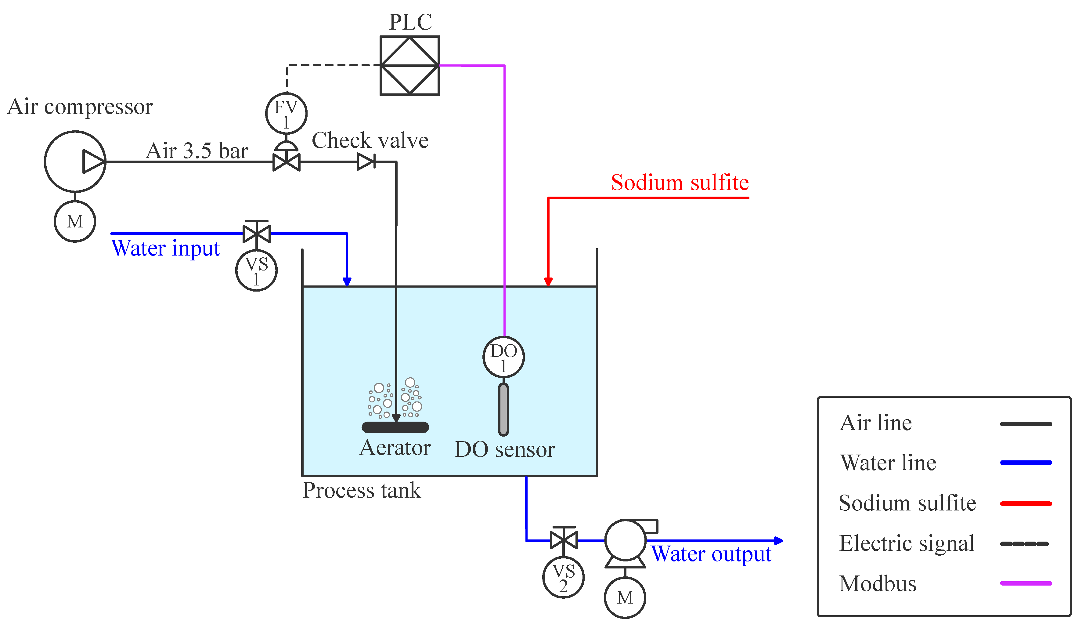
Figure 2.
Control and instrumentation architecture of the experimental DO control platform.
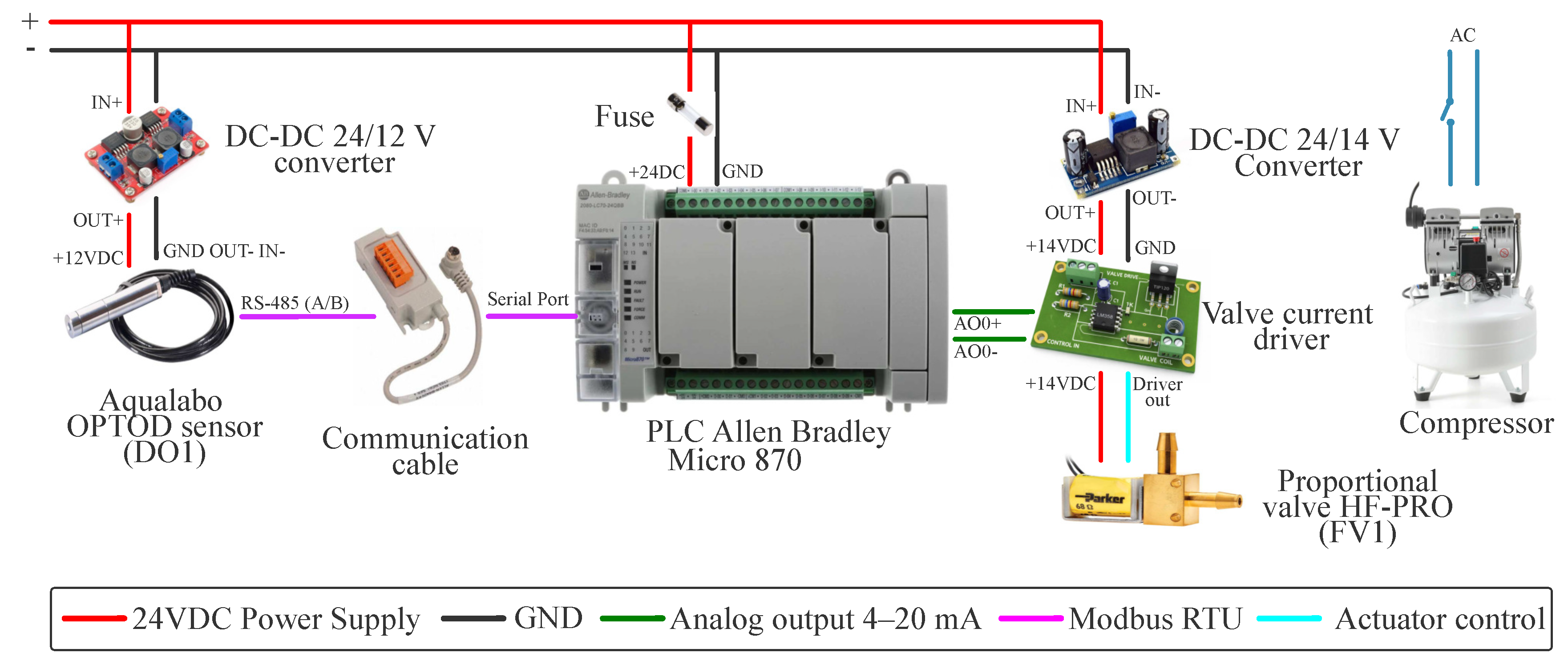
Figure 3.
Operational workflow for experimental execution on the DO control platform.
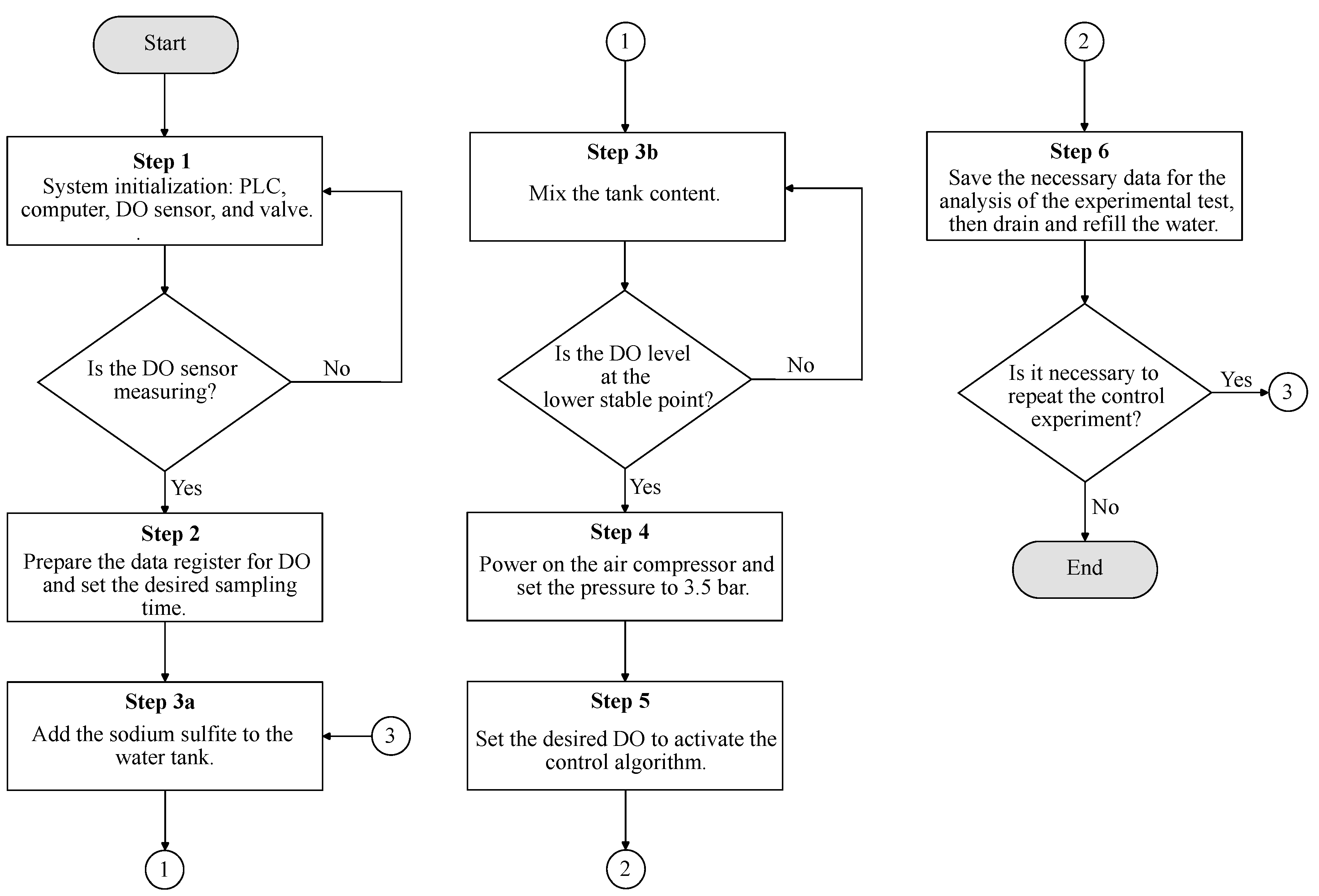
Figure 4.
Block diagram of the feedback aeration control system.
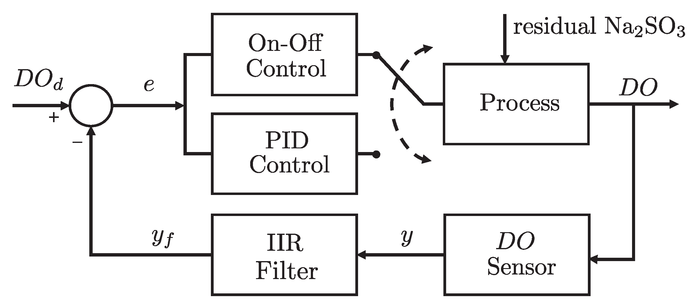
Figure 5.
Step input signal (left) and corresponding reaction curve with Z-N parameters (right).
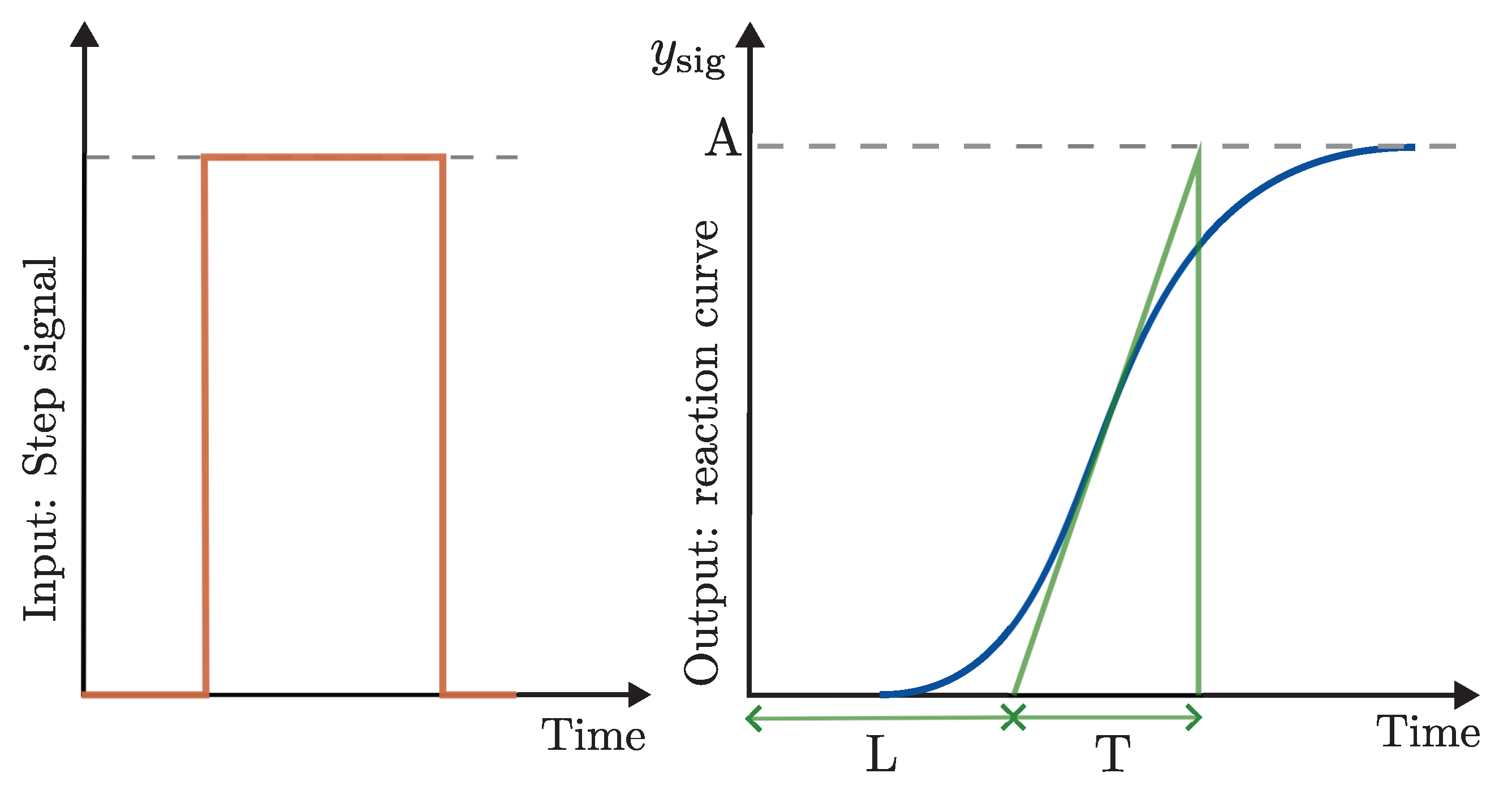
Figure 6.
Implemented experimental platform for dissolved oxygen control experiments: front and top views.
Figure 6.
Implemented experimental platform for dissolved oxygen control experiments: front and top views.
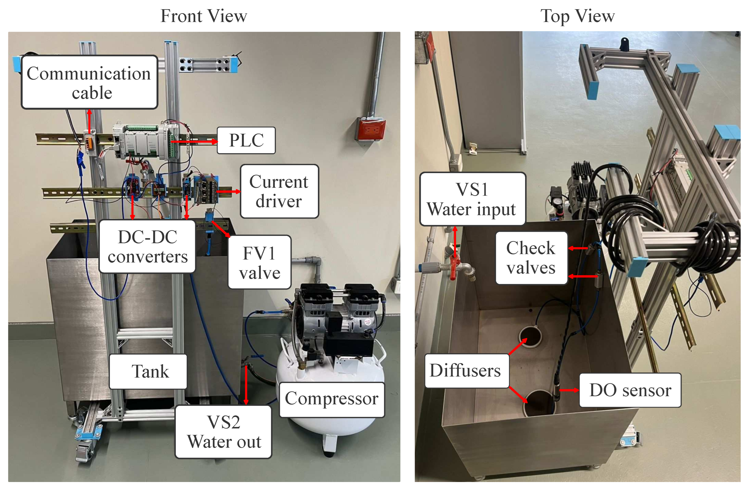
Figure 7.
Example of three typical DO decay curves, starting from the high values characteristic of freshly collected drinking water and decreasing to a minimum due to reaction with sodium sulfite (left), and typical DO evolution when an excessive amount of sodium sulfite (about 20 g) is added (right).
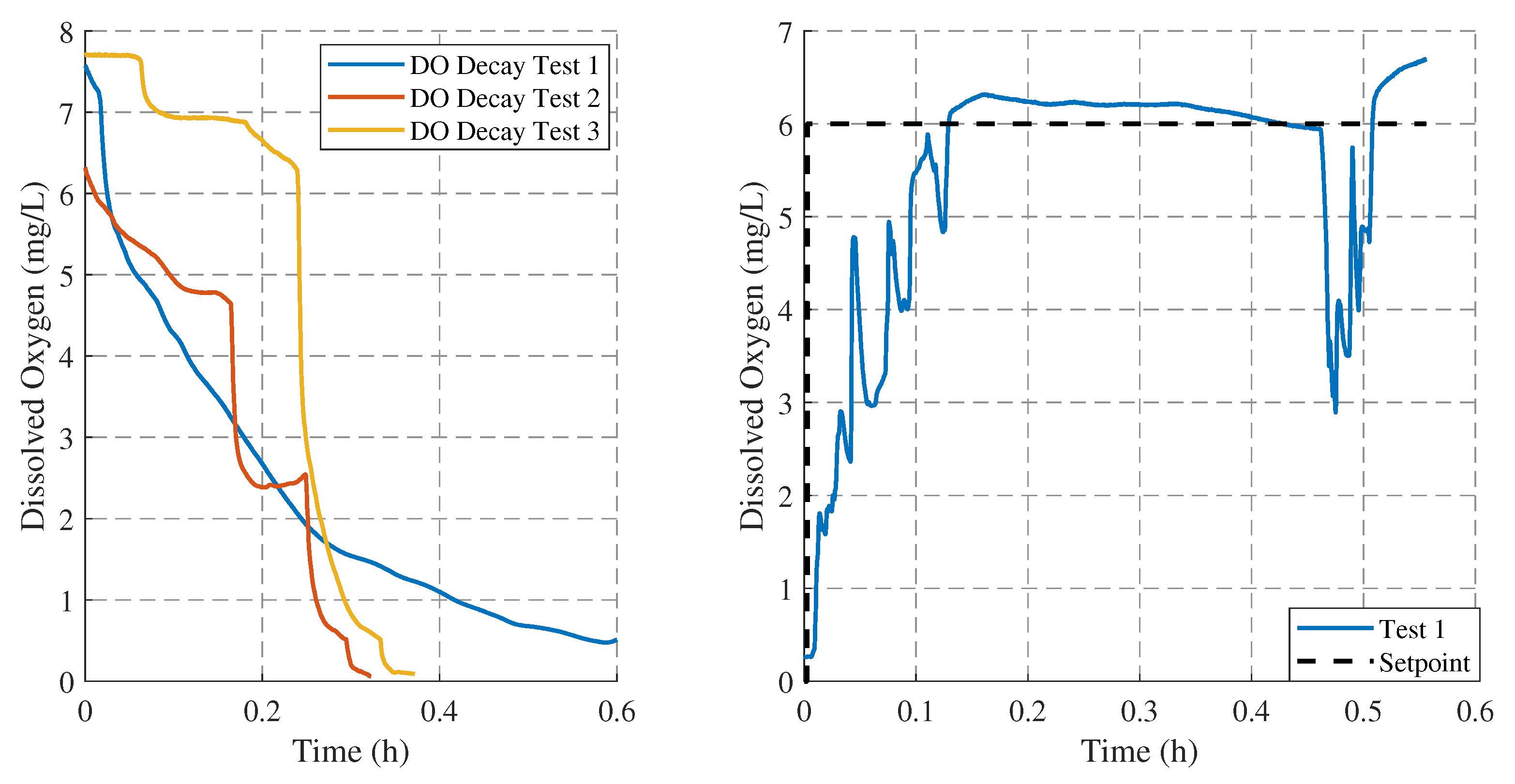
Figure 8.
Dissolved oxygen responses obtained with On–Off control over 10 repetitions at a setpoint of 6 mg/L.
Figure 8.
Dissolved oxygen responses obtained with On–Off control over 10 repetitions at a setpoint of 6 mg/L.
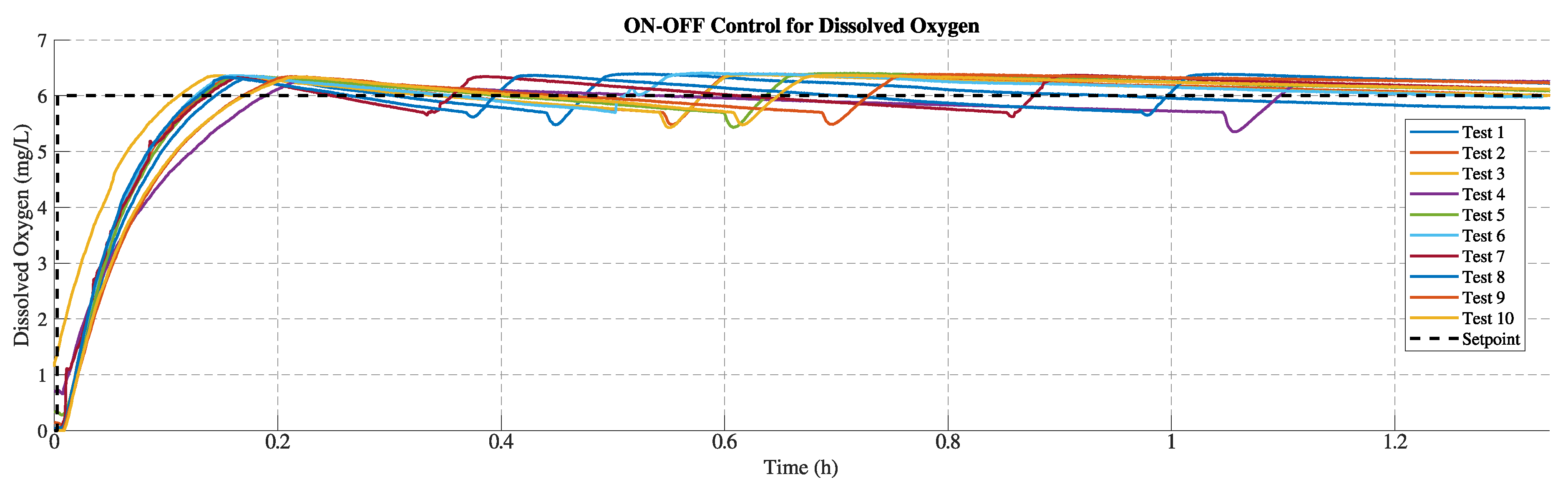
Figure 9.
Corresponding valve aperture (orange line) for Test 1 under On–Off control (blue line).
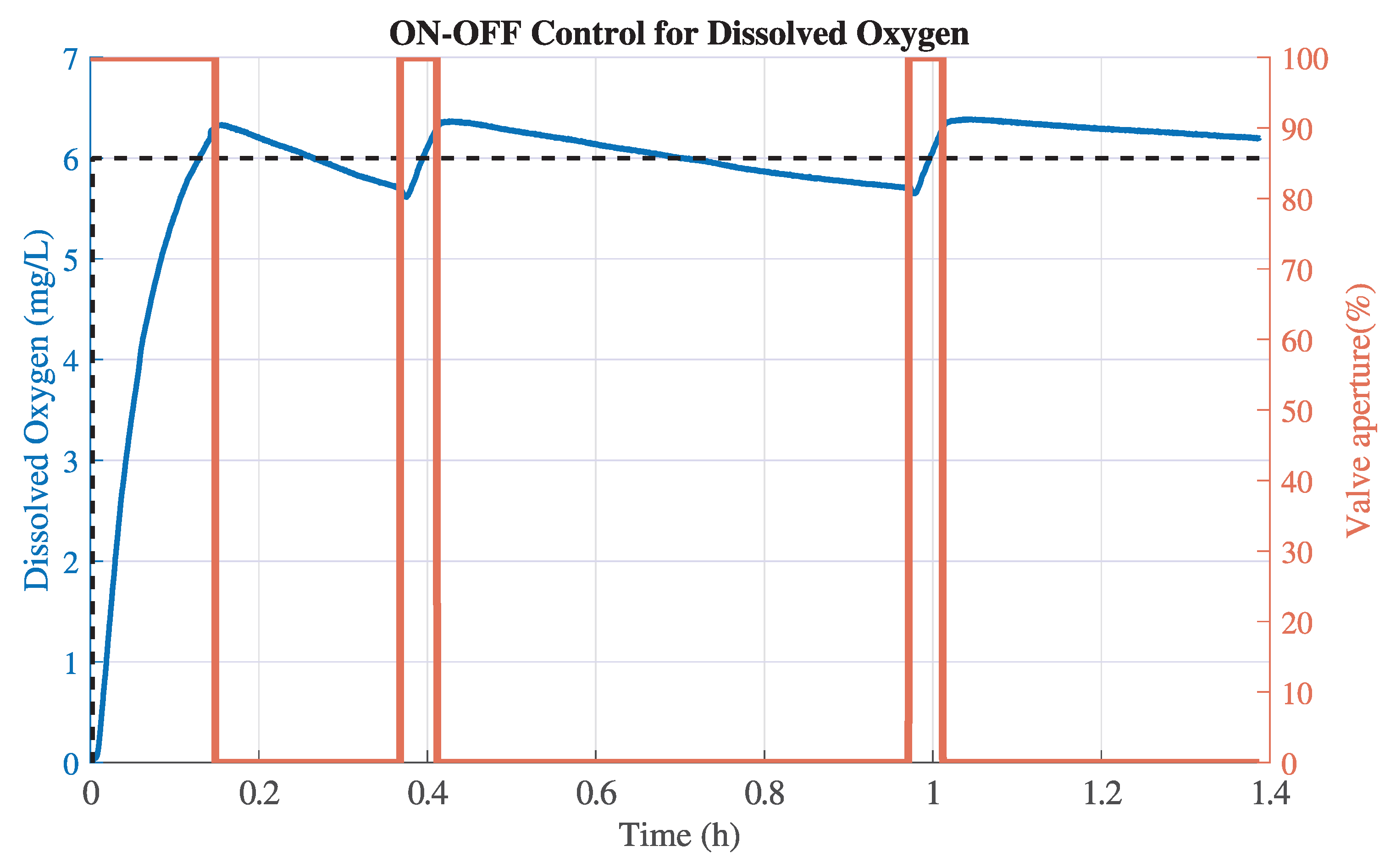
Figure 10.
Measured, filtered, and sigmoidal-adjusted reaction curves of the DO signals (gray, green, and blue lines, respectively).
Figure 10.
Measured, filtered, and sigmoidal-adjusted reaction curves of the DO signals (gray, green, and blue lines, respectively).
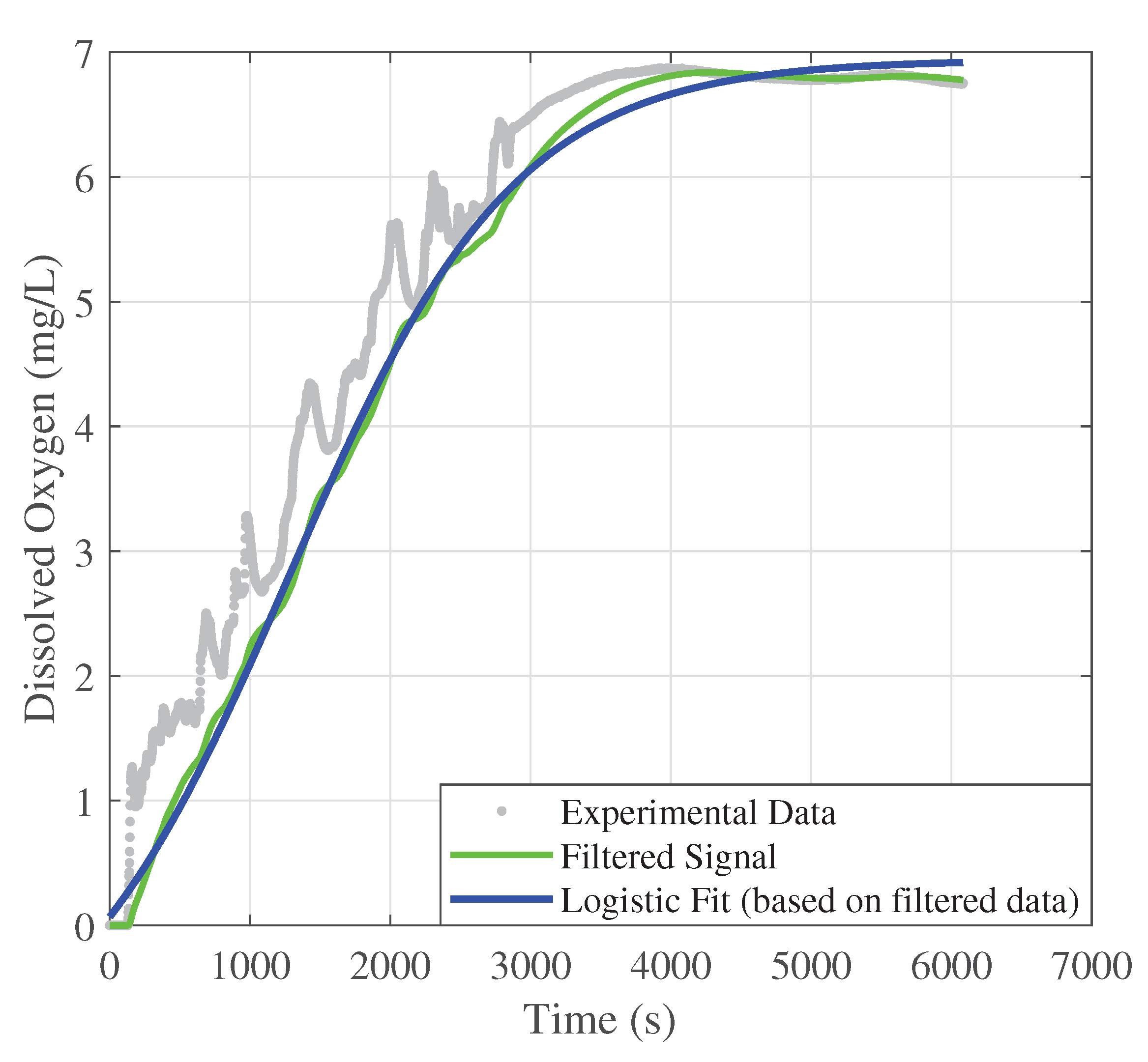
Figure 11.
Dissolved oxygen responses obtained with PID control over 10 repetitions at a setpoint of 6 mg/L.
Figure 11.
Dissolved oxygen responses obtained with PID control over 10 repetitions at a setpoint of 6 mg/L.
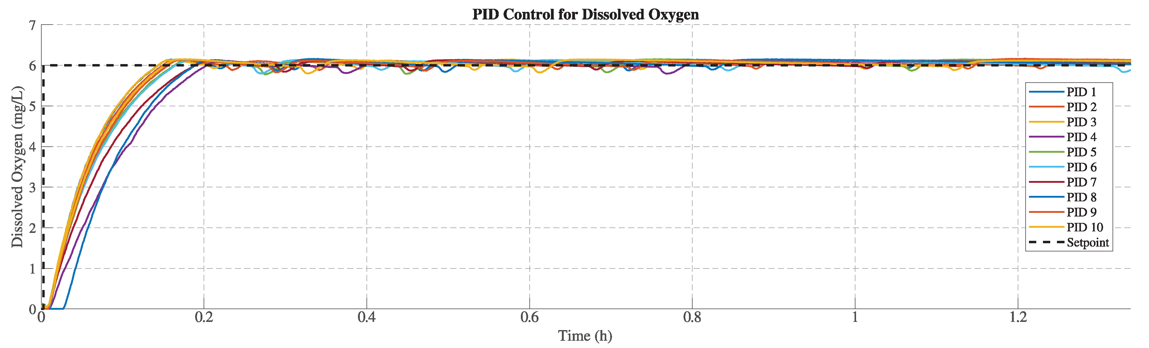
Figure 12.
Corresponding valve aperture (orange line) for Test 1 under PID control (blue line).
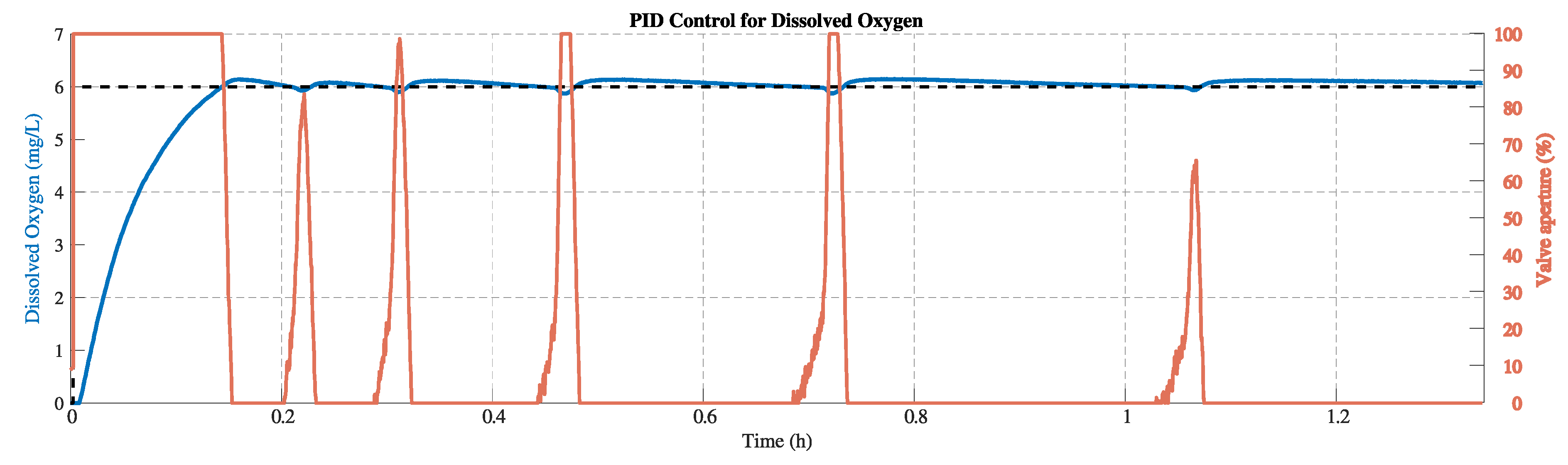
Figure 13.
Long-term effect of aeration decrease: On–Off control (left), DO control with variance shadow applied to On–Off (middle), and PID (right).
Figure 13.
Long-term effect of aeration decrease: On–Off control (left), DO control with variance shadow applied to On–Off (middle), and PID (right).
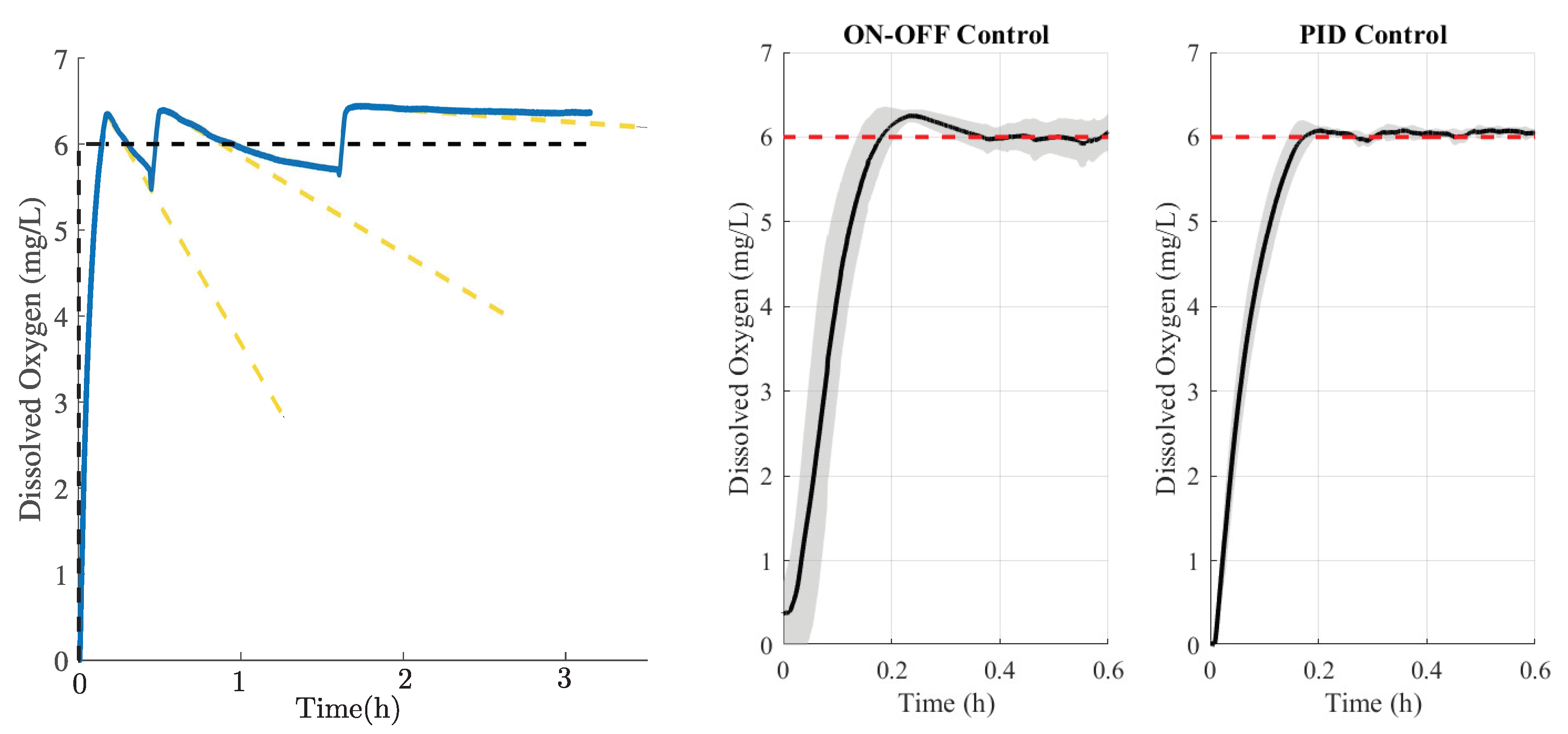

Table 1.
Main instrumentation and hardware specifications of the experimental DO control platform.
| Element | Key specifications | Function in the system |
|---|---|---|
| Process tank | Rigid tank, 160 L working volume; laboratory-scale geometry; single-phase liquid operation. | Physical process where dissolved oxygen dynamics are regulated. |
| Aerators | Submerged air diffusers; porous stone type; characteristic pore size in the sub-millimeter range; installed symmetrically at the tank bottom; nominal airflow ≈1–3 L/min per aerator. | Promote gas-liquid oxygen transfer and spatially uniform aeration. |
| Air compressor | Oil-free air compressor; Set to a pressure of 3.5 bar; air tank capacity ≈40 L; nominal flow capacity ≈160 L/min. | Provides pressurized air to the aeration subsystem. |
| Flow control valve (FV1) | Proportional valve; 2-way normally closed; maximum flow up to ≈60 SLPM; operating pressure up to 3.5 bar; current-driven actuation (0–175 mA). | Final control element regulating aeration rate. |
| Valve driver | Analog current driver; PLC-compatible input; valve supply voltage 12–14 VDC; maximum output current ≈200 mA. | Conditions the PLC output to drive the proportional valve. |
| DO sensor | Optical dissolved oxygen probe; measurement range 0–20 mg/L; accuracy ±0.1 mg/L; Modbus RS-485 communication; integrated temperature compensation. | Provides real-time DO measurements for feedback control. |
| Controller | Programmable Logic Controller (PLC); discrete-time execution; analog output (4–20 mA); serial communication via RS-485 (Modbus). | Executes the closed-loop DO control algorithm. |
| DC power conversion | DC-DC converters; 24 VDC main supply stepped down to 12 VDC and 14 VDC; current capacity up to 3 A. | Supplies regulated power to valve driver and instrumentation. |
Table 2.
Test results and average performance of the On-Off Control
| Test | Overshoot () | Rising time (s) | Settling time (s) | (mg/L) |
|---|---|---|---|---|
| 1 | 44.4 | 346.5 | 454.0 | 36.0 |
| 2 | 46.2 | 313.5 | 412.5 | 25.2 |
| 3 | 37.8 | 291.0 | 339.0 | 9.6 |
| 4 | 34.2 | 523.5 | 595.0 | 21.0 |
| 5 | 93.6 | 326.5 | 425.5 | 51.6 |
| 6 | 71.4 | 303.0 | 400.5 | 28.8 |
| 7 | 37.2 | 339.5 | 426.0 | 10.8 |
| 8 | 38.4 | 301.5 | 402.0 | 22.2 |
| 9 | 38.4 | 406.5 | 529.5 | 9.6 |
| 10 | 36.6 | 402.0 | 530.0 | 2.4 |
| Average | 47.4 | 355.4 | 451.4 | 21.6 |
Table 3.
Test results and average performance of the PID Control
| Test | Overshoot ( mg/L) | Rising time (s) | Settling time (s) | (mg/L) |
|---|---|---|---|---|
| 1 | 15.0 | 340.5 | 449.0 | 4.2 |
| 2 | 13.8 | 355.5 | 468.5 | 6.6 |
| 3 | 13.8 | 338.5 | 446.5 | 6.0 |
| 4 | 12.0 | 505.0 | 651.0 | 10.8 |
| 5 | 42.6 | 396.5 | 514.0 | 6.6 |
| 6 | 15.6 | 399.0 | 519.0 | 6.0 |
| 7 | 12.6 | 459.5 | 590.0 | 9.0 |
| 8 | 15.6 | 412.5 | 606.0 | 10.2 |
| 9 | 16.2 | 372.5 | 493.0 | 3.6 |
| 10 | 20.4 | 363.5 | 477.5 | 6.0 |
| Average | 17.4 | 394.3 | 521.5 | 7.2 |
Table 4.
Summary of required repetitions and statistical indicators for each controller (95% confidence interval).
Table 4.
Summary of required repetitions and statistical indicators for each controller (95% confidence interval).
| Controller | Rel. Error (%) | Rel. (%) | ||||
|---|---|---|---|---|---|---|
| On-Off | 8 | 0.2565 | 0.0482 | 0.1140 | 4.28 | |
| PID | 3 | 0.0560 | 0.0072 | 0.0310 | 0.93 |
Disclaimer/Publisher’s Note: The statements, opinions and data contained in all publications are solely those of the individual author(s) and contributor(s) and not of MDPI and/or the editor(s). MDPI and/or the editor(s) disclaim responsibility for any injury to people or property resulting from any ideas, methods, instructions or products referred to in the content. |
© 2026 by the authors. Licensee MDPI, Basel, Switzerland. This article is an open access article distributed under the terms and conditions of the Creative Commons Attribution (CC BY) license (http://creativecommons.org/licenses/by/4.0/).
Copyright: This open access article is published under a Creative Commons CC BY 4.0 license, which permit the free download, distribution, and reuse, provided that the author and preprint are cited in any reuse.


