Submitted:
25 February 2026
Posted:
26 February 2026
You are already at the latest version
Abstract
This study examines the relationship between house prices and the factors driving their growth under conditions of transition from a long-standing currency board regime to Eurozone membership. The main objective is to identify and quantify key factors explaining the variation in house price growth in Bulgaria in conditions of prolonged currency convergence. The study applies a set of econometric techniques, including stationarity tests (ADF), Ljung-Box estimation, Shapiro-Wilk test, Kolmogorov-Smirnov test, ARCH LM test, t-tests. The study is based on 40 observations of quarterly data for the period 2015Q4-2025Q3 on 48 selected predictors with an impact on the general house price index. The final ARIMAX(0,2,1) model contains estimates of second-differenced data. The model includes a first-order moving average component and three exogenous regressors: the homeowners' expense index, the average rents of housing in Bulgaria and the homeowners' utility expenses index. The model explains nearly 90% of the variation in the acceleration of housing prices, with a low mean squared error. The diagnostic analysis confirms the adequacy of the model with a lack of autocorrelation in the residuals and successful capture of all systematic information in the data. All three exogenous regressors are statistically significant at the 1% level with strong and stable impacts on the dynamics of housing prices. The non-parametric correlation analysis shows statistically significant monotonic relationships between all regressors and the dependent variable. For the set of traditional macroeconomic, demographic, financial and industry factors, no statistically significant relationship is established. The results show that during Bulgaria's transition from a currency board to the Eurozone, the sustainable growth of housing prices was due to factors of national specificity.
Keywords:
house prices
; ARIMAX
; Eurozone
; Bulgaria
; ADF
; Ljung-Box
; Shapiro-Wilk тест
; Kolmogorov-Smirnov тест
; ARCH LM
1. Introduction
Bulgaria’s accession to the Eurozone on 1 January 2026 completes a long process of currency convergence that began with the introduction of the currency board in 1997. This historical moment puts the country in a unique position to study the effects of currency integration on the housing market – a position that combines the characteristics of a small open economy with almost three decades of fixed exchange rates to the German mark and the euro. While the literature presents numerous analyses of housing markets (Pagourtzi, Assimakopoulos, Hatzichristos, & French, 2003) in established Eurozone members and separate studies of the post-communist transformation of real estate in Eastern Europe, there is a significant gap in understanding how housing prices are formed at the moment of a currency transition from a long-term currency board to Eurozone membership.
Existing research on real estate prices in Central and Eastern European countries (Marinković, Džunić, & Marjanović, 2024), (Idirizov, 2025) typically focuses either on the period of post-communist privatization and liberalization (Egert & Mihaljek, 2007), or on the effects of EU accession (Ciarlone, 2015), or - for the few countries that adopted the euro - on the consequences of monetary integration (Dandashly & Verdun, 2021). What is lacking is a systematic analysis of a wide range of determinants of housing prices in the context of a long-term monetary convergence that preceded formal membership. Bulgaria presents a unique case for such an analysis. Unlike countries such as Slovakia, Estonia or Lithuania, which adopted the euro after relatively short periods of preparation, Bulgaria maintained a fixed exchange rate to the euro (initially by pegging it to the German mark since 1997) for nearly thirty years before entering the Eurozone. This long transitional state creates a specific institutional environment in which expectations of currency stability are already ex ante materialized, but the institutional mechanisms of the monetary union are not yet operational. The question arises whether, in such a configuration, housing prices move according to determinants characteristic of economies in transition, of countries in the process of convergence, or already reflect dynamics typical of Eurozone members. Secondly, the question of the impact of accession expectations, which would form an anticipatory increase in the house price index (Liu, Farahani, & Serota, 2024), in which fundamental factors such as GDP and wages would turn out to be lagging behind price growth. Thirdly, the question of the possible independent trajectory of house price dynamics, based on the processes of cohesion of household wealth in the EU member states as a whole and the Eurozone in particular, is raised. The search for answers to these questions points to the problematic area of the study.
The problem area of this study focuses on the identification of the key factors that drive the growth of house prices in Bulgaria during the decade 2015-2025 - a period that covers both the phase of intensive preparation for Eurozone membership and the pandemic shock with a strong negative effect on the population for Bulgaria, followed by the approval of admission to the Eurozone with the published convergence report on 4.6.2025 (European Commission, 2025). From a theoretical point of view, this period represents a natural experiment for studying the stability of determinants under changing institutional regimes. From a practical perspective, understanding these factors (Yordanova & Hristozov, 2025) has direct effects for the implementation of macroprudential policy and the monitoring of financial stability in the conditions of a new exchange rate regime with the introduction of a new currency (Atanassov, Trifonova, Saraivanova, & Pramatarov, 2017).
The central research gap that this study addresses is the lack of empirical models that systematically test which of the many potential determinants of house prices retain explanatory power under conditions of continued currency convergence. While studies of housing markets in individual Eastern European countries exist, they rarely use a stepwise approach to select factors from a wide range of variables and even less often cover the period immediately before and during Eurozone accession. This methodological gap is particularly problematic because it limits the ability of policymakers and central bankers to identify which indicators are truly benchmarks for monitoring the housing market under changing institutional conditions. Eurozone accession is a psychological factor with a powerful influence on buyers and sellers of residential properties (Visković & Čipčić, 2025). Comparisons between property prices before and after accession to the Eurozone are in favor of the accession effect, which supports the convergence process, including in terms of household wealth growth.
The aim of the study is to identify and quantify the key factors that explain the dynamics and growth rate of the variation in house prices in Bulgaria during the period 2015-2025 in conditions of prolonged currency convergence, using a methodological approach for selection from a wide range of macroeconomic, financial, demographic and sectoral variables.
To achieve this goal, the following research tasks are formulated: 1) to construct an extensive set of potential explanatory variables/predictors, covering all the main channels of impact on housing prices identified in the literature and form their grouping; 2) to apply a pre-selection procedure within the groups of factors with the selection of representative predictors suitable for subsequent econometric processing; 3) to select statistically significant predictors based on the requirements for data stationarity; 4) to assess the stability of the identified factors in different sub-periods; 5) interpret the results in the context of the positive report on achieving convergence in 2025Q2 with the announcement of 1.1.2026 as the date for joining the Eurozone, which fundamentally changes the country's status as the 21st member state of the Euro Area.
The preliminary analysis allows us to accept the existence of several objective limitations to this study. First, the analysis uses quarterly data for a ten-year period (2015-2025), which provides 40 observations - sufficient for a statistically valid assessment, but conservative in terms of assessing high-frequency dynamics in factors with daily, weekly or monthly generated market price data. Second, the focus is on national aggregated data, which conceals regional differences in housing markets, where capitals usually have a leading influence on national trends. Third, the econometric procedure is effective for selecting statistically significant variables, but for methodological reasons (autocorrelation, non-stationarity of data, etc.) it requires de-selection of predictors in the final model. However, these predictors, according to financial-economic logic, have an impact on the general housing price index (GHPI), based on the objective cause-effect relationship. Fourth, the observation period includes only a short period of accumulation of the effect of the publication of the convergence report on Bulgaria's accession to the Eurozone on 1.1.2026, which limits the possibilities for assessing the long-term effects of currency integration.
On this basis, the research has the following content structure. After this introduction with justification of the relevance, research gap, goal, objectives and constraints, section two presents an analytical overview of contemporary research on the determinants of housing prices with justification of their possible grouping. Section three consistently focuses attention on international trends in the EU household housing sector, the collection of national data with predictors and their grouping, the development of a methodological approach and the procedure for their subsequent validation based on correlations with the dependent variable GHPI. Section four presents the results of the analysis, including the statistical characteristics of the final model and the estimates of the individual factors. Section five discusses the interpretation of the conclusions in light of theoretical expectations, the institutional context and empirical evidence for other national residential real estate markets. Section six summarizes the main conclusions, outlines areas for application of the results within the scope of institutional policy justification, and suggests directions for future research.
2. Literature Review and Hypotheses
In the scientific literature, the issue of housing price dynamics has a lot of evidence of studies on the determinants of dynamics and growth at regional, national, continental and global levels. A characteristic feature of these studies is the derivation of the influence of macro factors as the basis of models for assessing the dynamics and growth of housing prices. In this group, the focus on GDP and/or its components (Algieri, 2013) finds a number of confirmations of its influence on housing prices. The focus of these studies provides evidence for the influence of GDP as a universal fundamental factor (Li & Zeng, 2010), both in a number of national studies (Cohen & Karpavičiūtė, 2017), (Ubarevičienė & Aidukaitė, 2026), (Mazáček & Panoš, 2025), and studies at the level of leading urban agglomerations (Sivitanides, 2018), (Reichle, Fidrmuc, & Reck, 2023), where the focus is on the problem of housing affordability in capital cities (Haandrikman, Costa, Malmberg, Rogne, & Sleutjes, 2023), regional differences (Prodanov & Naydenov, 2020), (Sabitova, Shavaleyeva, Lizunova, Khairullova, & Zahariev, 2020) and the objective growth of prices justified by supply deficits (Stroebel & Vavra, 2019). At the macroeconomic level, inflation is also a subject of research (Anari & Kolari, 2002) as a fundamental factor influencing housing prices (Kuang & Liu, 2015), (Cohen & Karpavičiūtė, 2017).
The second group of factors can be considered as services for acquisition, maintenance (Gurmu, Krezel, & Ongkowijoyo, 2021) and repair of (Taggart, Koskela, & Rooke, 2014), (Park & Seo, 2024), which also have their objective impact on housing prices. The acceptance standards for new construction in Bulgaria are at the "internal linings and plastering" stage, after which the services for finishing the housing to living standards, including furnishing, require additional funds. The situation is no different when purchasing an existing property (Passek & Nübel, 2025), where the new owner returns to the specified stage and changes the interior of the newly purchased property, paying for services for major repairs of the housing (Aydinli, 2024).
Third, the factors of energy provision and utility services of housing by households should be assessed, which have a sustainable trend of increasing volatility in conditions of multiple crises (Ushenko, et al., 2023). Home ownership faces the burden of increasing energy costs (Shen, Li, Zhu, Liu, & Luo, 2022), (Cermáková & Hromada, 2022), utilities (Mazáček & Panoš, 2025), housing rental costs (Doling & Ronald, 2010) and taxes (Iliopoulou, Krassanakis, & Kappelos, 2025). Among these costs, investments to improve the energy efficiency (Zhelyazkova, 2018) of owned homes should also be taken into account (Ciot, 2022). Next, as a fourth group, we estimate the impact of the number of new buildings and dwellings built with a corresponding number of rooms. Design costs and construction materials (Herrera, Sánchez, Castañeda, & Porras, 2020), (Zhang, Wang, Xu, Yang, & Meng, 2024), with the subsequent supply of newly built dwellings (Araya, et al., 2024), (Pazdzior, Sokol, & Styk, 2021), (Caldera Sánchez & Johansson, 2011) are determinants of pricing (Mayer & Somerville, 2000), incl. when taking into account the effects of the COVID-19 pandemic on safety measures in the working conditions of construction workers (Ebekozien & Aigbedion, 2021).
The fifth group of factors focuses on housing-seeking families with their incomes (Ünalan, Çamalan, & Yılmaz, 2025) and employment. The income (McQuinn & O'Reilly, 2008) and the labor market with employment and unemployment indicators (Irandoust, 2019) are an objective group of indicators influencing housing demand, which have been evaluated in a number of studies (Girouard, Kennedy, Noord, & André, 2006). In sixth place we place the credit conditions for purchasing housing. Financing housing purchases and mortgage interest rates (McQuinn & O'Reilly, 2008), (Lin, Lee, & Newell, 2022) are major factors, widely covered in the literature (Girouard, Kennedy, Noord, & André, 2006). In the final seventh place we place overseas investments in housing on the national market and the alternative for wealth growth through stock market trading in securities. Home ownership is part of household wealth and the rational management of this wealth should take into account investment alternatives (Ouhinou, et al., 2025), the stock market (Zaharieva, Tarakchiyan, & Zahariev, 2022) and foreign currency-denominated assets, which factors also have the potential to impact housing prices.
Based on the literature review presented above and the derivation of seven groups of factors influencing housing prices, the research hypothesis is formulated that, regardless of institutional changes and external shocks, the variation in housing prices in Bulgaria is explained by a limited number of predictors, with the sustainability of the impact based on the long-term pegging of Bulgaria's national currency to the euro through the currency board and the demand for housing by households at prices that are expected to accumulate growth due to the prospect of admission to the Eurozone.
3. Materials and Methods
3.1. General Data Collection and Interpretation
The EU27 Member States are an example of the uniqueness of national characteristics compared to the community average in terms of household home ownership. On average for the EU27 in 2024, 31.6% of the population lived in rented housing, while 68.4% of the population owned their own home (Eurostat, 2025a). The gap in the EU27 indicator in terms of the place of residence of households is 47.1% between the country with the lowest and the country with the highest level of rental housing. The first quartile of the highest share of ownership is Romania with 94.3%, followed by Slovakia, Hungary, Croatia, Lithuania, Poland and Bulgaria. In contrast, Germany is the only country where the share of households living in their own homes is below 50%, compared to 52.8% of households living in rented housing (See Figure 1).
The data suggest the importance of national research in the scope of housing investment, which would reveal specific national factors and influencing predictors of GHPI growth, which logically would not have universal application for all EU27 countries. The balance between renting and owning a home is a function of their affordability, measured by the price of the home and the cost of renting it. In both cases, the choice can be methodologically supported by appropriate financial analysis tools (Nenkov & Hristozov, 2022). According to the latest estimates of the European Parliament, a sustainable trend of increasing house prices and rents is observed in the European Union, reaching a “crisis situation” level (European Parliament, 2025). The data indicate an average increase in house prices in the EU27 of 53.44% for the period 2015-2024, with Hungary leading the way with a house price increase, measured by the GHPI of 209.86%, followed in the first quartile by countries with the highest house price growth rates in Lithuania, Portugal, Czechia, Bulgaria, Estonia and Poland. At the other end of the scale in terms of the HPI change rate is Finland, with a GHPI increase of only 1.35% over a 10-year period (Eurostat, 2026a).
Regarding the amount of rents in the EU for residential purposes, there is a lag in the average growth rates compared to those in housing prices. Based on 2010, in the period up to 2024, the increase in housing rents in the EU is 25%. The largest increase in housing rents is reported in Estonia (+208%), followed by Lithuania (+177%), Ireland (+108%) and Hungary (+107%), while in Greece a decrease in rents of -16% is reported (Eurostat, 2025a). The data and trends illustrated by graphs allow us to conclude that there is strong national diversity among EU member states in terms of housing prices, represented by the GHPI. Among these countries, with its accession to the Schengen area in early 2025 and to the Eurozone from 01.01.2026, the example of Bulgaria stands out (See Figure 2), where the increase in the housing price index for the period 2015-2024 exceeds the EU average levels by 2.2 times, and the average annual growth rate of the GHPI for Bulgaria exceeds that of the EU27 for the same period by 1.82 times.
On this basis, it is of scientific interest to select the factors that push up the GHPI in Bulgaria with a focus on the period 2015 - 2024 with a base of 2015=100. The indicated data also correspond to the increase in 2024 compared to 2015 of Bulgaria's GDP per capita by 2.48 times (Eurostat, 2025b), and of GDP at current prices in billion euros by 2.37 times. The indicated results were achieved in conditions of macroeconomic equilibrium with sustainable compliance with the Maastricht criteria for membership in the Eurozone and HICP for 2024 of 2.6%.
3.2. Research Data Collection, Grouping and Preselection
For the purposes of this study, data were collected on 48 factors (See Appendix A.1) that have a logical connection with the pricing of housing in Bulgaria, both at the construction stage and at the stage of repairs, maintenance and utility operation. From a market perspective, indicators of the supply of new housing are represented, such as data on the construction of buildings and housing by groups (from one-room to those with six or more rooms). On the demand side, financial and economic factors providing funds for purchase were studied, through wages, loans, mortgage interest rates, as well as the alternative growth rate of wealth, expressed through the stock exchange index (Gönül & Omay, 2025). When evaluating the historical data for 43 of the studied predictors, a net increase is established for the period 2015Q4 to 2025Q3, and for 5 predictors - a decrease.
The dependent variable is represented by the general housing price index, which for the period of 10 years increased by 2.56 times, compared to the GDP growth, where the increase was 2.75 times and the growth of wages with an increase of 2.86 times. The sub-indices of old housing (HPIEH) and new housing (HPINH) report growth of 2.75 and 2.32 times, respectively. For the studied period, the working-age population of Bulgaria decreased by 7.89%. In terms of financial indicators, the most significant is the decrease in the predictor "Bad and restructured housing loans" by 86.7%, followed by the BNB interest rate with a decrease of 58.08% and the mortgage interest rate with a decrease of 57.92%. The unemployment rate also decreased by 56.96% and reached the second lowest level in the EU (Eurostat, 2026c) of 3.3% as of the date of the country's accession to the Eurozone on 1.1.2026.
Econometric modeling of the database revealed that the lowest coefficient of variation among all 48 predictors is 15 predictors with a variation of up to 20% compared to the average for the period, 16 predictors with a variation of 20% to 30%, 12 predictors with a variation of 30% to 40%, and the remaining 8 predictors with a variation of over 40%, with the highest indicator being recorded for the construction of new homes with 6 or more rooms, where the coefficient of variation reaches 59.13%. The results with selected indicators from descriptive statistics and the dynamics of the factors by quarters for the historical data against the GHPI are presented in Appendix A.2. Graphical evidence of the dynamics of the data at first differentiated for traditional macroeconomic, financial, demographic and sectoral factors is presented in Appendix A.3.
3.3. Empirical Methodology and Model Specification
3.3.1. Methodology
In the literature, housing price estimation is a challenging area, where evidence is found for a variety of methods Housing price estimation methods can be grouped as traditional and advanced. Traditional methods include regression models (Yan, 2024) comparison-based models, production cost models, income flow models, housing investment return models, etc. Advanced methods include artificial neural networks (Mimis, Rovolis, & Stamou, 2013), spatial analysis methods, hedonic pricing methods, fuzzy logic methods, and ARIMA (Pagourtzi, Assimakopoulos, Hatzichristos, & French, 2003). The latter method solves a number of methodological problems by allowing the integration of the influence of past data with estimates of their autocorrelation and trend, with the derivation of models with statistically significant predictive power.
To analyze the dynamics of the household housing price index, an ARIMA model (Kotu & Deshpande, 2019) with exogenous variables (ARIMAX) is constructed by applying a multi-step approach to determining the determinants and assessing their influence. First, the data are checked for stationarity using the extended Dickey-Fuller test (Dickey & Fuller, 1981). This test is based on two hypotheses. The null hypothesis states that the time series has a unit root, i.e. the series is non-stationary, and the alternative hypothesis is that there is no unit root and the series is stationary. To confirm the presence of stationarity, the p-value obtained from the ADF test must be lower than 0.05. The variables are sequentially differentiated until the series are stationary (Distaso, 2008). Second, for the exact specification of the model using the Kruskal–Wallis test, the dependent variable is checked for seasonality. The null hypothesis states that there are no statistically significant differences between the groups (there is seasonality), and the alternative that there is at least one group that is statistically significantly different from the others. The null hypothesis is rejected if p-value < 0.05. It is suitable for small samples, such as ours, because it does not require a normal distribution of observations. Fourth, final specification of the model based on the tests conducted and stepwise elimination of variables based on their statistical significance. Fifth, analysis of the results is performed. Sixth, diagnostic tests for autocorrelation of the residuals, normality and ARCH effects are performed. The main data processing is performed with IBM SPSS Statistics 27, and for the ADF test, the adf.test() function from the tseries package with R 4.4.3 is used.
3.3.2. Stationarity and Seasonality Tests
The Augmented Dickey-Fuller test of the original data of the dependent variable does not confirm the presence of stationarity (Sen, 2008), since the p-value > 0.05 (p = 0.99) and therefore the null hypothesis cannot be rejected. After the first difference also turned out to be non-stationary (p-value = 0.5984) (See Appendix B.1), a second differencing of the dependent and independent variables in the model is applied. The stationarity check after the second differencing shows that six out of 48 variables are still non-stationary (HICP, MMRD, SMRD, OSRD, FHERHM and BLSRP), which is why they are excluded from further analysis. For all other variables, including the dependent one, the p-value < 0.05, which confirms the achievement of stationarity of the time series.
After achieving stationarity, the data are tested for the presence of seasonality. For this purpose, the non-parametric Kruskal–Wallis test is applied. Its results (H = 0.353; p = 0.950) do not indicate statistically significant differences between the neighborhoods, i.e. the presence of seasonality. Therefore, it is not necessary to include a seasonal specification in the ARIMAX model (See Table 1).
3.3.3. Model Specification
The final specification of the model is achieved by sequentially excluding the factors initially included in the model by comparing two variants: with and without a constant. The data obtained show that the inclusion of the constant in the model worsens its characteristics, and the coefficient of the constant has no statistical significance at a 95% confidence interval (β = 0.031, p-value = 0.653). Removing it improves the characteristics of the model (RMSE, MAPE, BIC and Ljung-Box Q). Finally, an ARIMAX(0,2,1) model is reached without a constant and with three exogenous variables (OOHE, WSMSRD and ARH). Formally, the model can be represented as follows (See Formula 1):
where:
is the second difference of the dependent variable at time t;
– the second difference of the ith independent variable at time t;
– the regression coefficient for the corresponding independent variable;
– first-order MA coefficient;
– stochastic error at time t;
– stochastic error from the previous period.
The specific specification of the model (See Formula 2) is as follows:
where:
means second difference;
– General Haus Price Index;
OOHE - Owner-Occupiers Housing Expenditures;
ARH – Average Rent of Housing;
WSMSRD – Water Supply and Miscellaneous Services Relating to the Dwelling;
– the coefficient of the MA(1) component;
, – the coefficients of exogenous variables;
– stochastic error;
– stochastic error from the previous period.
4. Results
4.1. Model Fit
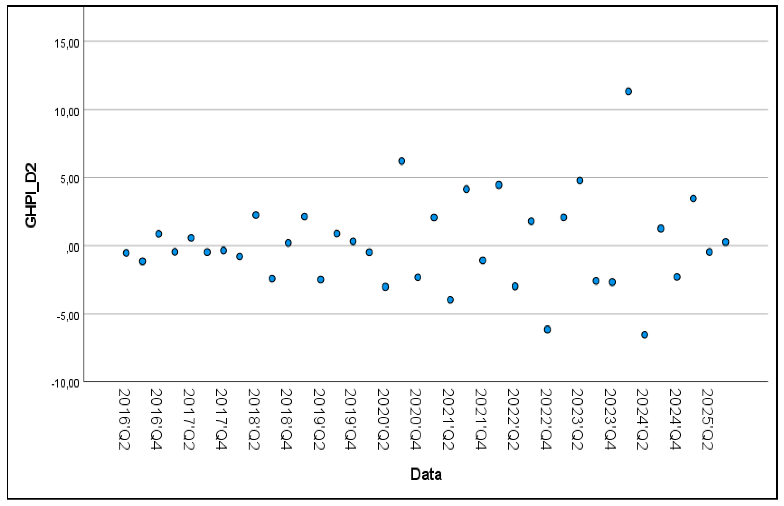
The model is estimated on the basis of pre-differentiated data, which is why the description table is listed as ARIMA(0,0,1)(0,0,0), and the variables as GHPI_D2, OOHE_D2, WSMSRD_D2, and ARH_D2 (see Table 2). Stationary R-squared, RMSE, MAE, and Ljung-Box Q test are used for its estimation. The plot of the distribution of the second-differentiated values of GHPI over time illustrates that the values vary in a relatively narrow range (approximately from -6.53 to +11.34), with a significant part of the observations concentrated around zero (See Figure 2). At such values, even minimal absolute errors lead to extremely high percentage deviations, which makes MAPE a mathematically inappropriate metric for model estimation (Hyndman & Koehler, 2006).
The stationary R-squared is 0.873, indicating that the model explains 87.3% of the variation in the second differences of the GHPI. This means that 87.3% of the changes in the acceleration/deceleration of house price growth are explained by changes in the differenced values of the independent variables (OOHE, WSMSRD and ARH). The remaining 12.7% is due to other factors not included in the model.
Figure 3.
Scatter Plot of GHPI_D2 by Data.
The mean absolute error (MAE) is 0.902 units, and the root mean square error (RMSE), is 1.252, see Table 3. The ratio MAE/SD = 0.268 indicates that the mean absolute error represents 26.8% of the standard deviation of the stationary series, which is considered a very good relative forecast accuracy. The ratio RMSE/MAE = 1.39 indicates that the errors are relatively evenly distributed without extreme deviations. The Ljung-Box Q test (See Table 4) confirms the lack of autocorrelation in the residuals (Q(18) = 11.785, p = 0.813).
4.2. Parameter Estimation
The data from the ARIMA model parameter table show that the coefficients of the independent factors and MA are positive and statistically significant at the 1% significance level (See Table 5). The coefficient β1= 0.624 (p-value < 0.001) shows that an increase in the acceleration/deceleration of Owner-Occupiers Housing Expenditures by one unit leads to an increase/deceleration of the acceleration of GHPI by approximately 0.63 units. The coefficient β2=0.171 (p-value < 0.01) shows that an increase in the acceleration/deceleration of the independent Water Supply and Miscellaneous Services Relating to the Dwelling by one unit leads to an increase/deceleration of the acceleration of GHPI by approximately 0.17 units. The coefficient β3=0.421 (p-value < 0.01) shows that an increase in the acceleration/deceleration of the independent Average Rent of Housing by one unit leads to an increase/deceleration of the acceleration of the GHPI by approximately 0.421 units. The significant first-order Moving Average component (θ₁ = 0.693, p < 0.001) shows that shocks to housing prices have a persistent effect. An unexpected change in prices in one quarter has an impact of 69.3% on the change in the next quarter. This suggests the presence of inertia in price dynamics. Since |θ₁| < 1 the model is reversible and allows for reliable forecasts.
To determine the individual contribution of each variable, standardized coefficients were calculated, with OOHE β_std being 0.79, ARH β_std being 0.26, and WSMSRD β_std being 0.26. This means that for an equal change of one standard deviation, OOHE has the strongest effect on changes in house prices, while the other two factors have similar contributions. The indicators of the descriptive statistics of the dependent and independent variables confirm the robust parameters of the studied factors (See Appendix B.2).
4.3. Financial and Economic Evaluation of ARIMAX Results (0,2,1)
The economic interpretation of the three factors should reflect the specificity of the Bulgarian housing market, where the net change in the subindex of existing housing is 2.715, while the net change in the subindex of newly built housing is only 2.322 over the ten-year period. This initial observation clearly shows the importance of the costs associated with existing housing in their specificity and complexity as pricing factors on the general index – GHPI.
The first factor in the ARIMAX (0,2,1) model, Owner-Occupiers Housing Expenditures is a synthetic index (2015Q4=100), which aggregates various expenses of homeowners, both for the acquisition itself, including notary, agency and administrative costs upon acquisition, as well as expenses of a current nature (taxes) and those for major repairs and maintenance, supplemented by all other not-classified property costs. Key to understanding the significance of the factor is the significant difference in the standards of completion when buying a newly built home in Bulgaria and an existing home. While with existing homes the buyer can move in and live directly, with newly built homes the costs to reach the living stage can reach up to 50% of the price paid, which includes significant in scale and time finishing works and furnishing, which varies according to the quality of the furniture and electrical equipment. The economic mechanism is demand-pull: OOHE covers the full life cycle of the owner's expenses - from acquisition to ongoing maintenance. The acceleration in these costs directly reflects the increasing willingness to pay in the market and is immediately transmitted to the general price index. In addition to the costs of the acquisition itself, incl. agent, notary and local taxes for the acquisition of the property, all maintenance and ownership costs are added here, which add a cost-push dimension: the increase in the cost of repairs and finishing works increases the full cost of residential use and is capitalized in the market value of the properties. These costs, in addition to the materials used, also include the labor costs of the workers who bring the housing ready for occupancy and living. The contribution of the factor can be expressed as follows: Contribution OOHE,GHPI =0.624⋅Δ2OOHEt.
The second factor, in the Average Rent of Housing model, has a lower β-coefficient value. The average rent functions as an arbitrage mechanism between the rental and purchase-sale segments of the housing market. The relationship follows the logic of the capitalization model (See Formula 3).
where:
Pt = ARHt/(rt – gt),
rt is the discount rate;
gt – the expected growth in rents.
The acceleration of rents Δ2ARHt > 0 acts through two channels simultaneously: first, rational tenants switch to buying (substitution effect), increasing demand; second, investors revalue the profitability of housing assets upwards, which increases prices in the sales market. ARH is both a signal of supply deficit and a measure of investment attractiveness of housing. The contribution of the factor can be expressed as follows: Contribution ARH,GHPI = 0.421. Δ2ARH. The third factor, Water Supply and Miscellaneous Services Relating to the Dwelling is a synthetic index (based on 2015Q4=100), aggregating four components of mandatory infrastructure costs: Water supply; Refuse collection; Sewage collection; Other services relating to the dwelling n.e.c. The mechanism of influence is cost-push capitalization: utility tariffs are administratively regulated and increase more smoothly than market prices, which explains the lower coefficient of 0.171. However, their sustainable acceleration is capitalized in the market prices of housing through two channels - directly by increasing the full cost of use, and indirectly by generating differentiated price pressure: households are looking for newer, more infrastructurally efficient housing with lower utility costs, which increases their relative prices. When assessing the influence of the factor, the specificity of the forming sub-indices is also taken into account, where the price of garbage collection and disposal services in Bulgaria is still not based on the "polluter pays" principle, but the tax assessment of the property is used as a basis. With this service base, which usually exceeds twice the annual property tax, a gap is reached between the fees for existing (already partially depreciated) housing and new housing, which, due to the public nature of bank lending, are declared to the local tax authorities at the price of the mortgage loan. Administrative regulation delays the price signal, but does not eliminate it. The contribution of the factor can be expressed as follows: Contribution WSMSRD,GHPI = 0.171. Δ2WSMSRDt. The structural logic of the three-factor model can be explained from three analytically different angles, which together form a complete picture of housing pricing in Bulgaria upon accession to the Eurozone (See Formula 4):
The OOHE predictor captures the total financial effort of homeowner households – from acquisition to maintenance—and is the dominant factor with the highest coefficient. ARH provides the equilibrium arbitrage signal between the two main segments of the housing market. WSMSRD captures the mandatory infrastructure component of spending, which is capitalized into prices with a longer lag due to its regulatory nature. The MA(1) term = 0.693 captures the inertia of price shocks – unexpected impulses from the previous quarter continue to influence the current price acceleration, which is characteristic of housing markets with inherent information lags, transaction costs, and limited liquidity.
4.4. Диагнoстични Тестoве
To check the adequacy of the model, diagnostic tests for autocorrelation of residuals, normality of distribution, and ARCH effects were conducted.
4.4.1. Autocorrelation of Residuals
The Ljung-Box Q test (Q(18) = 11.785, p = 0.813) shows no statistically significant autocorrelation, confirming the independence of the residuals, and the graphical analysis using ACF and PACF of the residuals (See Figure 4) further confirms this result.
Both graphs illustrate that all autocorrelation coefficients for lags 1 to 24 are within the 95% confidence interval. The lack of significant peaks outside the boundary values confirms that the residuals represent white noise, which guarantees the validity of the statistical conclusions and the reliability of the predictions.
4.4.2. Test for Normal Distribution of Residuals
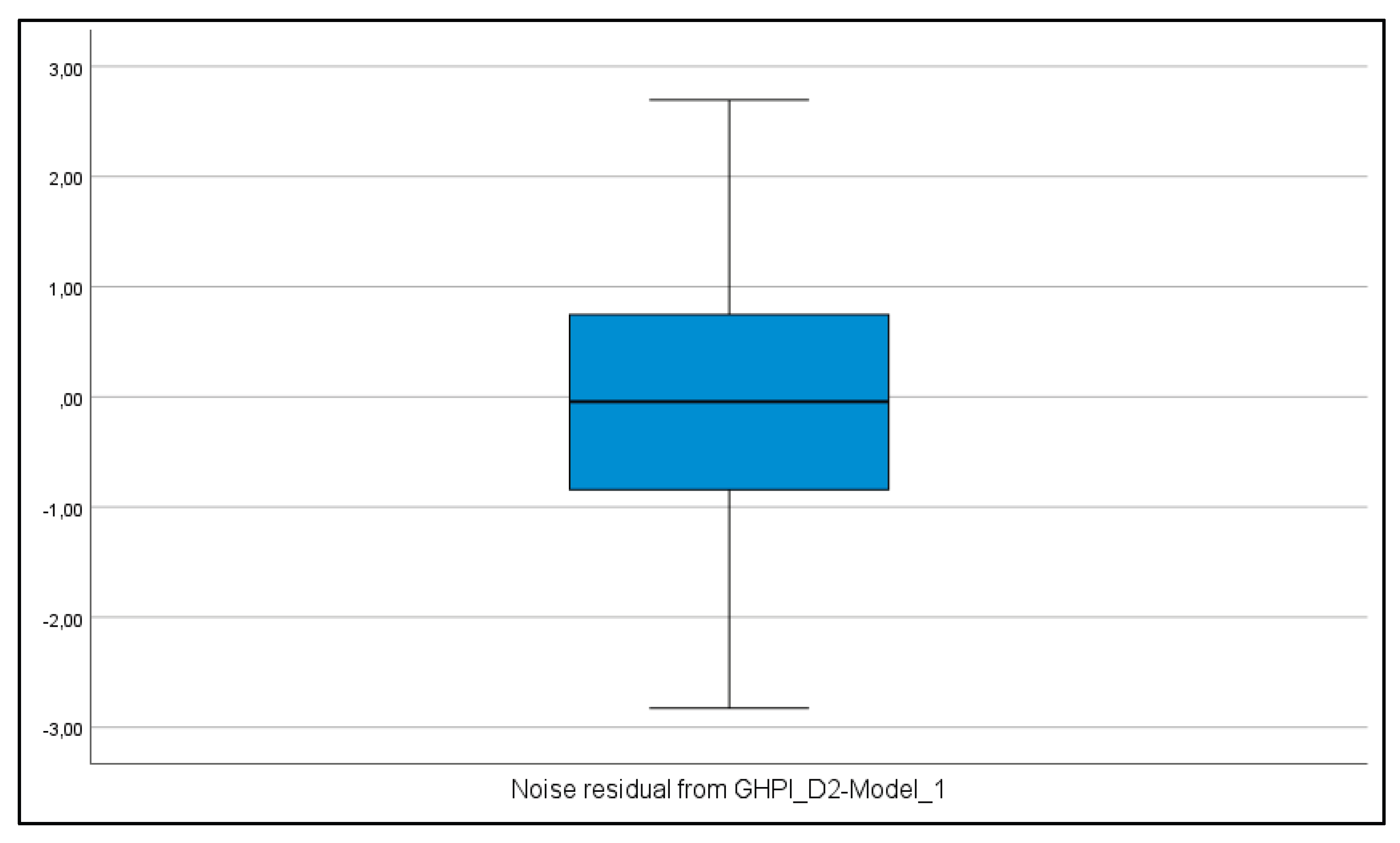
To check the normality of the residuals, Shapiro-Wilk and Kolmogorov-Smirnov tests were performed. Both tests did not show a statistically significant deviation from the normal distribution. The Shapiro-Wilk test, which is more suitable for samples with n < 50, showed W = 0.983 (p = 0.805), which is significantly above the critical value of 0.05. A high W value (close to 1) indicates a high correspondence to the normal distribution. The Kolmogorov-Smirnov test also confirms the results (K-S = 0.090, p ≥ 0.200). The graphical distribution of the test results also confirms the validity of the above conclusions (See Appendix B.3), incl. by the bell-shaped distribution of the residuals.

Table 5.
Shapiro-Wilk and Kolmogorov-Smirnov test results.
| Case Processing Summary | |||||||||||||||||||||||
| Cases | |||||||||||||||||||||||
| Valid | Missing | Total | |||||||||||||||||||||
| N | Percent | N | Percent | N | Percent | ||||||||||||||||||
| Noise residual from GHPI_D2-Model_1 | 38 | 95,0% | 2 | 5,0% | 40 | 100,0% | |||||||||||||||||
| Descriptives | |||||||||||||||||||||||
| Statistic | Std. Error | ||||||||||||||||||||||
| Noise residual from GHPI_D2-Model_1 | Mean | 0,0018 | 0,19471 | ||||||||||||||||||||
| 95% Confidence Interval for Mean | Lower Bound | -,3927 | |||||||||||||||||||||
| Upper Bound | 0,3963 | ||||||||||||||||||||||
| 5% Trimmed Mean | -0,0057 | ||||||||||||||||||||||
| Median | -0,0441 | ||||||||||||||||||||||
| Variance | 1,441 | ||||||||||||||||||||||
| Std. Deviation | 1,20025 | ||||||||||||||||||||||
| Minimum | -2,82 | ||||||||||||||||||||||
| Maximum | 2,70 | ||||||||||||||||||||||
| Range | 5,52 | ||||||||||||||||||||||
| Interquartile Range | 1,64 | ||||||||||||||||||||||
| Skewness | 0,027 | 0,383 | |||||||||||||||||||||
| Kurtosis | 0,367 | 0,750 | |||||||||||||||||||||
| Tests of Normality | |||||||||||||||||||||||
| Kolmogorov-Smirnova | Shapiro-Wilk | ||||||||||||||||||||||
| Statistic | df | Sig. | Statistic | df | Sig. | ||||||||||||||||||
| Noise residual from GHPI_D2-Model_1 | 0,090 | 38 | 0,200* | 0,983 | 38 | 0,805 | |||||||||||||||||
| *. This is a lower bound of the true significance. | |||||||||||||||||||||||
| a. Lilliefors Significance Correction | |||||||||||||||||||||||
| Coefficientsa,b | |||||||||||||||||||||||
| Model | Unstandardized Coefficients | Standar-dized Coefficients | t | Sig. | 95,0% Confidence Interval for B | Correlations | Collinearity Statistics | ||||||||||||||||
| B | Std. Error | Beta | Lower Bound | Upper Bound | Zero-order | Partial | Part | Tolerance | VIF | ||||||||||||||
| 1 | OOHE_D2 | 0,570 | 0,061 | 0,721 | 9,270 | 0,000 | 0,445 | 0,695 | 0,778 | 0,843 | 0,656 | 0,828 | 1,207 | ||||||||||
| WSMSRD_D2 | 0,215 | 0,056 | 0,331 | 3,827 | 0,001 | 0,101 | 0,329 | 0,627 | 0,543 | 0,271 | 0,670 | 1,493 | |||||||||||
| ARH_D2 | 0,347 | 0,134 | 0,218 | 2,591 | 0,014 | 0,075 | 0,619 | 0,260 | 0,401 | 0,183 | 0,706 | 1,416 | |||||||||||
| a. Dependent Variable: GHPI_D2 | |||||||||||||||||||||||
| b. Linear Regression through the Origin | |||||||||||||||||||||||
4.4.3. ARCH Effect Test
To test for conditional heteroscedasticity (ARCH effects), an ARCH LM test with 12 lags (See Table 6) was conducted, using linear regression of the squared residuals against their lags (LM test).
The regression of the squares of the residuals against their lagged values showed no statistically significant autocorrelation (F(12, 13) = 0.514, p = 0.871), further confirming that the variance of the residuals is stable over time.
5. Discussion
The ARIMAX (0,2,1) model revealed major factors in explaining house price growth in Bulgaria in the decade preceding and immediately following the announcement of Eurozone accession. From an initial set of 48 potential predictors, covering macroeconomic indicators, financial conditions, demographic trends and market factors, the data selection and stationarization procedure identified only three statistically significant predictors. This substantial reduction of the data from 48 to 3 factors suggests that house price dynamics in Bulgaria are driven by a focused set of fundamental drivers, rather than a multidimensional set of influences.
This finding has important potential implications for both theory and policy. First, the simplified three-factor regression model challenges the notion that housing markets in transition countries require complex multidimensional frameworks for adequate explanation. Instead, our results show that even during a period of profound institutional change – including maintaining a currency board, consolidating EU membership and eventually joining the Eurozone – house price growth responds systematically to a limited number of key variables. This simplicity is consistent with recent evidence from other Central and Eastern European markets, where fundamental factors dominate over speculative effects or institutional context.
Second, the statistical significance of the final ARIMAX model over the entire sample period 2015-2025 is particularly striking. The data set covers three distinct phases: pre-convergence (2015-2019), pandemic disruptions (2020-2021) and finally preparation and entry into the Eurozone (2022-2025). The fact that the same three factors remain statistically significant across these regime changes suggests structural stability in the determinants of Bulgarian house prices. This stability may reflect the effect of the currency board mechanism, which pegged the lev to the German mark in 1997 and then automatically to the euro. In this way, Bulgaria adapts its business cycle curve ex ante to the Eurozone countries through the effect of nominal convergence, especially in its currency context, well before formal membership with a clear national specificity, different from the experience with Croatia (Visković & Čipčić, 2025) and its admission to the Eurozone on 1.1.2023.
Third, the transition to euro adoption in January 2026 provides a natural quasi-experiment to assess whether the identified factors retain their explanatory power under a new currency regime (Marinov, 2017). The last quarters of our sample (Q4 2024 – Q3 2025) capture the period immediately before accession, during which expectations of euro adoption strongly influenced both housing demand and credit conditions. Preliminary data from 2025 do not suggest a structural break in the relationship between the three key factors and house price growth, suggesting that the currency change itself may have had a limited independent impact – possibly because markets have already priced in price convergence under the currency board arrangement. However, several caveats are worth noting. First, although a developed down-up procedure is effective in identifying significant predictors, it requires substantiation of economic arguments for the established causal relationship, which transcend the purely mathematical logic of the conclusions. The observed associations between the three predictors and house prices do not exclude the influence of other factors for which there is no data for the entire period studied or the data are partial, or their access is highly restricted or it is impossible to obtain them publicly. Second, the quarterly frequency of observations – although standard in macroeconomic housing research – may conceal dynamics with a higher frequency, especially during periods of rapid institutional change (Mihaylova-Borisova & Nenkova, 2020). Third, the performance of the model during the period of accession to the Eurozone should be carefully monitored, since structural changes in the available bank resources for lending, cross-border capital flows or mortgage market integration could change the factor weights or introduce new predictors. The latter is particularly interesting in view of the release by the Central Bank of Bulgaria to commercial banks of a large-scale credit resource through the mechanism of the minimum reserve requirement ratio. Specific to the ECB and the BNB is the gap of over 10% in favor of Bulgaria, which releases a large-scale new credit resource to support the market forces of housing demand in Bulgaria, ceteris paribus.
Looking ahead, the three-factor ARIMAX model offers a practical tool for policymakers and central bankers monitoring housing market stability in the post-accession phase of Bulgaria. If the three-component structure of the descriptors is maintained, it will provide a focused set of indicators for monitoring and designing macroprudential policy. Furthermore, Bulgaria’s experience as the 21st and newest member of the Eurozone offers valuable insights for subsequent candidate countries. Among them, we include those with low exchange rate volatility between their national currencies and the euro, which again puts the focus on the important condition for the existence of objective consequences and impacts of currency integration on the housing market (Visković & Čipčić, 2025).
Future research should extend the analysis beyond 2025 to assess the stability of the model in the event of full euro adoption in Bulgaria (with the cessation of price announcements in the old national currency as a regulatory requirement by 8.8.2026), disaggregate national trends by regional markets, and examine potential nonlinear or threshold effects that the ARIMAX model may objectively ignore.
Future research could also consider the search for sustainable solutions with the housing stock and civil construction activities (Gabriela, Nijkamp, & Kourtit, 2023) in the post-war reconstruction of Ukraine (Sukhomud & Shnaider, 2023). International experience in the physical restoration of housing and the restoration of its value after structural changes or catastrophic risks (Ishiwatari, Ranghieri, Taniguchi, & Mimura, 2021) can be fully beneficial for decision-making today (Ishiwatari, Sakamoto, & Nakayama, 2025), even before the war ends.
6. Conclusions
This study provides new evidence on the factors that determine the dynamics of house prices in Bulgaria in the specific context of the transition from a long-standing currency board regime to Eurozone membership. By applying an ARIMAX(0,2,1) model on 40 quarterly observations for the period 2015Q4-2025Q3, the study successfully identifies the key determinants of the acceleration in real estate prices. The results obtained reveal that the dynamics of house prices in Bulgaria is explained by three specific factors: the homeowners’ expenditure index, average rents and the utility expenditure index. The three predictors demonstrate statistical significance at the 1% level, which indicates their strong and persistent effects. The model explains the variation in house price acceleration with low mean square error and has high explanatory power. Particularly significant is the conclusion that traditional macroeconomic, demographic, financial and sectoral factors do not show a statistically significant relationship with price dynamics for the studied ten-year period. This result provokes a reconsideration of conventional theoretical approaches to housing pricing in the context of economies in transition. While the classical literature emphasizes the role of interest rates, economic growth, income and demographic changes, the present study demonstrates that in the specific conditions of Bulgaria these factors give way to country-specific determinants. The established relationship between housing prices and the costs of ownership, rents and utilities reveals an important pricing mechanism, in which current operating costs have a stronger influence than traditional macroeconomic variables. This can be explained by the specifics of the Bulgarian real estate market, where the long-standing currency board has ensured a stable convergent environment, and the process of approval of Bulgaria’s membership in the Eurozone is reflected in the expectations for price convergence with European levels ahead of schedule. The diagnostic analysis confirms the statistical significance of the model with the absence of autocorrelation in the residuals and successful capture of all systematic information in the data. The non-parametric correlation analysis further validates the statistically significant monotonic relationships between the regressors and the dependent variable, which strengthens the confidence in the obtained results. From a methodological point of view, the use of second differentiation in the ARIMAX model proves to be an adequate approach for modeling the acceleration in prices, successfully overcoming the problems with non-stationarity in historical data, which are influenced by three specific sub-periods: pre-convergence (2015-2019), pandemic disruptions (2020-2021) and finally - preparation and entry into the Eurozone (2022-2025). The results of the study have important practical applications for the development of policies in the housing sector. The focus on specific national factors shows that measures to regulate the real estate market should take into account local specificities, and not blindly follow general macroeconomic recipes. Regulators should pay special attention to policies related to property and utility costs, as they have a direct impact on price dynamics. In conclusion, this study contributes to a better understanding of housing pricing mechanisms in the specific context of a small open economy undergoing currency convergence. It demonstrates the need to develop models that take into account national specificities, rather than mechanically applying theories developed for developed markets with different institutional characteristics.
Author Contributions
Conceptualization, A.Z., G.Z. and LS; methodology, A.Z, G.Z., L.S. and M.O.; software, G.Z.; validation, A.Z., G.Z., L.S. and M.O.; formal analysis, A.Z. and G.Z.; investigation, A.Z., G.Z., L.S. and M.O.; resources, A.Z., G.Z., L.S. and M.O.; data curation, A.Z. and G.Z.; writing—original draft preparation, A.Z. and G.Z.; writing—review and editing, A.Z., G.Z. and L.S.; visualization, A.Z., G.Z. and M.O.; supervision, A.Z., G.Z. and L.S.; project administration, A.Z. and G.Z.; funding acquisition, A.Z All authors have read and agreed to the published version of the manuscript.
Funding
This research received no external funding.
Institutional Review Board Statement
Not applicable.
Informed Consent Statement
Not applicable.
Data Availability Statement
The data used in this paper mainly come from Eurostat, NSI, BNB and BSE.
Conflicts of Interest
The authors declare no conflicts of interest.
Appendix A
Appendix A.1. Independent and Dependent Variables
The initial stage of the study in search of a model for analysis and assessment of the dynamics of the GHPI of Bulgaria (with constituent analytical indices HPINH, HPIEH) for the period 2015Q4–2025Q3 is the selection of influencing factors and their grouping. Based on 4 main sources – BNB, NSI, Eurostat and BSE, an econometric assessment was carried out, 48 factors were selected, including aggregated and disaggregated, distributed into seven main groups.
Table A1.
Selection and grouping of independent and dependent variables.
| № | Group | Number of factors | № | Selected variables – first stage | Factor code | Source: |
| Y. | Independent variables |
3 | 1 | General house price index (2015=100) | GHPI | NSI |
| 2 | HPI New homes (2015=100) | HPINH | NSI | |||
| 3 | HPI Existing homes (2015=100) | HPIEH | NSI | |||
| A. | Macro factor | 5 | 1 | Gross Domestic Product ('000 EUR) | GDP | NSI |
| 2 | Export ('000 EUR) | EXP | NSI | |||
| 3 | Import ('000 EIR) | IMP | NSI | |||
| 4 | HICP (2015=100) | HICP | NSI | |||
| 5 | GDP per capita | GDPpC | Eurostat | |||
| B. | Housing Services / HS | 7 | 6 | Owner-occupiers housing expenditures (Index 2015=100) | OOHE | NSI |
| 7 | Acquisitions of dwellings (Index 2015=100) | AD | NSI | |||
| 8 | Other services related to the acquisitions of dwellings (Index 2015Q4=100) | OSRAD | NSI | |||
| 9 | Ownership of dwellings (Index 2015Q4=100) | OD | NSI | |||
| 10 | Major repairs and maintenance (Index 2015Q4=100) | MRM | NSI | |||
| 11 | Other services related to ownership of dwellings (Index 2015Q4=100) | OSROD | NSI | |||
| 12 | Insurance connected with the dwelling (Index 2015Q4=100) | ICD | NSI | |||
| C. | Energy and Comunal Services / ECS | 16 | 13 | Housing, water, electricity, gas and other fuels (Index 2015Q4=100) | HWEGOF | NSI |
| 14 | Actual rentals for housing (Index 2015Q4=100) | ARH | NSI | |||
| 15 | Maintenance and repair of the dwelling (Index 2015Q4=100) | MRD | NSI | |||
| 16 | Materials for the maintenance and repair of the dwelling (Index 2015Q4=100) | MMRD | NSI | |||
| 17 | Services for the maintenance and repair of the dwelling (Index 2015Q4=100) | SMRD | NSI | |||
| 18 | Water supply and miscellaneous services relating to the dwelling (Index 2015Q4=100) | WSMSRD | NSI | |||
| 19 | Water supply (Index 2015Q4=100) | WS | NSI | |||
| 20 | Refuse collection (Index 2015Q4=100) | RC | NSI | |||
| 21 | Sewage collection (Index 2015Q4=100) | SC | NSI | |||
| 22 | Other services relating to the dwelling n.e.c. (Index 2015Q4=100) | OSRD | NSI | |||
| 23 | Electricity, gas and other fuels (Index 2015Q4=100) | EGOF | NSI | |||
| 24 | Electricity (Index 2015Q4=100) | E | NSI | |||
| 25 | Gas (Index 2015Q4=100) | G | NSI | |||
| 26 | Solid fuels (Index 2015Q4=100) | SF | NSI | |||
| 27 | Heat energy (Index 2015Q4=100) | HE | NSI | |||
| 28 | Furnishings, household equipment and routine household maintenance (Index 2015Q4=100) | FHERHM | NSI | |||
| D | Construction | 8 | 29 | Newly built residential buildings completed | NBRBC | NSI |
| 30 | Newly built dwelling completed by rooms - total | NBDCRT | NSI | |||
| 31 | Newly built dwelling completed by rooms - 1 room | NBDC1R | NSI | |||
| 32 | Newly built dwelling completed by rooms - 2 rooms | NBDC2Rs | NSI | |||
| 33 | Newly built dwelling completed by rooms - 3 rooms | NBDC3Rs | NSI | |||
| 34 | Newly built dwelling completed by rooms - 4 rooms | NBDC4Rs | NSI | |||
| 35 | Newly built dwelling completed by rooms - 5 rooms | NBDC5Rs | NSI | |||
| 36 | Newly built dwelling completed by rooms - 6+ rooms | NBDC6Rs | NSI | |||
| E | Income & Labor market / ILM | 3 | 37 | Average gross monthly wages and salaries (Index 2015Q4=100) | AGQWS | NSI |
| 38 | Unemployment coefficient (Index 2015Q4=100) | UNEMPL | NSI | |||
| 39 | Labor Force in '000 | LF | NSI | |||
| F | Credits / Cr | 6 | 40 | Dwelling credits | DwCr | BNB |
| 41 | Interest Rate | IRATE | BNB | |||
| 42 | Bank loans secured by residential property (Index 2015Q4=100) | BLSRP | BNB | |||
| 43 | Household interest costs on mortgage loans | HICML | BNB | |||
| 44 | Bad and restructured housing loans | BRHL | BNB | |||
| 45 | Interest Rate for Mortgage in BGN | IRATEMp | BNB | |||
| G | Investment & Wealth / InvW | 3 | 46 | Net foreign investment in real estate | NFIP | BNB |
| 47 | EUR/USD | ExR | BNB | |||
| 48 | BSE index SOFIX | Sofix | BSE | |||
| Number of factors 1st stage: | 48 | Number of groups 1st stage: | 7 | |||
Legend: NSI – National Statistical Institute of Bulgaria; BNB – Bulgarian National Bank, BSE – Bulgarian Stock Exchange; Eurostat – Statistical office of the European Union.
Appendix A.2. Descriptive Statistics
Selected indicators with results from descriptive statistics for the historical data of the 48 descriptors and the three independent variables HPI, HPINH, HPIEH in Bulgaria for the period 2015Q4-2025Q3 are presented in the following table.
Table A2.
Descriptive statistics of historical data of dependent variables and independent variables from groups A-G.
Table A2.
Descriptive statistics of historical data of dependent variables and independent variables from groups A-G.
| Factor code | Source: | Data type | Change t40/t1 | AVE | STDEV | CV |
| GHPI | NSI | Index | 2.5601 | 154.95 | 43.05 | 27.78% |
| HPINH | NSI | Index | 2.3224 | 147.52 | 37.00 | 25.08% |
| HPIEH | NSI | Index | 2.7154 | 159.51 | 47.00 | 29.47% |
| GDP | NSI | EUR | 2.7504 | 18308.11 | 5683.54 | 31.04% |
| EXP | NSI | EUR | 2.7063 | 10371.31 | 3758.78 | 36.24% |
| IMP | NSI | EUR | 2.1661 | 10398.46 | 3248.34 | 31.24% |
| HICP | NSI | Index | 1.4338 | 115.49 | 16.05 | 13.90% |
| GDPpC | Eurostat | Euro | 2.7268 | 2793.50 | 934.67 | 33.46% |
| OOHE | NSI | Index | 2.1634 | 139.65 | 33.27 | 23.82% |
| AD | NSI | Index | 2.2843 | 144.32 | 36.65 | 25.40% |
| OSRAD | NSI | Index | 2.5820 | 153.47 | 46.22 | 30.12% |
| OD | NSI | Index | 1.4776 | 115.09 | 14.36 | 12.48% |
| MRM | NSI | Index | 1.7211 | 122.57 | 24.58 | 20.06% |
| OSROD | NSI | Index | 1.2874 | 108.90 | 7.30 | 6.71% |
| ICD | NSI | Index | 0.9893 | 99.67 | 2.33 | 2.33% |
| HWEGOF | NSI | Index | 1.6315 | 122.66 | 21.57 | 17.59% |
| ARH | NSI | Index | 1.5209 | 115.32 | 14.80 | 12.84% |
| MRD | NSI | Index | 1.6091 | 121.24 | 22.51 | 18.57% |
| MMRD | NSI | Index | 1.5256 | 119.51 | 20.60 | 17.24% |
| SMRD | NSI | Index | 1.8381 | 125.11 | 27.45 | 21.94% |
| WSMSRD | NSI | Index | 1.9384 | 129.22 | 27.97 | 21.65% |
| WS | NSI | Index | 1.9879 | 132.87 | 32.62 | 24.55% |
| RC | NSI | Index | 1.5435 | 111.97 | 14.96 | 13.36% |
| SC | NSI | Index | 2.9131 | 162.41 | 56.05 | 34.51% |
| OSRD | NSI | Index | 2.0591 | 134.42 | 30.54 | 22.72% |
| EGOF | NSI | Index | 1.5847 | 123.50 | 21.77 | 17.62% |
| E | NSI | Index | 1.4123 | 112.80 | 11.48 | 10.18% |
| G | NSI | Index | 1.5689 | 137.84 | 66.51 | 48.26% |
| SF | NSI | Index | 1.9437 | 146.31 | 44.41 | 30.35% |
| HE | NSI | Index | 1.8766 | 137.31 | 32.95 | 23.99% |
| FHERHM | NSI | Index | 1.2670 | 108.90 | 11.49 | 10.55% |
| NBRBC | NSI | Number | 2.2025 | 935.45 | 345.63 | 36.95% |
| NBDCRT | NSI | Number | 3.2455 | 3832.63 | 1513.38 | 39.49% |
| NBDC1R | NSI | Number | 2.1889 | 306.25 | 129.48 | 42.28% |
| NBDC2Rs | NSI | Number | 3.4496 | 1457.73 | 578.79 | 39.71% |
| NBDC3Rs | NSI | Number | 3.5357 | 1295.30 | 531.94 | 41.07% |
| NBDC4Rs | NSI | Number | 3.1563 | 430.03 | 194.75 | 45.29% |
| NBDC5Rs | NSI | Number | 2.6422 | 184.68 | 89.87 | 48.66% |
| NBDC6Rs | NSI | Number | 2.5773 | 158.65 | 93.80 | 59.13% |
| AGQWS | NSI | Number | 2.8253 | 171.64 | 56.09 | 32.68% |
| UNEMPL | NSI | Index | 0.4304 | 64.30 | 16.51 | 25.67% |
| LF | NSI | Number | 0.9211 | 3195.37 | 142.97 | 4.47% |
| DwCr | BNB | Mln. Euro | 2.8939 | 14572.86 | 5049.09 | 34.65% |
| IRATE | BNB | Index | 0.4192 | 57.17 | 16.86 | 29.49% |
| BLSRP | BNB | Index | 3.8291 | 179.02 | 78.45 | 43.82% |
| HICML | BNB | Euro | 1.5923 | 68.30 | 16.61 | 24.32% |
| BRHL | BNB | Mln. Euro | 0.1330 | 1040.44 | 596.75 | 57.36% |
| IRATEMp | BNB | Percent | 0.4218 | 3.73 | 1.10 | 29.46% |
| NFIP | BNB | Index | 1.1186 | 107.03 | 5.14 | 4.80% |
| ExR | BNB | USD | 1.0746 | 1.12 | 0.05 | 4.84% |
| Sofix | BSE | Number | 2.3315 | 640.90 | 157.68 | 24.60% |
Source: Calculations of the authors.
Appendix A.3. Historical Dynamics of First-Order Differential Data
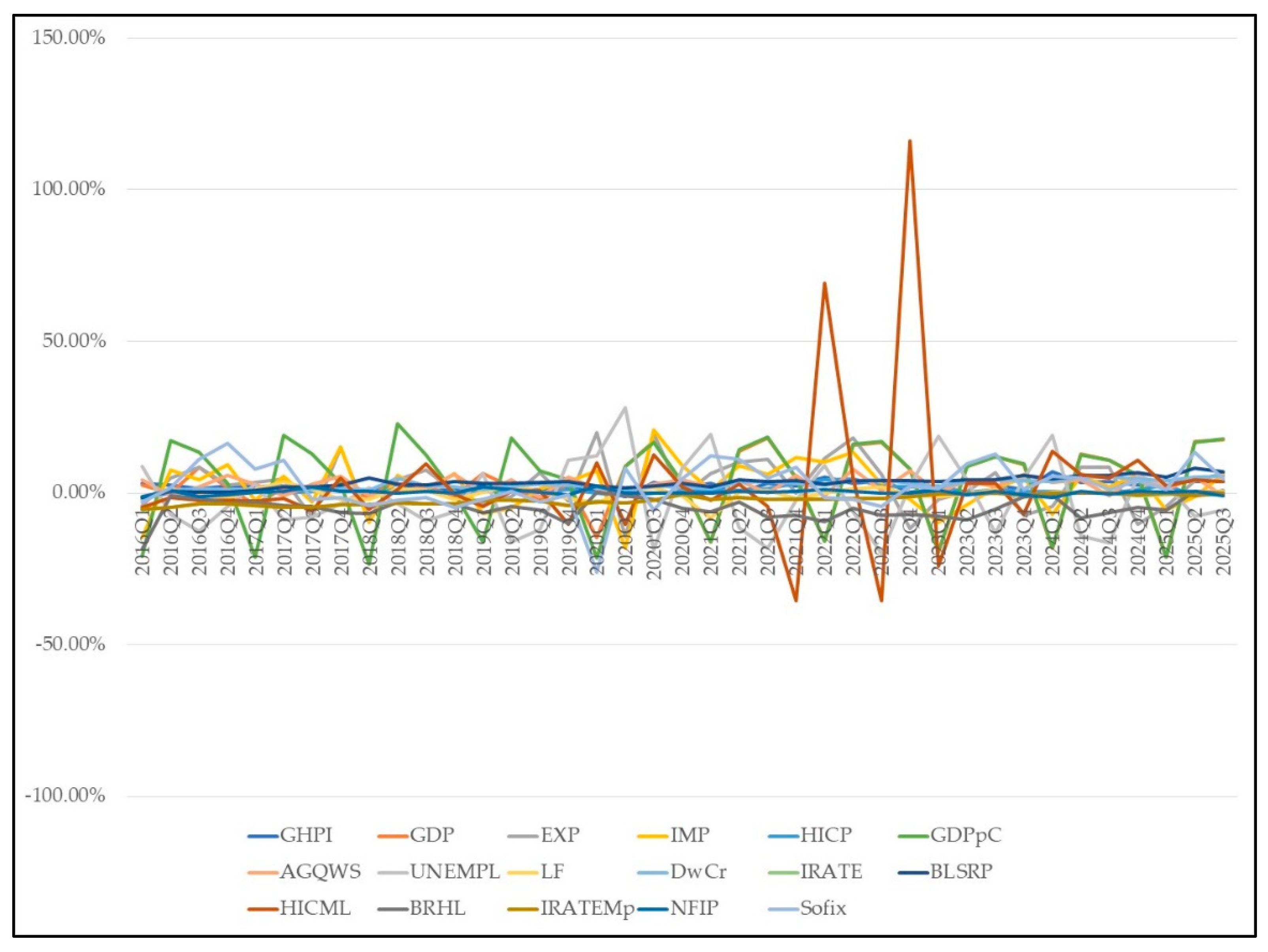
After establishing non-stationarity of the historical data, a first-differential data estimate is made for both the dependent and independent variables. Figure A3 presents the relative changes in the values of the indicators for the period 2015Q4-2025Q3 calculated on a chain-wise basis with a number of observations N=39: (t2-t1)/t1.
Figure A3.
Dynamics of the first differential of the variables of groups A, F, G & E.
Appendix B
Appendix B.1. First Differencing of Variables with a Statistically Significant Impact on GHPI, Selected in the ARIMAX (0,2,1) Model
Figure B1.
Dynamics of the first differentiated factors in the ARIMAX model (0,2,1): OOHE, AHE & WSMSRD with a statistically significant impact on GHPI.
Figure B1.
Dynamics of the first differentiated factors in the ARIMAX model (0,2,1): OOHE, AHE & WSMSRD with a statistically significant impact on GHPI.
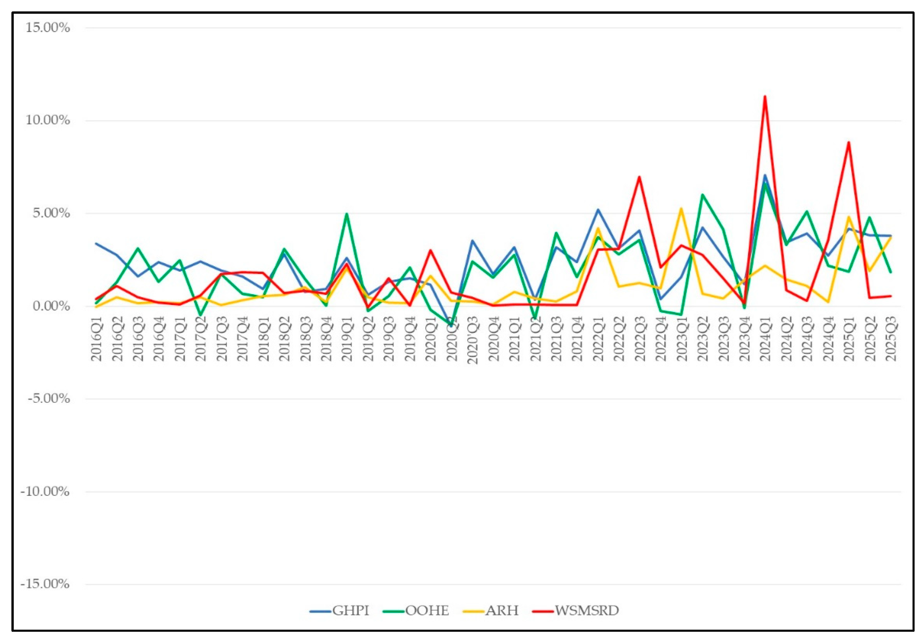
Figure A3.
Dynamics of the first differential of the variables of groups A, F, G & E.

Appendix B.2. Descriptive Statistics of Second Deference of the Dependent Variable GHPI_D2 and Independent Variables
Table B2.
Descriptive Statistics of GHPI_D2, OOHE_D2, WSMSRD_D2 and ARH_D2.
| GHPI_D2 | OOHE_D2 | WSMSRD_D2 | ARH_D2 | ||
| N | Valid | 38 | 38 | 38 | 38 |
| Missing | 2 | 2 | 2 | 2 | |
| Mean | 0,157 | 0,099 | 0,017 | 0,143 | |
| Std. Error of Mean | 0,546 | 0,691 | 0,841 | 0,342 | |
| Median | -0,39 | -0,39 | 0,00 | -0,02 | |
| Mode | -6,53a | -6,89a | -15,61a | -5,52a | |
| Std. Deviation | 3,36 | 4,26 | 5,18 | 2,11 | |
| Variance | 11,31 | 18,12 | 26,88 | 4,45 | |
| Skewness | 0,853 | 0,592 | -0,258 | 0,407 | |
| Std. Error of Skewness | 0,383 | 0,383 | 0,383 | 0,383 | |
| Kurtosis | 2,35 | 0,35 | 5,51 | 2,89 | |
| Std. Error of Kurtosis | 0,750 | 0,750 | 0,750 | 0,750 | |
| Range | 17,87 | 18,14 | 32,48 | 11,83 | |
| Minimum | -6,53 | -6,89 | -15,61 | -5,52 | |
| Maximum | 11,34 | 11,25 | 16,87 | 6,31 | |
| Sum | 5,98 | 3,75 | 0,63 | 5,43 | |
| a. Multiple modes exist. The smallest value is shown | |||||
Appendix B.3. Graphical Evidence from the Test for Normal Distribution of Residuals
Figure B3-1.
Histogram results.
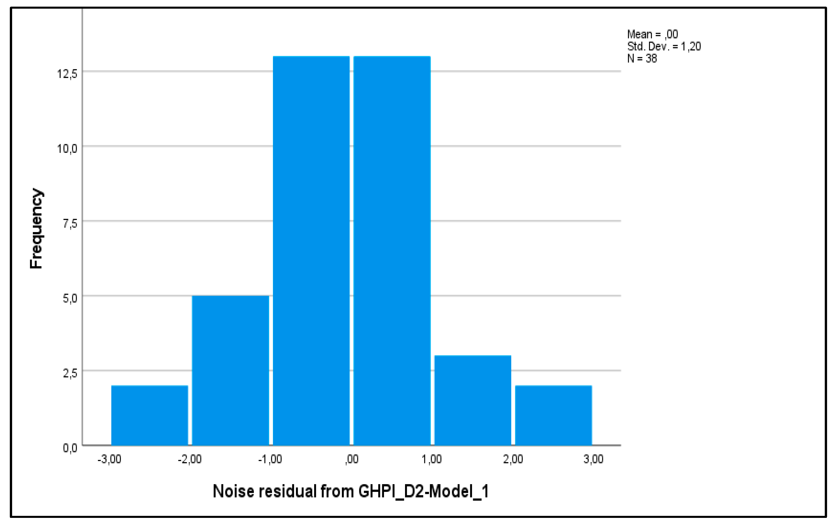
Figure B3-2.
Normal Q-Q Plot of Noise residual from GHPI_D2-Model_1.
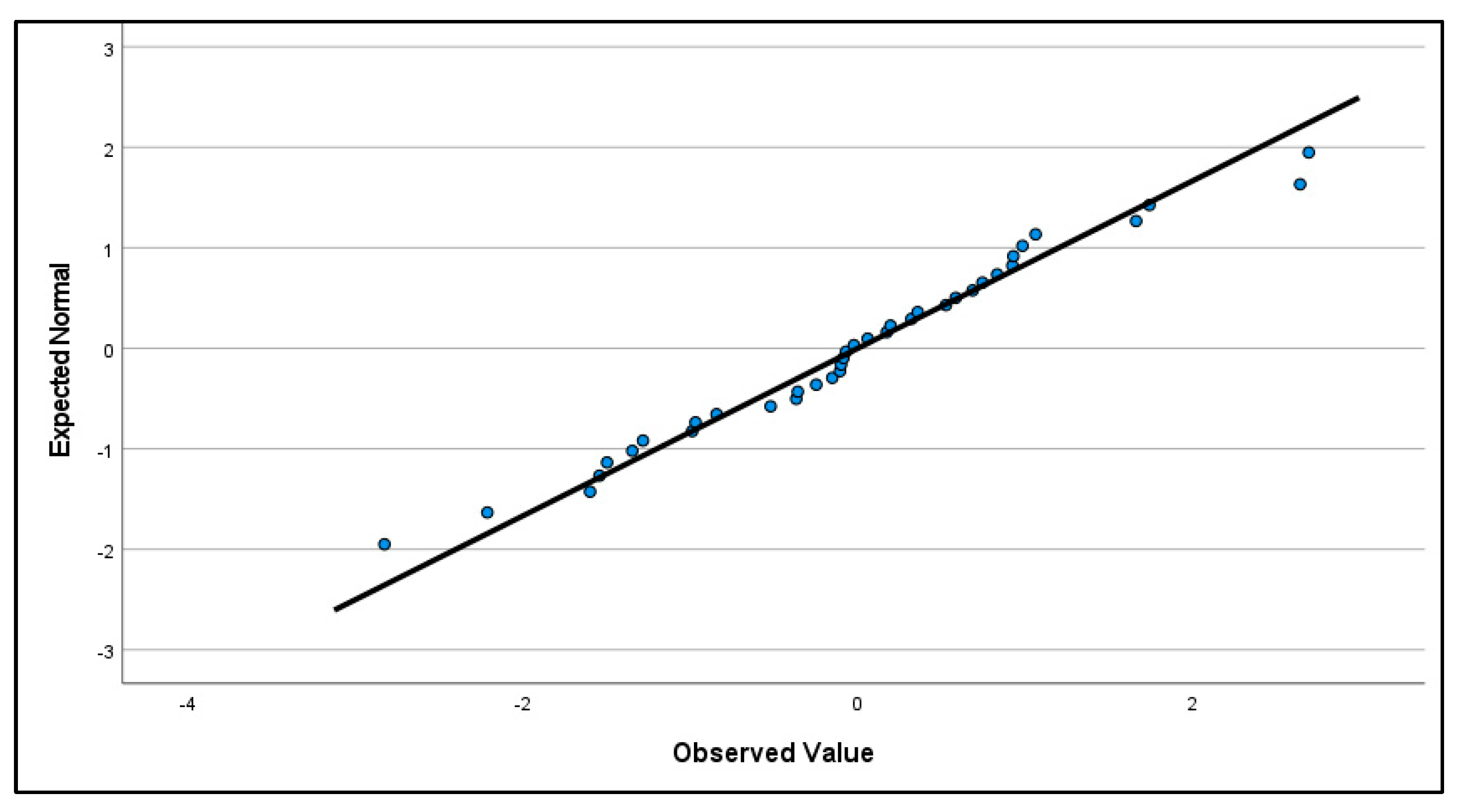
Figure B3-3.
Detrended Normal Q-Q Plot of Noise residual from GHPI_D2-Model_1.
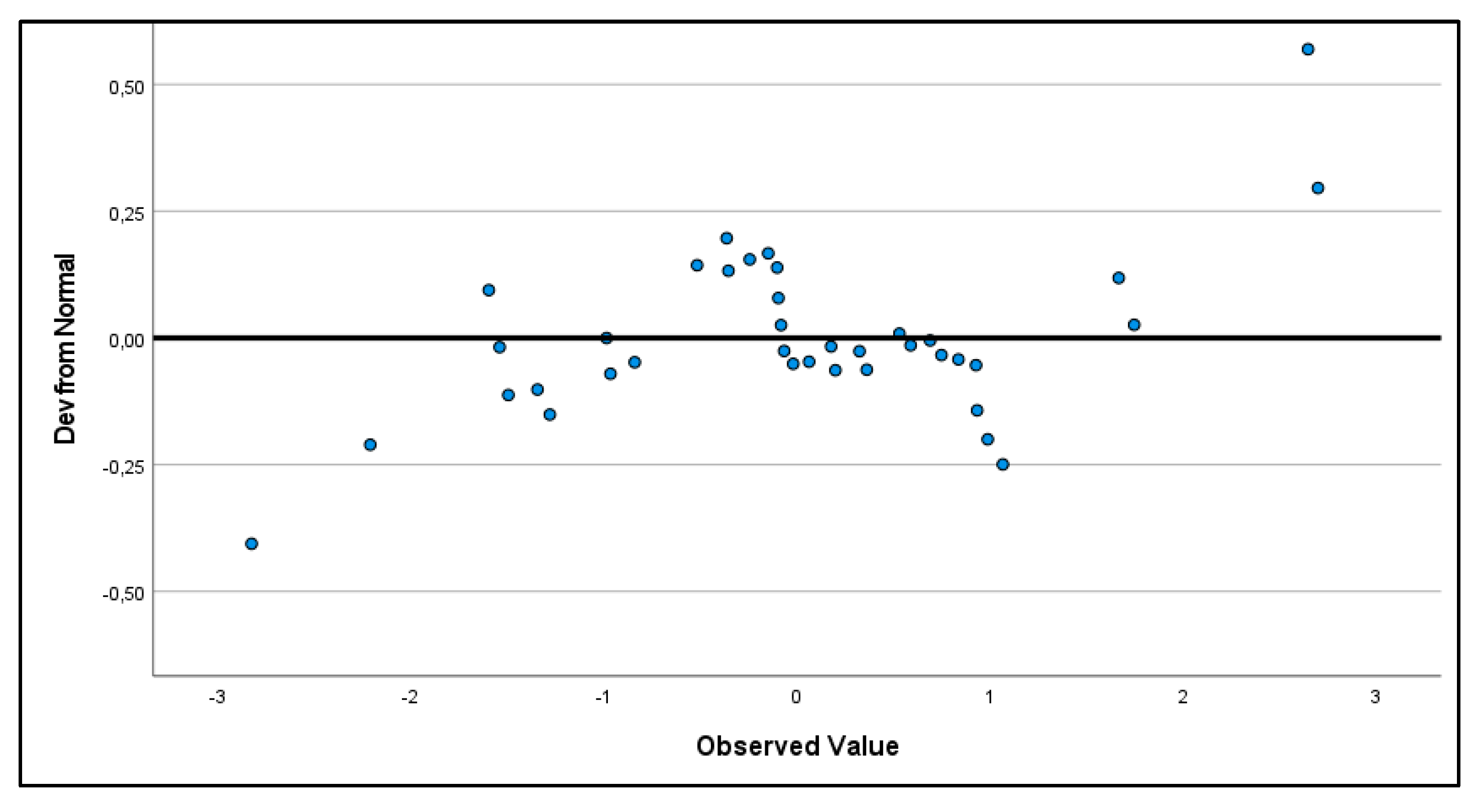
Figure B3-4.
Distribution of Noise residual from GHPI_D2-Model_1.
References
- Algieri, B. House Price Determinants: Fundamentals and Underlying Factors. Comparative Economic Studies 2013, 55, 315–341. [Google Scholar] [CrossRef]
- Anari, A.; Kolari, J. House Prices and Inflation. Real Estate Economics 2002, 30, 67–84. [Google Scholar] [CrossRef]
- Araya, F.; Poblete, P.; Salazar, L. A.; Sánchez, O.; Sierra-Varela, L.; Filun, Á. Exploring the Influence of Construction Companies Characteristics on Their Response to the COVID-19 Pandemic in the Chilean Context. Sustainability 2024, 16, 3417. [Google Scholar] [CrossRef]
- Atanassov, A.; Trifonova, S.; Saraivanova, J.; Pramatarov, A. Assessment of the Administrative Burdens for Businesses in Bulgaria According to the National Legislation Related to the European Union Internal Market. Management: Journal of Contemporary Management Issues 2017, 22(Special Issue), 21–49. Available online: http://moj.efst.hr/management/Vol22-Specissue/2_Atanassov_et_al.pdf.
- Aydinli, S. Impact of unexpected conditions on construction cost forecasting performance: evidence from Europe. Construction Management and Economics 2024, 42, 787–801. [Google Scholar] [CrossRef]
- Caldera Sánchez, A.; Johansson, Å. The Price Responsiveness of Housing Supply in OECD Countries. OECD Economics Department Working Papers 2011, 837, 1–35. [Google Scholar] [CrossRef]
- Cermáková, K.; Hromada, E. Change in the Affordability of Owner-Occupied Housing in the Context of Rising Energy Prices. Energies 2022, 15, 1281. [Google Scholar] [CrossRef]
- Ciarlone, A. House price cycles in emerging economies. Studies in Economics and Finance 2015, 32, 17–52. [Google Scholar] [CrossRef]
- Ciot, M.-G. Implementation Perspectives for the European Green Deal in Central and Eastern Europe. Sustainability 2022, 14, 3947. [Google Scholar] [CrossRef]
- Cohen, V.; Karpavičiūtė, L. The analysis of the determinants of housing prices. Independent Journal of Management & Production 2017, 8, 49–63. [Google Scholar] [CrossRef]
- Dandashly, A.; Verdun, A. Euro adoption policies in the second decade - the remarkable cases of the Baltic States. Economic and Monetary Union at Twenty 2021, 83–109. Available online: https://bit.ly/4cxxl17.
- Dickey, D. A.; Fuller, W. A. Likelihood Ratio Statistics for Autoregressive Time Series with a Unit Root. Econometrica 1981, 49, 1057–1072. [Google Scholar] [CrossRef]
- Distaso, W. Testing for unit root processes in random coefficient autoregressive models. Journal of Econometrics 2008, 142, 581–609. [Google Scholar] [CrossRef]
- Doling, J.; Ronald, R. Home ownership and asset-based welfare. Journal of Housing and the Built Environment 2010, 25, 165–173. [Google Scholar] [CrossRef]
- Ebekozien, A. A.; Aigbedion, M. Construction industry post-COVID-19 recovery: Stakeholders perspective on achieving sustainable development goals. International Journal of Construction Management 2021, 23, 1376–1386. [Google Scholar] [CrossRef]
- Egert, B.; Mihaljek, D. Determinants of House Prices in Central and Eastern Europe. Comparative Economic Studies 2007, 49, 337–489. [Google Scholar] [CrossRef]
- European Commission. Convergence Report 2025 on Bulgaria . D.-G. f. Affairs 2025. [Google Scholar] [CrossRef]
- European Parliament. Topics European Parliament . Retrieved 1 2, 2026, from The housing crisis in Europe: key facts and EU action (infographics). 2025. Available online: https://www.europarl.europa.eu/topics/en/article/20241014STO24542/.
- Eurostat. Housing in Europe – 2025 edition. In Housing in Europe – 2025 edition (Interactive publication); Luxemburg, Luxemburg, 2025a. [Google Scholar] [CrossRef]
- Eurostat. Gross domestic product at market prices. In National accounts indicator (ESA 2010): Gross domestic product at market prices; Luxemburg, Luxemburg, 2025b. [Google Scholar] [CrossRef]
- Eurostat. House price and sales index. House price index (2015 = 100) - annual data. Luxembourg, Luxembourg, Luxembourg. 2026a. Available online: https://ec.europa.eu/eurostat/databrowser/view/prc_hpi_a/default/table?lang=en.
- Eurostat. Distribution of population by tenure status, type of household and income group; Luxemburg, Luxemburg, 2026b. [Google Scholar] [CrossRef]
- Eurostat. Unemployment statistics. Изтегленo на 31 1 2026 r. oт Statistics Explained. 2026c. Available online: https://bit.ly/4avgdXe.
- Gabriela, C. P.; Nijkamp, P.; Kourtit, K. Regional science knowledge needs for the recovery of the Ukrainian spatial economy: A Q-analysis. Regional Science Policy & Practice 2023, 15, 75–95. [Google Scholar] [CrossRef]
- Girouard, N.; Kennedy, M.; Noord, P. v.; André, C. Recent House Price Developments: The Role of Fundamentals. OECD Economics Department Working Papers 2006, 475, 1–61. [Google Scholar] [CrossRef]
- Gönül, İ. Ö.; Omay, T. Dynamic market efficiency assessment in sustainability indices: Rolling fractional integration analysis with multiple estimators. Borsa Istanbul Review 2025, 25, 1645–1662. [Google Scholar] [CrossRef]
- Gurmu, A. T.; Krezel, A.; Ongkowijoyo, C. Fuzzy-stochastic model to assess defects in low-rise residential buildings. Journal of Building Engineering 2021, 40, 102318. [Google Scholar] [CrossRef]
- Haandrikman, K.; Costa, R.; Malmberg, B.; Rogne, A. F.; Sleutjes, B. Socio-economic segregation in European cities. A comparative study of Brussels, Copenhagen, Amsterdam, Oslo and Stockholm. Urban Geography 2023, 44, 1–36. [Google Scholar] [CrossRef]
- Herrera, R. F.; Sánchez, O.; Castañeda, K.; Porras, H. Cost Overrun Causative Factors in Road Infrastructure Projects: A Frequency and Importance Analysis. Applied Sciences 2020, 10, 5506. [Google Scholar] [CrossRef]
- Hyndman, R. J.; Koehler, A. B. Another look at measures of forecast accuracy. International Journal of Forecasting 2006, 22, 679–688. [Google Scholar] [CrossRef]
- Idirizov, B. Analysis of the Bulgarian Housing Price Index: Risks, Market Dynamics, and Economic Implications. Economic Studies (Ikonomicheski Izsledvania) 2025, 34, 175–195. Available online: https://www.econ-studies.iki.bas.bg/articles/Pr4gir8HxtKopH7BWNaC.
- Iliopoulou, P.; Krassanakis, V.; Kappelos, K. Modeling the Spatial Impact of Short-Term Rentals on House Prices: The Case of Athens, Greece. Urban Science 2025, 9, 539. [Google Scholar] [CrossRef]
- Irandoust, M. House prices and unemployment: an empirical analysis of causality. International Journal of Housing Markets and Analysis 2019, 12, 148–164. [Google Scholar] [CrossRef]
- Ishiwatari, M.; Ranghieri, F.; Taniguchi, K.; Mimura, S. Learning from Megadisasters in Japan: Sharing Lessons with the World. Journal of Disaster Research 2021, 16, 942–946. [Google Scholar] [CrossRef]
- Ishiwatari, M.; Sakamoto, A.; Nakayama, M. Expediting Recovery: Lessons and Challenges from the Great East Japan Earthquake to War-Torn Ukraine. Sustainability 2025, 17, 1210. [Google Scholar] [CrossRef]
- Kotu, V.; Deshpande, B. Chapter 12 - Time Series Forecasting,. От V. Kotu, & B. Deshpande, Data Science (Second Edition); Morgan Kaufmann, 2019; pp. стр. 395–445. [Google Scholar] [CrossRef]
- Kuang, W.; Liu, P. Inflation and House Prices: Theory and Evidence from 35 Major Cities in China. International Real Estate Review 2015, 18, 217–240. Available online: https://www.gssinst.org/irer/2020/04/28/inflation-and-house-prices-theory-and-evidence-from-35-major-cities-in-china/. [CrossRef]
- Li, B.; Zeng, Z. Fundamentals behind house prices. Economics Letters 2010, 108, 205–207. [Google Scholar] [CrossRef]
- Lin, Y.-C.; Lee, C. L.; Newell, G. Varying interest rate sensitivity of different property sectors: cross-country evidence from REITs. Journal of Property Investment & Finance 2022, 40, 68–98. [Google Scholar] [CrossRef]
- Liu, J.; Farahani, H.; Serota, R. A. Exploring Distributions of House Prices and House Price Indices. Economies 2024, 12, 47. [Google Scholar] [CrossRef]
- Marinković, S.; Džunić, M.; Marjanović, I. Determinants of housing prices: Serbian Cities’ perspective. Journal of Housing and the Built Environment 2024, 1601–1626. [Google Scholar] [CrossRef]
- Marinov, E. The Link between Official Development Assistance and International Trade Flows – Insights from Economic Theory. Journal of Financial and Monetary Economics 2017, 239–247. [Google Scholar]
- Mayer, C. J.; Somerville, C. T. Residential Construction: Using the Urban Growth Model to Estimate Housing Supply. Journal of Urban Economics 2000, 48, 85–109. [Google Scholar] [CrossRef]
- Mazáček, D.; Panoš, J. Key determinants of sales price in the residential developments in Prague. Journal of European Real Estate Research 2025, 18, 371–400. [Google Scholar] [CrossRef]
- McQuinn, K.; O'Reilly, G. Assessing the role of income and interest rates in determining house prices. Economic Modelling 2008, 25, 377–390. [Google Scholar] [CrossRef]
- Mihaylova-Borisova, G.; Nenkova, P. Expenditure Efficiency and Macroeconomic Performance of Balkan Countries: DEA Approach. In conomic and Social Development, 63rd International Scientific Conference on Economic and Social Development - Building Resilient Society; Varazdin Development and Entewpreneurship Agency and University North: Zagreb, 2020; pp. стр. 439–448. [Google Scholar]
- Mimis, A.; Rovolis, A.; Stamou, M. Property valuation with artificial neural network: the case of Athens. Journal of Property Research 2013, 30, 128–143. [Google Scholar] [CrossRef]
- Nenkov, D.; Hristozov, Y. DCF Valuation of Companies: Exploring the Interrelation Between Revenue and Operating Expenditures. Economic Alternatives 2022, 28, 626–646. [Google Scholar] [CrossRef]
- Ouhinou, M. A.; Saoualih, A.; Lyaqini, S.; Kartobi, S. E.; Prodanov, S.; Safaa, L. Unraveling Differences and Similarities in Sustainable Investment Through Case Studies in China, Germany, and the United States: A Multi-algorithm Clustering Network Approach; Springer Nature, 2025; Volume Proceedings of the Third ICMDS'24: Machine Learning, Inverse Problems and Related Fields. ICMDS 2024. 1466, pp. стр. 193–202. [Google Scholar] [CrossRef]
- Pagourtzi, E.; Assimakopoulos, V.; Hatzichristos, T.; French, N. Real estate appraisal: a review of valuation methods. Journal of Property Investment & Finance 2003, 21, 383–401. [Google Scholar] [CrossRef]
- Park, J.; Seo, D. Comparative Study on Housing Defect Repair Cost through Linear Regression Model. Eng 2024, 5, 2328–2344. [Google Scholar] [CrossRef]
- Passek, M.; Nübel, K. Forecasting Office Construction Price Indices for Cost Planning in Germany Using Regularized VARX Models. Buildings 2025, 16, 103. [Google Scholar] [CrossRef]
- Pazdzior, A.; Sokol, M.; Styk, A. The Impact of the COVID-19 Pandemic on the Economic and Financial Situation of the Micro and Small Enterprises from the Construction and Development Industry in Poland. European Research Studies Journal 2021, XXIV, 751–762. [Google Scholar] [CrossRef]
- Prodanov, S.; Naydenov, L. Theoretical, qualitative and quantitative aspects of municipal fiscal autonomy in Bulgaria. Ikonomicheski Izsledvania 2020, 29, 126–150. Available online: https://bit.ly/3rmXlTL.
- Reichle, P.; Fidrmuc, J.; Reck, F. The sharing economy and housing markets in selected European cities. Journal of Housing Economics 2023, 60, 101914. [Google Scholar] [CrossRef]
- Sabitova, N. M.; Shavaleyeva, C. M.; Lizunova, E. N.; Khairullova, A. I.; Zahariev, A. Tax Capacity of the Russian Federation Constituent Entities: Problems of Assessment and Unequal Distribution. In От S. L. Gabdrakhmanov N., Regional Economic Developments in Russia; Springer, 2020; pp. стр. 79–86. [Google Scholar] [CrossRef]
- Sen, A. Behaviour of Dickey–Fuller tests when there is a break under the unit root null hypothesis. Statistics and Probability Letters 2008, 78, 622–628. [Google Scholar] [CrossRef]
- Shen, H.; Li, L.; Zhu, H.; Liu, Y.; Luo, Z. Exploring a Pricing Model for Urban Rental Houses from a Geographical Perspective. Land 2022, 11, 4. [Google Scholar] [CrossRef]
- Sivitanides, P. S. Macroeconomic drivers of London house prices. Journal of Property Investment & Finance 2018, 36, 539–551. [Google Scholar] [CrossRef]
- Stroebel, J.; Vavra, J. House Prices, Local Demand, and Retail Prices. Journal of Political Economy 2019, 127, 1391–1436. [Google Scholar] [CrossRef]
- Sukhomud, G.; Shnaider, V. Continuity and change: wartime housing politics in Ukraine. International Journal of Housing Policy 2023, 23, 629–652. [Google Scholar] [CrossRef]
- Taggart, M.; Koskela, L.; Rooke, J. The role of the supply chain in the elimination and reduction of construction rework and defects: an action research approach. Construction Management and Economics 2014, 32, 829–842. [Google Scholar] [CrossRef]
- Ubarevičienė, R.; Aidukaitė, J. Housing provision: A comparative study of housing availability, accessibility, and adequacy in EU member states. Journal of International and Comparative Social Policy 2026, 1–20. [Google Scholar] [CrossRef]
- Ünalan, G.; Çamalan, Ö.; Yılmaz, H. H. The Impact of Increases in Housing Prices on Income Inequality: A Perspective on Sustainable Urban Development. Sustainability 2025, 17, 4024. [Google Scholar] [CrossRef]
- Ushenko, N.; Likhonosova, G.; Zahariev, A.; Shaulska, L.; Kęsy, M.; Hurochkina, V. Strategies for strengthening business economic security with account to global financial challenges. Financial and Credit Activity: Problems of Theory and Practice 2023, 6, 300–317. [Google Scholar] [CrossRef]
- Visković, J.; Čipčić, D. Effects of eurozone and schengen area accession on real estate prices. Financial Internet Quarterly 2025, 21, 84–93. [Google Scholar] [CrossRef]
- Yan, L. Predicting House Prices with a Linear Regression Model. Applied and Computational Engineering 2024, 114, 107–115. [Google Scholar] [CrossRef]
- Yordanova, Z.; Hristozov, Y. Тhe evolution of financial analysis: from manual methods to AI and AI agents. Economics - Innovative and Economics Research Journal 2025, 13, 2019–239. [Google Scholar] [CrossRef]
- Zaharieva, G.; Tarakchiyan, O.; Zahariev, A. Market capitalization factors of the Bulgarian pharmaceutical sector in pandemic environment. Business Management 2022, XXXII, 35–51. Available online: https://bm.uni-svishtov.bg/title.asp?title=2784.
- Zhang, X.; Wang, Y.; Xu, S.; Yang, E.; Meng, L. Forecasting Total and Type-Specific Non-Residential Building Construction Spending: The Case Study of the United States and Lessons Learned. Buildings 2024, 14, 1317. [Google Scholar] [CrossRef]
- Zhelyazkova, V. The Road to Circular Economy: What Can Europe Learn from the Experience of Germany and Japan? Economic Studies journal 2018, 167–177. Available online: https://ideas.repec.org/a/bas/econst/y2018i6p167-177.html.
Figure 1.
Share of EU27 and member states people living in households owning or renting their home, 2024. Source: (Eurostat, 2026b), authors calculations and graphical illustration.
Figure 1.
Share of EU27 and member states people living in households owning or renting their home, 2024. Source: (Eurostat, 2026b), authors calculations and graphical illustration.
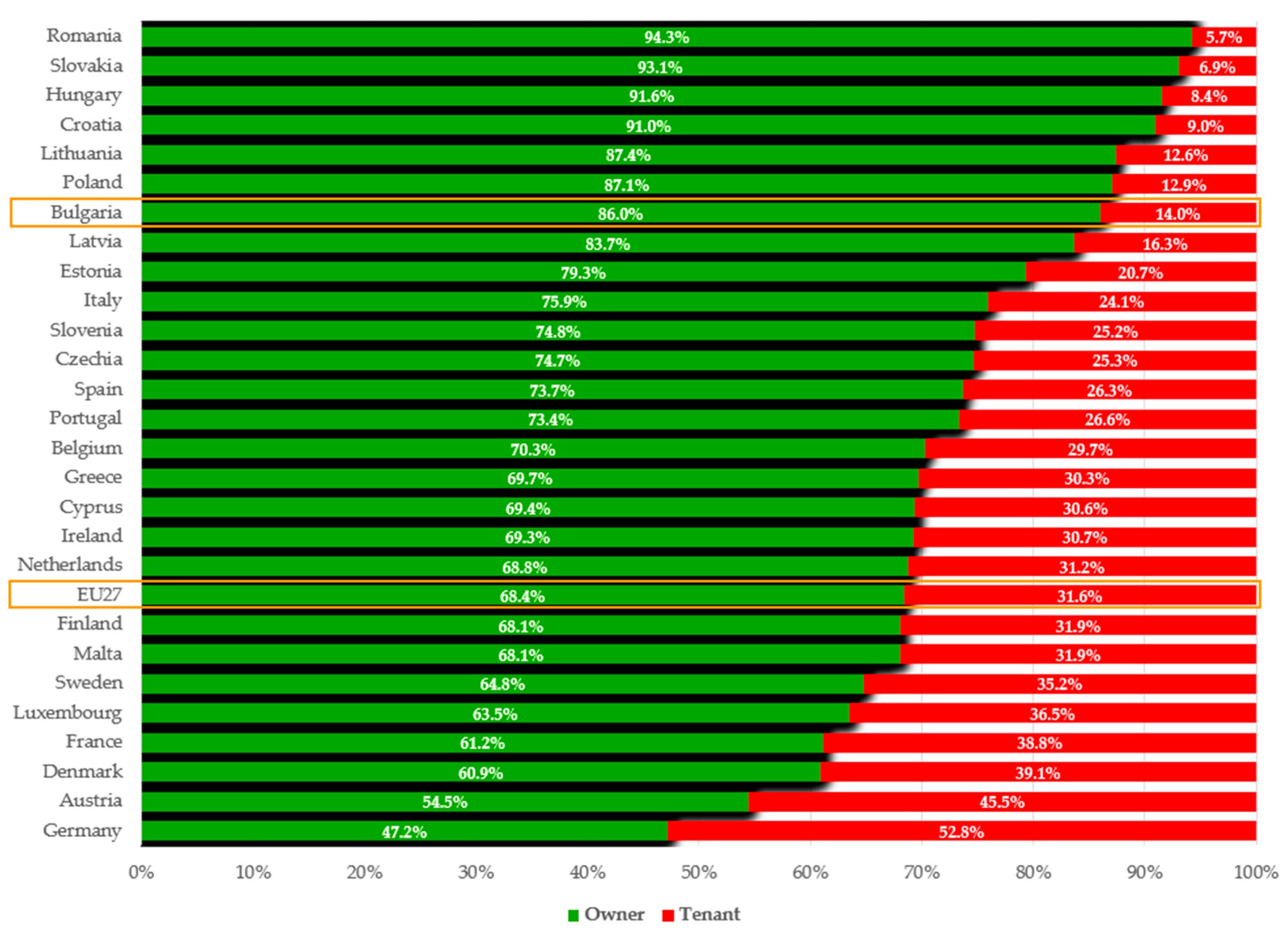
Figure 2.
EU countries HPI index change (2015=100): (a) Annual average rate of HPI change per countries and EU27; (b) Annual data of HPI per countries and EU27 for 2016, 2020 and 2024. Source: (Eurostat, 2025a), authors calculations and graphical illustration.
Figure 2.
EU countries HPI index change (2015=100): (a) Annual average rate of HPI change per countries and EU27; (b) Annual data of HPI per countries and EU27 for 2016, 2020 and 2024. Source: (Eurostat, 2025a), authors calculations and graphical illustration.
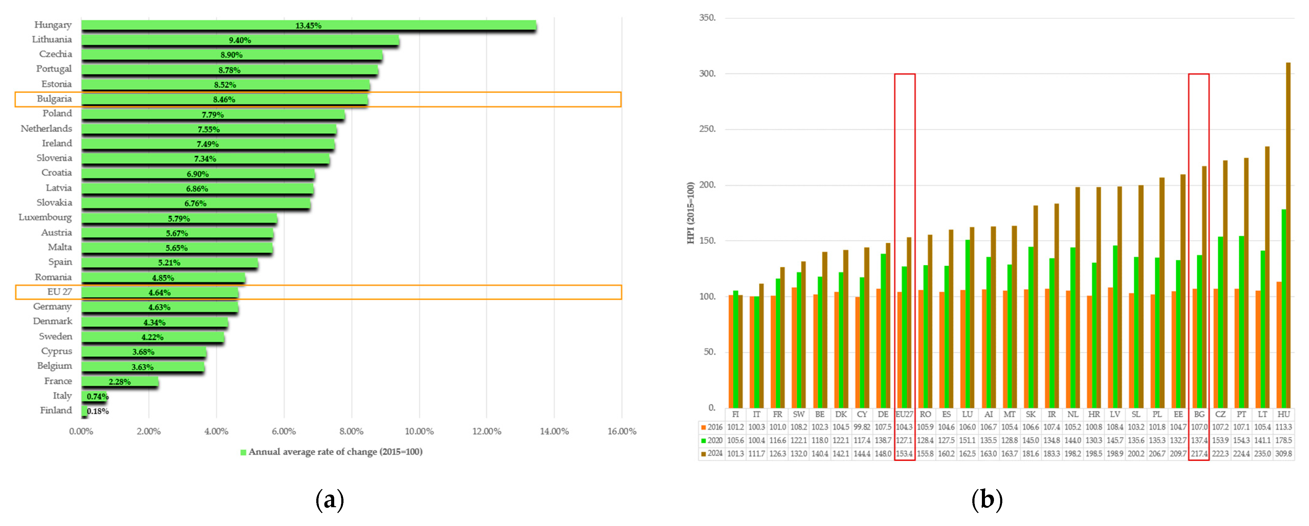
Figure 4.
Residual ACD and PACF distribution.
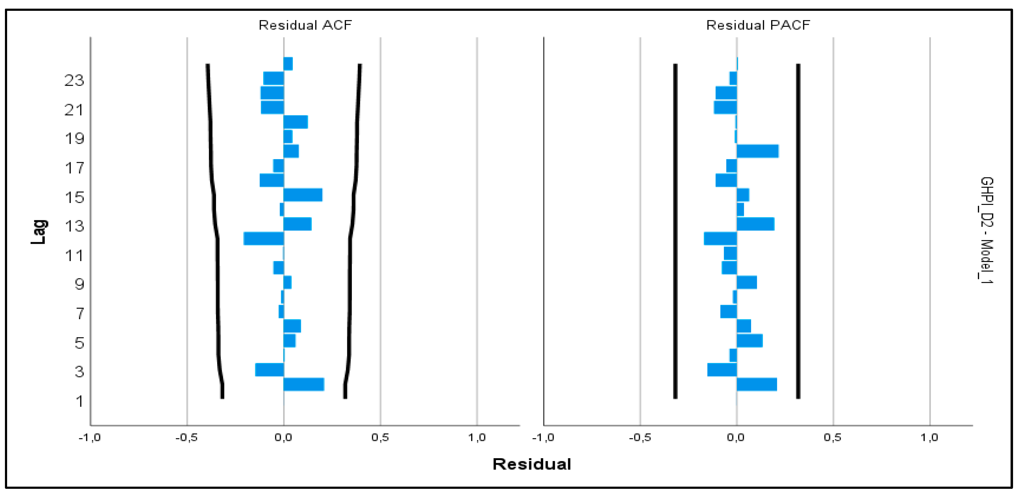
Table 1.
Test statistics.
| Descriptiona,b | GHPI |
| Kruskal-Wallis H | 0,353 |
| df | 3 |
| Asymp. Sig. | 0,950 |
a. Kruskal Wallis Test. b. Grouping Variable: Q.
Table 2.
ARIMAX (0,2,1) without кoнстанта.
| Model Description | |||
| Model Type | |||
| Model ID | GHPI_D2 | Model_1 | ARIMA(0,0,1)(0,0,0) |
Table 3.
Model Fit.
| Fit Statistic | Mean | SE | Minimum | Maximum | Percentile | ||||||
| 5 | 10 | 25 | 50 | 75 | 90 | 95 | |||||
| Stationary R-squared | 0,873 | . | 0,873 | 0,873 | 0,873 | 0,873 | 0,873 | 0,873 | 0,873 | 0,873 | 0,873 |
| R-squared | 0,873 | . | 0,873 | 0,873 | 0,873 | 0,873 | 0,873 | 0,873 | 0,873 | 0,873 | 0,873 |
| RMSE | 1,252 | . | 1,252 | 1,252 | 1,252 | 1,252 | 1,252 | 1,252 | 1,252 | 1,252 | 1,252 |
| MAPE | 94,722 | . | 94,72 | 94,722 | 94,722 | 94,722 | 94,722 | 94,722 | 94,722 | 94,722 | 94,722 |
| MaxAPE | 1017,26 | . | 1017,26 | 1017,26 | 1017,26 | 1017,26 | 1017,26 | 1017,26 | 1017,26 | 1017,26 | 1017,26 |
| MAE | 0,902 | . | 0,902 | 0,902 | 0,902 | 0,902 | 0,902 | 0,902 | 0,902 | 0,902 | 0,902 |
| MaxAE | 2,825 | . | 2,825 | 2,825 | 2,825 | 2,825 | 2,825 | 2,825 | 2,825 | 2,825 | 2,825 |
| Normalized BIC | 0,833 | . | 0,833 | 0,833 | 0,833 | 0,833 | 0,833 | 0,833 | 0,833 | 0,833 | 0,833 |
Table 4.
Model Statistics.
| Model | Number of Predictors | Model Fit statistics | Ljung-Box Q(18) | Number of Outliers | |||||||||
| Stationary R-squared | R-squared | RMSE | MAPE | MAE | MaxAPE | MaxAE | Normalized BIC | Statistics | DF | Sig. | |||
| GHPI_D2-Model_1 | 3 | 0,873 | 0,873 | 1,252 | 94,722 | ,902 | 1017,259 | 2,825 | 0,833 | 11,785 | 17 | 0,813 | 0 |
Table 5.
ARIMAX (0,2,1) Model Parameters.
| Estimate | SE | t | Sig. | |||||
| GHPI_D2-Model_1 | GHPI_D2 | No Transformation | MA | Lag 1 | 0,693 | 0,149 | 4,635 | 0,000*** |
| OOHE_D2 | No Transformation | Numerator | Lag 0 | 0,624 | 0,070 | 8,972 | 0,000*** | |
| WSMSRD_D2 | No Transformation | Numerator | Lag 0 | 0,171 | 0,058 | 2,947 | 0,006** | |
| ARH_D2 | No Transformation | Numerator | Lag 0 | 0,421 | 0,143 | 2,937 | 0,006** | |
***Significant at the 0.001 level; **Significant at the 0.01 level; *Significant at the 0.05 level.
Table 6.
ARCH effect test results.
| Variables Entered/Removeda | ||||||||||||||||||||||||||
| Model | Variables Entered | Variables Removed | Method | |||||||||||||||||||||||
| 1 | NResid_sc_Lag12, NResid_sc_Lag11, NResid_sc_Lag9, NResid_sc_Lag8, NResid_sc_Lag7, NResid_sc_Lag3, NResid_sc_Lag10, NResid_sc_Lag4, NResid_sc_Lag5, NResid_sc_Lag2, NResid_sc_Lag6, NResid_sc_Lag1b | . | Enter | |||||||||||||||||||||||
| a. Dependent Variable: NResid_sc; b. All requested variables entered. | ||||||||||||||||||||||||||
| Model | R | R Square | Adjusted R Square | Std. Error of the Estimate | Change Statistics | |||||||||||||||||||||
| R Square Change | F Change | df1 | df2 | Sig. F Change | ||||||||||||||||||||||
| 1 | 0,567c | 0,322 | -0,304 | 2,20574 | 0,322 | 0,514 | 12 | 13 | 0,871 | |||||||||||||||||
| c. Predictors: (Constant), NResid_sc_Lag12, NResid_sc_Lag11, NResid_sc_Lag9, NResid_sc_Lag8, NResid_sc_Lag7, NResid_sc_Lag3, NResid_sc_Lag10, NResid_sc_Lag4, NResid_sc_Lag5, NResid_sc_Lag2, NResid_sc_Lag6, NResid_sc_Lag1 | ||||||||||||||||||||||||||
| ANOVAa | ||||||||||||||||||||||||||
| Model | Sum of Squares | df | Mean Square | F | Sig. | |||||||||||||||||||||
| 1 | Regression | 30,010 | 12 | 2,501 | 0,514 | 0,871c | ||||||||||||||||||||
| Residual | 63,248 | 13 | 4,865 | |||||||||||||||||||||||
| Total | 93,258 | 25 | ||||||||||||||||||||||||
| Coefficientsa | ||||||||||||||||||||||||||
| Model | Unstandardized Coefficients | Standardized Coefficients | t | Sig. | 95,0% Confidence Interval for B | |||||||||||||||||||||
| B | Std. Error | Beta | Lower Bound | Upper Bound | ||||||||||||||||||||||
| 1 | (Constant) | 2,302 | 1,725 | 1,334 | ,205 | -1,425 | 6,029 | |||||||||||||||||||
| NResid_sc_Lag1 | -0,026 | ,310 | -,023 | -,083 | ,935 | -,696 | ,645 | |||||||||||||||||||
| NResid_sc_Lag2 | -0,244 | ,309 | -,215 | -,792 | ,443 | -,911 | ,423 | |||||||||||||||||||
| NResid_sc_Lag3 | -0,207 | ,294 | -,183 | -,704 | ,494 | -,842 | ,428 | |||||||||||||||||||
| NResid_sc_Lag4 | -0,307 | ,297 | -,273 | -1,033 | ,321 | -,950 | ,335 | |||||||||||||||||||
| NResid_sc_Lag5 | -0,122 | ,308 | -,108 | -,397 | ,698 | -,787 | ,543 | |||||||||||||||||||
| NResid_sc_Lag6 | 0,328 | ,308 | ,291 | 1,063 | ,307 | -,338 | ,994 | |||||||||||||||||||
| NResid_sc_Lag7 | -0,238 | ,317 | -,206 | -,752 | ,465 | -,923 | ,446 | |||||||||||||||||||
| NResid_sc_Lag8 | -0,010 | ,298 | -,009 | -,034 | ,973 | -,655 | ,634 | |||||||||||||||||||
| NResid_sc_Lag9 | -0,041 | ,293 | -,036 | -,140 | ,891 | -,675 | ,593 | |||||||||||||||||||
| NResid_sc_Lag10 | 0,097 | ,294 | ,085 | ,330 | ,747 | -,538 | ,732 | |||||||||||||||||||
| NResid_sc_Lag11 | -0,094 | ,244 | -,105 | -,386 | ,706 | -,622 | ,434 | |||||||||||||||||||
| NResid_sc_Lag12 | -0,127 | ,237 | -,143 | -,537 | ,600 | -,640 | ,385 | |||||||||||||||||||
Disclaimer/Publisher’s Note: The statements, opinions and data contained in all publications are solely those of the individual author(s) and contributor(s) and not of MDPI and/or the editor(s). MDPI and/or the editor(s) disclaim responsibility for any injury to people or property resulting from any ideas, methods, instructions or products referred to in the content. |
© 2026 by the authors. Licensee MDPI, Basel, Switzerland. This article is an open access article distributed under the terms and conditions of the Creative Commons Attribution (CC BY) license (http://creativecommons.org/licenses/by/4.0/).
Copyright: This open access article is published under a Creative Commons CC BY 4.0 license, which permit the free download, distribution, and reuse, provided that the author and preprint are cited in any reuse.


