
Submitted:
25 February 2026
Posted:
26 February 2026
You are already at the latest version
Abstract
Handling missing data is a central challenge in quantitative research, particularly when datasets exhibit complex dependency structures, such as nonlinear relationships and interactions. Multiple imputation (MI) via fully conditional specification (FCS), as implemented in the mice R package, is widely used but relies on user-specified models that may fail to capture complex dependency structures, especially in high-dimensional settings, or on more sophisticated algorithms that are considered data-hungry. This paper investigates the performance of TabPFN, a transformer-based, pretrained foundation model developed for tabular prediction tasks, for MI. TabPFN is pretrained on millions of synthetic datasets and approximates posterior predictive distributions without dataset-specific retraining, offering a compelling solution for imputing complex missing data in small to moderately sized samples. We conduct a simulation study focusing on univariate missingness in a continuous outcome, comparing TabPFN with standard MI methods. Performance is evaluated using bias, standard error, and coverage of the marginal mean estimand across a range of data-generating - and missingness mechanisms. Our results show that TabPFN yields competitive or superior performance relative to classification and regression trees and predictive mean matching. These findings highlight TabPFN as a promising new tool for missing data imputation, with particular relevance to health research.
Keywords:
missing data
; multiple imputation
; TabPFN
; pretrained models
; in-context learning
; simulation study
; complex dependency structures
1. Introduction
Quantitative analyses in health research, including clinical trials and observational studies, commonly assume that all variables are fully observed. In practice, however, missing data in covariates or outcomes are ubiquitous and, if not appropriately handled, can lead to biased estimates, loss of efficiency, and invalid statistical inference [1,2]. Regulatory guidance therefore, emphasizes the need for principled approaches to missing data that support valid estimation and uncertainty quantification, particularly for prespecified estimands in confirmatory analyses. Multiple imputation (MI) provides a widely accepted framework for addressing missing data under valid uncertainty quantification by generating multiple plausible completed datasets, analyzing each dataset separately, and combining results using Rubin’s rules to reflect both sampling variability and uncertainty due to missingness [3].
The performance of MI depends critically on the adequacy of the imputation models used to approximate the joint distribution of the data. When important complex dependency structures, such as nonlinear relationships or interactions, are omitted from the imputation models, MI can yield biased point estimates and misleading measures of uncertainty [4,5]. This challenge is particularly relevant when several variables are partially observed, a setting commonly addressed using fully conditional specification (FCS) algorithms, such as those implemented in the widely used mice (Multivariate Imputation by Chained Equations) R package [6]. FCS MI proceeds by iteratively imputing each incomplete variable using a univariate conditional model given the current values of all other variables. While this framework is flexible and has proven effective in many applied settings, it requires careful specification of functional forms, transformations, and interactions in each conditional model to ensure compatibility with the substantive analysis model. This task becomes increasingly challenging in high-dimensional settings or when relationships between variables exhibit complex dependency structures [7].
Motivated by these challenges, a growing body of research has explored the use of flexible predictive algorithms for missing data imputation. Tree-based methods such as classification and regression trees (CART) [8], random forests [9], and gradient boosting approaches including XGBoost [10] have been incorporated into imputation frameworks such as mice and mixgb. Simulation studies suggest that these approaches can better preserve complex dependency structures than traditional parametric imputation models, leading to improved finite-sample performance in some settings [11,12,13,14]. Related work includes ensemble-based MI using super learners, as implemented in the misl package [15], and MI based on multivariate adaptive regression splines (MARS), which have demonstrated favorable confidence interval coverage under complex data-generating mechanisms [16].
Despite these advances, highly flexible models typically require substantial sample sizes to reliably estimate complex dependency structures [17,18]. While large observational datasets may support such approaches, clinical trials and other confirmatory studies are often limited in size, making it difficult to estimate complex imputation models without imposing strong structural assumptions. Nevertheless, appropriately addressing missing data remains essential for maintaining valid statistical inference in these settings, particularly when regulatory decisions depend on accurate estimation and uncertainty quantification [19].
Recent developments in foundation models for tabular data offer a promising alternative to conventional task-specific modeling approaches, which often struggle to generalize under limited data settings [20]. The Tabular Prior-Data Fitted Network (TabPFN), introduced by Hollmann et al. [21], is a transformer-based model trained on millions of synthetic tabular datasets. By learning a broad prior over data-generating processes, TabPFN is designed to generalize across a wide range of prediction tasks, effectively encoding structural assumptions learned during pretraining rather than relying solely on estimation from the observed data. Even without task-specific fine-tuning, TabPFN has demonstrated strong predictive performance in small to moderately sized datasets (up to approximately 10’000 observations and 500 features) [22,23] making TabPFN particularly attractive for data-scarce domains [23].
Naturally, promising prediction algorithms are adapted for missing data imputation tasks often in the context of single imputation (SI), where missing values are replaced by a single predicted value, as in the TabPFN-based imputation approach proposed by Feitelberg et al. [24], which is specifically pretrained for imputing missing values. While such SI approaches may perform well in terms of predictive accuracy, strong predictive performance alone does not guarantee valid statistical inference after imputation. SI does not propagate uncertainty due to missingness and therefore generally yields overly optimistic standard errors and confidence intervals [1]. Because of this inadequate uncertainty quantification, MI is generally recommended over SI for inferential purposes [19,25]. To date, the use of pretrained foundation models such as TabPFN within a MI framework explicitly designed to preserve inferential validity remains largely unexplored.
The aim of this paper is to investigate the performance of TabPFN as an imputation engine within a MI framework suitable for valid statistical inference. Our contributions are threefold. First, we propose a principled integration of TabPFN into an MI procedure that explicitly accounts for uncertainty due to missing data. Second, we conduct an extensive simulation study to compare the proposed approach with established MI methods implemented in mice, focusing on bias, standard error, and confidence interval coverage under a range of data-generating and missingness mechanisms. Third, we illustrate the practical relevance of the method using a real-data example motivated by applied epidemiological research. Section 2 introduces the TabPFN model and its use for MI. Section 3 describes the simulation design, competing methods, and evaluation metrics. Section 4 presents the simulation results, Section 5 provides a real-data application, and Section 6 concludes with a discussion of implications and directions for future research.
2. Methods
2.1. Brief Introduction to TabPFN
TabPFN is a transformer-based neural network architecture incorporating self-attention mechanisms [26], originally developed for sequence modeling in natural language processing and later extended to various other domains, including tabular data. TabPFN is designed for classification and regression tasks and aims to approximate predictive distributions induced by a broad prior over data-generating processes in a nonparametric and computationally efficient manner [27].
Unlike traditional models that must be retrained for each new dataset, TabPFN is pretrained on a wide range of synthetic datasets. These datasets are generated by sampling from a distribution over a variety of data-generating processes, including structural causal models and Bayesian neural networks with varying parameters and noise levels [28]. This distribution of data-generating processes – referred to by the authors as the prior – is designed to favor parsimonious structures while still encompassing a broad spectrum of realistic relationships commonly encountered in applied data analysis. Through this pretraining, TabPFN learns to approximate predictive distributions across diverse data scenarios without requiring dataset-specific retraining.
For a specific task, TabPFN is provided with complete cases, consisting of observed outcomes and covariates , and incomplete cases, with observed covariates but missing outcomes . A single forward pass through the pretrained model yields a predictive distribution for that reflects both the observed data and the prior assumptions [21].
In practice, TabPFN has been shown to support efficient predictive inference on small-to-moderately sized datasets (e.g., up to approximately 10’000 observations on GPU or 1’000 observations on CPU with hundreds of variables), as reported in Hollmann et al. [21], making it particularly well suited to experimental settings where data collection is costly. TabPFN’s output is a full predictive distribution rather than a single point estimate, from which MIs can be generated by repeated sampling. Hence, MIs are obtained by independently sampling from this predictive distribution for each missing value, thereby introducing stochastic variation across imputations conditional on the observed data. Because the model is pretrained on a diverse range of generative processes, it can capture complex structures such as nonlinear associations, variable interactions, and heteroskedasticity. These features make TabPFN a promising method for handling missing data in biomedical and epidemiological research, where such complexities and limited sample sizes often challenge more traditional imputation methods.
2.2. Using TabPFN for Multiple Imputation
Focusing on univariate missingness, we defined as the partially missing outcome variable, with corresponding predictors that were fully observed. The missingness indicator vector was denoted by M, where indicated that was missing and indicated that was observed. Thus, and represent the observed subset of Y and (i.e., where ), while and represent the subset with missing Y (i.e., where ).
Missing data mechanisms are commonly classified as missing completely at random (MCAR), when the probability of missingness is independent of both observed and unobserved data; missing at random (MAR), when it depends only on observed data; and missing not at random (MNAR), when it depends on unobserved information such as the partially missing variable Y itself. Here, we focus on imputation under MAR (or MCAR).
TabPFN performs classification. Therefore, continuous outcomes are discretized into a fixed number of classes prior to imputation, effectively reframing the regression problem as a multi-class classification task. For each observation with , TabPFN outputs a vector of class probabilities, representing a predictive distribution for conditional on , , and . This discretization constitutes an approximation to the underlying continuous outcome distribution and may affect variance estimation and tail behavior. Its impact on inferential performance is therefore evaluated empirically in the simulation study.
Thus, under the MAR (or MCAR) assumption, when all variables driving the missingness mechanism are observed and included in the imputation model, MIs can be generated by sampling from these discrete predictive distributions without specifying a parametric error distribution. For additional details, including feature pre-processing, acceleration, and post-hoc ensembling, we refer to Hollmann et al. [21].
We do not claim formal theoretical validity of Rubin’s rules under TabPFN-based imputation. Instead, inferential adequacy of the proposed approach is evaluated empirically through bias, standard error behavior, and confidence interval coverage in controlled simulation settings. Rubin’s rules are applied under the working assumption that TabPFN’s predictive draws approximate proper posterior predictive distributions for the missing values, such that between-imputation variability reflects uncertainty about the missing data.
3. Simulation Study
The simulation setup employed in this study was closely aligned with a design previously used by Sepin [16], which itself builds upon the second simulation study by Little and An [29]. The design varied sample size, number of noise variables, outcome structure, and missingness mechanism, resulting in a fully factorial set of scenarios. All simulations were implemented in R using GPU acceleration.
In line with the recommendation by Oberman and Vink [30], we used the same simulated dataset across all strategies within each simulation run to eliminate unnecessary variation and ensure fair comparison.
3.1. Data and Missingness Generation
We considered a single partially observed outcome Y, with the estimand of interest being the marginal mean . The covariates available for the missing data imputation consisted of two informative predictors along with two different amounts of irrelevant noise variables. For each simulation run, we independently generated n observations according to the following data-generating process. Two covariates relevant for the outcome and missingness mechanisms, and , were generated as independent draws from the uniform distribution on . In addition, p irrelevant noise variables were independently sampled from a standard normal distribution, .
The outcome Y was then generated as a function of and , according to one of three structural forms:
- Linear:
- Additive:
- Non-additive:
which means that each structure implies a marginal mean of . Missingness in Y was imposed under both MCAR and MAR mechanisms with approximately 50% missingness. The probability of observing Y, conditional on and , was defined as follows:
- MCAR:
- Linear MAR:
- Additive MAR:
- Non-additive MAR:
where . Investigating behavior under MNAR mechanisms was outside the scope of this study. In total, the simulation design formed a full factorial combination of:
- : number of noise variables
- : number of observations
- 3 mean structures: linear, additive, non-additive
- 4 missingness mechanisms: MCAR, linear MAR, additive MAR, non-additive MAR
resulting in 72 experimental conditions each repeated 250 times.
3.2. Performance Evaluation
Let denote the pooled estimate of obtained via Rubin’s rules after MI in simulation repetition , where . To assess the performance of each MI method, we computed the following summary statistics across simulation runs:
-
Mean and Standard Deviation of Bias:For each simulation repetition, the bias was defined as . For each method and simulation condition, we reported the mean and standard deviation of the resulting biases.
-
Mean and Standard Deviation of the Standard Error (SE):The within-imputation standard error of , denoted by , was calculated and summarized using the mean and standard deviation across repetitions.
-
Coverage of the 95% Confidence Interval:To assess interval performance, we evaluated whether 10 fell within the 95% confidence interval for . Specifically, we checked whether where denotes the percentile of the t-distribution with pooled degrees of freedom according to Barnard and Rubin [31]. Coverage was then defined as the proportion of simulations in which this criterion was met.
Uncertainty in the estimated 95% coverage rate was quantified using a 90% Wilson confidence interval. Finally, for each method and condition, we recorded the average computation time required to complete the imputation and pooling process.
3.3. Secondary Simulation: Sensitivity to the Number of Imputations (m)
To assess the sensitivity of our findings to the number of imputations, we conducted a secondary simulation study varying the number of imputed datasets (m). Specifically, we re-ran the simulation scenarios with a non-additive outcome structure at the smallest sample size () using imputations and compared the results to those obtained with the default choice of . All missingness mechanisms (constant, linear, additive, and non-additive) and noise variables () considered in the primary simulation study were retained.
This specific scenario was chosen since the metric was comparatively high (see Figure A1 in the Appendix), where B denotes the between-imputation variance and T the total variance of the MI estimator. can be interpreted as the proportion of the variation attributable to the missing data and thus reflects the difficulty of the imputation problem. Values close to zero indicate that the contribution of missingness to the overall variance is negligible, a situation that can only arise if the missing values can be recovered almost perfectly. Conversely, values near one indicate that uncertainty is dominated by missing data, corresponding to situations in which the observed data contain little information about the missing values [32] Chapter 2.3.5. Increasing the number of imputations m provides an additional lever for stabilizing inference and is therefore sometimes used to guide the choice of m in practice [32] Chapter 2.8.
Across all scenarios, estimates of the performance metrics were very similar for and with no qualitative changes in method ranking or conclusions, suggesting that imputations are sufficient for the scenarios considered here. Detailed results are provided in Figure A2 in the Appendix.
4. Results
We conducted a simulation study, broadly following the principles outlined in Little and An [29] and Sepin [16], to compare the performance of TabPFN-based MI with established MI methods. All MI procedures produced complete datasets with no remaining missing values.
Figure 1 shows the bias of estimates, with error bars representing the 25th, 50th (median), and 75th percentiles, with mean and standard deviation reported in parentheses. Bias was defined as the difference between each method’s pooled estimate and the true parameter value of 10. Complete-case (CC) analysis, which omits all observations with missing values, was included as a baseline. Across most experimental settings, CC produced the largest deviations from the true value (except under MCAR), underscoring the inefficiency of discarding incomplete cases. In contrast, MI methods yielded pooled estimates closer to the full-data estimand computed before introducing missingness, substantially reducing bias induced by missingness. Among the MI approaches considered, TabPFN-based MI exhibited among the smallest biases across simulation scenarios. Increasing the sample size generally reduced bias, while reducing the number of noise variables had a smaller but still favorable effect. PMM, which relies on linear and additive conditional models, showed limited bias reduction with increasing sample size when these assumptions were violated, whereas the more flexible CART and TabPFN approaches benefited from larger samples in such settings. Similarly, under MCAR (constant missingness), PMM produced notably biased estimates for non-linear mean structures (additive and non-additive) when many noise variables were present, whereas CART and TabPFN adapted effectively.
Figure 2 shows the standard errors (SEs) of estimates, with error bars representing the 25th, 50th (median), and 75th percentiles, with mean and standard deviation reported in parentheses. The red vertical lines indicate the median standard errors from the full-data analysis (before introducing missingness), serving as reference values. As expected, in most scenarios MI methods had larger SEs than the full-data SE, reflecting the inclusion of both within- and between-imputation variance. In the most challenging scenarios involving non-additive missingness, TabPFN occasionally produced standard errors slightly smaller than the full-data reference, suggesting mild underestimation of uncertainty in finite samples. CART-based imputations tend to underestimate uncertainty and do not satisfy the conditions for proper MI unless additional stochasticity (e.g., bootstrap resampling) is introduced, as discussed in the MI literature (e.g. van Buuren [32] [Chapter 3.5]). PMM generally yielded larger and more conservative standard errors. Increasing the sample size reduced SEs, while adding noise variables generally increased them. Performance under MCAR (constant missingness) showed similar behavior.
Coverage rates for 95% confidence intervals (CIs) are shown in Figure 3. Ideally, coverage should be close to 95%. Several methods failed to attain nominal coverage in specific scenarios, indicating underestimation of uncertainty even under MCAR missingness. Larger sample sizes generally improved coverage. However, for methods with restrictive modeling assumptions, such as PMM and CC, coverage sometimes deteriorated when these assumptions were violated by the data-generating mechanism. In some cases, inflated SEs produced conservative coverage, though at the expense of precision. The TabPFN-based MI approach maintained coverage close to the nominal 95% level across most scenarios, with undercoverage primarily observed for the combination of non-additive mean structure and non-additive missingness at the smallest sample size ().
Average computational times to generate imputations are given in Table 1. The whole simulation study was executed in Google Colab using an A100 GPU and took approximately 92 hours in total to run. TabPFN required substantially longer computation times than competing methods. Moreover, practical use of TabPFN currently depends on access to specialized hardware, such as GPUs, which may limit its applicability in some settings.
5. Case Study: Estimating the Effect of Smoking Cessation on Weight Gain
We revisit a classic benchmark example from What If? [33], which investigates the causal effect of smoking cessation on weight gain using data from the National Health and Nutrition Examination Survey Epidemiologic Follow-Up Study (NHEFS). The data and original analysis code are publicly available from the book’s website (https://miguelhernan.org/whatifbook). The case study is intended to illustrate practical differences between imputation strategies rather than to establish a causal ground truth.
The cohort consists of 1’566 adult smokers aged 25–74 who completed both a baseline visit (1971–1975) and a follow-up visit approximately 10 years later. Smoking status was assessed at both visits, and individuals were classified as quitters () if they had quit smoking before follow-up, or as non-quitters () otherwise. The outcome of interest, weight gain (Y), was defined as the difference in measured weight (kg) between the two visits.
We follow the approach outlined in Westreich et al. [34], leveraging MI approaches to estimate the average causal effect (ACE) of smoking cessation on weight gain,
where and denote the potential weight gains had all individuals quit or not quit smoking, respectively. Identification of the ACE relies on the standard assumptions of consistency, conditional exchangeability given measured baseline covariates, and positivity. As in Hernán and Robins [33] [Chapter 13], we assume that the available baseline covariates are sufficient to control for confounding.
Because each individual is observed under only one treatment condition, the counterfactual outcome under the alternative condition is unobserved. This structure allows causal inference to be formulated as a missing-data problem in which the missingness mechanism corresponds to treatment assignment. However, valid inference still depends on appropriate modeling of the outcome conditional on covariates and treatment.
Hernán and Robins estimate the ACE using g-computation based on a linear outcome regression model. Specifically, the observed outcome is modeled as
where indicates smoking cessation, demographic variables include sex, race, age, and education, smoking history is summarized by smoking intensity and smoking years, physical activity is captured by exercise and activity indicators, and denotes baseline weight. In addition to the variables used in Equation 2, the NHEFS dataset contains further baseline covariates describing socioeconomic status, health behaviors, and clinical characteristics, which we later exploit in the imputation models (see Table A1 in the Appendix).
In the original analysis, Equation 2 is used for g-computation. Briefly, g-computation fits the outcome model and predicts each individual’s potential outcomes under both treatment conditions by setting and , while holding all other covariates fixed. This yields predicted potential outcomes and for each individual. The ACE is computed as the mean difference between these two predictions across individuals (), with uncertainty quantified via nonparametric bootstrap (500 resamples). Because both observed and counterfactual outcomes are replaced by model predictions, the resulting estimate depends entirely on the correctness of the specified outcome model.
In contrast, the MI approach leaves the observed outcomes unchanged and imputes only the missing counterfactual outcomes, treating them explicitly as missing data. This distinction means that observed data retain their original variability, and model uncertainty is propagated through MI. To reflect a realistic setting where the true outcome model is unknown, we extend the imputation model to include a richer set of 46 covariates from NHEFS. To isolate the impact of imputation methods on counterfactual outcomes only, we restrict attention to individuals with complete baseline covariate information, yielding a final analytic sample of 490 individuals for all analyses (see Table A1 in the Appendix).
The dataset is then restructured so that each individual has two records, one per treatment condition, with weight gain observed for the factual treatment and imputed for the counterfactual. We generate 100 imputations and pool results using Rubin’s rules.
Table 2 presents ACE estimates, standard errors, and 95% confidence intervals based on normal approximation. The g-computation estimate was 3.380 kg, closely matching the result reported in Hernán and Robins [33] [Chapter 13]. CART yields an ACE estimate of similar magnitude (3.419 kg), whereas TabPFN produces a somewhat lower estimate (2.746 kg), and PMM obtained the smallest effect estimate (2.363 kg).
Because the true causal effect is unknown in observational data, it is not possible to determine which estimate is closest to the truth. All 95% confidence intervals overlapped, indicating no clear contradiction across methods. The differences in point estimates likely reflect the distinct modeling assumptions underlying the approaches. PMM and g-computation rely on analyst-specified linear models and therefore impose stronger functional form constraints: in PMM, the imputation model is linear and additive, with flexibility arising only indirectly through donor selection, whereas g-computation explicitly incorporates selected nonlinear terms and interactions as specified in Equation 2. In contrast, CART and TabPFN adapt more flexibly to complex covariate structures, with CART being fully data-driven and TabPFN incorporating regularization through its pretrained prior, which may shrink extreme counterfactual predictions toward more conservative values.
6. Discussion
Flexible, nonparametric approaches such as CART and random forests have repeatedly been shown to reduce bias under complex dependency structures, particularly when linearity and additivity assumptions are violated [11,12,13], with recent work using XGBoost pushing performance even further [14]. However, these methods typically require moderate to large sample sizes to estimate such structures reliably, posing challenges in applied settings with limited data availability [18,20]. Our findings suggest that pretrained, foundation-model–style predictors such as TabPFN may partially alleviate this gap in small-sample settings by leveraging strong prior information learned from large collections of synthetic datasets. By introducing and benchmarking a TabPFN-based MI algorithm, we show that it achieves performance that is comparable to, and in some scenarios superior to, standard MI methods with minimal model specification effort, potentially mitigating one of the key limitations of highly flexible approaches in low-sample settings.
The strong performance of TabPFN-based MI likely reflects its ability to approximate complex dependency structures without requiring explicit specification of functional forms or interactions in the imputation model. PMM relies on linear predictive models to define donor pools for matching and is therefore more robust than fully parametric imputation with respect to outcome distributional assumptions, while remaining sensitive to misspecification of the conditional mean structure [7,35]. TabPFN, on the other hand, was able to adapt across data structures, similar to findings for other tree-based or ensemble methods [13]. While CART also benefited from model flexibility, it has a tendency to underestimate uncertainty because CART-based imputation models, as implemented in mice, are typically fitted without bootstrap resampling. This results in insufficient between-imputation variability and renders the procedure formally improper under standard MI theory, as documented in the MI literature [32] [Chapter 3.5] and also observed in our simulations. Overall, TabPFN achieved lower bias and more reliable coverage than competing methods, even at smaller sample sizes.
Several limitations warrant consideration. Our simulation study focused on univariate missingness in a continuous outcome with continuous predictors. Many real-world datasets include multivariate missingness and mixed data types, which pose additional challenges. TabPFN provides an unsupervised prediction mode, but this mode currently yields deterministic predictions rather than draws from a well-defined posterior predictive distribution. This may underestimate variability in subsequent analyses, potentially leading to anti-conservative inference and inflated Type I error rates, a well-known consequence of single or insufficiently stochastic imputation [2,3] [Chapter 1.5, Chapter 4]. Although MI is designed to propagate uncertainty due to missingness, its validity depends critically on the adequacy of the underlying imputation models. Biased, poorly calibrated, or overly deterministic imputation mechanisms can counteract the theoretical advantages of MI, particularly in complex or low-sample settings. While TabPFN improved performance in many scenarios, it did not achieve nominal properties in all settings, particularly under the most challenging combinations of non-additive mean structure and non-additive missingness. Further methodological development is therefore required to improve robustness and theoretical foundation across a broader range of settings.
Because TabPFN is pretrained exclusively on synthetically generated datasets, evaluation based solely on synthetic simulation studies may raise concerns about potential over-optimism if the synthetic pretraining distribution overlaps substantially with the data-generating mechanisms used for evaluation. In line with Murray [36] and Oberman and Vink [30], we advocate for unified evaluations of MI methods combining controlled simulations with results from publicly available benchmark datasets, similar to TabArena in prediction research [22] or RealCause in causal inference from observational data [37], to ensure fair and transparent comparisons.
Finally, TabPFN is computationally more demanding than simpler MI methods such as PMM or CART. While access to GPU resources is increasingly common in research environments and unlikely to be prohibitive relative to the overall cost of large studies, the additional computational and software complexity may nevertheless pose practical barriers for routine use in standard statistical workflows. These considerations are particularly relevant for analysts accustomed to lightweight, CPU-based MI implementations. Moreover, TabPFN’s relative novelty means it has not yet been extensively tested across diverse applied contexts. Even though adoption in the Healthcare and Life Sciences section is strongest [23], adoption in regulatory contexts where transparency, reproducibility, and extensive methodological validation are emphasized, may be more gradual [1,19].
TabPFN-based MI represents a promising addition to the MI toolkit and illustrates the broader potential of foundation-model–based approaches for missing data imputation, particularly in limited-data settings where traditional imputation models struggle and expert knowledge about functional relationships is limited or unavailable. Its ability to combine modeling flexibility with generally robust coverage properties makes it a promising candidate for further application in the missing data imputation area. Importantly, TabPFN is not the only foundation model with potential for MI, and the area of foundation-model–based imputation is developing rapidly, with new architectures and training strategies continually emerging. Future research should focus on improving computational efficiency to facilitate broader adoption, potentially through domain-specific or lightweight variants, and on systematic benchmarking against both established MI methods and alternative foundation-model approaches to better characterize the relative strengths and limitations of these models.
Supplementary Materials
The following supporting information can be downloaded at the website of this paper posted on Preprints.org.
Funding
This research received no external funding.
Institutional Review Board Statement
Not applicable.
Informed Consent Statement
Not applicable.
Data Availability Statement
All material to reproduce the results is available in the supplementary materials.
Acknowledgments
I would like to thank Prof. Dr. Stefan Boes for valuable discussions and feedback.
Conflicts of Interest
The author declares no competing interests.
Appendix A
Figure A1.
Proportion of the variation attributable to the missing data (). Values close to zero indicate that the contribution of missingness to the overall variance is negligible (perfect recovery of missing observations). Values near one indicate that uncertainty is dominated by missing data, corresponding to situations in which the observed data contain little information about the missing values.
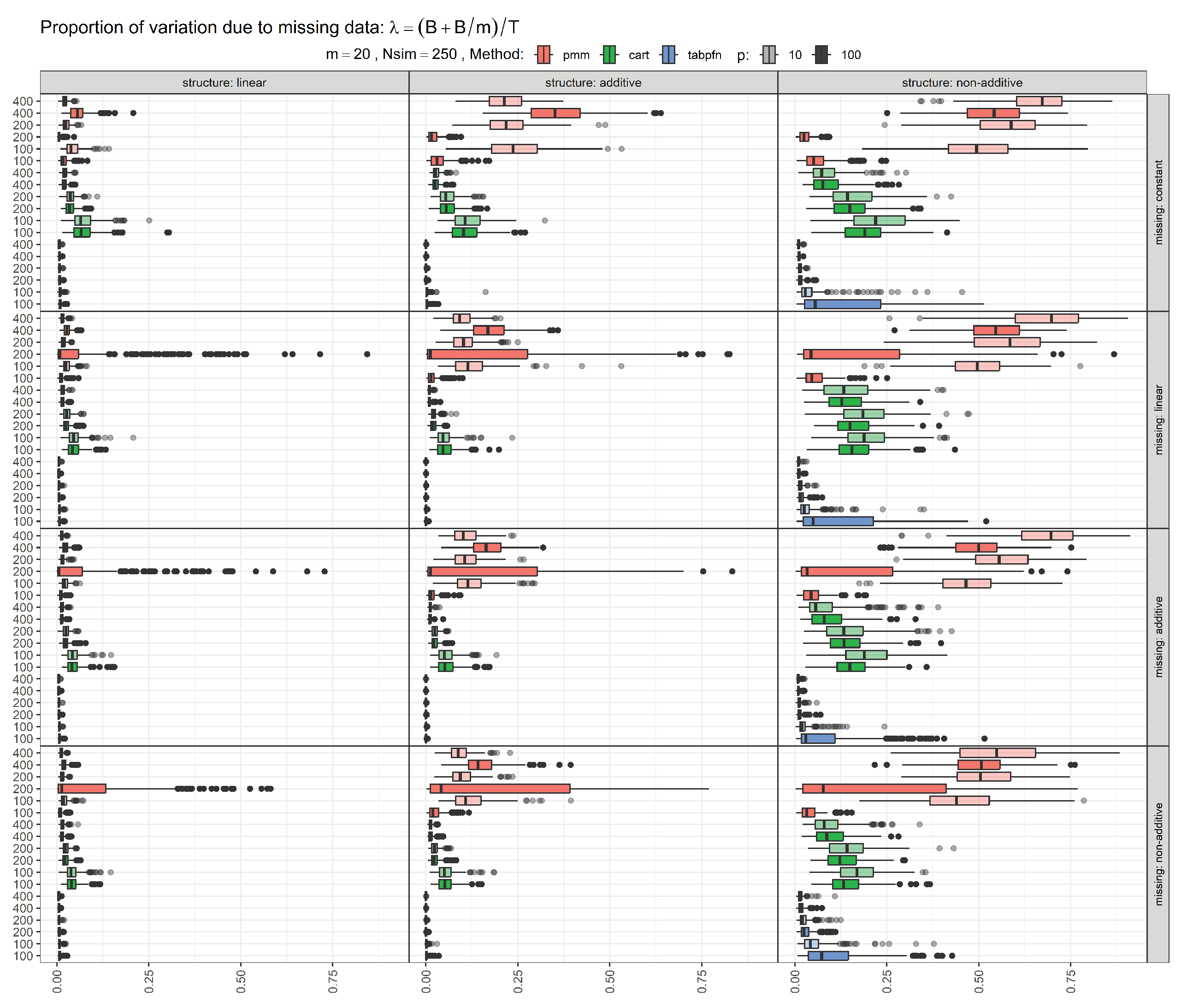
Figure A2.
Sensitivity to the number of imputations: performance metrics remain stable when increasing m from 20 to 100.
Figure A2.
Sensitivity to the number of imputations: performance metrics remain stable when increasing m from 20 to 100.
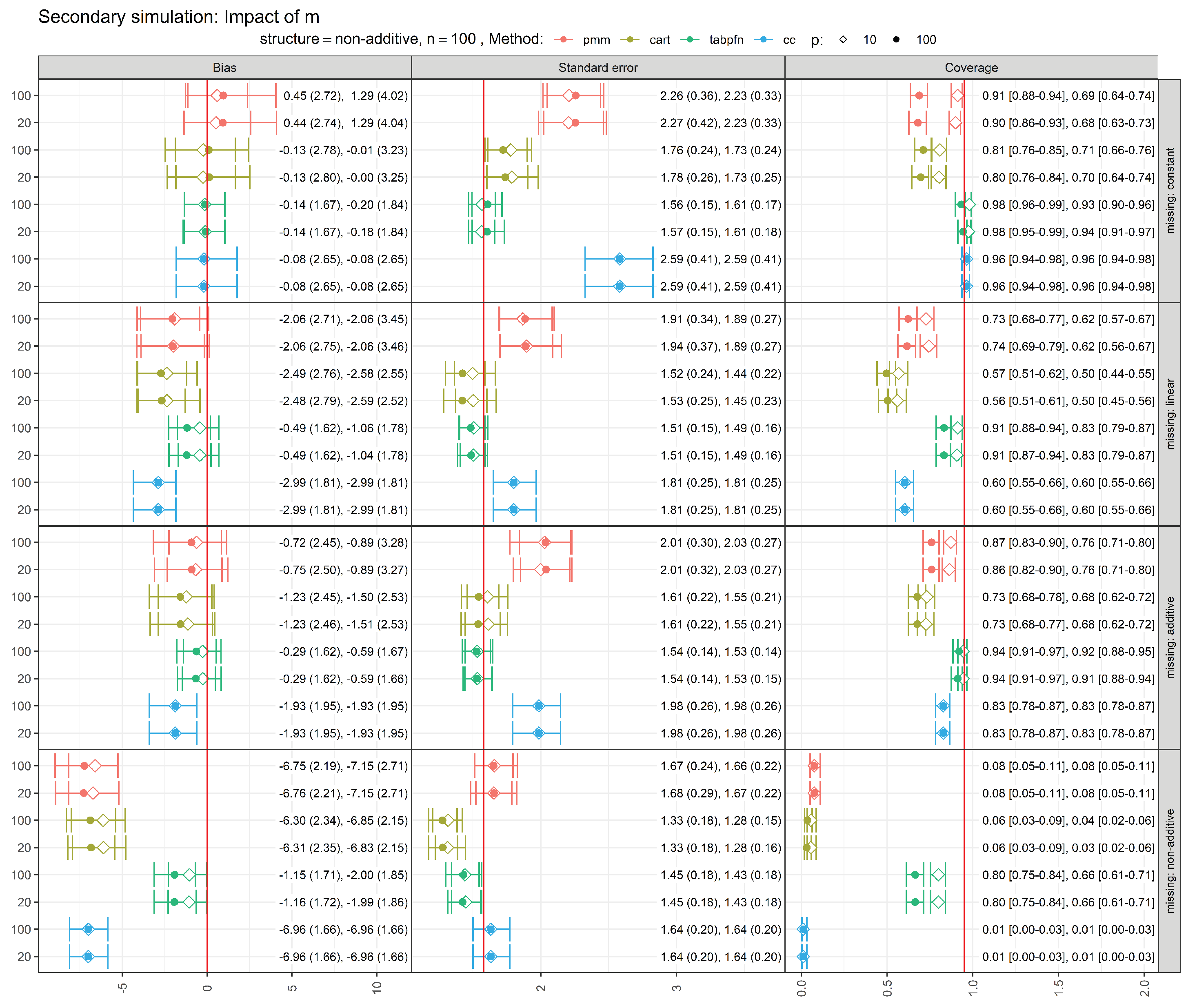

Table A1.
Description of NHEFS cohort with missing observations removed.
| Stratified by smoking | Non-quitters | quitters |
|---|---|---|
| n | 363 | 127 |
| Weight change [kg] (mean (SD)) | 2.09 (7.43) | 4.54 (8.68) |
| Weight in 1971 [kg] (mean (SD)) | 72.30 (14.67) | 74.41 (14.46) |
| Sex = Male (%) | 205 (56.5) | 80 (63.0) |
| Race = White (%) | 304 (83.7) | 113 (89.0) |
| Age in 1971 (mean (SD)) | 42.50 (11.95) | 46.06 (12.67) |
| Amount of education (%) | ||
| 8th grade or less | 58 (16.0) | 23 (18.1) |
| College dropout | 22 (6.1) | 12 (9.4) |
| College or more | 36 (9.9) | 20 (15.7) |
| Highschool | 161 (44.4) | 53 (41.7) |
| Highschool dropout | 86 (23.7) | 19 (15.0) |
| Number of cigarettes smoked per day (mean (SD)) | 20.73 (11.26) | 17.86 (12.27) |
| Years of smoking (mean (SD)) | 23.94 (11.99) | 25.49 (13.57) |
| In recreation, how much exercise? (%) | ||
| little or no exercise | 142 (39.1) | 61 (48.0) |
| moderate exercise | 137 (37.7) | 46 (36.2) |
| much exercise | 84 (23.1) | 20 (15.7) |
| In your usual day, how active are you? (%) | ||
| inactive | 29 (8.0) | 9 (7.1) |
| moderately active | 145 (39.9) | 56 (44.1) |
| very active | 189 (52.1) | 62 (48.8) |
| Total family income [USD] (%) | ||
| <1000 | 3 (0.8) | 2 (1.6) |
| 1000-1999 | 16 (4.4) | 2 (1.6) |
| 10000-14999 | 90 (24.8) | 41 (32.3) |
| 15000-19999 | 54 (14.9) | 17 (13.4) |
| 2000-2999 | 17 (4.7) | 3 (2.4) |
| 20000-24999 | 26 (7.2) | 6 (4.7) |
| 25000+ | 15 (4.1) | 7 (5.5) |
| 3000-3999 | 11 (3.0) | 7 (5.5) |
| 4000-4999 | 15 (4.1) | 3 (2.4) |
| 5000-5999 | 15 (4.1) | 3 (2.4) |
| 6000-6999 | 12 (3.3) | 3 (2.4) |
| 7000-9999 | 89 (24.5) | 33 (26.0) |
| Marital status (%) | ||
| Divorced | 23 (6.3) | 6 (4.7) |
| Married | 305 (84.0) | 110 (86.6) |
| Never married | 21 (5.8) | 8 (6.3) |
| Separated | 14 (3.9) | 3 (2.4) |
| Highest grade of regular school ever (mean (SD)) | 11.23 (2.81) | 11.59 (2.98) |
| Height [cm] (mean (SD)) | 169.76 (8.84) | 170.70 (8.77) |
| Asthma = Never (%) | 353 (97.2) | 121 (95.3) |
| Chronic Bronchitis/Emphysema = Never (%) | 342 (94.2) | 120 (94.5) |
| Tuberculosis = Never (%) | 360 (99.2) | 126 (99.2) |
| Heart failure = Never (%) | 362 (99.7) | 127 (100.0) |
| High blood pressure = Never (%) | 321 (88.4) | 105 (82.7) |
| Peptic ulcer = Never (%) | 333 (91.7) | 110 (86.6) |
| Colitis = Never (%) | 352 (97.0) | 123 (96.9) |
| Hepatitis = Never (%) | 361 (99.4) | 127 (100.0) |
| Chronic cough = Never (%) | 347 (95.6) | 124 (97.6) |
| Hay fever = Never (%) | 340 (93.7) | 117 (92.1) |
| Diabetes = Never (%) | 361 (99.4) | 126 (99.2) |
| Polio = Never (%) | 359 (98.9) | 125 (98.4) |
| Malignant tumor/growth = Never (%) | 355 (97.8) | 124 (97.6) |
| Nervous breakdown = Never (%) | 356 (98.1) | 127 (100.0) |
| Have you had 1 drink past year? = Ever (%) | 363 (100.0) | 127 (100.0) |
| How often do you drink? (%) | ||
| < 12 times/year | 42 (11.6) | 14 (11.0) |
| 1-4 times/month | 152 (41.9) | 63 (49.6) |
| 2-3 times/week | 68 (18.7) | 16 (12.6) |
| Almost every day | 101 (27.8) | 34 (26.8) |
| Which do you most frequently drink? (%) | ||
| Beer | 194 (53.4) | 58 (45.7) |
| Liquor | 144 (39.7) | 59 (46.5) |
| Wine | 25 (6.9) | 10 (7.9) |
| When you drink, how much do you drink? (mean (SD)) | 3.28 (3.53) | 3.03 (2.62) |
| Do you eat dirt or clay, starch or other non standard food? = Never (%) | 359 (98.9) | 126 (99.2) |
| Use headache medication = Never (%) | 138 (38.0) | 59 (46.5) |
| Use other pains medication = Never (%) | 282 (77.7) | 100 (78.7) |
| Use weak heart medication = Never (%) | 357 (98.3) | 124 (97.6) |
| Use allergies medication = Never (%) | 348 (95.9) | 123 (96.9) |
| Use nerves medication = Never (%) | 321 (88.4) | 108 (85.0) |
| Use lack of pep medication = Never (%) | 342 (94.2) | 123 (96.9) |
| Use high blood pressure medication = Never (%) | 348 (95.9) | 119 (93.7) |
| Use bowel trouble medication = Never (%) | 325 (89.5) | 108 (85.0) |
| Use weight loss medication = Never (%) | 357 (98.3) | 126 (99.2) |
| Use infection medication = Never (%) | 311 (85.7) | 111 (87.4) |
| Serum cholesterol [mg/100ml] (mean (SD)) | 218.30 (45.21) | 228.03 (48.67) |
| Avg tobacco price in state of residence [USD] (mean (SD)) | 2.17 (0.22) | 2.14 (0.21) |
| Tobacco tax in state of residence (mean (SD)) | 1.09 (0.21) | 1.06 (0.21) |
References
- Committee for Medicinal Products for Human Use (CHMP). EMA Guideline on Missing Data in Confirmatory Clinical Trials (EMA/CPMP/EWP/1776/99). 2010. [Google Scholar]
- Little, R.J.A.; Rubin, D.B. Statistical Analysis with Missing Data, Third Edition. In Wiley Series in Probability and Statistics; 2019. [Google Scholar] [CrossRef]
- Rubin, D.B. Multiple Imputation for Nonresponse in Surveys. In Wiley Series in Probability and Statistics; 1987. [Google Scholar] [CrossRef]
- Seaman, S.R.; Bartlett, J.W.; White, I.R. Multiple imputation of missing covariates with non-linear effects and interactions: an evaluation of statistical methods. BMC Medical Research Methodology 2012, 12. [Google Scholar] [CrossRef]
- Curnow, E.; Carpenter, J.R.; Heron, J.E.; Cornish, R.P.; Rach, S.; Didelez, V.; Langeheine, M.; Tilling, K. Multiple imputation of missing data under missing at random: compatible imputation models are not sufficient to avoid bias if they are mis-specified. Journal of Clinical Epidemiology 2023, 160, 100–109. [Google Scholar] [CrossRef] [PubMed]
- van Buuren, S.; Groothuis-Oudshoorn, K. mice: Multivariate Imputation by Chained Equations in R. Journal of Statistical Software 2011, 45, 1–67. [Google Scholar] [CrossRef]
- White, I.R.; Royston, P.; Wood, A.M. Multiple imputation using chained equations: Issues and guidance for practice. Statistics in Medicine 2010, 30, 377–399. [Google Scholar] [CrossRef] [PubMed]
- Breiman, L.; Friedman, J.H.; Olshen, R.A.; Stone, C.J. Classification And Regression Trees; Routledge, 2017. [Google Scholar] [CrossRef]
- Breiman, L. Random forests. Machine Learning 2001, 45, 5–32. [Google Scholar] [CrossRef]
- Chen, T.; Guestrin, C. XGBoost: A Scalable Tree Boosting System. In Proceedings of the Proceedings of the 22nd ACM SIGKDD International Conference on Knowledge Discovery and Data Mining. ACM, 2016; p. KDD ’16. [Google Scholar] [CrossRef]
- Burgette, L.F.; Reiter, J.P. Multiple Imputation for Missing Data via Sequential Regression Trees. American Journal of Epidemiology 2010, 172, 1070–1076. [Google Scholar] [CrossRef]
- Shah, A.D.; Bartlett, J.W.; Carpenter, J.; Nicholas, O.; Hemingway, H. Comparison of Random Forest and Parametric Imputation Models for Imputing Missing Data Using MICE: A CALIBER Study. American Journal of Epidemiology 2014, 179, 764–774. [Google Scholar] [CrossRef]
- Doove, L.; Van Buuren, S.; Dusseldorp, E. Recursive partitioning for missing data imputation in the presence of interaction effects. Computational Statistics & Data Analysis 2014, 72, 92–104. [Google Scholar] [CrossRef]
- Deng, Y.; Lumley, T. Multiple Imputation Through XGBoost. Journal of Computational and Graphical Statistics 2023, 33, 352–363. [Google Scholar] [CrossRef]
- Carpenito, T.; Manjourides, J. MISL: Multiple imputation by super learning. Statistical Methods in Medical Research 2022, 31, 1904–1915. [Google Scholar] [CrossRef]
- Sepin, J. Multiple imputation using multivariate adaptive regression splines. 2025. [Google Scholar] [CrossRef]
- van der Ploeg, T.; Austin, P.C.; Steyerberg, E.W. Modern modelling techniques are data hungry: a simulation study for predicting dichotomous endpoints. BMC Medical Research Methodology 2014, 14. [Google Scholar] [CrossRef] [PubMed]
- Riley, R.D.; Ensor, J.; Snell, K.I.E.; Harrell, F.E.; Martin, G.P.; Reitsma, J.B.; Moons, K.G.M.; Collins, G.; van Smeden, M. Calculating the sample size required for developing a clinical prediction model. BMJ 2020, m441. [Google Scholar] [CrossRef] [PubMed]
- Little, R.J.A.; D’Agostino, R.; Cohen, M.L.; Dickersin, K.; Emerson, S.S.; Farrar, J.T.; Frangakis, C.; Hogan, J.W.; Molenberghs, G.; Murphy, S.A.; et al. The Prevention and Treatment of Missing Data in Clinical Trials. New England Journal of Medicine 2012, 367, 1355–1360. [Google Scholar] [CrossRef]
- Ye, H.J.; Liu, S.Y.; Chao, W.L. A Closer Look at TabPFN v2: Understanding Its Strengths and Extending Its Capabilities. 2025. [Google Scholar] [CrossRef]
- Hollmann, N.; Müller, S.; Purucker, L.; Krishnakumar, A.; Körfer, M.; Hoo, S.B.; Schirrmeister, R.T.; Hutter, F. Accurate predictions on small data with a tabular foundation model. Nature 2025, 637, 319–326. [Google Scholar] [CrossRef]
- Erickson, N.; Purucker, L.; Tschalzev, A.; Holzmüller, D.; Desai, P.M.; Salinas, D.; Hutter, F. TabArena: A Living Benchmark for Machine Learning on Tabular Data. 2025. [Google Scholar] [CrossRef]
- Grinsztajn, L.; Flöge, K.; Key, O.; Birkel, F.; Jund, P.; Roof, B.; Jäger, B.; Safaric, D.; Alessi, S.; Hayler, A.; et al. TabPFN-2.5: Advancing the State of the Art in Tabular Foundation Models. 2025. [Google Scholar] [CrossRef]
- Feitelberg, J.; Saha, D.; Choi, K.; Ahmad, Z.; Agarwal, A.; Dwivedi, R. TabImpute: Accurate and Fast Zero-Shot Missing-Data Imputation with a Pre-Trained Transformer. 2025. [Google Scholar] [CrossRef]
- Jakobsen, J.C.; Gluud, C.; Wetterslev, J.; Winkel, P. When and how should multiple imputation be used for handling missing data in randomised clinical trials – a practical guide with flowcharts. BMC Medical Research Methodology 2017, 17. [Google Scholar] [CrossRef]
- Vaswani, A.; Shazeer, N.; Parmar, N.; Uszkoreit, J.; Jones, L.; Gomez, A.N.; Kaiser, L.; Polosukhin, I. Attention is all you need. Advances in neural information processing systems 2017, 30. [Google Scholar]
- Hollmann, N.; Müller, S.; Eggensperger, K.; Hutter, F. Tabpfn: A transformer that solves small tabular classification problems in a second. 2022. [Google Scholar] [CrossRef]
- Müller, S.; Hollmann, N.; Arango, S.P.; Grabocka, J.; Hutter, F. Transformers can do bayesian inference. 2021. [Google Scholar] [CrossRef]
- Little, R.J.A.; An, H. Robust likelihood-based analysis of multivariate data with missing values. Statistica Sinica 2004, 949–968. [Google Scholar]
- Oberman, H.I.; Vink, G. Toward a standardized evaluation of imputation methodology. Biometrical Journal 2023, 66. [Google Scholar] [CrossRef]
- Barnard, J.; Rubin, D.B. Miscellanea. Small-sample degrees of freedom with multiple imputation. Biometrika 1999, 86, 948–955. [Google Scholar] [CrossRef]
- van Buuren, S. Flexible Imputation of Missing Data; A Chapman & Hall book; CRC Press, 2018. [Google Scholar]
- Hernán, M.A.; Robins, J.M. Causal Inference: What If; Chapman & Hall/CRC: Boca Raton, 2020. [Google Scholar]
- Westreich, D.; Edwards, J.K.; Cole, S.R.; Platt, R.W.; Mumford, S.L.; Schisterman, E.F. Imputation approaches for potential outcomes in causal inference. International Journal of Epidemiology 2015, 44, 1731–1737. [Google Scholar] [CrossRef]
- Morris, T.P.; White, I.R.; Royston, P. Tuning multiple imputation by predictive mean matching and local residual draws. BMC Medical Research Methodology 2014, 14. [Google Scholar] [CrossRef]
- Murray, J.S. Multiple Imputation: A Review of Practical and Theoretical Findings. Statistical Science 2018, 33. [Google Scholar] [CrossRef]
- Neal, B.; Huang, C.W.; Raghupathi, S. RealCause: Realistic Causal Inference Benchmarking. 2020. [Google Scholar] [CrossRef]
Figure 1.
Bias in pooled coefficient estimates across imputation methods. Bias was calculated as the difference between each method’s pooled estimate and the true value of 10 over 250 simulation runs. Error bars indicate the 25th, 50th (median), and 75th percentiles; numbers report the mean and standard deviation in parentheses.
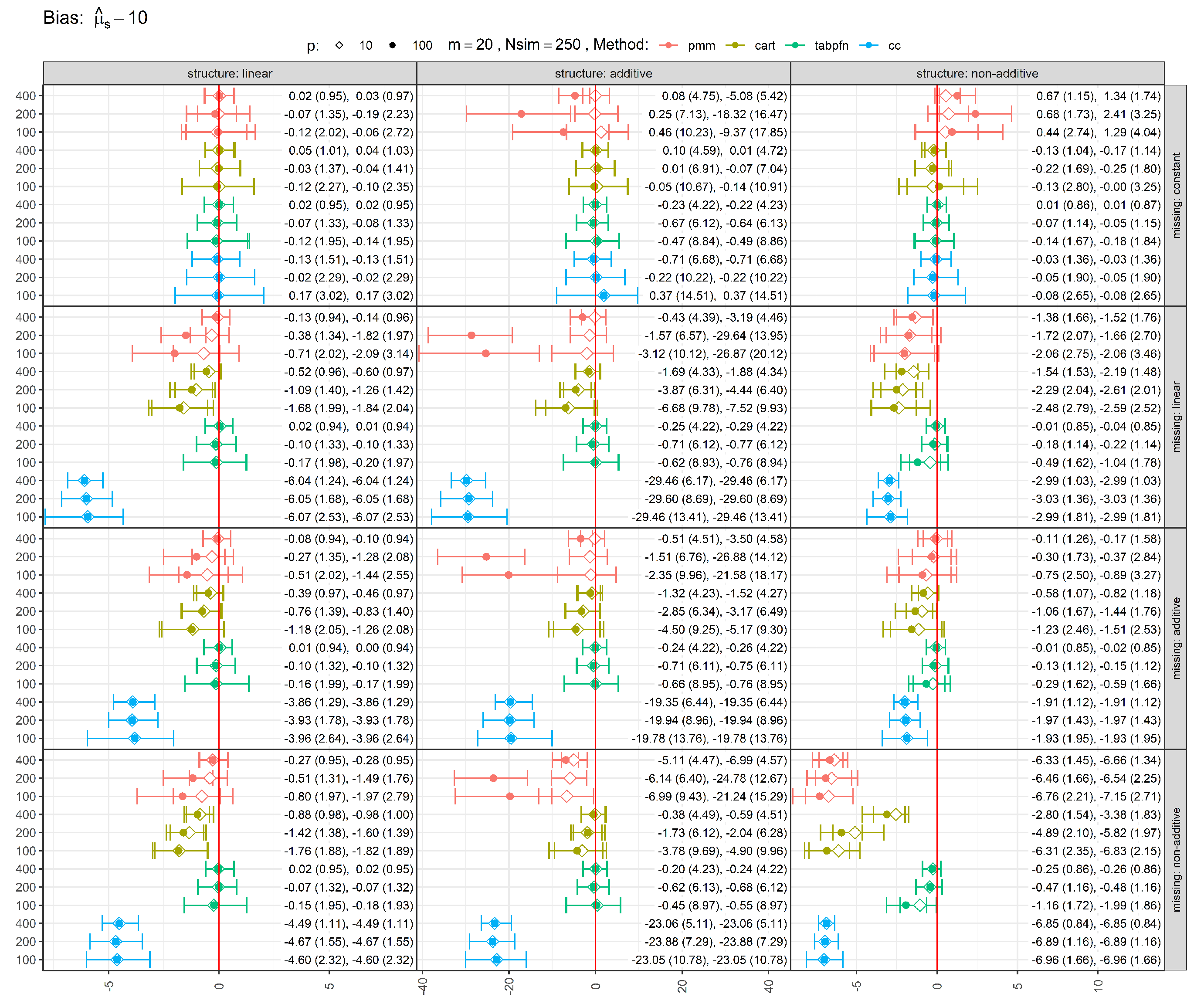
Figure 2.
Standard errors (SEs) of pooled estimates across imputation methods. Error bars indicate the 25th, 50th (median), and 75th percentiles; numbers report the mean and standard deviation in parentheses. The red vertical lines denote the median standard errors from the full-data analysis at the indicated sample size.
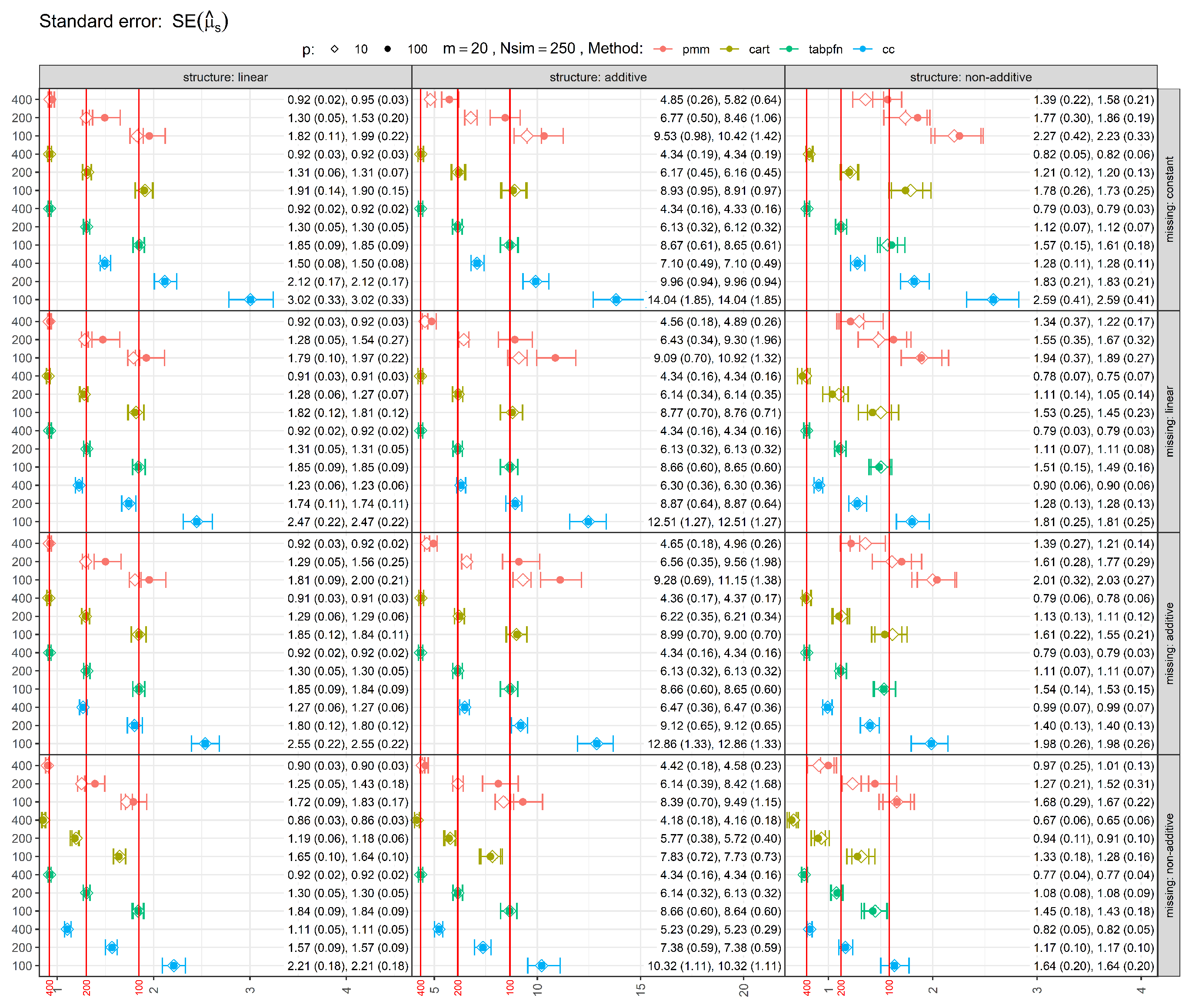
Figure 3.
Coverage rates of 90% Wilson confidence intervals across imputation methods. Ideally, coverage should be close to the nominal 95% level. The horizontal reference corresponds to nominal 95% coverage.
Figure 3.
Coverage rates of 90% Wilson confidence intervals across imputation methods. Ideally, coverage should be close to the nominal 95% level. The horizontal reference corresponds to nominal 95% coverage.
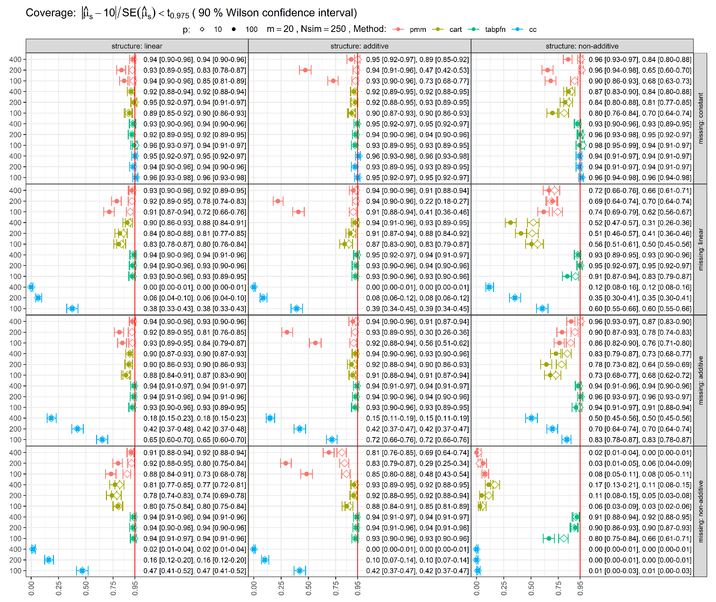
Table 1.
Average computational times (in seconds) required to generate imputations.
| Method | n | p=10 | p=100 |
|---|---|---|---|
| cart | 100 | 0.324 | 1.072 |
| cart | 200 | 0.373 | 1.281 |
| cart | 400 | 0.464 | 1.769 |
| pmm | 100 | 0.208 | 0.688 |
| pmm | 200 | 0.218 | 0.708 |
| pmm | 400 | 0.226 | 0.738 |
| tabpfn | 100 | 14.081 | 18.071 |
| tabpfn | 200 | 14.219 | 18.483 |
| tabpfn | 400 | 14.510 | 19.607 |
Table 2.
Comparison of g-computation and MI methods for estimating the ACE of smoking cessation on weight gain. MI imputes only the missing counterfactual outcomes, whereas g-computation replaces all outcomes with model predictions.
Table 2.
Comparison of g-computation and MI methods for estimating the ACE of smoking cessation on weight gain. MI imputes only the missing counterfactual outcomes, whereas g-computation replaces all outcomes with model predictions.
| Method | Estimate | Std.error | Lower 95% | Upper 95% |
|---|---|---|---|---|
| pmm | 2.363 | 0.834 | 0.728 | 3.998 |
| cart | 3.419 | 0.581 | 2.280 | 4.558 |
| tabpfn | 2.746 | 0.568 | 1.633 | 3.859 |
| g-computation | 3.380 | 0.853 | 1.708 | 5.053 |
Disclaimer/Publisher’s Note: The statements, opinions and data contained in all publications are solely those of the individual author(s) and contributor(s) and not of MDPI and/or the editor(s). MDPI and/or the editor(s) disclaim responsibility for any injury to people or property resulting from any ideas, methods, instructions or products referred to in the content. |
© 2026 by the author. Licensee MDPI, Basel, Switzerland. This article is an open access article distributed under the terms and conditions of the Creative Commons Attribution (CC BY) license.
Copyright: This open access article is published under a Creative Commons CC BY 4.0 license, which permit the free download, distribution, and reuse, provided that the author and preprint are cited in any reuse.


