Submitted:
14 June 2024
Posted:
17 June 2024
You are already at the latest version
Abstract
Multiple imputation by chained equations (MICE) is a popular and well-researched statistical approach to account for missing data in empirical research. However, applying the technique requires researchers to set dozens of smaller and larger parameters to build an adequate imputation model before estimating the analytical model of interest. It is somewhat unclear how severely small and potentially arbitrary decisions influence the quality of the produced findings. The current study tests this empirically using a simulation approach with datasets with low and high shares of missing data points that are missing at random (MAR). For each of the two specifications, 4,200 simulations are conducted where multiple parameters are randomly varied to create a diverse range of potential imputation models. The results demonstrate that even random imputation models can significantly reduce bias compared to listwise deletion since more than 90% of all simulations give less biased results. All minor decisions taken together explain between 11% and 21% of the variation in the statistics of interest. The most substantial influence on this variation is due to the selection of the imputation algorithm within MICE. These findings demonstrate that almost any imputation model, even those built with little care, will often result in a higher quality than applying listwise deletion, as long as critical assumptions, such as MAR and the avoidance of severe misspecifications, hold.
Keywords:
MICE
; missing data
; imputation
; item-nonresponse
; simulation study
; dominance analysis
1. Introduction
Missing data is a common problem in all areas of empirical research. Whenever some data points are missing, researchers are faced with the obstacle of incomplete information, which can introduce bias and lead to wrong statistical conclusions. While in the past, simply removing cases with incomplete data, also known as listwise deletion, was common due to the unavailability of adequate other solutions, the imputation of missing data has made much progress in the last decades. While early approaches, such as the imputation by mean values or with regression models, could introduce other sources of bias, such as an underestimation of the variation of the statistic of interest, methods such as multiple imputation by chained equations (MICE), a form of stochastic imputation, provide a much higher quality (Allison, 2002; Horton & Kleinman, 2007). For multiple reasons, MICE has become one of the de-facto standards in empirical research: the approach has been investigated in much detail from a statistical perspective and delivers satisfactory results under the right circumstances (Azur et al., 2011; van Buuren, 2018). The statistical approach is accessible and can be understood by most researchers even without a background in statistics. Finally, the algorithm has been implemented in most statistical packages, such as R, SPSS, Stata, or SAS, making it available to most researchers.
However, depending on the data and research question, imputation can be a significant challenge in the research process. After the analytic model has been selected (the main model the researcher wants to estimate to obtain the statistics of interest), the imputation model must be built. While the general rule of thumb is that the imputation model must, at least, include all variables of the analytic model, there are no limitations to how complex the imputation model can become. In this process, numerous - smaller and larger - decisions have to be made as even simple imputation models sometimes require setting dozens of parameters. While some rules are well established (such as the higher the number of generated imputations, the higher the precision), other questions are not well-researched, and trial-and-error is a common approach. While diagnostic methods are available to gauge some aspects of the quality of the generated data, when the number of parameters is large, it is often not feasible to test dozens or even hundreds of potential models, given the combinatorial diversity that quickly emerges. The main research question that arises from such standard practices is as follows: how strongly do (mostly) arbitrary decisions of the imputation model affect the quality of the analytic model? In the following, this question will be investigated using a relatively simple analytic model and statistical simulations to gauge the influence of dozens of parameters on the final outcome. Since in simulation studies, the “true” effect is known, the overall quality of the results can be estimated. It must be made clear that it is not the research goal of the current study to assess the overall quality of some approaches or algorithms or give final recommendations (“X is the best imputation algorithm”) given the virtually unlimited range of research questions and data constellations. Instead, it should be made transparent how apparently small decisions can influence research results and are a potential factor of (additional) bias and variance.
2. Imputing with MICE
In the following, the basic approach to conducting statistical analyses is outlined in the presence of missing data under the application of MICE, first proposed by Rubin (2004). Due to space constraints, the detailed algorithms are not explained, and references to the literature are made (Wulff & Jeppesen, 2017). However, various more minor decisions are outlined that a researcher faces when using the approach.
As a first step, the primary analytical model must be decided upon, which is a consequence of the research question. This usually requires deciding on a statistical model or approach (descriptive analysis, regression model, statistical matching, ...) and all variables that are required to carry out the analyses. We assume a simple regression model has been chosen in the following. This means the dependent variable and one or multiple independent variables are selected. We furthermore assume that imputation is feasible in general, meaning that the missingness is not too high, rendering the approach useless and that no monotonic missingness patterns are present. These potential problems can be tested empirically. The following gives an overview of parameters that need to be decided upon. Note that this is a partial list, as different variants of MICE or different software implementations might open up even more parameters to adjust. It can hence be a lower limit of potential complexity.
- Type of imputation distribution. One of the main advantages of MICE, in contrast to other approaches, is that a large variety of different distributions are available and that virtually all types of variables can be imputed. For example, continuous and normally distributed variables, such as body height or intelligence, can be imputed but also binary, ordinal, multinomial, or count variables. While some limitations are apparent (e.g., a multinomial variable should never be imputed using a linear model), other decisions are less clear. For example, a continuous and normally distributed variable can be imputed using a linear model and predictive mean matching (PMM). The advantage of PMM is that due to using donors from the data, only values are imputed that are already present in the data, and no impossible values can be generated (Landerman et al., 1997). However, PMM also requires the researcher to set another parameter, the number of potential donors to use (White et al., 2011). Furthermore, some variables have natural boundaries (such as height or income) which can never fall below zero. Some algorithms, such as truncated regression models, respect these limitations, while others do not.
- Adding auxiliary variables to the model. As described above, the imputation model must contain all variables of the analytic model. However, adding even more variables to the imputation model only can be beneficial to improve the quality. Usually, these are variables that have none or only very little missing information and are highly correlated with the other variables, making them good predictors (Schafer, 2003). These variables will not show up in the analytic models (since this potentially leads to high multicollinearity or undermines the effect of interest due to being mediators). However, they can increase the precision of the imputed values and decrease bias. The question arises of which auxiliary variables to use and how many. Large datasets can potentially contain many of these, and researchers can use other statistical approaches, such as correlation analyses, to select them. While the consensus is that auxiliary variables, in general, can be helpful, there are no strict guidelines. Also, survey weights can benefit the imputation model as they add further information to the statistical model (Kim et al., 2006).
- Adding interaction terms or higher order terms. As a rule of thumb, when the analytic model contains an interaction term or a higher order term (squares of cubes of variables), these should also be added to the imputation model (often as “just another variable”) (Seaman et al., 2012). However, when the analytic model does not contain them, they might still be helpful in the imputation model. Which interactions or how many to include is less clear.
- Delete missing ys or not. When the dependent variable also has missing values, it is clear that it still must be included in the imputation model. Some researchers argue, however, that these cases, where the dependent variable has been imputed, should be deleted afterward and not be used in the analytic model (von Hippel, 2007). Others argue that this step is unnecessary, especially when strong predictors of the dependent variable are available (Sullivan et al., 2015). While some simulation results are available, no clear consensus is reached.
- Bootstrapping or not. Bootstrapping can generated standard errors and derived statistics, such as confidence intervals, by sampling repeatedly from the available data with replacement and is an alternative to (parametric) approaches (Bittmann, 2021; Efron & Tibshirani, 1994). Posterior estimates of model parameters can be obtained using sampling with replacement, which is called bootstrapping. Otherwise, most algorithms use a large-sample normal approximation of the posterior distribution. While bootstrapping can be beneficial when asymptotic normality of parameter estimates is not given, it is mostly unclear how influential this decision is. Note that this specification must be distinct from the fact that one can combine bootstrapping and imputation methods to generate confidence intervals for a statistic that has no analytic standard errors (Brand et al., 2019).
- Number of imputations. In general, the higher the number of imputations produced under MICE, the better the quality, as the influence of random Monte-Carlo error is decreasing (von Hippel, 2020). While in the past, even five imputations were seen as sufficient, increased computational power has made the usage of dozens or even hundreds of imputations feasible. While more is better, selecting a final number of imputations is not written in stone and only rules of thumb are available.
Summarized, the combinatorial diversity of these more minor decisions can lead to hundreds or even thousands of potential imputation models, from which a final model has to be selected. In the following, a design will be proposed to test the influence of these decisions on actual imputation results. It is the goal of the following empirical analyses to gauge how influential these more minor decisions are on produced statistical results. There are two primary outcomes: the statistic of interest (a regression coefficient) and its standard error. By analyzing the bias and the variability of generated statistics, the quality of the imputation process can be assessed.
3. Empirical Analyses
3.1. Data
The data source for the following analyses is the National Longitudinal Survey of young women from 1968 to 1988. The dataset contains longitudinal information about the working situation of women, such as year of birth, place of residence, wages, or union membership. This serves as a suitable source. The data were reduced to the entries of 1988, and a random sample of 750 individuals with complete data was drawn. Six key variables were retained: hourly wages in dollars (wage), hours worked per week (hours), total labor force experience (ttl_exp), current age (age), work experience in the current job (tenure), and years of schooling completed (grade). The wages of 1982 were also retained in an extra variable (wage0). The data were amputed, that is, missingness in the complete data was created for the following analyses. The critical assumption is that missingness must be missing at random (MAR), meaning that missingness in a variable is partially correlated with observed variables. If the data were missing not at random (MNAR), imputation could not improve the data quality since missingness is due to unobserved influence. If the missingness were completely at random (MCAR), imputation would also not benefit the results, as listwise deletion would give unbiased estimates. The four variables of the following analytical model were specified to have missing values: wage, hours, ttl_exp, and age. The probability of missingness is generated using a logistic link function under the influence of all other variables in the model. Tenure, grade, and wage0 are auxiliary variables and have no missing values. Two conditions are specified: a rather low share of missingness per variable (14.97%) and a high share of missingness (29.07%). These shares were selected since they are realistic in empirical research yet are still tolerable so that imputation can improve results (Knol et al., 2010). No particular patterns were specified, meaning that the share of missingness of a variable does not depend on other variables. A descriptive overview of the three datasets is provided in Table 1. A correlation table that lists how strongly all variables in the model predict missingness is listed in the Appendix in Table A1.
3.2. Strategy of Analysis
The analytical model is defined as follows:
wage = α + β0 ttl_exp + β1 hours + β2 age
The goal is to estimate the effect of total labor force experience on hourly wages under the statistical control of hours worked per week and current age. β0 is, therefore, the coefficient of interest as it expresses how much an additional year of experience influences wages. The method of choice is a linear (OLS) regression model since all variables are continuous and linear effects are to be approximated. We can regard the results of the complete dataset as our benchmark. Regression results are reported in Table 2.
The model using the complete data reports a coefficient of 0.318, meaning that each additional year of work experience increases wages by about 32 cents under the control of age and hours worked per week. In the model with low missingness, the total number of cases available reduces to 428 due to listwise deletion, as even a single missing data point results in the loss of the entire case. The estimated coefficient is smaller and apparently biased. This becomes even more critical in the model with high missingness, where only 241 cases can be utilized. The resulting coefficient is highly biased. However, standard errors are quite similar in all three models.
In the following simulation, we impute data using MICE and estimate the analytical model. Of interest is the estimated regression coefficient of total labor force experience (ttl_exp) and its standard error. As described before, the following parameters are varied:
- Imputation algorithm (OLS regression, truncated regression (for variable wage only), predictive mean matching with 2, 6, 10, or 14 matches)
- Analytic or bootstrap standard errors in imputation models
- Adding higher-order terms and / or interaction terms
- Using up to three auxiliary variables
- Removing cases where the dependent variable has been imputed or not before the estimation of the analytic model
These different options are randomly selected, leading to a large number of potential imputation models (theoretically, all combinations of empirically available variables lead to a universe of more than 3.8 million imputation models). To minimize the influence of random Monte-Carlo error, a large number of imputations (75) is selected for each imputation model. This parameter is not varied in the imputations since it is well known that more imputations will lead to more precise results. The simulation is carried out separately for the two datasets with missing data. 4,200 simulations are conducted per dataset (if some imputations did not converge statistically, they were removed and the missing imputations were repeated with another random imputation model). All analyses are carried out using Stata 16.1, and the random specifications for the imputation model are selected using a script written in Python 3. Dominance analyses are computed using the Stata package domin (Luchman, 2015).
Of particular interest for the evaluation of the results are the following statistics: First, the overall variability in produced coefficients and standard errors. Second, whether a specific imputation actually improves the data quality and approximates, as best as possible, the unbiased result of the complete dataset. Third, the contribution of each imputation parameter to the result and decomposition of the overall explained variance. These analyses make it possible to understand in more detail how much these various decisions in the imputation stage can affect outcomes.
4. Results
The main results of the simulation study and the simulation specifications are summarized in Table 3. The upper part contains the generated statistics of interest, and the lower part the overview of the used imputation models.
Of particular interest is how well the imputations were able to approximate the unbiased effects, as reported in Table 2, with a regression coefficient for ttl_exp of 0.318 and a standard error of 0.0558. Interestingly, in both specifications, the coefficient is well approximated, and the bias of the listwise regressions is greatly attenuated. This nicely highlights why imputation can clearly benefit results. The average standard error of this regression coefficient is larger than the unbiased one. This makes sense as there is less information available, which imputation can only reduce to a certain degree. These results are also visualized in Figure 1.
The main finding is that 90% (low missingness) or even 94% (high missingness) of the imputation models have a regression coefficient that is closer to the unbiased one than the coefficient generated with listwise deletion. However, there is clearly also variation in the produced estimates. Another way to visualize the quality of the imputation results is by sorting the generated coefficients by value and plotting them with their respective 95% confidence intervals, which is done in Figure 2. As we see, the produced results are usually quite close to the unbiased regression coefficient (dotted horizontal lines), while some outliers at the tails are produced as well.
The lower part of the table lists the specifications of the imputation models (algorithm specifications not depicted due to space constraints). For binary choices, the average usage of 50% is well approximated.
Next, the absolute difference between the unbiased statistic and the imputed statistic is computed for the coefficient of interest and its standard error. Apparently, the smaller this difference, the better the imputation model. These are the dependent variables. All variables of the imputation models are the explanatory variables. Using linear (OLS) regressions, we can now estimate a.) the overall explained variance by the specifications in the imputation models and b.) the regression coefficients of all explanatory variables. Standardized (beta) coefficients are reported in Table 4.
As the results show, the imputation specifications explain between 11.3% and 21.1% of the overall variance, depending on the share of missingness and the statistic of interest (regression coefficient or standard error). Some variables exert a statistically highly significant influence, such as the inclusion of wage of a previous survey wave. As the specifications were generated randomly and independent of each other, the ceteris paribus interpretation holds. For this specific parameter, the conclusion is that the inclusion of wage of a previous wave reduces the error of the estimated regression coefficient of ttl_exp by 0.087 standard deviations (specification with low missingness). However, as explained before, these numbers should not be generalized uncritically, as the specific data constellations might be influential as well.
Finally, the explained variance of each model must be decomposed so the relative influence of each variable or decision can be gauged. To do so, dominance analysis is a popular approach (Azen & Budescu, 2003; Budescu, 1993). Whenever correlated explanatory variables are present, a simple nested regression approach is not adequate to isolate the effect of specific variables or groups of variables. Dominance analysis is a computationally intense approach, as through testing all possible combinations of predictors, the relative influence of each can be quantified, even if predictors are correlated. The sum of all parts is then the total explained variance by the complete model, which is reported in Table 4. For a more convenient interpretation, various independent variables are grouped together. The results with respect to R² are visualized in Figure 3.
Apparently, the choice of imputation algorithm explains the most variance of the outcome variable (absolute error difference for the coefficient of interest or its standard error). Also rather influential is whether or not to delete missing ys after the imputation. Interestingly, whether or not to include auxiliary variables has a comparably small influence.
5. Discussion and Conclusion
As the findings have demonstrated, imputing missing data with MICE can be highly beneficial to obtain less biased findings. Quite surprisingly, even in settings with a relatively large share of missing data, an imputation model where all minor decisions are randomized delivers satisfactory results and is in more than 90% of all simulations better than not imputing at all. While there is variation in the quality of the results, measured in the absolute error of the statistic of interest and its standard error, this is still better than using listwise deletion, where especially coefficients can be heavily biased. This is the crucial message to researchers: almost any imputation is better than no imputation. As the extended results have also shown, the choice of imputation algorithm is usually the most influential one, while others, such as the inclusion of interactions or bootstrapping in the imputation model, are of minor influence. Therefore, researchers should pay special attention to this aspect.
Nonetheless, the current findings come with some limitations. First, as research questions and data constellations can be virtually unlimited, a single simulation study can never answer posed research questions exhaustively. While the simulation attempted to be somehow realistic, other scenarios might be very different. The central assumption made was that imputation, in general, is feasible as MAR holds true. If other observed variables cannot predict missingness, imputation will not reduce bias and can even create more random variation in outcome statistics. Second, even in the random imputations, severe misspecifications did not occur due to the choice of eligible values for all varied parameters. Researchers still need to look at each variable in detail, theoretically and empirically. In the simulation, it was not possible to select an utterly wrong imputation model, such as imputing a nominal variable (think of the place of residence) using a linear model, which will create nonsensical results. The imputation algorithm must somehow fit the empirically observed distribution. As we have seen, even the choice between generally suitable algorithms does influence the results to some extent.
To summarize, these findings do not mean that researchers should build their imputation models without care and sloppily, as a sophisticated model can deliver even better and less biased results. Instead, researchers, also those with little experience using imputation techniques, should be encouraged to apply approaches such as MICE instead of listwise deletion, as more minor errors are probably forgiven as long as central model specifications are acceptable.
Funding
This research received no specific grant from any funding agency in the public, commercial, or not-for-profit sectors.
Data availability
Data are available from http://www.stata-press.com/data/r9/nlswork.dta (2022-11-28). Complete Do-files are available on request.
Conflict of interest
The author states that he has no conflict of interest.
Appendix A

Table A1.
Correlation between generated missing values and other variables in the datasets.
| Missing wage | Missing age | Missing hours | Missing ttl_exp | |
| Low missingness | ||||
| Hours per week | 0.200*** | 0.178*** | 0.126*** | |
| Age | 0.0877* | 0.0249 | 0.112** | |
| Total work experience | 0.177*** | 0.183*** | 0.178*** | |
| Completed school years* | 0.166*** | 0.220*** | 0.109** | 0.165*** |
| Current work experience* | 0.168*** | 0.191*** | 0.147*** | 0.142*** |
| Wage (t-1)* | 0.171*** | 0.200*** | 0.177*** | 0.233*** |
| Wage | 0.200*** | 0.265*** | 0.181*** | |
| High missingness | ||||
| Hours per week | 0.243*** | 0.205*** | 0.229*** | |
| Age | 0.0481 | -0.00207 | 0.101** | |
| Total work experience | 0.227*** | 0.208*** | 0.195*** | |
| Completed school years | 0.170*** | 0.164*** | 0.221*** | 0.196*** |
| Current work experience | 0.234*** | 0.251*** | 0.215*** | 0.223*** |
| Wage (t-1) | 0.259*** | 0.217*** | 0.263*** | 0.163*** |
| Wage | 0.248*** | 0.298*** | 0.199*** | |
| Observations | 750 | 750 | 750 | 750 |
Source: NLSWork88. Auxiliary variables marked with an asterisk. Reported are Pearson’s R correlation coefficients. * p < 0.05, ** p < 0.01, *** p < 0.001.
References
- Allison, P. (2002). Missing Data. Thousand Oaks, CA: Sage.
- Azen, R., & Budescu, D. V. (2003). The dominance analysis approach for comparing predictors in multiple regression. Psychological Methods, 8(2), 129–148. [CrossRef]
- Azur, M. J., Stuart, E. A., Frangakis, C., & Leaf, P. J. (2011). Multiple imputation by chained equations: What is it and how does it work?: Multiple imputation by chained equations. International Journal of Methods in Psychiatric Research, 20(1), 40–49. [CrossRef]
- Bittmann, F. (2021). Bootstrapping: An Integrated Approach with Python and Stata (1st ed.). De Gruyter. [CrossRef]
- Brand, J., Buuren, S., Cessie, S., & Hout, W. (2019). Combining multiple imputation and bootstrap in the analysis of cost-effectiveness trial data. Statistics in Medicine, 38(2), 210–220. [CrossRef]
- Budescu, D. V. (1993). Dominance analysis: A new approach to the problem of relative importance of predictors in multiple regression. Psychological Bulletin, 114(3), 542–551. [CrossRef]
- Efron, B., & Tibshirani, R. J. (1994). An introduction to the bootstrap. CRC press.
- Horton, N. J., & Kleinman, K. P. (2007). Much Ado About Nothing: A Comparison of Missing Data Methods and Software to Fit Incomplete Data Regression Models. The American Statistician, 61(1), 79–90. [CrossRef]
- Kim, J. K., Michael Brick, J., Fuller, W. A., & Kalton, G. (2006). On the bias of the multiple-imputation variance estimator in survey sampling. Journal of the Royal Statistical Society: Series B (Statistical Methodology), 68(3), 509–521. [CrossRef]
- Knol, M. J., Janssen, K. J. M., Donders, A. R. T., Egberts, A. C. G., Heerdink, E. R., Grobbee, D. E., Moons, K. G. M., & Geerlings, M. I. (2010). Unpredictable bias when using the missing indicator method or complete case analysis for missing confounder values: An empirical example. Journal of Clinical Epidemiology, 63(7), 728–736. [CrossRef]
- Landerman, L. R., Land, K. C., & Pieper, C. F. (1997). An Empirical Evaluation of the Predictive Mean Matching Method for Imputing Missing Values. Sociological Methods & Research, 26(1), 3–33. [CrossRef]
- Luchman, J. N. (2015). “DOMIN”: Module to conduct dominance analysis. Boston College Department of Economics. https://ideas.repec.org/c/boc/bocode/s457629.html.
- Rubin, D. B. (2004). Multiple imputation for nonresponse in surveys (Vol. 81). John Wiley & Sons.
- Schafer, J. L. (2003). Multiple Imputation in Multivariate Problems When the Imputation and Analysis Models Differ. Statistica Neerlandica, 57(1), 19–35. [CrossRef]
- Seaman, S. R., Bartlett, J. W., & White, I. R. (2012). Multiple imputation of missing covariates with non-linear effects and interactions: An evaluation of statistical methods. BMC Medical Research Methodology, 12(1), 46. [CrossRef]
- Sullivan, T. R., Salter, A. B., Ryan, P., & Lee, K. J. (2015). Bias and Precision of the “Multiple Imputation, Then Deletion” Method for Dealing With Missing Outcome Data. American Journal of Epidemiology, 182(6), 528–534. [CrossRef]
- van Buuren, S. (2018). Flexible imputation of missing data (Second edition). CRC Press, Taylor and Francis Group.
- von Hippel, P. T. (2007). 4. Regression with Missing Ys: An Improved Strategy for Analyzing Multiply Imputed Data. Sociological Methodology, 37(1), 83–117. [CrossRef]
- von Hippel, P. T. (2020). How Many Imputations Do You Need? A Two-stage Calculation Using a Quadratic Rule. Sociological Methods & Research, 49(3), 699–718. [CrossRef]
- White, I. R., Royston, P., & Wood, A. M. (2011). Multiple imputation using chained equations: Issues and guidance for practice. Statistics in Medicine, 30(4), 377–399. [CrossRef]
- Wulff, J. N., & Jeppesen, L. E. (2017). Multiple imputation by chained equations in praxis: Guidelines and review. Electronic Journal of Business Research Methods, 15(1), 41–56.
Figure 1.
Histograms of generated coefficients and standard errors by missingness specification.
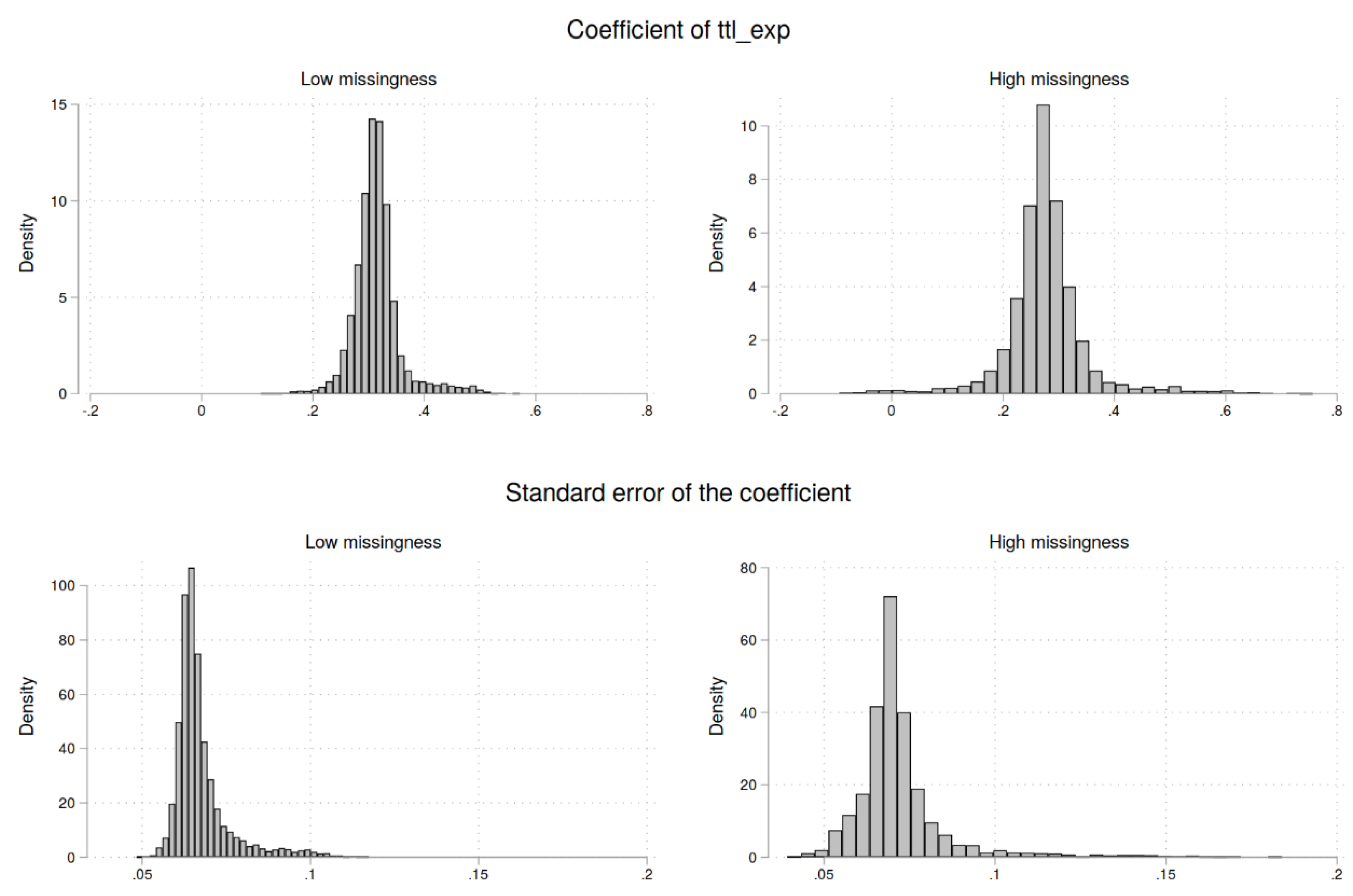
Figure 2.
Generated coefficients and confidence intervals by missingness specification. Note: the dashed horizontal line marks the unbiased regression coefficient.
Figure 2.
Generated coefficients and confidence intervals by missingness specification. Note: the dashed horizontal line marks the unbiased regression coefficient.
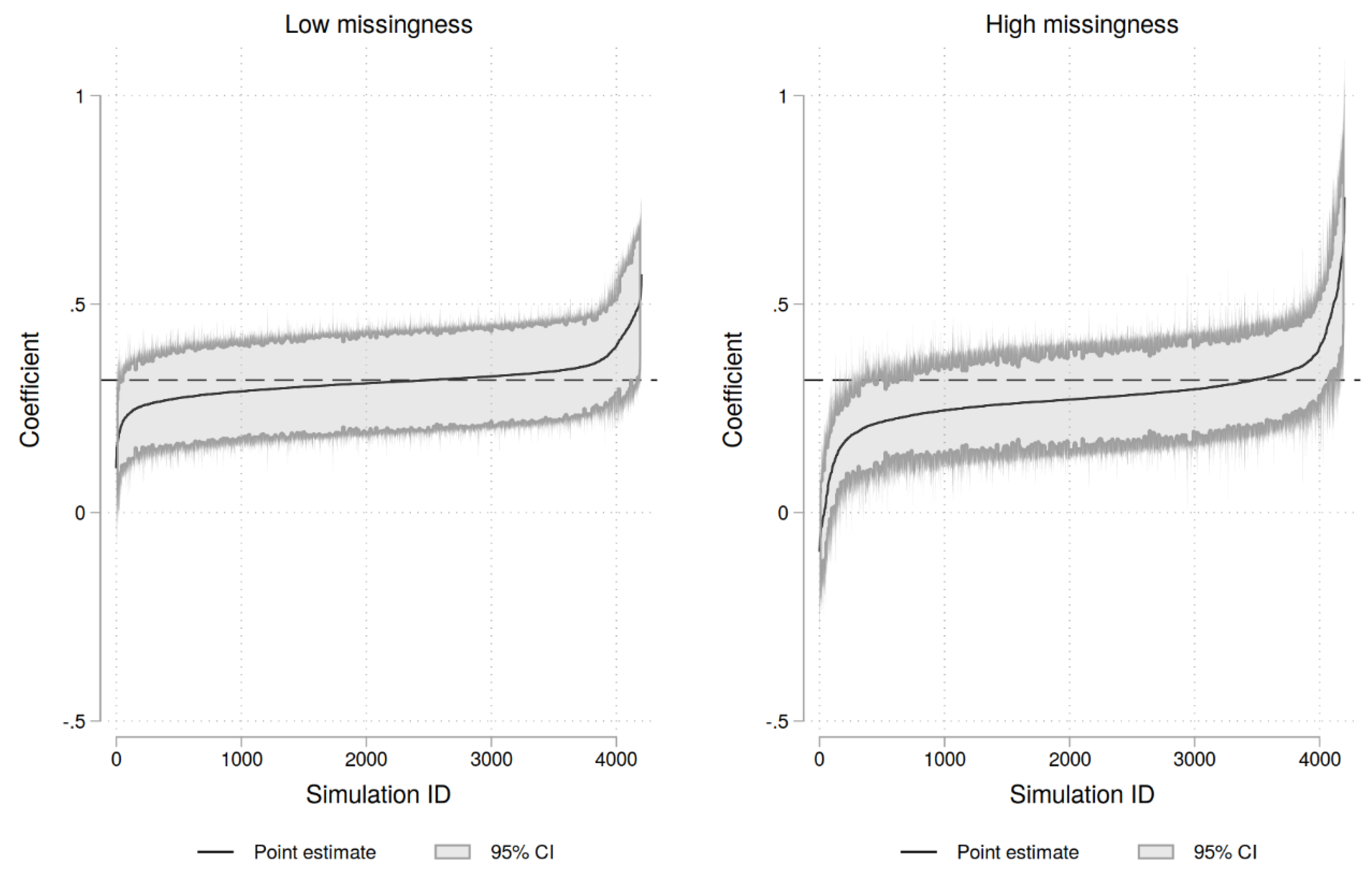
Figure 3.
Variance decomposition by statistic of interest (absolute difference to unbiased statistic) and missingness specification.
Figure 3.
Variance decomposition by statistic of interest (absolute difference to unbiased statistic) and missingness specification.
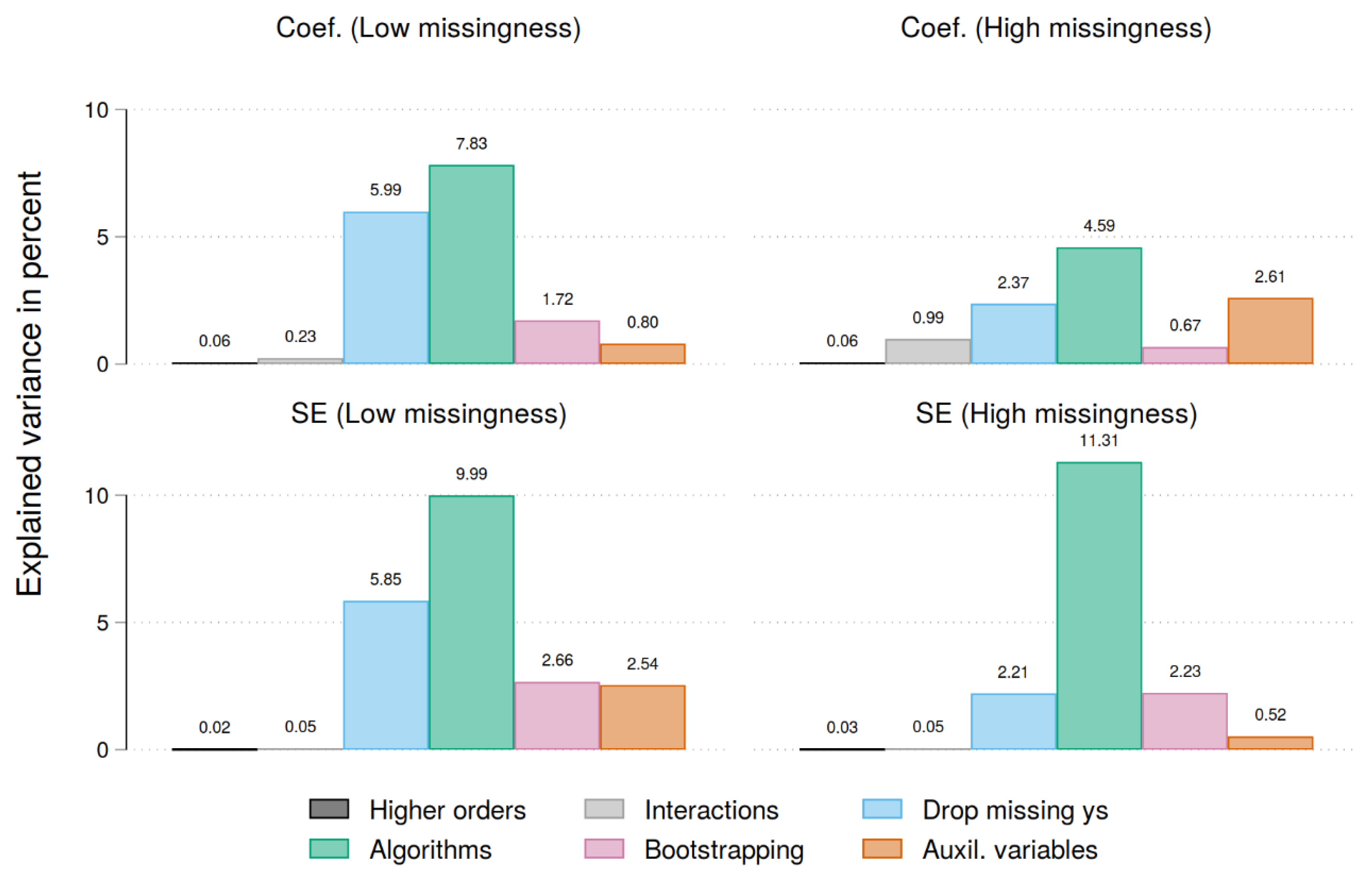
Table 1.
Descriptive overview by missingness specification.
| Complete data | Low missingness | High missingness | |||||||
| N | Mean | SD | N | Mean | SD | N | Mean | SD | |
| Wage | 750 | 8.07 | 5.98 | 644 | 7.80 | 5.89 | 534 | 7.24 | 5.38 |
| Total work experience | 750 | 13.7 | 3.92 | 624 | 13.5 | 3.97 | 484 | 13.3 | 3.99 |
| Hours per week | 750 | 37.8 | 9.72 | 656 | 37.7 | 9.92 | 565 | 37.5 | 9.84 |
| Age | 750 | 39.2 | 3.11 | 627 | 39.1 | 3.14 | 545 | 39.1 | 3.09 |
| Wage (t-1)* | 750 | 6.34 | 3.14 | 750 | 6.34 | 3.14 | 750 | 6.34 | 3.14 |
| Current work experience* | 750 | 6.84 | 5.70 | 750 | 6.84 | 5.70 | 750 | 6.84 | 5.70 |
| Completed school years* | 750 | 12.9 | 2.41 | 750 | 12.9 | 2.41 | 750 | 12.9 | 2.41 |
Source: NLSWork88. N gives the number of cases with complete information. Auxiliary variables are marked with an asterisk and are never missing.
Table 2.
OLS regression results for complete and missing data.
| Complete data | Low missingness | High missingness | |
| Total work experience | 0.318*** | 0.251*** | 0.143* |
| (0.0558) | (0.0506) | (0.0556) | |
| Hours per week | 0.0467* | 0.0449* | 0.0288 |
| (0.0223) | (0.0203) | (0.0224) | |
| Age | -0.106 | -0.201** | 0.0570 |
| (0.0695) | (0.0650) | (0.0696) | |
| Constant | 6.106* | 9.571*** | 0.666 |
| (2.861) | (2.704) | (2.944) | |
| Observations | 750 | 428 | 241 |
| R2 | 0.054 | 0.092 | 0.037 |
Source: NLSWork88. Unstandardized regression coefficients. Standard errors in parentheses. * p < 0.05, ** p < 0.01, *** p < 0.001.
Table 3.
Simulation results by missingness specification.
| Low missingness | High missingness | |||||||
| mean | sd | p5 | p95 | mean | sd | p5 | p95 | |
| Coef. ttl_exp | 0.31 | 0.044 | 0.26 | 0.39 | 0.28 | 0.078 | 0.17 | 0.39 |
| SE of ttl_exp | 0.067 | 0.0085 | 0.060 | 0.086 | 0.072 | 0.015 | 0.056 | 0.099 |
| Better than listwise deletion | 0.90 | 0.30 | 0 | 1 | 0.94 | 0.23 | 0 | 1 |
| Bootstrap wage | 0.51 | 0.50 | 0 | 1 | 0.50 | 0.50 | 0 | 1 |
| Bootstrap hours | 0.49 | 0.50 | 0 | 1 | 0.49 | 0.50 | 0 | 1 |
| Bootstrap age | 0.50 | 0.50 | 0 | 1 | 0.51 | 0.50 | 0 | 1 |
| Bootstrap ttl_exp | 0.50 | 0.50 | 0 | 1 | 0.49 | 0.50 | 0 | 1 |
| Auxil. tenure | 0.50 | 0.50 | 0 | 1 | 0.50 | 0.50 | 0 | 1 |
| Auxil. education | 0.52 | 0.50 | 0 | 1 | 0.52 | 0.50 | 0 | 1 |
| Auxil. wage (t-1) | 0.52 | 0.50 | 0 | 1 | 0.52 | 0.50 | 0 | 1 |
| Number of higher-order terms | 1.43 | 0.85 | 0 | 3 | 1.42 | 0.84 | 0 | 3 |
| Number of interactions | 1.58 | 0.95 | 0 | 3 | 1.60 | 0.93 | 0 | 3 |
| Drop missing ys before estimation | 0.49 | 0.50 | 0 | 1 | 0.52 | 0.50 | 0 | 1 |
| Observations | 4200 | 4200 | ||||||
Note: detail specifications of the algorithms for all variables are not included due to space constraints. P5 = percentile 5; p95 = percentile 95.
Table 4.
OLS regression results to test the influence of imputation specifications on generated statistics by missingness specification.
Table 4.
OLS regression results to test the influence of imputation specifications on generated statistics by missingness specification.
| Low missingness | High missingness | |||||||
| Abs. diff. to unbiased coef. | Abs. diff. to unbiased SE | Abs. diff. to unbiased coef. | Abs. diff. to unbiased SE | |||||
| Bootstrap wage | 0.132*** | (0.001) | 0.163*** | (0.000) | 0.079*** | (0.002) | 0.149*** | (0.000) |
| Bootstrap hours | -0.005 | (0.001) | 0.013 | (0.000) | -0.025 | (0.002) | -0.015 | (0.000) |
| Bootstrap age | -0.002 | (0.001) | 0.011 | (0.000) | 0.002 | (0.002) | -0.021 | (0.000) |
| Bootstrap experience | -0.004 | (0.001) | 0.021 | (0.000) | -0.005 | (0.002) | 0.020 | (0.000) |
| Auxil. tenure | -0.021 | (0.001) | -0.108*** | (0.000) | 0.069*** | (0.002) | -0.035* | (0.000) |
| Auxil. education | -0.001 | (0.001) | 0.009 | (0.000) | -0.017 | (0.002) | -0.010 | (0.000) |
| Auxil. wage (t-1) | -0.087*** | (0.001) | -0.099*** | (0.000) | -0.175*** | (0.002) | -0.060*** | (0.000) |
| Number of higher order terms | 0.037* | (0.001) | -0.005 | (0.000) | 0.031 | (0.001) | 0.007 | (0.000) |
| Number of interactions | 0.053*** | (0.001) | 0.013 | (0.000) | 0.107*** | (0.001) | 0.013 | (0.000) |
| Drop missing ys | -0.247*** | (0.001) | -0.242*** | (0.000) | -0.160*** | (0.002) | -0.154*** | (0.000) |
| Algorithm (wage) | ||||||||
| OLS reg. | Ref. | Ref. | Ref. | Ref. | ||||
| PMM (2) | -0.000 | (0.002) | 0.003 | (0.000) | 0.008 | (0.003) | 0.033* | (0.001) |
| PMM (6) | -0.005 | (0.002) | -0.002 | (0.000) | -0.015 | (0.003) | -0.016 | (0.001) |
| PMM (10) | 0.005 | (0.002) | -0.015 | (0.000) | 0.008 | (0.003) | -0.029 | (0.001) |
| PMM (14) | -0.016 | (0.002) | -0.051*** | (0.000) | 0.007 | (0.003) | -0.074*** | (0.001) |
| Algorithm (hours) | ||||||||
| OLS reg. | Ref. | Ref. | Ref. | Ref. | ||||
| Trunc. reg. | 0.270*** | (0.001) | 0.296*** | (0.000) | 0.176*** | (0.002) | 0.308*** | (0.001) |
| PMM (2) | -0.036* | (0.002) | -0.015 | (0.000) | -0.006 | (0.003) | 0.023 | (0.001) |
| PMM (6) | -0.024 | (0.001) | -0.015 | (0.000) | 0.000 | (0.003) | 0.000 | (0.001) |
| PMM (10) | -0.003 | (0.001) | -0.012 | (0.000) | -0.009 | (0.003) | 0.024 | (0.001) |
| PMM (14) | 0.003 | (0.001) | 0.011 | (0.000) | -0.022 | (0.003) | 0.009 | (0.001) |
| Algorithm (ttl_exp) | ||||||||
| OLS reg. | Ref. | Ref. | Ref. | Ref. | ||||
| PMM (2) | -0.026 | (0.002) | -0.029* | (0.000) | -0.074*** | (0.003) | -0.026 | (0.001) |
| PMM (6) | -0.018 | (0.002) | -0.017 | (0.000) | -0.108*** | (0.003) | -0.062*** | (0.001) |
| PMM (10) | -0.032* | (0.001) | -0.041** | (0.000) | -0.064*** | (0.003) | -0.041** | (0.001) |
| PMM (14) | -0.034* | (0.001) | -0.031* | (0.000) | -0.085*** | (0.003) | -0.035* | (0.001) |
| Algorithm (age) | ||||||||
| OLS reg. | Ref. | Ref. | Ref. | Ref. | ||||
| PMM (2) | -0.011 | (0.001) | -0.027 | (0.000) | -0.010 | (0.003) | -0.005 | (0.001) |
| PMM (6) | 0.015 | (0.001) | 0.015 | (0.000) | -0.013 | (0.003) | -0.004 | (0.001) |
| PMM (10) | 0.013 | (0.001) | 0.026 | (0.000) | 0.016 | (0.003) | 0.021 | (0.001) |
| PMM (14) | 0.035* | (0.002) | 0.011 | (0.000) | -0.011 | (0.003) | 0.003 | (0.001) |
| Observations | 4200 | 4200 | 4200 | 4200 | ||||
| R2 | 0.166 | 0.211 | 0.113 | 0.164 | ||||
| Adjusted R2 | 0.161 | 0.206 | 0.107 | 0.158 | ||||
Standardized beta coefficients, standard errors in parentheses. PMM = Predictive Mean Matching. * p < 0.05, ** p < 0.01, *** p < 0.001.
Disclaimer/Publisher’s Note: The statements, opinions and data contained in all publications are solely those of the individual author(s) and contributor(s) and not of MDPI and/or the editor(s). MDPI and/or the editor(s) disclaim responsibility for any injury to people or property resulting from any ideas, methods, instructions or products referred to in the content. |
© 2024 by the authors. Licensee MDPI, Basel, Switzerland. This article is an open access article distributed under the terms and conditions of the Creative Commons Attribution (CC BY) license (http://creativecommons.org/licenses/by/4.0/).
Copyright: This open access article is published under a Creative Commons CC BY 4.0 license, which permit the free download, distribution, and reuse, provided that the author and preprint are cited in any reuse.


