Submitted:
23 February 2026
Posted:
25 February 2026
You are already at the latest version
Abstract
Despite the development of the new, modern non-metallic materials, the steel materials are largely used in various branches of industry, while in some applications they are still irreplaceable. It is expected that such a trend will remain for certain number of years. This is why the necessity is present for development of the new types of steels, which would possess even better properties. The Chromium-Molybdenum (Cr-Mo) steels, with high vanadium content, belong to the group of newer steels characterized by high values of hardness and toughness. In this research, the tests were performed on samples made from the X180CrMo12-1 steel with varying percentage of vanadium within the limits of 0.5-3%. Vanadium, as a carbide-forming alloying element, creates a carbide network of the M7C3 type around the metal matrix, and finely dispersed carbides of the V6C5 type within the metal matrix. This research was focused on determining the carbides’ composition, observing the shape of metal grains and carbide network, testing the material’s resistance to friction and wear, including the electrochemical characterization, as well. The objective was to determine the carbides microstructure and morphology, as well as to evaluate their impact on the material's characteristics. The experimental investigation was performed using the scanning electron microscopy with energy dispersive spectrometry (SEM-EDS) and X-ray diffractometric analysis (XRD). Examination of the carbide composition confirmed that it was the M7C3 carbide.
Keywords:
Cr-Mo steel
; vanadium
; carbides
; microstructure
; mechanical properties
; electrochemical analysis
1. Introduction
To obtain steels with optimal mechanical properties, certain alloying elements are added to their composition. Some of those elements create compounds - carbides during crystallization, both at the metal grains boundaries, as well as in the metal matrix [1]. The aim of this research was to determine the chemical composition of the carbides formed due to addition of vanadium to the tested steel. The chemical composition of the steel used in this research is given in Table 1.
The steel of this composition belongs to the group of quenchable steels [2]. The experiments were set to establish the impact of varying percentage of added vanadium and its carbides on changes in the microstructure of the examined material, and on its resistance to friction and wear. The electrochemical characterization of the tested material was conducted in three types of environments: acidic, neutral and alkaline [3,4,5].
Wen et al. (2013) [6] were studying influence of the vanadium content on carbides evolution in Fe–Cr–Ni–Mo high-strength steels by means of three-dimensional atom probe (3DAP) and transmission electron microscopy (TEM). The M2C and M6C carbides resulted due to addition of 0.03% or 0.08% V to steels, while M23C6 mainly appear when there is no V in the steel. The size of carbides generally decreased with increasing V content.
Chen, Chiu and West (2025) [7] have analyzed the influence of vanadium content on the microstructure evolution and mechanical behavior of CoCrFeNiVₓ high-entropy alloys (HEAs) synthesized via mechanical alloying (MA) and subsequent sintering. At the lower V level of 0.25 mol %, a single-phase FCC matrix with uniformly dispersed vanadium oxides was formed, with refined microstructure and a favorable combination of strength and ductility. On the other hand, at the higher V content of 0.75 mol %, microstructural transformations resulted in formation of a brittle Cr-rich σ phase and coarse vanadium oxides, which decreased ductility and led to embrittlement, despite an overall increase in hardness.
Sun, Wei and Lu (2020) [8] have dealt with influence of vanadium content on the precipitation evolution and mechanical properties of high-strength Fe–Cr–Ni–Mo weld metal. Authors concluded that the microstructures of the Fe–Cr–Ni–Mo weld metals with different V contents (0–0.18 wt %) did not exhibit major differences, but the V addition significantly increased the strength owing to the higher dislocation density and higher density of the discrete nanoscale MC carbides randomly distributed in the bainite.
Liu et al. (2024) [9] investigated the decomposition of the eutectic carbides at elevated temperatures of ductile casting steel (containing Ni, Cr, W, Mo, and V), produced by authors. The (Fe, Cr)-rich eutectic M3C carbides were completely decomposed after solutionized at 1050 ℃ for 7 h; the eutectic M6C carbides partially decomposed, with the morphology changes and the polygonal primary (V, W)-rich MC carbides underwent minimal changes even after solutionization at 1050 °C for 10 h, primarily due to their high thermal stability.
Gu et al. (2025) [10] were dealing with the effect of nitrogen substituting carbon on the high-temperature mechanical properties and wear performance of Cr–Mo–V hot-working die steel (HWDS). The substitution of nitrogen for carbon had a minimal impact on the wear mechanisms of the tested steel, while the substituting carbon improves the wear resistance at 500 °C, while reducing it at 600 °C. The difference in this effect is attributed to the varying roles played by undissolved V-rich carbides at different temperatures.
Huang et al. (2022) [11] reported the fluctuation of 4Cr5Mo2V steel properties with different contents of vanadium. The TEM results have indicated that the amount of MC-type stable precipitations increased with V content, while both the thermal stability and thermal conductivity declined. The higher content of V in experimental steels did not only postpone the secondary hardening, but exacerbated the coarsening of carbides and reduced the hardness, as well. Though this indicates that the coarsening and segregation of carbides have a detrimental effect on plasticity, the tensile and yield strengths at elevated temperature decreased constantly with V content.
Ren et al. (2024) [12] were considering the effect of tempering temperature on stress corrosion resistance of a low alloy high strength steel with high vanadium content. For the steel containing V (the T steel), with the increase of tempering temperature, the ferrite grain has coarsened, the size of vanadium carbide (VC) increased, while the number of VC decreased. The tensile strength decreased and the elongation increased, when tested in air. Compared to the steel without vanadium (the NT steel), the corrosion resistance of the T steel with vanadium was lowered. Additionally, simultaneously with the increase of tempering temperature, the effect brought by vanadium became more prominent.
Bialobrzeska (2024) [13] presented results on investigating the characteristics of the cast steel modified with chromium and vanadium, subjected to heat treatment. Author concluded that vanadium has positive effect on the strength parameters of this cast steel. The heat treatment had the positive effect on the fracture behavior of the tested steel, which became the mixed-type structure of a quasi- cleavage fracture.
Liu et al. (2019) [14] have studied the effect of vanadium micro-alloying on the microstructure evolution and mechanical properties of 718H pre-hardened mold steel. Authors assigned the strength increase to influence of the V addition on dislocation density, misorientation gradient, and fine scale MC precipitates. The yield strength of the tested steel was increased with increasing V content, while the transverse impact energy was decreased and similar behavior was exhibited by the longitudinal impact energy values.
Botero et al. (2021) [15] were dealing with Cr-Mo-V cold-work tool steel produced by electron beam melting (EBM), namely its microstructure and mechanical properties evaluation, prior to and after the adjusted heat treatment procedures. The microstructure was optimized by elimination of the Mo-rich carbides and by precipitation of V-rich carbides of various sizes. The properties of this steel were compared to those of a steel of the same composition produced by hot isostatic pressing. The former steel had superior properties as compared to the latter one. The only exception was ductility that exhibited the low values, which was ascribed to internal defects in the material.
Chen et al. (2023) [16] were considering the microstructure and mechanical properties of microwave-assisted sintered H13 steel powder. The tested material had varying proportions of vanadium powder, from 1.5 to 5.5. mass %. This is the first-time preparation of the block specimens by the microwave sintering. Results of the test have shown that the best wear behavior was exhibited by the material containing the 1.5% of vanadium powder.
2. Experimental Investigations
Samples for metallographic tests were prepared by the CO2 casting method in sand molds, in a medium-frequency induction furnace ASEA Brown Boveri – ABB, type ITMK-500 [17]. The samples sizes were 10×10×10 mm.
Four series of samples were made, and the composition of vanadium was varied: in the first series (I) 0.5%, in the second (II) 1%, in the third (III) 2% and in the fourth (IV) 3%. The chemical composition of samples for each batch is shown in Table 1.
After the casting, the samples were heat treated through the improvement process (quenching and tempering) at a temperature of 250 °C. After the heat treatment, slight deviations were noticed of the samples’ geometric forms and sizes. Due to that fact, the mechanical processing on a flat grinder had to be applied, with lubricating and cooling media, at room temperature. By grinding, with constant heat removal, all the unevenness and impurities were removed. The removal of the defective layer was carried out with a minimum cutting depth in several passes, up to the desired dimensions of 10×10 mm. Considering the small processing tolerances, the total grinding depth was less than 0.5 mm. In this way, no possible change of structure on the piece surface would have occurred.
Electron microscopy (SEM-EDS) was used to determine the chemical composition and microstructure. A JEOL brand scanning electron microscope, type JSM-6610LV, was used. By scanning microscopy, with the help of an EDS device, the chemical composition was determined of the phases present on the surface of the observed sample. In addition, a distribution map of influential chemical elements was created to understand and detect all the phases present in the examined sample.
Further tests were carried by the X-ray diffractometric analysis, to identify and calculate the lattice parameters. The analysis was performed on a Bruker D8 ADVANCE device, which is equipped with a dynamic scintillation detector and a ceramic X-ray Cu tube (KFL-Cu-2K) with a recording angle in the range of 10 to 150°. The samples for this analysis were ground and converted into a fine powder. Operating parameters were: step 0.02 ° 2θ and step time 20 s. This detection was carried out in the software package Topas 4.2 with the application of data from the ICCD database.
For tribological tests, to obtain the resistance to friction and wear of the investigated material, the CSM Nanotribometer of the "Ball-on-plate" type with the reciprocating movement, was used. The ball material was hard metal; the ball diameter was 1.5 mm. The tests were conducted under the following conditions: normal load 1 N, sliding speed 10 mm/s, amplitude 0.5 mm, number of cycles 5000/10 m, without lubrication. Friction and wear tests were performed on four samples’ series containing different percentages of vanadium (0.5, 1.0, 2.0 and 3.0 %). The measurements of each sample were repeated 5 times. In addition, corresponding photos of wear traces on the tested material and on the ball are provided. Computer-supported optical microscopes, manufactured by "MEIJI Techno", each of them was equipped with its own illuminator and high-resolution camera, were used for the analysis of the surfaces of the prepared samples, as well as of the resulting wear traces. Although the unlubricated friction in industrial conditions leads to greater wear of the parts [18], in this research it was chosen as the testing method due to the realistic conditions under which such steels are operating.
The hardness test was performed according to the standard procedure using the Vickers method. Microhardness was determined using a Digital microhardness tester, type DHV-1000. The applied load force was 0.245 N, and the pressing time was 20 s.
3. Results and Discussion
A clearly defined carbides’ network was observed around the martensite grains, and a small part of the carbides was finely dispersed in the metal matrix (Figure 1). The basic type of carbide was M7C3; its composition was determined by the EDS analysis.
The presence of vanadium, even at low contents, has a positive effect on highly alloyed Cr-Mo steels, because in the process of solidification, the V6C5 carbide crystals are formed from the melt, blocking the further growth of primary austenite dendrites, thus enabling the creation of a fine-grained structure [19,20,21]. Vanadium, as a distinctly carbide-forming element, not only forms grains of V6C5 carbide, but affects the morphology of M7C3 carbide, as well. It also reduces the stability of the austenite and generally refines the structure of the metal matrix. Similarly to iron, vanadium replaces chromium in the lattice of M7C3 carbide, which leads to an increase in the chromium content in the metal matrix and to a higher degree of hardenability of austenite.
3.1. Microstructural Analysis
The microstructure of a sample I, containing 1.8% C and 0.5% V is shown in Figure 1, where one can see the martensite crystals and a carbide network around the grains of the metal matrix, formed by the eutectic carbide M7C3. It has precipitated in the form of lamellae, plates and rosettes. The M7C3 carbide, in the two-dimensional space appears in the form of strips. A large number of those strips are usually grouped into bundles, having the same spatial orientation, thus in the two-dimensional space those bundles of strips appear resembling the lamellae. In Figure 1, the points where the EDS analysis was performed are marked from 1 to 5. For each of those points the measurements were repeated three times, and Table 3 provides the mean value of those three measurements. Maximum experimental deviations were ± 2.0%.
Chemical analysis was carried out for points 1, 2 and 5 of the metal matrix, and for points 3 and 4 of the carbide network. The analysis of the metal matrix indicates that it is dominated by martensite and residual austenite, but the increased contents of carbon and vanadium indicate the presence of finely dispersed vanadium carbides in the metal matrix.
Figure 2 shows the microstructure of sample number II with 1.8% C and 1% V. The chemical analysis of the metal matrix was performed at point 1, and at points 2, 3 and 4, a carbide analysis was performed. Table 3 shows the chemical composition of the tested phases of sample I, and Table 4 shows the chemical analysis of the examined phases of sample II.
Figure 3 shows the microstructure of sample number III and Figure 4 of sample number IV, with 1.8% C and 2% V, respectively. For sample number III, points 2, 3 and 4 in the figure indicate the places where the chemical analysis of the carbide was performed, and point 1 shows the place where the chemical analysis of the metal matrix was performed. Chemical composition of the tested phases of sample III is presented in Table 4.
Figure 4 shows the microstructure of sample number IV with 1.8% C and 3% V. The points marked with 2, 3 and 5 show the test points on the carbide grid, while the points 1 and 4 show the test points on the metal matrix. Table 5 shows the chemical analysis of the examined phases of sample IV.

Table 5.
Chemical composition of the tested phases of sample III, wt %.
| Point # | C | Si | V | Cr | Fe | Ni | Mo |
| 1 | 3.56 | 0.54 | 2.10 | 10.81 | 81.43 | 0.43 | 1.14 |
| 2 | 14.88 | - | 12.16 | 37.61 | 32.25 | - | 3.10 |
| 3 | 15.42 | - | 13.26 | 39.58 | 27.71 | - | 4.02 |
| 4 | 14.78 | - | 12.91 | 39.77 | 29.07 | - | 3.48 |
Table 6.
Chemical composition of the tested phases of sample IV, wt %.
| Point # | C | Si | V | Cr | Fe | Ni | Mo |
| 1 | 8.77 | 0.55 | 1.35 | 9.78 | 78.48 | 0.43 | 0.64 |
| 2 | 15.43 | - | 9.95 | 33.23 | 38.74 | - | 2.65 |
| 3 | 15.89 | - | 12.23 | 38.50 | 30.63 | - | 2.75 |
| 4 | 3.08 | 0.55 | 1.62 | 10.57 | 83.40 | - | 0.78 |
| 5 | 5.50 | 0.38 | 5.41 | 23.27 | 64.05 | - | 1.38 |
As with the previous examples, there is a significantly higher content of chromium, vanadium and iron in the carbide network compared to the amount of these elements in the metal matrix. Based on the examined microstructures, it can be unambiguously concluded that it is M7C3 carbide.
The black spots and fields near the carbide mesh that can be observed in the microstructure photographs, shown in Figures 1 to 4, represent the pits that were created during the grinding and polishing of the samples. Due to the higher hardness of the carbide, compared to the metal matrix, the metal filings during the grinding created indentations that can be seen as black spots in the photos.
Figure 5 shows the microstructure of sample IV with maps of the distribution of elements present in the tested steel samples, Fe, C, Cr, Mo, Ni, V and Si. The carbide network and the metal matrix can be seen from the microstructure shown. The EDS analysis of the distribution map shows a significantly higher content of chromium, vanadium and carbon in the carbide network compared to the amount of these elements in the metal matrix. Iron can be observed to the greatest extent in the metal matrix, but the presence of other elements can also be found in smaller concentrations. With an increase in the percentage of vanadium in the steel, 0.5-3%, the radial arrangement of the carbides becomes increasingly dominant. Vanadium forms carbide V6C5 with carbon.
Vanadium, similar to molybdenum, is partly distributed between the phases present in the steel. In the carbide network, vanadium with chromium forms the CrV carbide. With the increase of the vanadium content in the steel up to 3%, there is also the precipitation of pure vanadium in the carbide network.
Chromium reacts with carbon to form hard carbides of the Cr7C3 and Cr23C6 types, which affect the structure of the steel’s matrix. Carbides of the type Cr7C3 and Cr23C6 can also contain iron, so that the interstitial phases (Cr,Fe)7C3 and (Cr,Fe)23C6 are formed. In the highly alloyed Cr-Mo steels, molybdenum is distributed between the carbide and the metal matrix.
In addition to SEM-EDS analysis, the samples were examined by XRD analysis. The diffractometric analysis was carried out to determine the phases present in the examined samples. Figure 6 shows the XRD diffractogram of tested sample IV (3% V). The identified phases are: Fe-Cr (blue circles), CrV (red circles) and V6C5 (green circles). Table 7 presents the results obtained by XRD analysis.
By applying the Rietveld method of the peak refinement, three phases were identified in the sample, namely FeCr, CrV and V6C5. The FeCr phase was compared to the literature values (a = b = c = 2.872(3) Å). The obtained lattice parameters for the FeCr phase were a = b = c = 2.8654(3) Å. The disorder in the lattice parameters of the detected FeCr phase originates from the elements Mo, Mn, Si and Ni, which were also detected in this phase in a small percentage.
The second phase determined in sample IV is CrV with cubic crystal lattice and space group Im m, with lattice parameters a = b = c = 2.918986(1) Å. The mentioned phase was compared to the literature values of the lattice parameters (a = b = c = 2.919 Å); obviously the lattice parameters match each other.
The third phase determined in sample IV (3% V) is V6C5 with trigonal crystal lattice and space group P3112. The lattice parameters of V6C5 were compared to the literature values (a = b = 5.09 Å and c =14.4 Å). The experimentally determined lattice parameters of sample IV coincide with those values.
3.2. Determination of Friction Coefficient and Wear Rate
The friction coefficient was determined as the average value along the sliding path, i.e., time of contact. Table 8 shows values of the coefficients of friction of five measurements, for all the samples. In addition to the mean values of the friction coefficients, for each sample are shown values of the standard deviation, which are also shown on diagram in Figure 7.
From the diagram in Figure 7 one can see that the coefficient of friction increases linearly with the increase of the vanadium content in the samples. The highest coefficient of friction has sample IV with 3% V.
During the experimental testing of the wear process, the roughness of the contact surfaces, as well as the wear of the ball of the tribometer device, were neglected. That is why the hardness of the ball material should be higher than of the tested material. Regardless of the fulfillment of this condition, when the hard materials are tested, ball wear is inevitable. In this particular case, the preliminary tests showed that the ball made of Al2O3, sapphire and hard metal, wears during the test. After analyzing the wear of the ball of these three materials, it was concluded that the tests should continue with a ball made of hard metal, because it has the most favorable surface geometry, i.e., the smallest roughness. Dimples were observed on the surface of the balls made of Al2O3 and sapphire, which were the result of wear. The dimples’ diameter was up to 10 μm. The existence of dimples on the ball allows accumulation of wear products and formation of stickers on the ball itself. When tested with a hard metal ball, there were no stickers on the ball’s surface. Those stickers would affect both the value of the coefficient of friction and the value of wear.
Table 9 presents the measured values of surfaces and lengths of the resulting wear traces, while Figure 8 shows the average values of wear traces’ surfaces for all four samples.
Based on those measured values, and knowing the ball’s diameter, one can calculate the volume of the worn material, which is presented in Table 10, while Figure 9 shows the diagram of the wear volume average values, for all four samples.
Based on the obtained wear volume values, it can be observed that the wear volume of sample IV is the smallest and that the deviations in the measured values are the smallest. The wear mechanism of all the tested samples is similar, which is indicated by the relatively small oscillations in the friction coefficients’ values.
On the photographs of the wear traces, at some places on the contact surface of the tested material, the presence of a tribological layer can be seen, Figure 10.
The resulting tribological layer is a mixture of the material of the ball, the tested material and their oxides. Due to the temperature generation in the thin contact layer, the wear products are joining, thus forming a kind of protective layer on the surface of the tested material.
The parallel marks observed around these zones clearly indicate abrasive wear. The assumption about the existence of ball material in the structure was confirmed by presence of the ball wear, clearly visible in the given images of ball appearance after the testing, Figure 11.
Table 10.
Results of measuring the hardness of alloy steel II.
| Phase | Measurement point # | Average value | |||
| 1 | 2 | 3 | 4 | ||
| Carbide network | 1714.75 | 1907.89 | 1657.91 | 2056.83 | 1834.34 |
| Metal matrix | 1408.31 | 1550.95 | 1410.79 | 1423.67 | 1448.43 |
The hardness test was performed at several points in the carbide mesh and the metal matrix so that the mean value was taken as the representative one. Hardness was measured according to the standard procedure using the Vickers method on sample II with 1 wt.% V. The difference in the hardness of the tested samples is insignificant, and for that reason there was no need to determine the hardness of all other samples. The obtained results are shown in Table 10.
From the presented data can be seen that the carbide network made by vanadium carbides has a higher hardness than the metal matrix itself.
3.3. Electrochemical Analysis
Electrochemical characterization of samples I to IV was performed in three different environments: acidic, neutral and alkaline. A solution of sulfuric acid of a concentration of 0.1 M was selected as a model of an acidic environment. As an example of an alkaline environment, a 0.1 M sodium hydroxide solution was chosen. Given that the sodium chloride solution is multifold important as a model for examining the behavior of metallic materials (most often steels) in seawater, as well as from the aspect of the chloride ions influence on corrosion resistance, 0.1 M NaCl was chosen as the neutral solution.
The characterization methods used are: measurement of open circuit potential and cyclic voltammetry method. The obtained results are shown in Figures 12 to 17.
3.3.1. Acidic Environment
When testing was conducted in acidic environment, the change in the open circuit potential for each sample was monitored for 1800 s from the moment the sample was immersed into a 0.1 M H2SO4 solution. The biggest potential change took place in the first 200 s for samples II, III and IV, while for sample I the changes were more significant in the first 400 s. For sample I, the most negative potential and the most complex change in the open circuit potential was observed in the first 400 s, which indicates that the complex processes were occurring on the surface of this steel in contact with the sulfuric acid solution. After 400 s, the potential of sample I (which contains the least vanadium) increased monotonically and reached a constant value at about 1700 s (Figure 12). In the case of the other three samples, the open circuit potential after immersion in the sulfuric acid solution first increased sharply in the initial 100-150 s. In the time from 150 to 300 s, there was a minor drop in potential, so that for samples III and IV (samples with the highest vanadium content) a constant value of the open circuit potential was reached after 400 s. The open circuit potential values obtained after reaching an approximately constant value, the so-called rest potentials, are presented in Table 11 for all the tested samples, and in all environments. The open circuit potentials indirectly indicate the corrosion stability of metals in an environment. The lower the negative value of the potential, the higher the corrosion resistance.
In the selected acidic environment, only sample I with the lowest vanadium content had a negative potential of about 90 mV compared to the other tested steels. The rest potential of all other steels was at approximately the same level and amounted to about - 0.45 V vs SCE (saturated calomel electrode).
The results of measurements by the method of cyclic voltammetry (the so-called voltammograms) are shown in Figure 13. The voltammograms were recorded at a potential change rate of 100 mV/s in the potential range from -1 V to 1.5 V.
All the curves in a diagram in Figure 13 have a similar shape with a pronounced current peak and one current wave towards the more positive potential values on the anode part. The height of the current peaks, which reflects the speed of the reactions that take place at the potentials of those current peaks in the observed system, decreased with the decrease in the vanadium content in the sample. The reactions in 0.1 M sulfuric acid were the fastest in sample I, and the slowest in sample IV with the highest vanadium content.
3.3.2. Neutral Environment
The open circuit potential for each sample immersed in a 0.1 M sodium chloride solution was monitored for 1800 s from the moment of immersion. The resulting potential curves as a function of time are shown in Figure 14. For all the samples, the greatest potential change occurred in the first 100 s. As in the acidic environment, the most negative potential was observed in sample I, with the lowest vanadium content. The time to establish a constant (stable) potential value in a neutral environment was much longer, minimum the first 800 s of contact with the solution (for samples II and III). The potential of sample I reached a stable value after almost 1700 s, while in the case of sample IV, a slightly milder drop in potential continued after 1800 s. The values of all the open circuit potentials, established after 1800 s of steel-electrolyte contact, are given in Table 11 (0.1 M NaCl).
The results of the cyclic voltammetry method tests in the 0.1 M NaCl environment are shown in Figure 15. The voltammograms were recorded at a potential change rate of 100 mV/s in the potential range from -1.7 V to 0.5 V vs. SCE. The shape of the voltammogram was significantly different from those obtained in acidic environment. Here there were no clearly defined current peaks, but only a very broad and low current wave in a wide potential region before the sudden increase in current density. All the voltammograms recorded in this system were characterized by a very pronounced hysteresis (the currents on the return part in the area of the highest potentials were higher than those when the potential was increasing). At the same time, as in the acidic medium, the highest current densities were obtained in sample I, and the lowest in sample IV.
The cathodic current densities on the return part of the curves at the most negative potentials indicate a possible reduction of some of the compounds formed in the anodic period.
3.3.3. Alkaline Environment
The open circuit potential of samples in alkaline environment (0.1 M sodium hydroxide solution), was monitored for 1800 s, as well. The obtained diagrams of the potential - time dependences are shown in Figure 16. In the first few tens of seconds after establishing contact of the samples with the solution, for sample I there was a slight decrease in the potential, and then the potential value became constant later in the further period. At the same time, the other three samples experienced a slight increase in potential. The surface changes that led to this slight increase are different from the changes that occur on the surface of sample I and depend on the vanadium content.
The common finding, when applying all the three solutions, is that the potential was more positive if the vanadium content in the sample was higher. The mentioned potentials obtained after 1800 s are given in Table 11 (0.1 M NaOH). From the table can be seen that the most negative open circuit potential values were obtained in the alkaline system for all the tested samples, while the most positive potentials were recorded in the acidic environment.
Cyclic voltammograms in alkaline environment were recorded at a potential change rate of 100 mV/s in the potential range from -1.3 to 1 V (Figure 17). In these diagrams, after a low current wave at about -0.7 V vs. SCE, a wide passive region appeared in all the sample types. In the part of the diagram when the current starts to increase again, an additional current wave appears, which can be associated with formation of some iron oxide. In these curves, a slightly higher current peak can be observed in the cathodic part, the area of which significantly exceeds the area under the first low anodic wave. This phenomenon can be related to reduction of compounds formed at the most positive potentials.
4. Concluding Remarks
The main observations resulting from this research can be grouped as follows:
a) Microstructure tests confirmed that the alloy matrix is martensitic with residual austenite and that a carbide network is present between the martensitic crystals. The carbide network consists of M7C3 type crystals that have a variety of morphologies. The carbides are separated in the form of lamellae, plates and rosettes. Even with a low content of vanadium in the alloy of 0.5 wt.% (sample I), the presence of carbide M7C3, which in two-dimensional space has the appearance of rods, is noticeable. The EDS analysis of the metal matrix confirmed that it was dominated by martensite and residual austenite. An increased carbon content and a small percentage of vanadium indicated the presence of finely dispersed vanadium carbides in the metal matrix;
b) By increasing the vanadium content to 2 wt.% (sample III), significant changes in the structure were recorded. The microstructure of the metal matrix in that case consisted of bainite with very little residual austenite and untransformed martensite. The eutectic carbides formed a network around the grains of the metal matrix, and a small part of the carbide phases was excreted in the form of finely dispersed individual grains within the metal matrix. The carbides were smaller, and the number of carbides, dispersed in the metal matrix, was greater than in samples I and II. The carbide network consisted of carbides of the M7C3 type, which, in addition to chromium, contained iron, vanadium and a small amount of molybdenum;
c) By further increasing the vanadium content to a value of 3 wt.% (sample IV), bainite with a pronounced carbide network surrounding the bainite grains were also formed in the structure of the metal matrix. The eutectic carbides that made up the network around the grain were finer than in the previous case, which was a consequence of the increased vanadium content. The band of carbide formed around the grain was much wider than it was with 2 wt.% vanadium (sample III). The secreted carbides were in the form of thin, radially distributed rods. There were extremely finely dispersed carbide phases in the metal matrix, and the crushing of these carbide grains was a consequence of the increased vanadium content. The EDS analysis has shown that a network of carbides of the M7C3 type was formed in the structure, which, in addition to chromium, also contained iron, vanadium and a small amount of molybdenum. The EDS analysis also indicated the heterogeneity of the distribution of alloying elements within the same phase. Uneven distribution of carbon, chromium and molybdenum is characteristic of both M7C3 - carbide and austenite;
d) By examining the resistance to friction and wear, it can be concluded that the coefficient of friction did not oscillate and that the value of the coefficient of friction was the highest in the sample with 3 wt.% vanadium (sample IV) and that it increased linearly with the increase in the percentage of vanadium. Based on the obtained wear volume values, it is clearly observed that the wear mechanism was almost identical for all the tested materials, which was indicated by small oscillations in the friction coefficient values and that the sample with 3 wt.% vanadium (sample IV) showed the highest wear resistance;
e) Electrochemical characterization in acidic, alkaline and neutral environments has shown that the most negative potential was established on the sample with the lowest vanadium content. What was common to all the three solutions was the fact that the potential became all the more positive, if the vanadium content in the sample was higher.
Author Contributions
Conceptualization, A.T. and M.T.Dj.; methodology, D.A.; software, M.T.Dj; validation, R.R.N; J.P.; formal analysis, D.A. and V.L.; investigation, A.T.; resources, R.R.N.; data curation, A.T. and M.T.Dj; writing—original draft preparation, A.T. and M.T.Dj; writing—review and editing, R.R.N.; visualization, M.T.Dj.; supervision, V.L.; project administration, J.P.; funding acquisition, D.A. and R.R.N. All authors have read and agreed to the published version of the manuscript.
Funding
This research was partially funded by the project “Support of research and development capacities to generate advanced software tools designed to increase the resilience of economic entities against excessive volatility of the energy commodity market”, of Operational Programme Integrated Infrastructure, number ITMS2014+ code 313011BUK9, co-funded by the European Regional Development Fund and by the Faculty of Engineering, University of Kragujevac, Serbia through funds provided by the Ministry of Science of the Republic of Serbia for project TR35024.
Conflicts of Interest
The authors declare no conflicts of interest.
References
- Lin, Y.; Lin, C.-C.; Tsai, T.-H.; Lai, H.-J. Microstructure and Mechanical Properties of 0.63C-12.7Cr Martensitic Stainless Steel during Various Tempering Treatments. Mater. Manuf. Proc. 2010, 25(4), 246–248. [Google Scholar] [CrossRef]
- Todić, A.; Čikara, D.; Todić, T.; Čamagić, I. Influence of Vanadium on Mechanical Characteristics of Air-Hardening Steels. FME Trans. 2011, 39(2), 49–54. [Google Scholar]
- Ai, Z.; Jiang, J.; Sun, W.; Song, D.; Ma, H.; Zhang, J.; Wang, D. Passive behaviour of alloy corrosion-resistant steel Cr10Mo1 in simulating concrete pore solutions with different pH. Appl. Surf. Scien. 2016, 389, 1126–1136. [Google Scholar] [CrossRef]
- Abreu, C.M.; Covelo, A.; Díaz, B.; Freire, L.; Nóvoa, X.R.; Pérez, M.C. Electrochemical Behaviour of Iron in Chlorinated Alkaline Media, The Effect of Slurries from Granite Processing. J. Brazil. Chem. Soc. 2007, 18(6), 1158–1163. [Google Scholar] [CrossRef]
- Yan, M.; Sun, C.; Dong, J.; Xu, J.; Ke, W. Electrochemical investigation on steel corrosion in iron-rich clay. Corr. Scien. 2015, 97, 62–73. [Google Scholar] [CrossRef]
- Wen, T.; Hu, X.; Song, Y.; Yan, D.; Rong, L. Carbides and mechanical properties in a Fe–Cr–Ni–Mo high-strength steel with different V contents. Mat. Scien. Eng. A 2013, 588, 201–207. [Google Scholar] [CrossRef]
- Chen, C-L.; Chiu, Y-T.; West, G. Influence of vanadium variation on microstructure evolution and mechanical behavior in mechanically alloyed CoCrFeNiVx high entropy alloys. J. Alloys Comp. 2025, 1827–43. [Google Scholar] [CrossRef]
- Sun, J.; Wei, S.; Lu, S. Influence of vanadium content on the precipitation evolution and mechanical properties of high-strength Fe–Cr–Ni–Mo weld metal. Mater. Scien. Eng. A 2020, 138739. [Google Scholar] [CrossRef]
- Liu, C.; Du, Y.; Zhu, X.; Wang, Z.; Wang, X.; Yang, C.; You, C.; Jiang, B. Microstructure of a novel Ni-Cr-W-Mo-V containing ductile iron and decomposition behavior of its carbides at elevated temperature. J. Alloys Comp. 2024, 176361. [Google Scholar] [CrossRef]
- Gu, J.; Yin, J.; Chi, H.; Li, L.; Zhou, J.; Ma, D. Effect of nitrogen substituting carbon on high-temperature mechanical properties and wear performance of Cr–Mo–V hot-working die steel. J. Mater. Res. Technol. 2025, 34, 511–522. [Google Scholar] [CrossRef]
- Huang, S.; Wu, R.; Li, W.; Min, N.; Li, X. Fluctuations of properties of Cr-Mo-V hot work die steels by artificial increment of vanadium. Mater. Today Commun. 2022, 33, 105024. [Google Scholar] [CrossRef]
- Ren, Y.; Cheng, X.; Li, W.; Wang, Q.; Zeng, F. Effect of tempering temperature on stress corrosion resistance of a low alloy high strength steel with high vanadium content. Mater. Today Commun. 2024, 39, 108730. [Google Scholar] [CrossRef]
- Białobrzeska, B. Characteristics of High-Strength Cast Steel Micro-Alloyed with Vanadium. Arch. Foundry Eng. 2024, 2024(1), 66–79. [Google Scholar] [CrossRef]
- Liu, H.; Fu, P.; Liu, H.; Sun, S.; Du, N.; Li, D. Effect of vanadium micro-alloying on the microstructure evolution and mechanical properties of 718H pre-hardened mold steel. J. Mater. Scien. Technol. 2019, 35, 2526–2536. [Google Scholar] [CrossRef]
- Botero, C.A.; ¸Selte, A.; Ramsperger, M.; Maistro, G.; Koptyug, A.; Bäckström, M.; Sjöström, W.; Rännar, L.-E. Microstructural and Mechanical Evaluation of a Cr-Mo-V Cold-Work Tool Steel Produced via Electron Beam Melting (EBM). Materials 2021, 14, 2963. [Google Scholar] [CrossRef]
- Chen, X.; Zhao, L.; Wei, M.; Huang, D.; Jiang, L.; Wang, H. Effect on Microstructure and Mechanical Properties of Microwave-Assisted Sintered H13 Steel Powder with Different Vanadium Contents. Materials 2022, 15, 1273. [Google Scholar] [CrossRef] [PubMed]
- Todic, A.; Djordjevic, M.; Arsic, D.; Džunić, D.; Lazic, V.; Aleksandrovic, S.; Krstic, B. Influence of Vanadium Content on the Tribological Behaviour of X140CrMol2-l Air-Hardening Steel. Trans. Famena 2022, 46(2), 15–22. [Google Scholar] [CrossRef]
- Lazović, T.; Ljubojević, P.; Stojanović, M. Influence of lubricant contamination on ball bearing rating life. Struct. Inte. Life 2025, 25(2), 213–220. [Google Scholar] [CrossRef]
- Filipović, M.; Kamberović, Ž.; Korać, M. The influence of titanium and cerium on microstructure and properties of Fe-C-Cr-Nb alloys. Metalurgija = J. Metall. (MJOM) 2005, 11(4), 345–351. [Google Scholar]
- Baker, T.N. Processes, microstructure and properties of vanadium microalloyed steels. Mat. Scien. Technol. 2009, 25(9), 1083–1107. [Google Scholar] [CrossRef]
- Wang, Z.; He, D.; Yu, C.; Jiang, J.; HanjieXuebao. Effect of vanadium on property of Fe-Cr-C hardfacing alloy. Trans. China Weld. Inst. 2010, 31(9), 61–64. [Google Scholar]
Figure 1.
Microstructure of sample I.
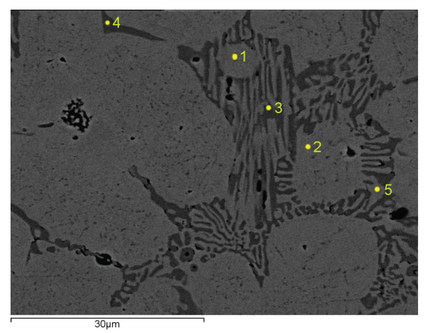
Figure 2.
Microstructure of sample II.
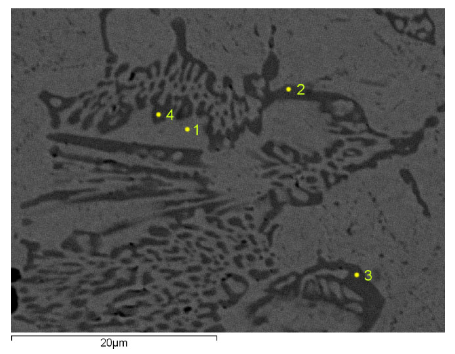
Figure 3.
Microstructure of sample III.
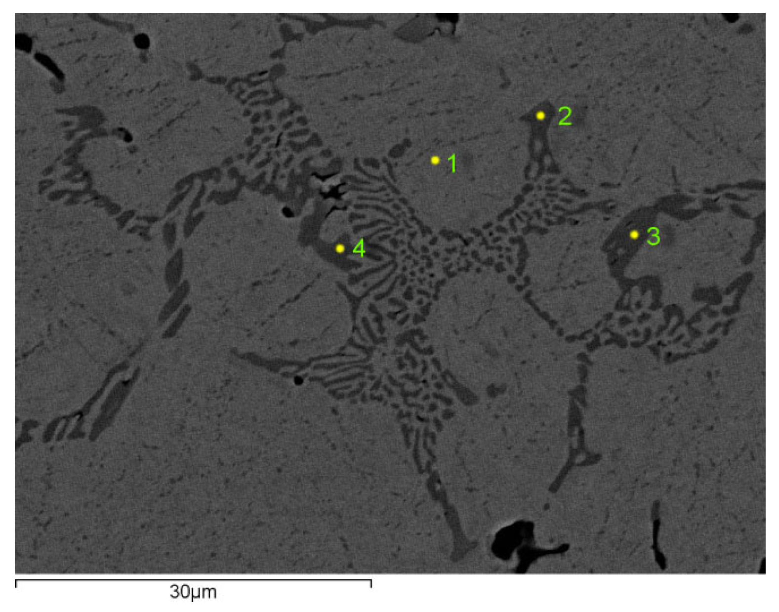
Figure 4.
Microstructure of sample IV.
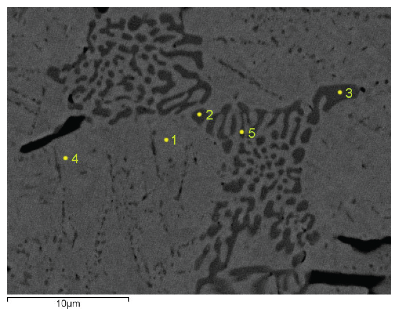
Figure 5.
Elements distribution maps in sample IV.
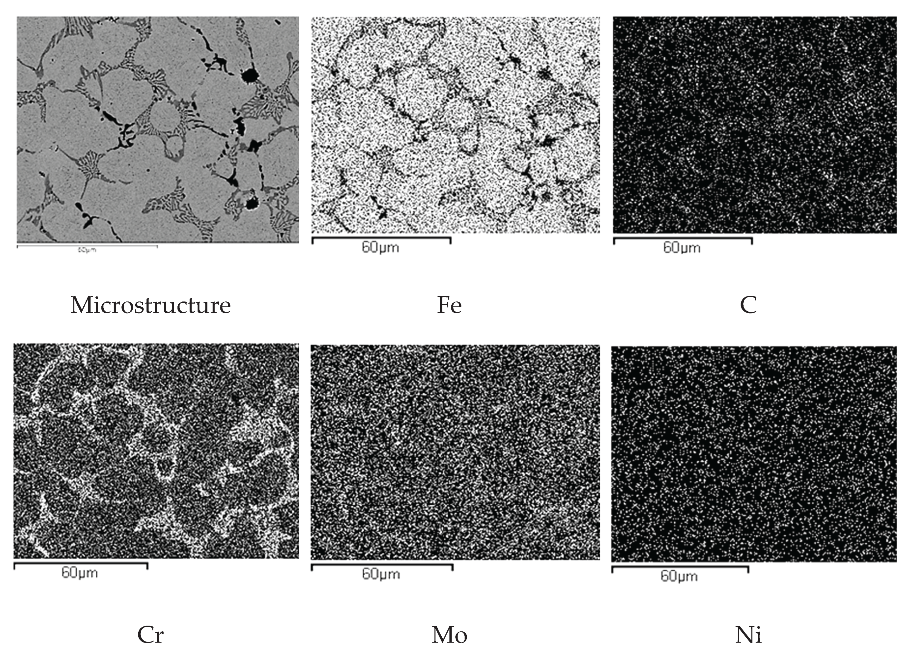
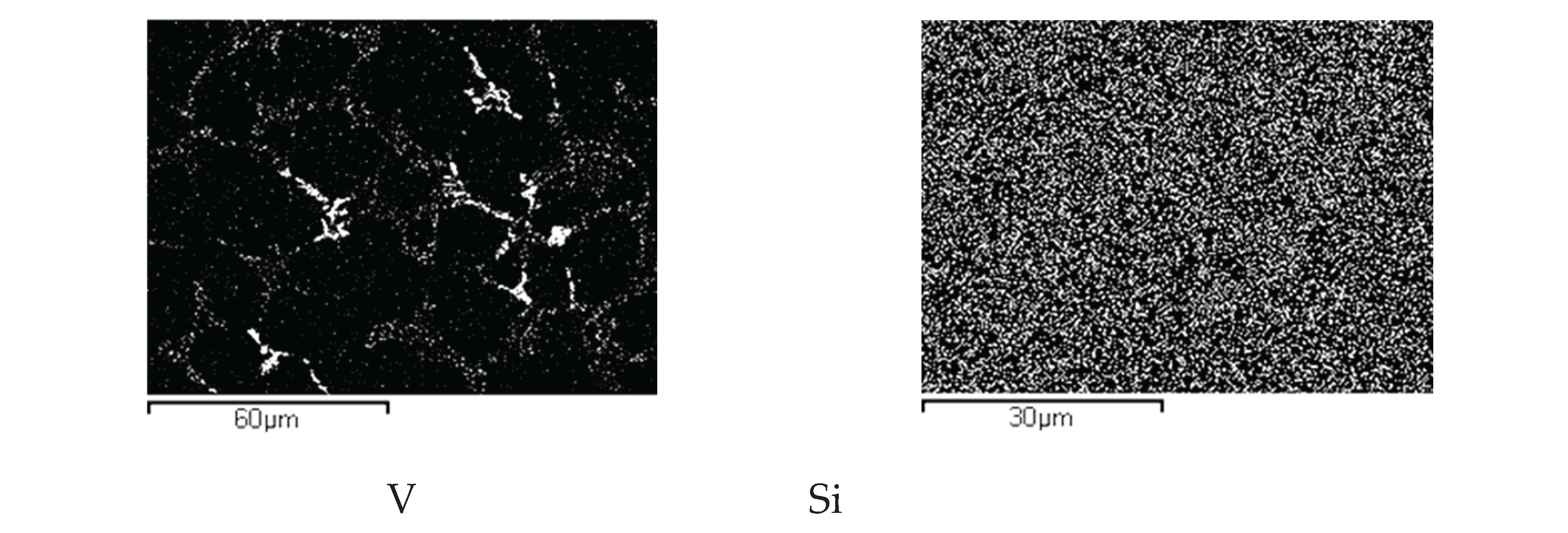
Figure 6.
The diffractogram for tested sample IV.
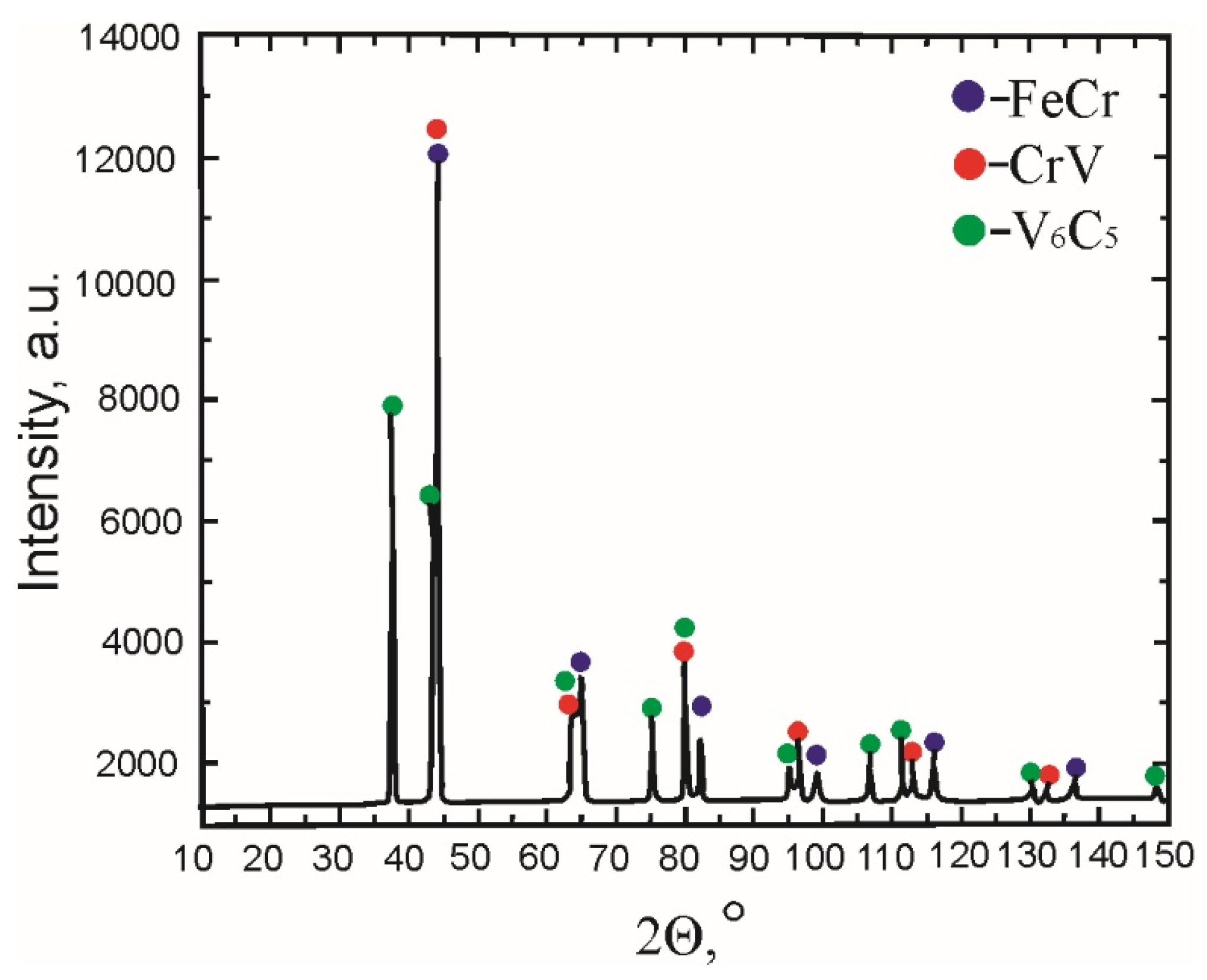
Figure 7.
Mean values of friction coefficients for each sample.
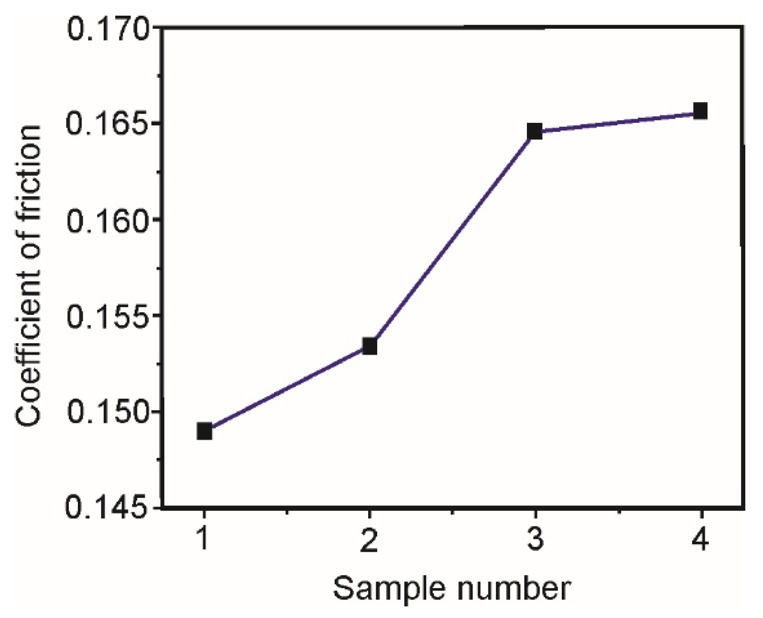
Figure 8.
Mean values of the wear traces’ surface, μm2 for each sample.
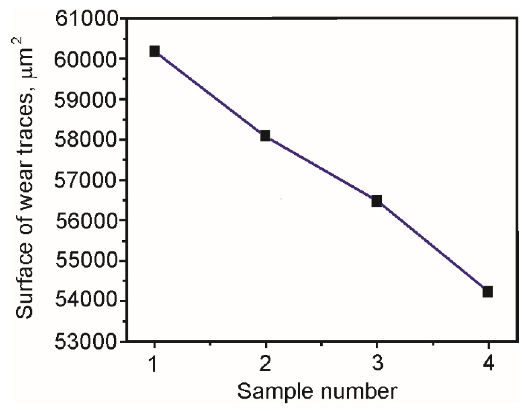
Figure 9.
Mean values of the worn material volume for each sample.
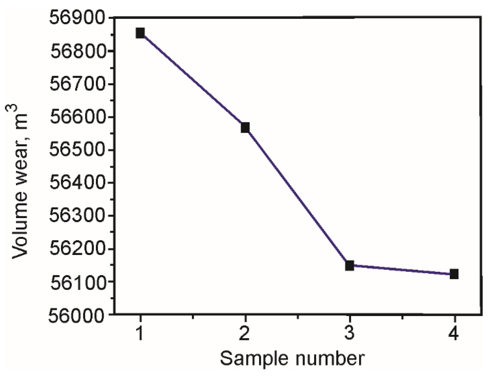
Figure 10.
Magnified view of the alloy I wear trace.
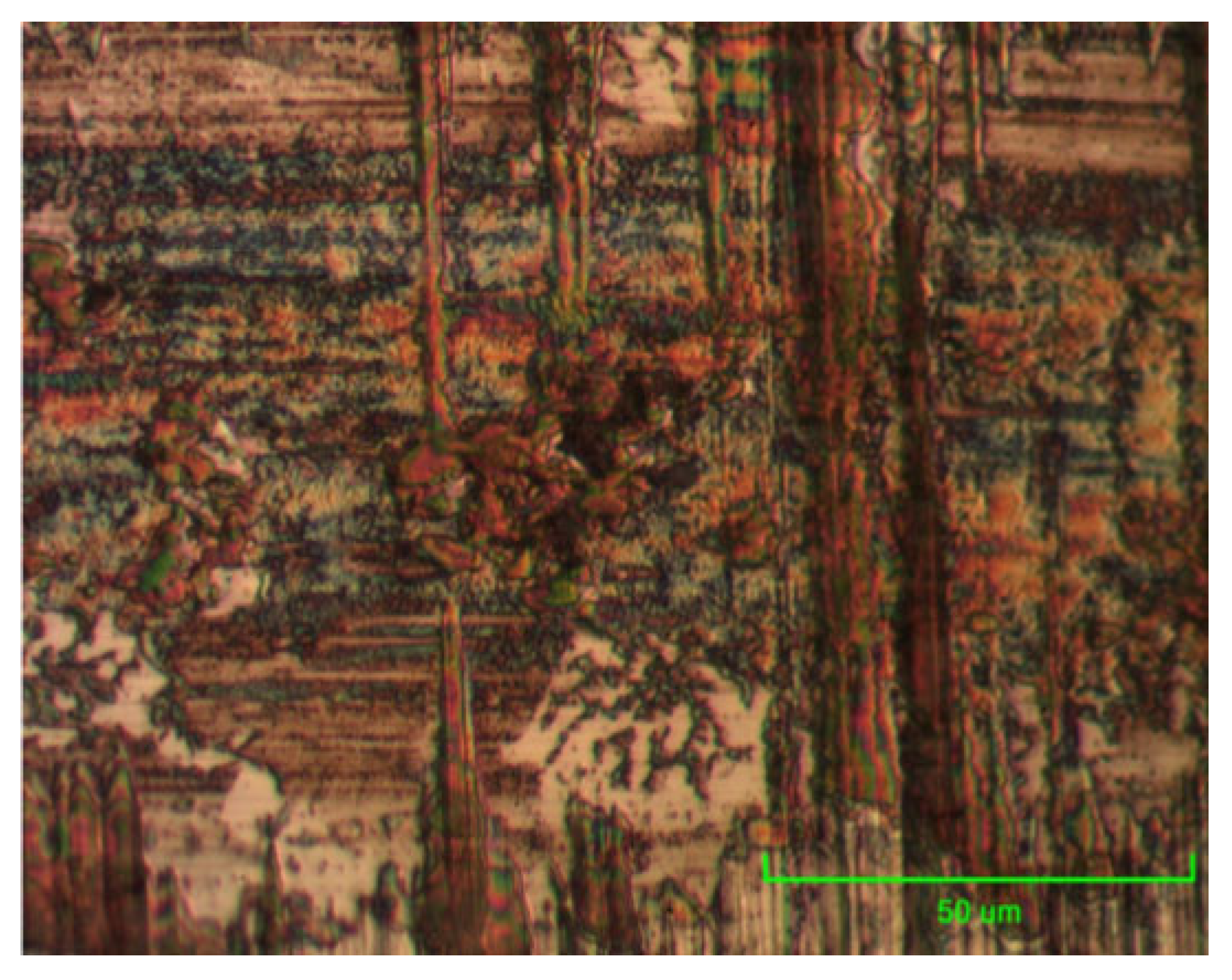
Figure 11.
Appearance of the ball wear: (a) with wear products and (b) without wear products.
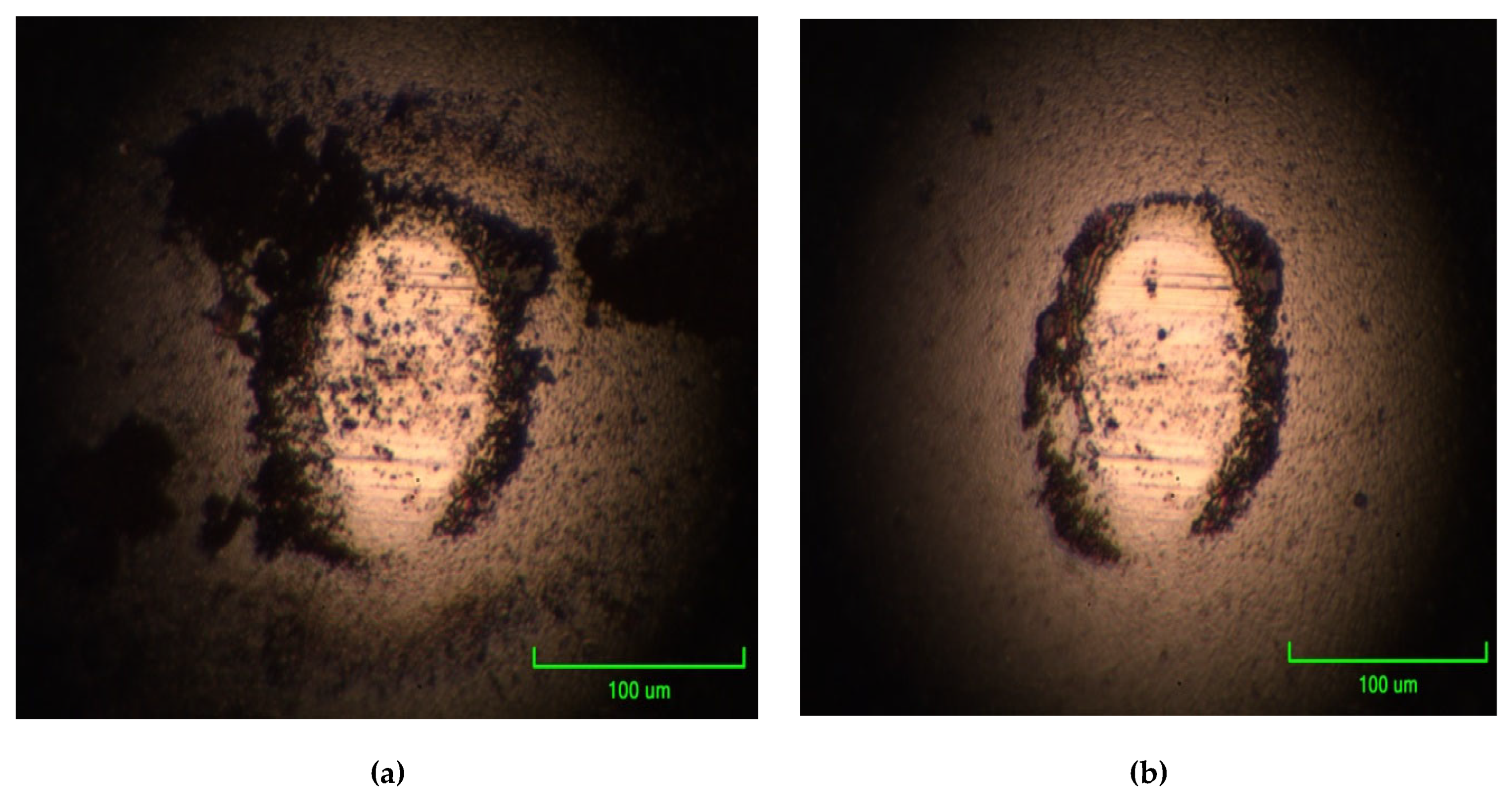
Figure 12.
Open circuit potential for samples I, II, III and IV in 0.1 M H2SO4.
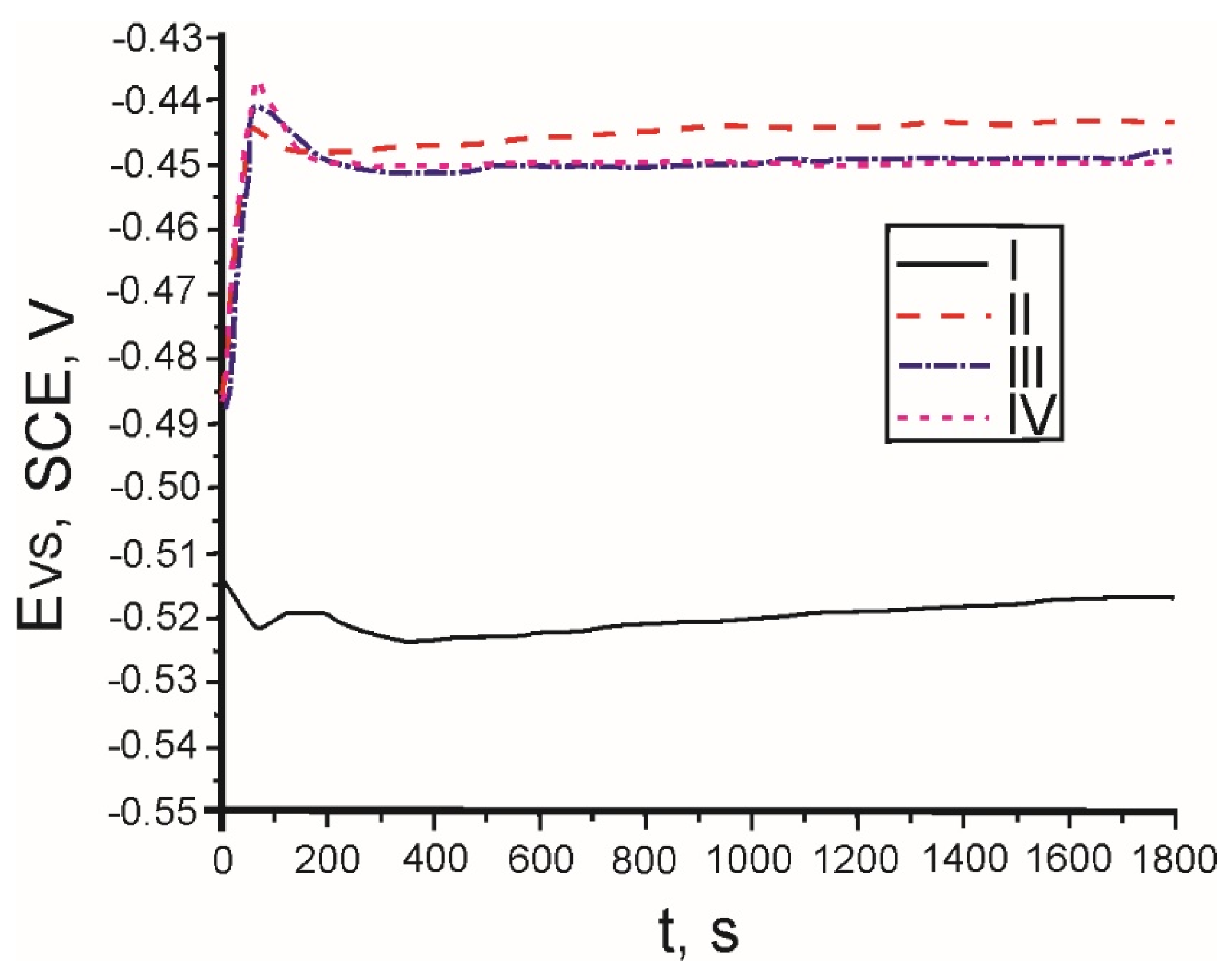
Figure 13.
Cyclic voltammetry diagrams of samples I to IV in acidic environment.
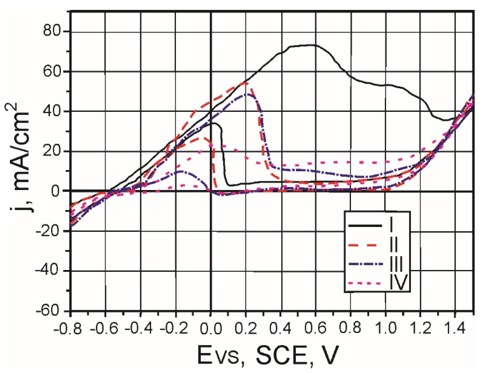
Figure 14.
Open circuit potential for samples I, II, III and IV in 0.1 M NaCl.
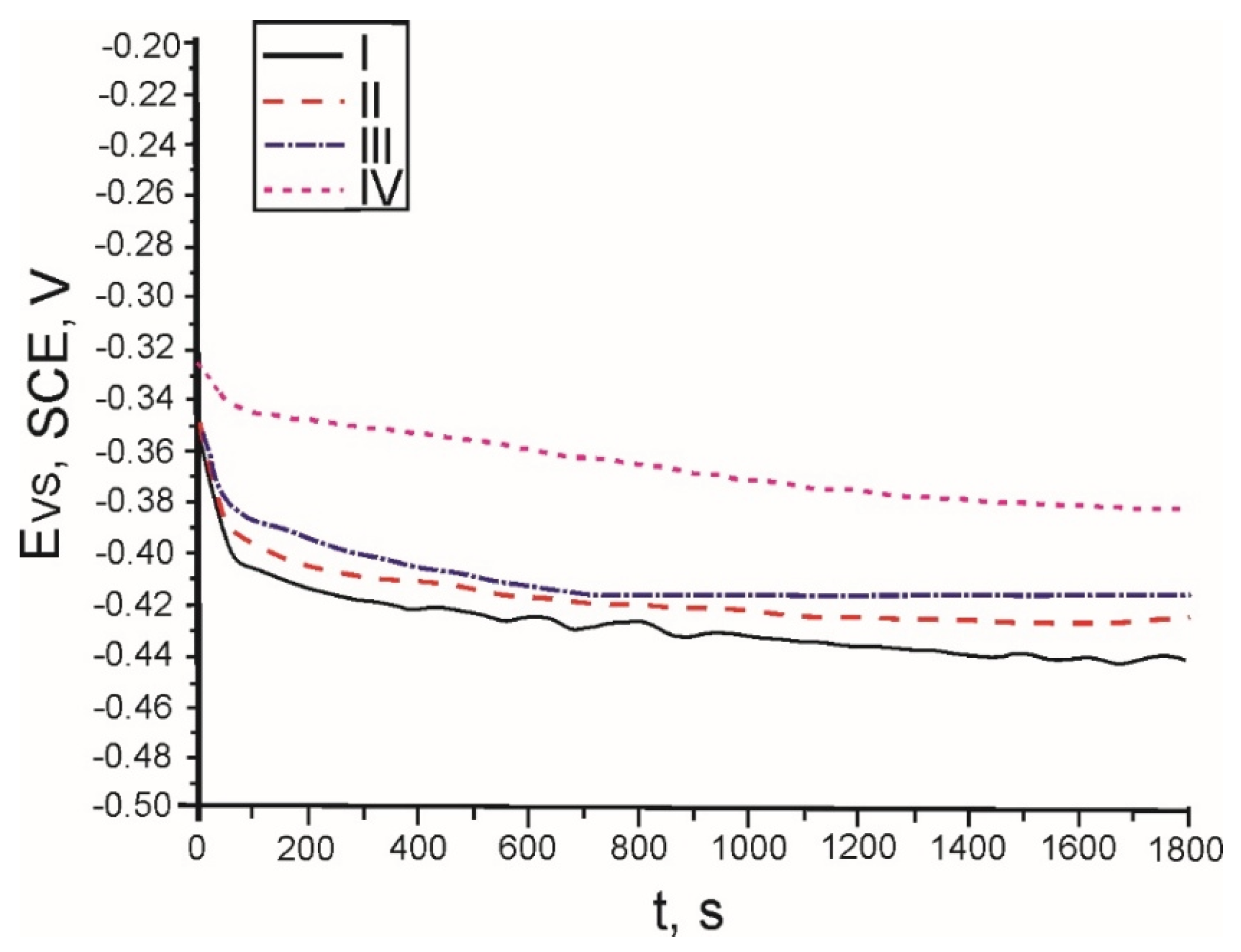
Figure 15.
Cyclic voltammograms obtained on samples I to IV in a neutral environment.
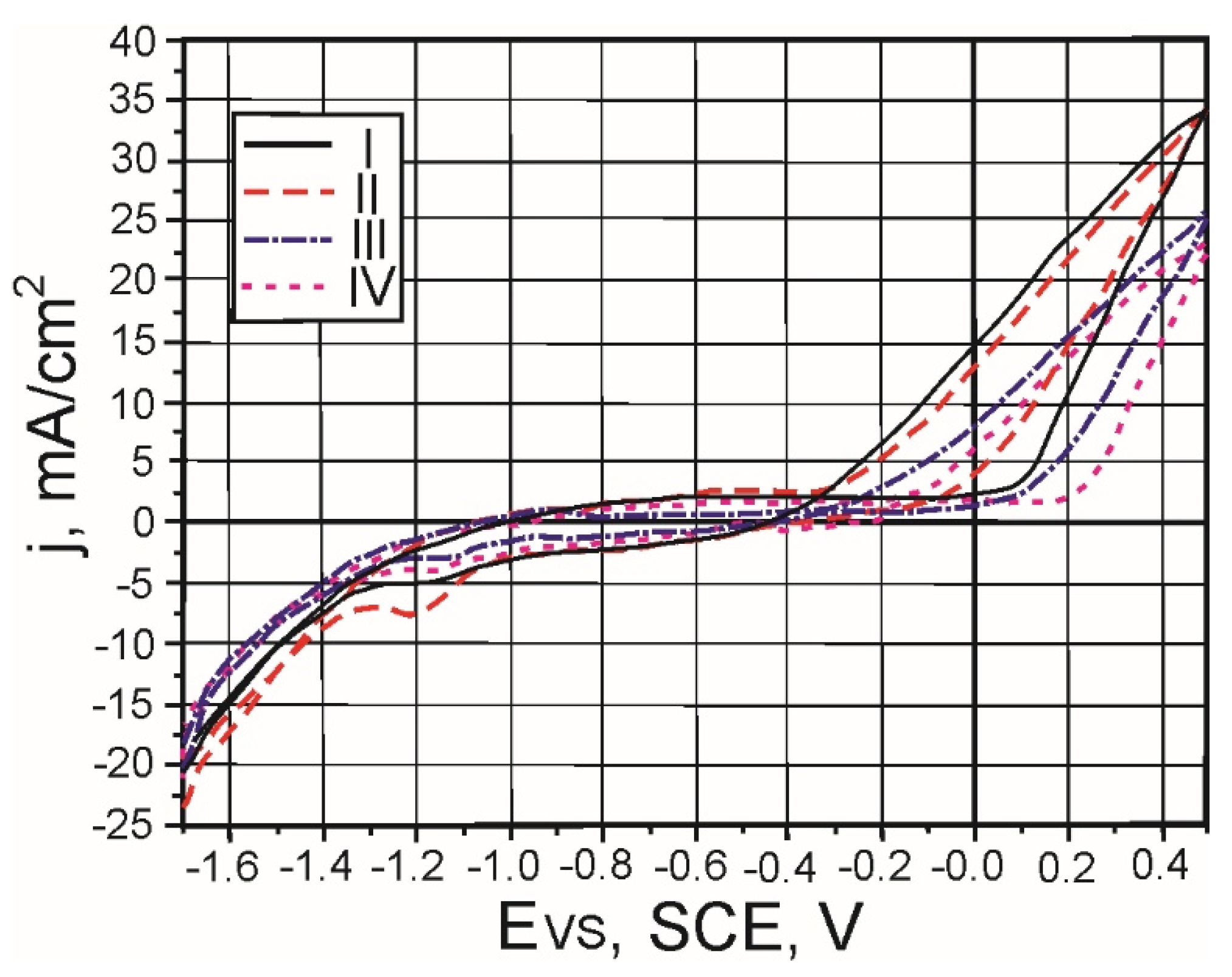
Figure 16.
Open circuit potential for samples I, II, III and IV in 0.1 M NaOH.
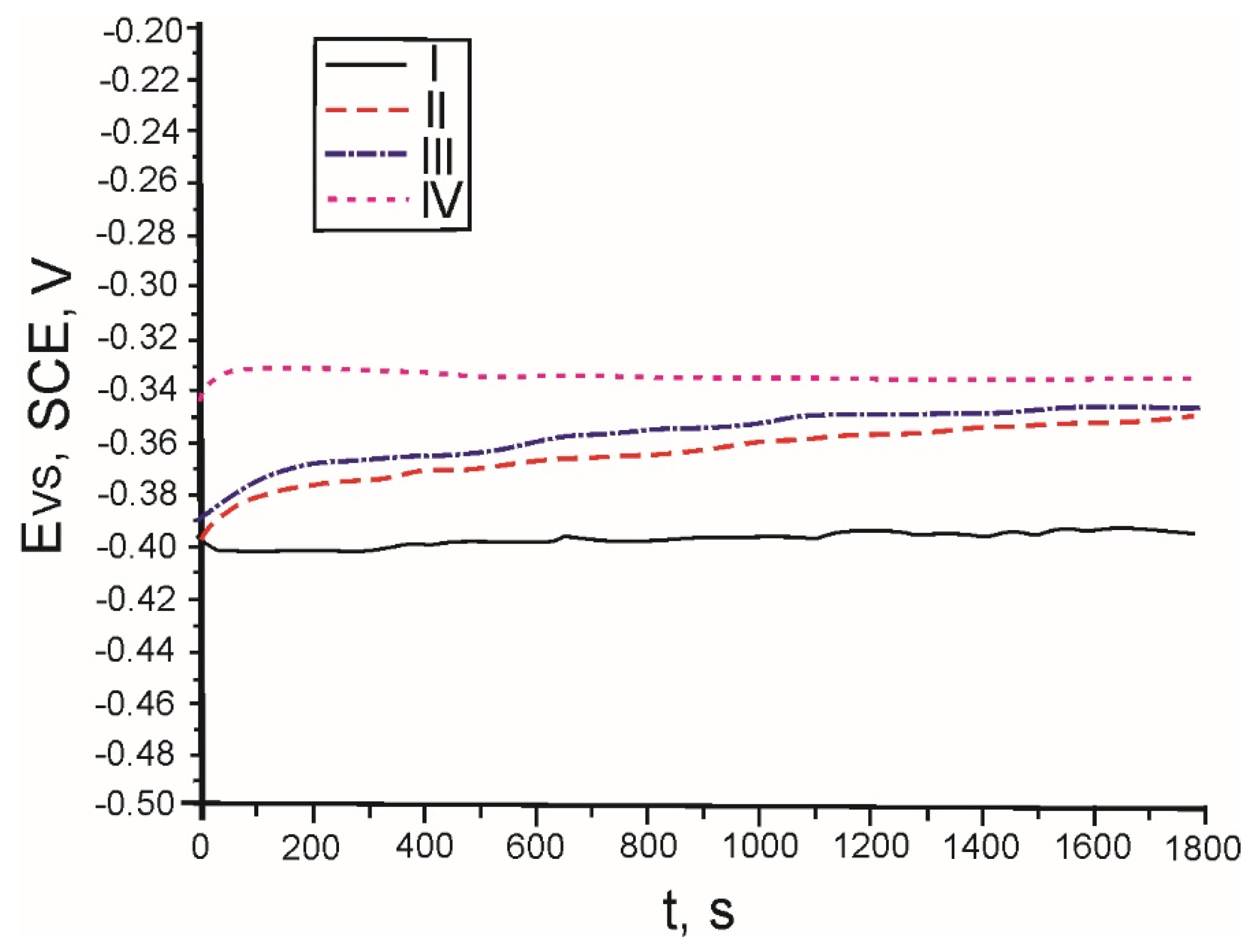
Figure 17.
Cyclic voltammograms obtained on samples I to IV in alkaline medium.
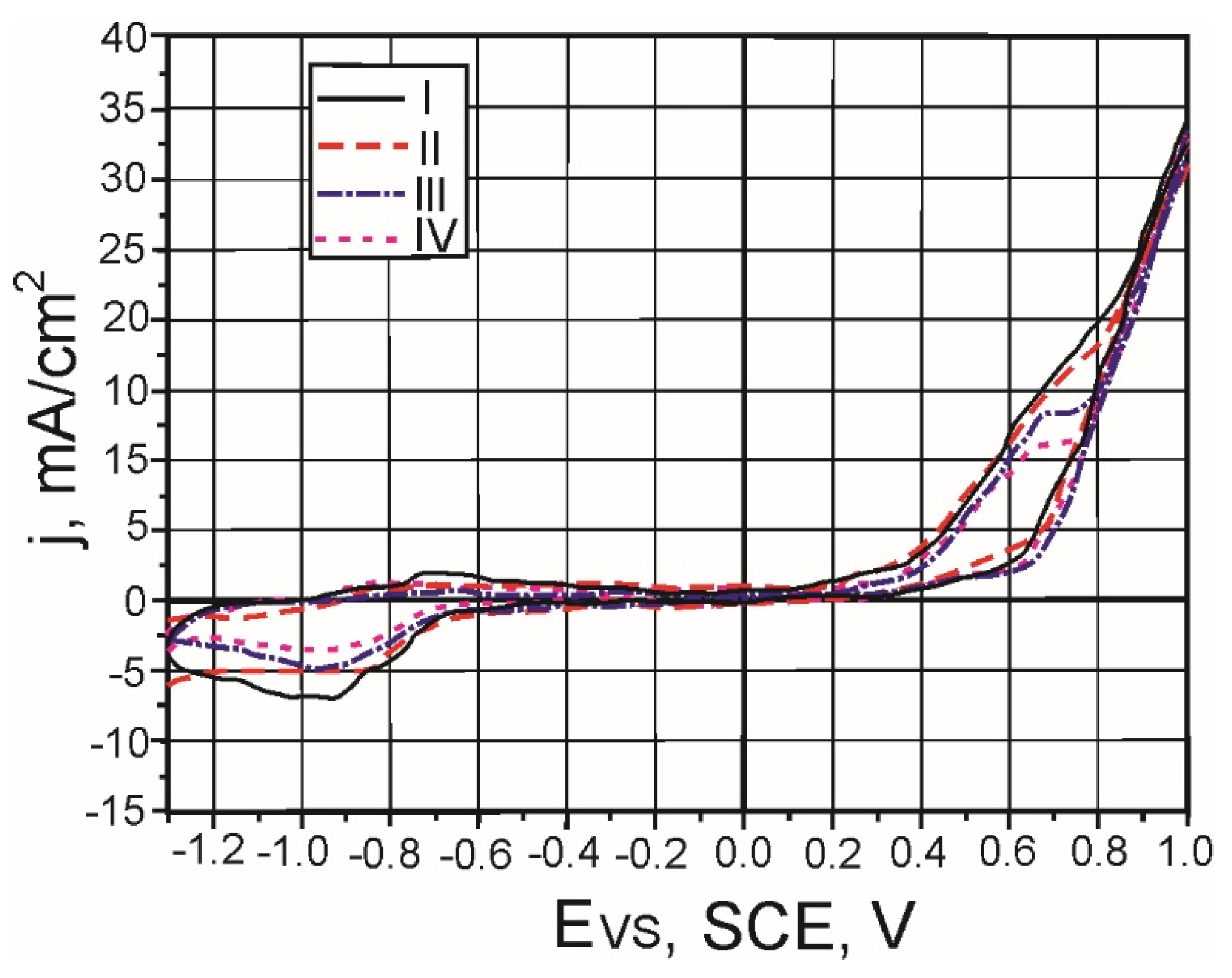
Table 1.
Chemical composition of the X189CrMo12-1 steel, wt %.
| C | Cr | Mo | S | Si | P | Mn | Al | Ni | V |
| 1.8 | 12 | 1.0 | 0.03 | 0.50 | 0.034 | 0.5 | 0.02 | 0.2 | 0.502 |
Table 2.
Chemical composition of all sample series, mass %.
| Sample # | C | Cr | Mo | S | Si | P | Mn | Al | Ni | V |
| I | 1.753 | 11.754 | 1.125 | 0.035 | 0.514 | 0.034 | 0.533 | 0.02 | 0.16 | 0.502 |
| II | 1.711 | 10.524 | 1.130 | 0.033 | 0.514 | 0.033 | 0.524 | 0.01 | 0.15 | 1.006 |
| III | 1.732 | 11.466 | 1.268 | 0.022 | 0.549 | 0.022 | 0.662 | 0.02 | 0.03 | 1.908 |
| IV | 1.699 | 11.236 | 1.248 | 0.020 | 0.540 | 0.021 | 0.650 | 0.02 | 0.01 | 2.835 |
Table 3.
Chemical composition of tested phases of sample I, wt %.
| Point # | C | Si | V | Cr | Fe | Ni | Mo |
| 1 | 9.16 | 0.53 | 1.85 | 12.48 | 74.08 | 0.43 | 1.48 |
| 2 | 3.17 | 0.59 | 1.97 | 11.95 | 81.70 | - | 0.6 |
| 3 | 14.54 | - | 9.21 | 32.91 | 41.15 | - | 2.19 |
| 4 | 15.20 | - | 12.76 | 39.67 | 29.33 | - | 3.04 |
| 5 | 8.76 | 0.50 | 1.680 | 10.53 | 77.49 | - | 1.04 |
Table 4.
Chemical composition of tested phases of sample II, wt %.
| Point # | C | Si | V | Cr | Fe | Ni | Mo |
| 1 | 7.51 | 0.66 | 1.67 | 11.51 | 77.27 | 0.22 | 1.16 |
| 2 | 13.89 | - | 11.14 | 36.02 | 35.51 | 0.31 | 3.13 |
| 3 | 14.37 | - | 12.15 | 37.98 | 32.57 | - | 2.92 |
| 4 | 12.86 | - | 9.09 | 32.27 | 43.40 | - | 2.38 |
Table 7.
Results of the XRD analysis.
| Detected compound | Space group | Pearson symbol | Prototype structure | Latice parameters (Å) |
| FeCr | Imm | cI2 | W | a = b = c = 2.8654(3) |
| CrV | Imm | cI2 | W | a = b = c = 2.9175(1) |
| V6C5 | P3112 | hP33 | V6C5 |
a = b = 5.0913(1) c = 14.4324(2) |
Table 8.
Friction coefficient values of the tested samples.
| Test # | Friction coefficient | ||||
| I | II | III | IV | ||
| 1 | 0.14 | 0.162 | 0.165 | 0.166 | |
| 2 | 0.16 | 0.157 | 0.161 | 0.15 | |
| 3 | 0.143 | 0.146 | 0.171 | 0.17 | |
| 4 | 0.154 | 0.155 | 0.162 | 0.179 | |
| 5 | 0.148 | 0.147 | 0.164 | 0.163 | |
| Average value | 0.149 | 0.1534 | 0.1646 | 0.1656 | |
| Standard deviation | 0.0106 | 0.0078 | 0.0112 | 0.0081 | |
Table 9.
Measured values of the wear traces’ surfaces, μm2 and lengths, μm.
| Test # | Sample # | |||||||
| I | II | III | IV | |||||
| Surface | Length | Surface | Length | Surface | Length | Surface | Length | |
| 1 | 59470.27 | 627.45 | 56452.58 | 606.61 | 53703.47 | 611.4 | 56385.5 | 601.08 |
| 2 | 61611.93 | 649.07 | 62224.57 | 650.98 | 54999.85 | 665.73 | 52356.56 | 601.65 |
| 3 | 62021.62 | 683.75 | 58045.77 | 685.75 | 60174.5 | 686.99 | 52112.12 | 510.94 |
| 4 | 57371.95 | 644.74 | 59510.87 | 691.01 | 54925.06 | 669.18 | 57252.68 | 596.19 |
| 5 | 60434.61 | 672.09 | 54087.61 | 614.36 | 58596.63 | 681.63 | 53074.99 | 577.2 |
| Average value | 60182.08 | - | 58064.28 | - | 56479.9 | - | 54236.37 | - |
| Standard deviation | 1863.844 | - | 3074.592 | - | 2862.299 | - | 1724.498 | - |
Table 10.
Calculated values of the worn material volumes, μm3.
| Test # | Sample # | |||
| I | II | III | IV | |
| 65822.97 | 59431.95 | 55195.74 | 56386.61 | |
| 1 | 56690.60 | 61757.74 | 49351.33 | 64246.69 |
| 2 | 57088.88 | 56763.51 | 67538.6 | 54254.39 |
| 3 | 53829.93 | 50529.64 | 58736.82 | 54091.66 |
| 4 | 50842.54 | 54353.64 | 49918.89 | 51628.82 |
| 5 | 56854.99 | 56567.30 | 56148.28 | 56121.63 |
| Average value | 5608.185 | 4374.328 | 7455.722 | 7114.655 |
| Standard deviation | 65822.97 | 59431.95 | 55195.74 | 56386.61 |
Table 11.
Open circuit rest potentials for different environments.
| Electrolyte | Open circuit rest potential, V | |||
| I | II | III | IV | |
| 0.1M H2SO4 | -0.517 | -0.443 | -0.448 | -0.45 |
| 0.1M NaCl | -0.442 | -0.424 | -0.416 | -0.383 |
| 0.1M NaOH | -0.398 | -0.354 | -0.351 | -0.34 |
Disclaimer/Publisher’s Note: The statements, opinions and data contained in all publications are solely those of the individual author(s) and contributor(s) and not of MDPI and/or the editor(s). MDPI and/or the editor(s) disclaim responsibility for any injury to people or property resulting from any ideas, methods, instructions or products referred to in the content. |
© 2026 by the authors. Licensee MDPI, Basel, Switzerland. This article is an open access article distributed under the terms and conditions of the Creative Commons Attribution (CC BY) license (http://creativecommons.org/licenses/by/4.0/).
Copyright: This open access article is published under a Creative Commons CC BY 4.0 license, which permit the free download, distribution, and reuse, provided that the author and preprint are cited in any reuse.


