Submitted:
20 February 2026
Posted:
26 February 2026
You are already at the latest version
Abstract
Rail trespassing remains a persistent safety challenge at the system level in the United States. However, identifying hot spots proactively is difficult due to limited incident data and strong spatial dependencies within the built environment. This study creates a ZIP-code–level geospatial analytics framework to identify current and emerging trespassing hot spots across North Carolina by combining land-use composition, rail exposure metrics, and historical Federal Railroad Administration (FRA) trespassing records. Geospatial layers were integrated within a GIS workflow to derive predictors such as rail miles, grade crossings, crossings per mile, population density, and land-use types encoded as one-hot vectors. Exploratory spatial analysis showed significant clustering of trespassing incidents, with Global Moran’s I indicating positive spatial autocorrelation across multiple neighborhood sizes. Permutation z-scores confirmed non-random hotspot formation along major rail corridors. A k-means clustering method identified four structural risk environments, and a Cluster Risk Index (CRI) was developed from weighted, standardized exposure and land-use variables to quantify latent risk, independent of raw casualty counts. Results demonstrate that dense urban–industrial rail corridors have the highest CRI values and exhibit the strongest spatial autocorrelation. In contrast, rural ZIP codes with long rail lines show increased exposure-based risk despite fewer historical casualties. The resulting risk surfaces and hotspot classifications provide an interpretable and scalable framework for statewide safety planning, early hotspot detection, and targeted interventions by transportation agencies.
Keywords:
rail trespassing
; spatial autocorrelation
; hot spot analysis
; cluster risk index
; systems modeling
; spatial data
; transportation safety
1. Introduction
Railroad trespassing persists as a significant and perilous issue, causing numerous fatalities, injuries, and operational interruptions globally. In the United States, trespassing on railroads results in hundreds of deaths annually, representing a considerable proportion of rail-related casualties [1]. Despite increased awareness and ongoing safety initiatives, the prevalence of railroad trespassing continues to be a serious public safety concern. While behavioral and demographic aspects are commonly investigated in relation to trespassing, the physical and spatial environment where these incidents occur has received less scrutiny. According to literature, the built and natural environment—including elements such as pedestrian crossings, fencing, land use, and proximity to rail tracks—significantly influences the likelihood of trespassing[2,3]. However, comprehensive investigations of these spatial correlations, particularly through geographic information systems, remain limited. Most existing studies rely on aggregated data or anecdotal evidence, providing little insight into the micro-level characteristics that elevate the probability of trespassing occurrences. There is a critical need for location-specific, data-driven analyses that incorporate spatial and environmental attributes to enhance the effectiveness of prevention strategies. Spatial correlation refers to the degree to which observations located near one another exhibit similar values, reflecting the spatial dependence described by Tobler’s First Law of Geography [4]. It is commonly quantified using global or local measures such as Moran’s I [5], Geary’s C [6], or Local Indicators of Spatial Association (LISA) statistics [7].
This study addresses this need by investigating the relationship between the physical characteristics of the railroad environment and the spatial distribution of trespassing incidents. Utilizing GIS data and advanced spatial modeling methods, this research identifies high-risk locations based on established environmental features and constructs a classification model for identifying trespassing hot spots. By employing spatial analysis and machine learning methodologies, this study aims to go beyond retrospective analysis and support proactive safety planning. The primary objectives of this study are: (1) analyze the spatial distribution of railroad trespassing incidents within a defined geographical area, in this case, North Carolina, USA. (2) identify the physical and environmental factors most closely associated with these incidents, and (3) develop a predictive hot spot model to aid rail authorities in targeting preventive measures. Ultimately, the findings are expected to facilitate more effective, geographically targeted interventions, decrease trespassing-related injuries and fatalities, and contribute to the expanding body of knowledge on spatial risk modeling in transportation safety. The next section discusses previous studies that have used these techniques in different contexts. Subsequent sections provides details of the methodology employed in this study as well as the results of the analysis and their implications for transportation safety policy.
2. Literature Review
Railroad trespassing poses a persistent and complex challenge, endangering individuals, disrupting rail services, and jeopardizing public safety. Understanding its root causes is crucial for developing effective prevention strategies [8]. Research highlights a complex interplay of factors—primarily, railroad infrastructure design, surrounding land use, and human activity patterns as key drivers of trespassing incidents [9]. Silla & Luoma [10] found that residents near tracks often lack sufficient legal crossings, necessitating trespassing, especially in districts where homes are separated from city centers by railroad lines. Furthermore, commercial areas near stations often experience higher rates of crime, including trespassing, although with different patterns than residential areas, varying by day and time [11].
Geographic Information Systems (GIS) provide a comprehensive framework for managing and analyzing spatially referenced data, enabling researchers to examine geographic patterns and relationships across multiple scales [12]. GIS have been extensively utilized in transportation safety for various purposes, including risk mapping and hot spot prediction. Li et al.[13] for instance uses GIS to display locations of intra-city motor vehicles crashes as well as the hot spots. Bilim[14] similarly uses the same tool for spatial autocorrelation and kernel density estimation to obtain the distribution and identification of the most critical locations for pedestrian road crashes. GIS techniques such as Kernel Density Estimation (KDE), Getis-Ord Gi*, and Moran’s I have proven useful in identifying accident-prone areas and hot spots by aiding in clustering accidents and identifying black spots which are crucial for planning and safety interventions [15,16]. By combining physical data such as infrastructure layouts, topography, and land use with human-related data, including population density, behavioral patterns, and socioeconomic indicators, GIS facilitates a comprehensive understanding of the factors contributing to risks in a given area. This integrative capacity makes it possible to analyze how environmental and human variables interact to create or exacerbate hazardous conditions. Moreover, GIS enhances decision-making processes by offering detailed, location-specific insights into potential hazards, areas of vulnerability, and high-risk zones [17].
Regarding predictive modeling, Generalized Linear Models (GLMs), particularly those employing the negative binomial distribution, are commonly used to analyze count data such as crash frequencies. These models are especially suited for handling overdispersion, a frequent characteristic of crash data. To further enhance the predictive power and account for spatial characteristics inherent in safety data, researchers have increasingly integrated spatial regression techniques. Notably, methods such as Geographically Weighted Poisson Regression (GWPR) and Geographically Weighted Negative Binomial Regression (GWNBR) have been applied to capture spatial dependency and heterogeneity in crash occurrences [18]. These approaches allow model parameters to vary across geographic space, thus providing localized insights that traditional global models may overlook.
In addition to geographically weighted models, spatial smoothing techniques such as the Intrinsic Conditional Autoregressive (CAR) model and its widely used extension, the Besag–York–Mollié (BYM) model, have proven effective. These models "borrow strength" from neighboring areas to stabilize estimates in regions with sparse data, thereby improving the reliability of spatial predictions and addressing issues related to spatial correlation and unobserved heterogeneity [19]. Furthermore, geographic machine learning methods are gaining traction for their ability to handle complex, non-linear relationships among spatial predictors. Techniques such as localized Support Vector Regression (SVR) have been employed to perform spatially-aware feature selection and to quantify the relative importance of predictor variables. For instance, Duong & Nguyen [20] demonstrated the use of local SVR in a spatial safety study to identify key risk factors influencing crash occurrences, highlighting the method’s utility in refining predictive accuracy and uncovering localized patterns in traffic risk.
2.1. Research Gap
Although railroad trespassing is increasingly recognized as a significant safety concern, current research predominantly emphasizes behavioral, demographic, or temporal dimensions, with inadequate consideration of physical and spatial determinants. Existing spatial analysis often provide descriptive insights but fail to integrate data pertaining to physical infrastructure, such as access routes, barriers, land utilization, or adjacency to urban areas. This deficiency curtails a holistic understanding of how the built environment influences trespassing incidents, thereby impeding the formulation of targeted preventative measures. Furthermore, the application of predictive modeling within a GIS to forecast potential hot spots based on environmental attributes remains limited. This study addresses these limitations by synthesizing granular spatial data with predictive analytical techniques to identify physical factors correlated with trespassing and to produce actionable hot spot maps. By merging physical infrastructure characteristics with geospatial behavioral patterns, this research promotes a more holistic and forward-thinking strategy for railroad safety management.
3. Methodology
To achieve our research objectives, we develop a spatially explicit, ZIP–code–level prediction model that identifies current and emerging railway trespassing hot spots across North Carolina. The methodological framework integrates geospatial data processing, exploratory spatial analysis, and cluster-based risk characterization for hotspot prediction.
3.1. Study Area Description
Situated in the southeastern United States, North Carolina features a complex rail network that extends across diverse urban, suburban, and rural terrains. The state’s railroad infrastructure (Figure 1) is crucial for both freight and passenger transport, incorporating over 3,600 miles of active lines managed by Class I railroads, regional carriers, and short-line operators [21]. Key rail corridors link major urban centers, including Charlotte, Raleigh, Greensboro, and Wilmington, while smaller branch lines serve industrial, agricultural, and rural sectors. This network, characterized by both high-traffic urban sections and isolated rural tracks, offers a varied geographical context for studying railroad trespassing patterns.
The diverse land use patterns surrounding North Carolina’s rail segments—ranging from dense residential and commercial zones to forested and agricultural areas—provide an optimal setting for investigating the influence of physical and environmental characteristics on trespassing behavior. Many rail segments lack adequate physical barriers, such as fencing or controlled crossings, increasing the likelihood of unauthorized access in certain areas. Additionally, the proximity of rail lines to urban schools, homeless encampments, recreational paths, and transit stations heightens the potential for pedestrian interaction with railroad environments. These spatial and infrastructural variations across the state offer a unique opportunity to examine how physical context contributes to trespassing risk.
This study includes all accessible rail segments within North Carolina, utilizing geospatial data from North Carolina Department of Transportation (NCDOT), Federal Railroad Administration (FRA) trespassing incident records, and supplementary spatial layers like land use and demographic overlays. The statewide scope allows for a comprehensive analysis that considers regional differences in rail environments, providing broader insights into trespassing risk factors beyond specific hot spots. By analyzing spatial patterns and environmental correlates at the state level, this study seeks to inform more effective, geographically targeted safety measures for preventing railroad trespassing.
3.2. Data Sources and Preprocessing
Data on railroad trespassing casualty is obtained from the Federal Railroad Administration (FRA) Injury and Illness Summary database [23]. This dataset includes detailed information for each recorded event, such as geographic coordinates, location descriptions, and the exact date and time of occurrence, among other variables. Geo-coding of incidents didn’t start until 2011 therefore our analysis uses data from 2011 to 2024. To complement this, data on all public and private grade crossings across the state of North Carolina are sourced from the US Department of Transportation (USDOT) database [24]. The crossing dataset provides additional attributes, including the designated purpose of each crossing (e.g., vehicular, pedestrian), geographic coordinates, associated street names, and the managing railroad company.
3.3. Spatial Autocorrelation Using Moran’s I
Moran’s I is a widely recognized and utilized method for quantifying spatial autocorrelation, serving as a vital tool in various disciplines including transportation safety to ascertain the degree to which values of a variable such as trespassing incidents spots are clustered together in space [25]. Thus, this procedure is used to answer the first research question: How are railroad trespassing incidents spatially distributed across North Carolina, and what geographic patterns or clusters emerge within the state?. This statistic assesses whether observed spatial patterns are clustered, dispersed, or random [26,27]. Moran’s I operates on the principle of comparing the similarity of values at different locations with the spatial relationships between those locations [28]. A positive Moran’s I value suggests that similar values tend to cluster together, indicating positive spatial autocorrelation, where high values are located near other high values, and low values are located near other low values [29]. Conversely, a negative Moran’s I value suggests that dissimilar values tend to cluster together, indicating negative spatial autocorrelation, where high values are located near low values and vice versa. A Moran’s I value close to zero indicates a random spatial pattern, suggesting that the values are distributed independently of their locations. The formula for Moran’s I is expressed as:
where N is the number of observations, represents the spatial weight between trespassing locations i and j, is the mean number of incidents across all locations, while represents the number of incidents at location i. The spatial weights matrix defines the spatial relationships between observations and can be based on various criteria, such as adjacency, distance, or other measures of spatial proximity [30]. Moran’s I, in essence, measures the extent to which the presence of a phenomenon in one location influences its presence in neighboring locations [31]. It has been demonstrated that results are dependent on both the number of events in the data and the degree of spatial clustering, so a single ‘appropriate’ scale is not identified [32].
Moran’s I can also be calculated locally, as Local Indicators of Spatial Association, to analyze the spatial autocorrelation in smaller areas [33]. A positive local Moran’s I value for a specific location indicates that the location has neighboring locations with similar values and negative values, on the other hand, indicate that a location has neighboring locations with dissimilar values [34]. The Local Indicators of Spatial Association method breaks down global indicators into individual components, illuminating the contribution of each observation to the total, and evaluates the degree of spatial clustering by pinpointing significant clusters or outliers [35]. These can be visualized in cluster maps.
3.3.1. Data Description
We compiled a ZIP-code–level dataset for North Carolina (N = 766 ZIP polygons) to quantify and map spatial patterns in rail-trespassing harm. Trespassing casualty events were geocoded as points and aggregated to ZIP polygons via a point-in-polygon join to obtain a count of events per ZIP (Casualties). Population denominators (POPULATION) and polygon area in square miles (SQMI) were used to construct a population-standardized outcome, the trespassing casualty rate per 10,000 residents (rate_per_10k = 10,000 × Casualties / POPULATION). ZIPs with zero or missing population (n = 3) were excluded from rate-based statistics to avoid division by zero. Thus, 763 polygons were consequently used. All spatial processing was performed on valid geometries; coordinate reference systems were projected to European Petroleum Survey Group (EPSG) 2264 (USft) for analysis. This ZIP scale was selected to align with corridor/neighborhood phenomena while retaining statewide coverage and sufficient sample size for local spatial statistics. This procedure was done using QGIS ® Desktop version 3.42.3 [36]. Table 1 provides further description of the dataset.
3.4. Hot Spot Classification Model
Predicting future railroad trespassing hot spots is the central objective of this study, aimed at enhancing proactive safety planning and intervention strategies. In developing the model, we also address the second research question: Which physical and environmental factors are most strongly associated with railroad trespassing incidents in North Carolina?. To achieve this, the study utilizes a set of environmental and spatial proximity variables that are hypothesized to influence the likelihood of trespassing behavior. These variables include the level of rail exposure in each zip code (rail miles and number of crossings), population density, and land use composition (e.g., residential, industrial, commercial). Together, these factors provide a rich spatial context that reflects both accessibility and environmental opportunity for trespassing to occur. Areas with limited pedestrian infrastructure are expected to exhibit higher trespassing risk due to the perceived need for shortcuts or lack of alternatives. Land use type offers additional explanatory power by indicating the functional nature of surrounding space. For instance, segments adjacent to residential neighborhoods, informal pathways, or transient spaces such as encampments may exhibit higher vulnerability to unauthorized access. Conversely, areas near commercial zones with controlled access or industrial zones with restricted entry may show different risk patterns.
These environmental and proximity variables are integrated into predictive modeling frameworks such as logistic regression to estimate the probability of future trespassing incidents across the rail network. By training these models on observed incident data and corresponding spatial features, the study identifies patterns and risk factors that generalize beyond known cases. The output of this modeling process includes probability surfaces or risk maps, which highlight potential future hot spots with high spatial resolution. These predictions serve as valuable decision-support tools for railroad authorities, enabling the targeted deployment of surveillance, signage, fencing, or community outreach programs in areas with elevated risk. Ultimately, this approach facilitates a shift from reactive incident response to data-informed, preventative safety strategies. Figure 2 summarizes the major methodological components.
3.4.1. Railroad Crossings
Railroad crossing data were obtained from the Federal Railroad Administration (FRA) inventory and prepared to quantify rail–pedestrian interface exposure at the ZIP-code level. The raw dataset contained point-based records of public and private crossings, including attributes related to location, crossing type, and operational status. Initial preprocessing involved filtering the dataset to retain only active and public crossings relevant to the study period and removing duplicate or incomplete records. All crossing locations were converted to the projected coordinate reference system consistent with the rest of the spatial datasets (NAD83 State Plane, ftUS) to ensure spatial alignment and accurate aggregation.
To generate a ZIP-level measure of crossing exposure, the cleaned crossing points were spatially joined to ZIP code polygons. For each ZIP code, the total number of crossings was computed by counting the number of crossing points falling within its boundary. This aggregation step produced a single, interpretable variable representing crossing density at the ZIP level. The resulting crossing count variable was subsequently merged with other ZIP-level attributes, including population density, rail mileage, and land-use composition, forming a unified analytical dataset. This prepared crossing metric captures the frequency of potential interaction points between rail operations and roadway or pedestrian traffic and serves as a key explanatory variable in subsequent clustering, hotspot characterization, and predictive modeling analyses.
As seen in Table 2, majority of railroad crossings in the study area are highway crossings, accounting for nearly 99% of all recorded locations. Pedestrian-related crossings—including pathway and station pedestrian crossings—represent a very small fraction of the inventory. This distribution reflects the dominant role of roadway–rail interfaces in the regional rail network and underscores the importance of highway crossings as primary points of interaction between rail operations and public activity. Although pedestrian crossings are relatively rare, their presence may still warrant targeted consideration due to elevated vulnerability associated with pedestrian exposure. Also, highway crossings serve as a alternative legal route for pedestrians in the absence of pedestrian crossings, according FRA safety policy [37].
3.4.2. Rail Mileage Calculation
Rail network data were obtained as polyline features representing active railroad segments and processed in QGIS® to quantify rail exposure at the ZIP-code level. All rail geometries were first projected to NAD83 State Plane, ftUS to ensure accurate length calculations. The rail layer was then spatially intersected with ZIP code polygon boundaries, resulting in segmented rail line features corresponding to individual ZIP codes. For each intersected rail segment, geometric length was calculated in feet and subsequently converted to miles. Rail miles were then aggregated by ZIP code by summing the lengths of all rail segments within each ZIP boundary. This procedure produced a continuous ZIP-level rail mileage variable representing the total extent of railroad infrastructure present within each ZIP code. The resulting rail mileage measure was merged with other ZIP-level land-use, and safety variables and used as a key exposure indicator in subsequent analysis.
3.4.3. Land Use Composition
Land-use composition was derived using polygon-based land-use data processed in QGIS® to quantify the spatial distribution of land-use categories within each ZIP code. Land-use polygons were first intersected with ZIP code boundaries, producing subdivided land-use features representing the portion of each land-use category contained within individual ZIP codes. Following the intersection, the area of each land-use polygon segment was calculated in square feet. For each ZIP code, land-use areas were aggregated by category and divided by the total ZIP code area to compute proportional land-use coverage. This process yielded percentage measures of residential, commercial, industrial, agricultural, and other land-use types for each ZIP code. The resulting land-use composition variables capture contextual environmental characteristics and were subsequently integrated with rail infrastructure, demographic, and safety data for use in clustering, hotspot characterization, and predictive modeling analyses. Proportional land-use metrics were employed to ensure comparability across ZIP codes of varying size and to capture the relative dominance of land-use types relevant to contextual exposure and risk. This approach is consistent with prior transportation and land-use research [38,39], which has shown that relative land-use composition better explains travel behavior, exposure patterns, and safety outcomes than absolute measures.
Table 3 presents an illustrative sample of the final ZIP-level prediction dataset used for the hot spot classification model. The dataset integrates demographic characteristics, rail infrastructure exposure, safety outcomes, and proportional land-use composition for each ZIP code. The sample highlights substantial heterogeneity across ZIPs, ranging from dense urban areas with extensive rail infrastructure and multiple casualties to predominantly agricultural ZIPs with minimal rail exposure and no recorded incidents. This example dataset is provided for demonstration and methodological illustration purposes.
4. Results of Spatial Autocorrelation
4.1. Global Spatial Autocorrelation
Global Moran’s I measures the overall spatial dependence in a numeric variable y observed on n spatial units with weights . Using row-standardized weights (), we compute
Positive I indicates that neighboring units tend to have similar values (positive autocorrelation), negative I indicates dissimilarity (checkerboard), and for a random pattern the expectation satisfies .
Weights. k-nearest neighbors (KNN) (k = 10) with row standardization was used to ensure connectivity and comparable neighbor influence across ZIPs. Sensitivity was assessed at .
Hypothesis.
: No spatial autocorrelation (spatial randomness); y is exchangeable across locations.
:positive autocorrelation exists; one-sided
Permutation inference. A conditional randomization test with 999 permutations was performed using the following procedure:
- 1.
- Holding the spatial topology (the weight matrix W) fixed.
- 2.
- Randomly permuting y across locations to generate the reference distribution of I under .
- 3.
- Computing a pseudo p-value as the proportion of permuted statistics at least as extreme as the observed I (tail per the chosen alternative). With 999 permutations, the minimum attainable p-value is .
- 4.
- And finally report I, the permutation-based p-value, and a z-score from the permutation distribution.
The incident rate data was exported as a geopackage and analyzed with GeoPandas, libpysal, and esda in a Python environment using Anaconda® [40]. Global Moran’s I for trespassing casualty rate (per 10,000 population) using KNN (k=10), row-standardized weights, and 999 permutations indicated positive spatial autocorrelation (I = 0.101, z = 7.025, p = 0.001). Also the mean distance to the 10th neighbor is 80,849.1 ft, equivalent to approximately 15.3 miles.
The Moran’s I values in Table 4, as well as the k-sweep plots (Figure 3 and Figure 4) illustrate how the global autocorrelation signal varies with the neighborhood definition. Moran’s I declines from about at to about at , as larger k smooths local contrasts by averaging over more neighbors. In contrast, the permutation z-score generally increases with k (rising from at to – by –20), indicating that—even as the effect size becomes more conservative—the statistic remains highly atypical under spatial randomness and thus strongly significant across all reasonable k. Together, the plots imply a robust, modest positive autocorrelation. The precise magnitude of I depends on k, but the inference ( throughout) is stable. Thus, offers a balanced neighborhood size (local enough to preserve corridor structure, large enough to avoid isolated units), with corroborating sensitivity at and .
4.2. Local Indicators of Spatial Association (LISA)
This section uses Local Moran’s I to move from the global question—does clustering exist?—to the local question—where, exactly, are the clusters and spatial outliers? For each ZIP, we evaluate the trespassing casualty rate per 10,000 residents against the rates of its neighbors, using k-nearest neighbors (k=10) with row-standardized weights to represent local spatial context. Significance is obtained by permutation testing (999 permutations) for each unit; because many tests are run simultaneously, we control the false discovery rate (FDR, ). The resulting LISA map classifies places as High–High (HH) and Low–Low (LL) clusters—interpreted as hotspots and cold spots—alongside High–Low (HL) and Low–High (LH) spatial outliers that may indicate emerging risk or protective pockets. These outputs guide prioritization such as engineering, enforcement, or education and provide a basis for robustness checks such as alternative k, distance bands, or exposure metrics such as per rail-miles or per crossing).
4.2.1. LISA Cluster Counts (FDR-Based)
Applying Local Moran’s I with k-nearest neighbors (), row-standardized weights, and 999 permutations, we controlled for multiple testing using the Benjamini–Hochberg false discovery rate (FDR, ). The resulting classification shows that the majority of ZIP codes were not significant (ns = 483), indicating no detectable local association after correction. A sizeable set formed low–low clusters (LL = 244), i.e., areas with lower rates surrounded by similarly low neighbors (cold spots). In contrast, high–high clusters (HH = 13) were relatively rare but represent the most defensible hot spots—locations with elevated rates embedded within high-rate neighborhoods. We also observed a small number of spatial outliers: low–high (LH = 21), suggesting comparatively low-rate ZIPs adjacent to high-rate neighbors (potential protective pockets), and high–low (HL = 2), indicating isolated high-rate ZIPs amid low-rate surroundings (possible emerging hot spots). Overall, these counts imply that while most of the state does not exhibit significant local association after FDR adjustment, a compact set of hot spots and a narrow band of outliers merit targeted investigation.
As presented in Figure 5, values to the right (positive Local Moran’s I) indicate locations that resemble their neighbors (clustering), while negative values would indicate spatial outliers. Points higher on the plot have smaller permutation p-values (greater statistical evidence). The orange, annotated points identify ZIPs that form High–High clusters after FDR adjustment; these represent the most defensible hot spots where elevated trespassing casualty rates are embedded within similarly high-rate neighborhoods. Most ZIPs cluster near with lower , indicating no detectable local association after multiple-testing correction, consistent with a sparse landscape punctuated by a compact set of statistically significant hot spots. Further details regarding the ZIPs that form high–high clusters is summarized in Table 5.
4.3. Sensitivity Analysis
To assess robustness to the neighborhood definition, we repeated the global test with k-nearest-neighbor weights over . Results were stable: Moran’s I ranged from 0.095–0.114 (k=8: , , ; k=10: , , ; k=12: , , ), indicating a consistent, modest positive spatial autocorrelation irrespective of reasonable changes in k. As expected, larger k slightly smooths local variation and reduces I, but significance remains unchanged. In local analyses (LISA), cluster detection proved more sensitive to k and multiple-testing control: with FDR at , k=10 yielded a small set of hot spots (HH = 13), whereas k=8 and k=12 produced no FDR-significant clusters despite similar raw () patterns. Accordingly, we report k=10 (row-standardized) as the primary specification and include k=8/12 and raw vs. FDR-adjusted results as sensitivity checks. Thus, conclusions about the presence of global clustering are robust, while the exact set of local hot spots varies modestly with neighborhood choice and correction method.
Because Gi* is explicitly scale dependent, the choice of distance band (in feet) controls the size of each feature’s neighborhood and, consequently, the hot spot z–scores. Using a primary fixed band of 15 miles (79,200 ft; row-standardized weights; 999 permutations), we identified statistically significant hot spots along the state’s principal rail corridors. As expected, reducing the band emphasizes tighter, more localized clusters and increases the number of cells classified at 99% confidence, whereas enlarging the band smooths local contrast and reduces the number of “bright” cells. Importantly, most of the core hot spots persisted across reasonable bands (10–20 miles), indicating that the inference is robust to neighborhood definition even though the exact extent and confidence of individual cells vary. To align scales across methods, the primary band was selected to approximately the mean distance to the 10th nearest neighbor (i.e., comparable locality to the LISA analysis with ). Consequently, locations that remain hot at multiple bands are treated as the highest-confidence targets for intervention. Figure 6 and Figure 7 provides a visualization of the contrast between the global intensity hot spots (Gi*) and local similarity clusters (LISA).
5. Results of Hot Spot Classification Model
5.1. Cluster Analysis
K-means clustering was applied to classify ZIP codes into distinct contextual typologies based on rail infrastructure exposure, population density, and land-use composition. The clustering variables included rail miles, number of crossings, population density (POPU_SQMI), and proportional land-use measures (Pct_Residential, Pct_Commercial, Pct_Industrial, and Pct_Agric). All variables were standardized prior to clustering to ensure equal contribution to the distance metric.
The optimal number of clusters was determined using the elbow method, which evaluates the within-cluster sum of squares (inertia) as a function of the number of clusters. As shown in Figure 8, inertia decreases sharply as the number of clusters increases from k = 1 to k = 4, after which the rate of improvement diminishes substantially. This inflection point indicates that additional clusters beyond k = 4 yield only marginal reductions in within-cluster variance. Based on this pattern, a four-cluster solution was selected as the most parsimonious and interpretable representation of the data. A silhouette score of 0.63 was obtained, which indicates strong cluster cohesion and separation, supporting the robustness and interpretability of the selected k-means clustering solution.
Table 6 represents cluster centroids which were computed as the mean values of the standardized clustering variables for each k-means group and subsequently back-transformed to original units for interpretability. Each centroid therefore characterizes the typical rail exposure and land-use profile of ZIP codes within a given cluster. The four clusters exhibit clear and meaningful differences in rail exposure, population density, and land-use composition. Cluster 0 is characterized by very low rail mileage and few crossings, relatively low population density, and a high proportion of agricultural land use, representing predominantly rural, low-exposure ZIP codes. Cluster 1 reflects suburban or peri-urban ZIP codes with moderate rail mileage and crossings, mixed residential and industrial land uses, and intermediate population densities.
Two higher-exposure clusters were also identified: Cluster 2 and Cluster 3. The former exhibits extensive rail mileage and a high number of crossings, coupled with a strong industrial land-use presence, corresponding to industrial rail corridors. While the last cluster is distinguished by high population density, moderate rail mileage, and a balanced mix of residential, commercial, and industrial land uses, representing dense urban ZIP codes where rail infrastructure intersects heavily with human activity. Although rail mileage in this cluster is lower than in industrial corridors, the combination of dense population and mixed land use suggests elevated potential for rail–human interactions. The identified cluster typologies were subsequently used to quantify hotspot probability, compute a Cluster Risk Index, and inform targeted rail-safety intervention strategies.
5.2. Hot spot Probability and Risk Metrics
5.2.1. Casualty Threshold Definition
Hot spots were defined using a percentile-based casualty threshold to focus on ZIP codes with disproportionately high safety impacts while avoiding arbitrary cutoffs. Specifically, the 80th percentile (0.8 quantile) of ZIP-level casualty counts was used as the threshold. In this dataset, the 80th percentile corresponded to one casualty, indicating that 80% of ZIP codes experienced at most one casualty during the study period. Accordingly, ZIP codes with two or more casualties were classified as high-severity hot spots. This approach is well suited to the highly skewed and zero-inflated nature of rail casualty data and ensures that hotspot classification is driven by the upper tail of the distribution.
5.2.2. Hot spot Probability Estimation
For each cluster, hotspot probability was computed as the proportion of ZIP codes within that cluster classified as hot spots. This measure represents the conditional probability and directly quantifies how likely a ZIP code belonging to a given cluster is to experience severe rail-related casualties. To account for sampling uncertainty, 95% confidence intervals were calculated for each cluster-level probability using the Wilson binomial method, which provides reliable interval estimates even for small sample sizes and probabilities near zero or one. Table 7 provides details of the various indices.
5.2.3. Relative Risk Calculation
Relative risk (RR) was computed to compare each cluster’s hotspot probability to the overall hotspot probability across all ZIP codes. Relative risk was defined as , where values greater than one indicate clusters with above-average risk and values less than one indicate below-average risk. Relative risk provides a standardized measure of the strength of association between cluster membership and hotspot occurrence but does not convey absolute risk magnitude on its own.
5.2.4. Cluster Risk Index (CRI)
To support prioritization and decision-making, a Cluster Risk Index (CRI) was developed by integrating both absolute and comparative risk. CRI was computed as , emphasizing clusters that are not only riskier than average but also have a high absolute probability of severe casualties. For visualization and comparison purposes, CRI values were normalized to a 0–1 scale using min–max normalization, defined as . The normalized index facilitates direct comparison across clusters and supports the identification of priority contexts for rail-safety interventions.
Figure 9 illustrates the spatial distribution of the Cluster Risk Index (CRI) across ZIP codes in North Carolina. Higher CRI values (shown in darker red) correspond to ZIP codes that belong to cluster typologies characterized by both a high probability of severe rail-related casualties and elevated relative risk compared to the statewide average. The map reveals clear spatial concentration of high-risk ZIP codes, particularly in dense urban areas and industrial rail corridors, while rural regions generally exhibit low CRI values. The inclusion of a prioritized list of ZIP codes beneath the map further supports actionable interpretation by explicitly identifying locations where rail-safety interventions may yield the greatest impact. Overall, the CRI map provides a concise, policy-relevant visualization that integrates clustering and hotspot analysis results into a unified decision-support framework.
6. Discussion
Recent advances in spatial analysis, particularly the integration of spatial autocorrelation and cluster-based hotspot characterization, have enabled researchers such as Habib et al.[41] and Mekonnen et al.[42] to systematically examine the spatial structure of incident spots at granular levels such as ZIP codes, facilitating targeted interventions and resource allocation. This study combined spatial autocorrelation analysis with cluster-based hotspot characterization to examine the spatial structure and contextual drivers of rail trespassing risk at the ZIP-code level. The results provide converging evidence that rail-related casualties are not randomly distributed in space, but instead exhibit statistically significant spatial clustering shaped by distinct combinations of rail infrastructure, land-use composition, and population density. Together, these findings advance understanding of how and why rail trespassing hot spots emerge across different spatial contexts.
Results from spatial autocorrelation analysis showed a highly significant positive spatial dependence of rail casualty occurrence, indicating that high-risk ZIP codes do not occur in isolation but are geographically clustered. This pattern suggests that the risk of rail trespassing is influenced by shared context and external environmental factors beyond ZIP codes, such as continuity of the rail corridor, urban development characteristics, and regional land use structure. The presence of spatial clustering reinforces the need to move beyond independent-unit assumptions and supports the use of spatially informed methods for identifying and prioritizing high-risk areas. From a practical perspective, these findings imply that targeted interventions may be more effective when coordinated across neighboring ZIP codes along the same high-risk corridors or urban areas.
The cluster analysis also confirmed the presence of heterogeneity in the underlying causes for this spatial clustering of casualties, rather than a single dominant risk factor. Rural ZIP codes with low rail mileage and land-use dominated by agriculture consistently had very low hotspot probabilities, supporting the idea that low risk of trespassing results from both limited rail exposure and sparse population density. Conversely, two distinct high-risk cluster types emerged: industrial rail corridors and dense urban mixed-use ZIP codes. While both clusters showed increased hotspot probabilities, the mechanisms driving risk differed substantially between them. High-risk areas in industrial rail corridors were mostly linked to long stretches of railroad and numerous crossings, where regular encounters between railroad activities and the surrounding environment are common. These areas are probably impacted by freight operations, switching yards, and at-grade crossings that increase exposure independently of residential density. In contrast, dense urban ZIPs despite having a moderate amount of rail mileage, exhibited high hotspot probabilities, suggesting that population densities and mixed land-use patterns play key roles in increasing trespass risk. In these contexts, pedestrian activity, proximity of residential and commercial uses to rail infrastructure, and informal access points may contribute more strongly to risk than infrastructure volume alone.
The integration of cluster types with hotspot probabilities and relative risks through the CRI offers a cohesive approach to turning spatial patterns into actionable information. While spatial autocorrelation indicates where clustering occurs, the CRI shows which context consistently generates risk. The significant difference in CRI between clusters – ranging from negligible risk in rural ZIP codes to almost certain hotspot occurrence in urban and industrial clusters – underscores the need for interventions tailored to local conditions. More importantly, the strong association between cluster membership and hot spot occurrence supported by statistical testing, validates the use of unsupervised clustering as an effective way to identify latent risk patterns, rather than relying on arbitrary groupings of geographic areas.
These results have direct implications for rail safety planning and resource allocation. The findings suggest that a single approach to preventing trespassing may not be effective. In industrial rail corridors, interventions might need to focus on engineering controls, crossing treatments, and coordination with freight operations; dense urban areas could benefit more from pedestrian-focused strategies such as access control, urban design modifications, and targeted public education. Identifying adjacent high-risk ZIP codes also points to opportunities for corridor-level strategies rather than site-specific interventions. By combining spatial autocorrelation with cluster-based hotspot detection, this study offers a multi-level analytical framework for assessing trespassing risks along rail tracks. The results demonstrate how spatial dependence and local heterogeneity influence safety outcomes and provide a replicable method for other regions and transportation safety fields.
7. Study Limitations & Future Work
This study is subject to several limitations that also point to important avenues for future research. First, the use of ZIP codes as the unit of analysis may mask localized variation in rail trespassing risk due to differences in ZIP size and internal heterogeneity. Although proportional land-use metrics were employed to improve comparability, future studies could benefit from finer spatial units (e.g., census tracts, rail buffers, or corridor-based segmentation) to better capture site-specific risk dynamics and mitigate the modifiable areal unit problem. Also, the analysis relied on static exposure and contextual variables, including rail mileage, crossing counts, population density, and land-use composition. These measures do not account for temporal variation in rail operations, pedestrian activity, or land-use change.
Future research should integrate dynamic data sources, such as train frequency, pedestrian counts, or time-varying land development indicators, to better represent evolving exposure conditions. Finally, although the observed spatial clustering and cluster–hotspot associations are statistically strong, the results should be interpreted as associational rather than causal. Unobserved factors such as enforcement practices, informal access points, and site-level design features may influence trespassing behavior. Future studies combining field observations, behavioral data, and quasi-experimental designs could help strengthen causal inference and evaluate the effectiveness of cluster-specific intervention strategies.
Author Contributions: H.M
Conceptualization, Writing-original draft, Methodology, Data analysis, Visualization, Validation. R.L: Supervision, Writing-review and editing, Validation. S.J: Supervision, Writing-review and editing, Validation.
Data Availability Statement
Data used for this study is publicly available
Conflicts of Interest
The authors declare that they have no known competing financial interests or personal relationships that could have appeared to influence the work reported in this paper.
References
- USDOT. Injury/Illness Summary - Casualty Source Data, 2024. Accessed: 2025-04-21.
- Grabušić, S.; Barić, D. A Systematic Review of Railway Trespassing: Problems and Prevention Measures. Sustainability 2023, 15, 13878. [Google Scholar] [CrossRef]
- daSilva, Marco. Railroad Infrastructure Trespass Detection Performance Guidelines, 2011. Accessed: 2025-05-30.
- Tobler, W.R. A Computer Movie Simulating Urban Growth in the Detroit Region. Economic Geography 1970, 46, 234–240. [Google Scholar] [CrossRef]
- Moran, P.A.P. Notes on Continuous Stochastic Phenomena. Biometrika 1950, 37, 17–23. [Google Scholar] [CrossRef]
- Geary, R.C. The Contiguity Ratio and Statistical Mapping. The Incorporated Statistician 1954, 5, 115–146. [Google Scholar] [CrossRef]
- Anselin, L. Local Indicators of Spatial Association—LISA. Geographical Analysis 1995, 27, 93–115. [Google Scholar] [CrossRef]
- Skládaná, P.; Havlíček, M.; Dostál, I.; Skládaný, P.; Tučka, P.; Perůtka, J. Land Use as a Motivation for Railway Trespassing: Experience from the Czech Republic. Land 2018, 7, 1. [Google Scholar] [CrossRef]
- Sasidharan, M.; Burrow, M.P.N.; Ghataora, G.S.; Marathu, R. A risk-informed decision support tool for the strategic asset management of railway track infrastructure. Proceedings of the Institution of Mechanical Engineers, Part F: Journal of Rail and Rapid Transit 2021, 236, 183–197. [Google Scholar] [CrossRef]
- Silla, A.; Luoma, J. Opinions on railway trespassing of people living close to a railway line. Safety Science 2012, 50, 62–67. [Google Scholar] [CrossRef]
- Zhang, H.; Zahnow, R.; Liu, Y.; Corcoran, J. Crime at train stations: The role of passenger presence. Applied Geography 2022, 140, 102666. [Google Scholar] [CrossRef]
- Longley, P.A.; Goodchild, M.F.; Maguire, D.J.; Rhind, D.W. Geographic Information Science and Systems, 4 ed.; Wiley: Hoboken, NJ, 2015. [Google Scholar]
- Li, L.; Zhu, L.; Sui, D.Z. A GIS-based Bayesian approach for analyzing spatial–temporal patterns of intra-city motor vehicle crashes. Journal of Transport Geography 2007, 15, 274–285. [Google Scholar] [CrossRef]
- Bilim, A. Identifying unsafe locations for pedestrians in Konya with spatio-temporal analyses. Cities 2025, 156, 105523. [Google Scholar] [CrossRef]
- Zhang, H.; Zhang, M.; Zhang, C.; Hou, L. Formulating a GIS-based geometric design quality assessment model for Mountain highways. Accident Analysis & Prevention 2021, 157, 106172. [Google Scholar] [CrossRef]
- Chandra, S.; Nguyen, H.; Nguyen, A. Evaluating critical gas pipeline crossings for freight truck routes. Case Studies on Transport Policy 2019, 7, 680–688. [Google Scholar] [CrossRef]
- Tomaszewski, B. Geographic Information Systems (GIS) for Disaster Management; Routledge, 2020. [Google Scholar] [CrossRef]
- Gomes, M.J.T.L.; Cunto, F.; da Silva, A.R. Geographically weighted negative binomial regression applied to zonal level safety performance models. Accident Analysis & Prevention 2017, 106, 254–261. [Google Scholar] [CrossRef]
- Ma, X.; Chen, S.; Chen, F. Multivariate space-time modeling of crash frequencies by injury severity levels. Analytic Methods in Accident Research 2017, 15, 29–40. [Google Scholar] [CrossRef]
- Duong, Q.; Gilbert, H.; Nguyen, H. A novel framework for crash frequency prediction: Geographic support vector regression based on agent-based activity models in Greater Melbourne. Accident Analysis & Prevention 2024, 207, 107747. [Google Scholar] [CrossRef] [PubMed]
- N.C. Department of Transportation (NCDOT). NCDOT Report Shows Rail’s Importance to Economy. 2024. Available online: https://www.ncdot.gov/news/press-releases/Pages/2024/2024-02-26-economic-benefits-of-rail.aspx (accessed on 2025-06-04).
- N.C. Department of Transportation (NCDOT). NCDOT ArcGIS Online Map Viewer (Interactive Map). 2025. Available online: https://ncdot.maps.arcgis.com/apps/mapviewer/index.html?webmap=352556db969240c99a06a179f56b8403.
- Admin, FRA Safety. Injury/Illness Summary - Casualty Source Data (Form 55A). Last Updated: June 1, 2025. 2023. Available online: https://data.transportation.gov/d/kuvg-3uwp (accessed on 2025-06-04).
- USDOT. Crossing Inventory Data (Form 71) - Current | Department of Transportation - Data Portal — data.transportation.gov. Available online: https://data.transportation.gov/Railroads/Crossing-Inventory-Data-Form-71-Current/m2f8-22s6/about_data (accessed on 20-12-2025).
- Iyer, N.; Menezes, R.; Barbosa, H. Does Transport Inequality Perpetuate Housing Insecurity? arXiv 2023, arXiv:2307.02260. [Google Scholar] [CrossRef]
- Zhu, H.; Zhao, H.; Ou, R.; Xiang, H.; Hu, L.; Jing, D.; Sharma, M.; Ye, M. Epidemiological Characteristics and Spatiotemporal Analysis of Mumps from 2004 to 2018 in Chongqing, China. International Journal of Environmental Research and Public Health 2019, 16, 3052. [Google Scholar] [CrossRef]
- Zhu, S. Analysis and Evaluation of the Inequality of the Spatial Distribution of Medical Resources in Jinan. arXiv 2021, arXiv:2106.01694. [Google Scholar] [CrossRef]
- Chaney, R.A.; Rojas-Guyler, L. Spatial Analysis Methods for Health Promotion and Education. Health Promotion Practice 2015, 17, 408. [Google Scholar] [CrossRef] [PubMed]
- Martin, D.C. Spatial Patterns in Residential Burglary. Journal of Contemporary Criminal Justice 2002, 18, 132. [Google Scholar] [CrossRef]
- Duncan, E.; White, N.; Mengersen, K. Spatial smoothing in Bayesian models: a comparison of weights matrix specifications and their impact on inference. International Journal of Health Geographics 2017, 16. [Google Scholar] [CrossRef]
- Goodchild, M.F. What Problem? Spatial Autocorrelation and Geographic Information Science. Geographical Analysis 2009, 41, 411. [Google Scholar] [CrossRef]
- Malleson, N.; Steenbeek, W.; Andresen, M.A. Identifying the appropriate spatial resolution for the analysis of crime patterns. PLoS ONE 2019, 14. [Google Scholar] [CrossRef]
- Bhattacharyya, A.; Haldar, S.K.; Banerjee, S. Determinants of Crime Against Women in India: A Spatial Panel Data Regression Analysis. Millennial Asia 2021, 13, 411. [Google Scholar] [CrossRef]
- Gao, Y.; He, Q.; Liu, Y.; Zhang, L.; Wang, H.; Cai, E. Imbalance in Spatial Accessibility to Primary and Secondary Schools in China: Guidance for Education Sustainability. Sustainability 2016, 8, 1236. [Google Scholar] [CrossRef]
- Muriuki, J.; Hudson, D.; Fuad, S.; March, R.J.; Lacombe, D.J. Spillover effect of violent conflicts on food insecurity in sub-Saharan Africa. Food Policy 2023, 115, 102417. [Google Scholar] [CrossRef]
- Dawson, N.; Fischer, J.; Kuhn, M.; Pasotti, A.; mhugent; Rouzaud, D.; Bruy, A.; Sutton, T.; Dobias, M.; Pellerin, M.; et al. qgis/QGIS: 3.40.14. 2025. [Google Scholar] [CrossRef]
- Pedestrian / Motorist | Federal Railroad Administration — fra.dot.gov. Available online: https://www.fra.dot.gov/Page/P0843#:~:text=AS%20A%20MOTORIST,At%20a%20Passive%20Crossing (accessed on 24-12-2025).
- Washington, S.P.; Karlaftis, M.G.; Mannering, F.L. Statistical and Econometric Methods for Transportation Data Analysis; CRC Press, 2011. [Google Scholar]
- Ewing, R.; Cervero, R. Travel and the Built Environment: A Meta-Analysis. Journal of the American Planning Association 2010, 76, 265–294. [Google Scholar] [CrossRef]
- Anaconda Software Distribution. Computer software. Vers. 2-2.6.6, 2025.
- Habib, M.F.; Bridgelall, R.; Motuba, D.; Rahman, B. Exploring the Robustness of Alternative Cluster Detection and the Threshold Distance Method for Crash Hot Spot Analysis: A Study on Vulnerable Road Users. Safety 2023, 9, 57. [Google Scholar] [CrossRef]
- Mekonnen, A.A.; Sipos, T.; Krizsik, N. Identifying Hazardous Crash Locations Using Empirical Bayes and Spatial Autocorrelation. ISPRS International Journal of Geo-Information 2023, 12, 85. [Google Scholar] [CrossRef]
Figure 1.
North Carolina Rail System [22].
Figure 1.
North Carolina Rail System [22].
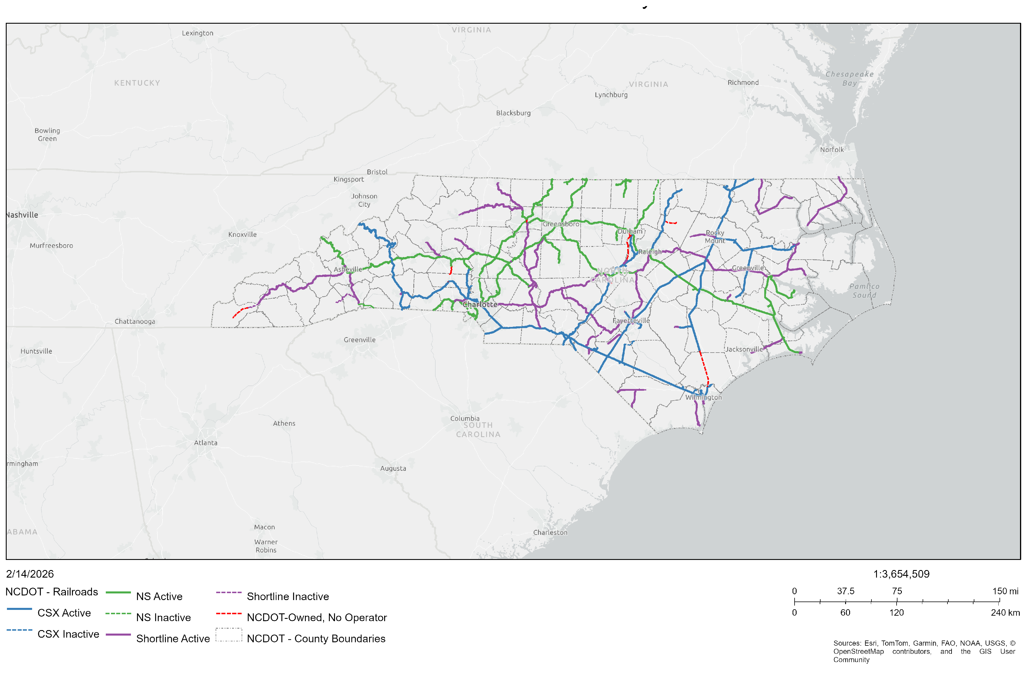
Figure 2.
Streamlined overview of the hot spot classification model.
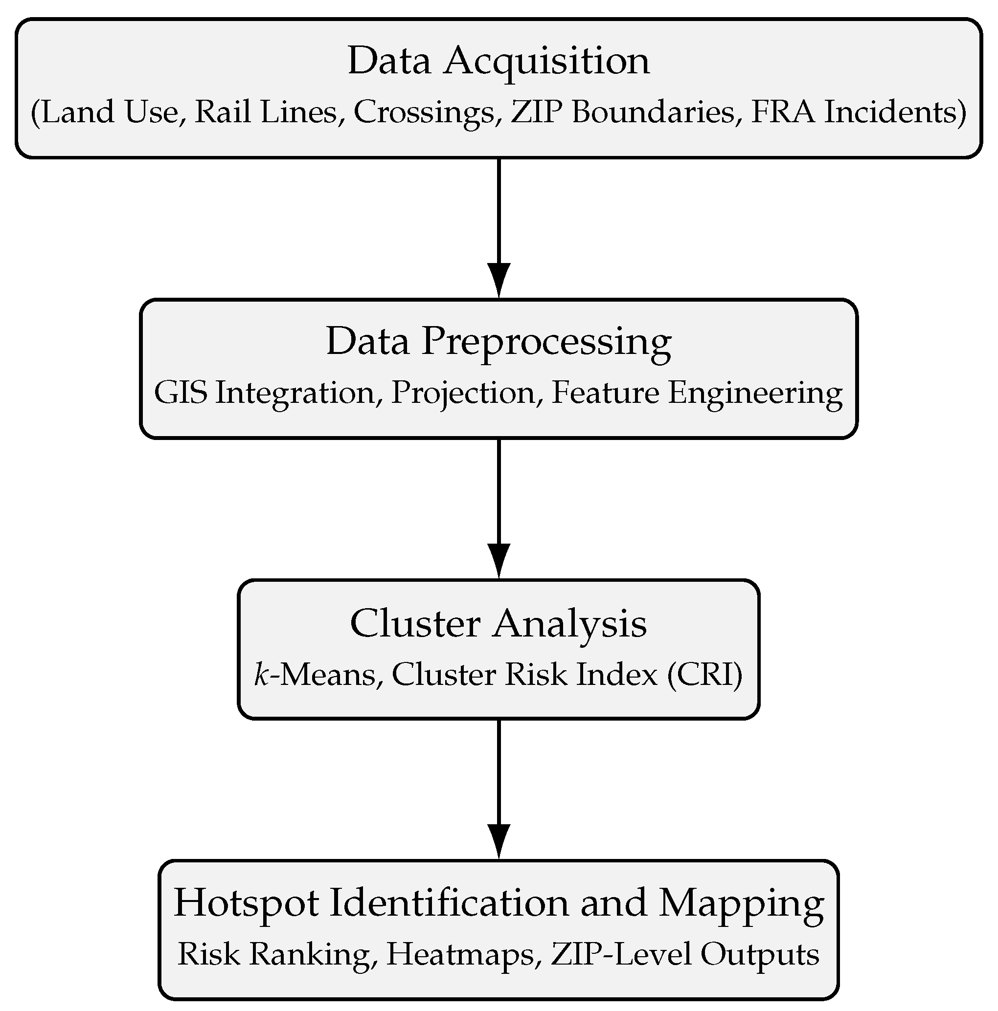
Figure 3.
Global Moran’s I across k.
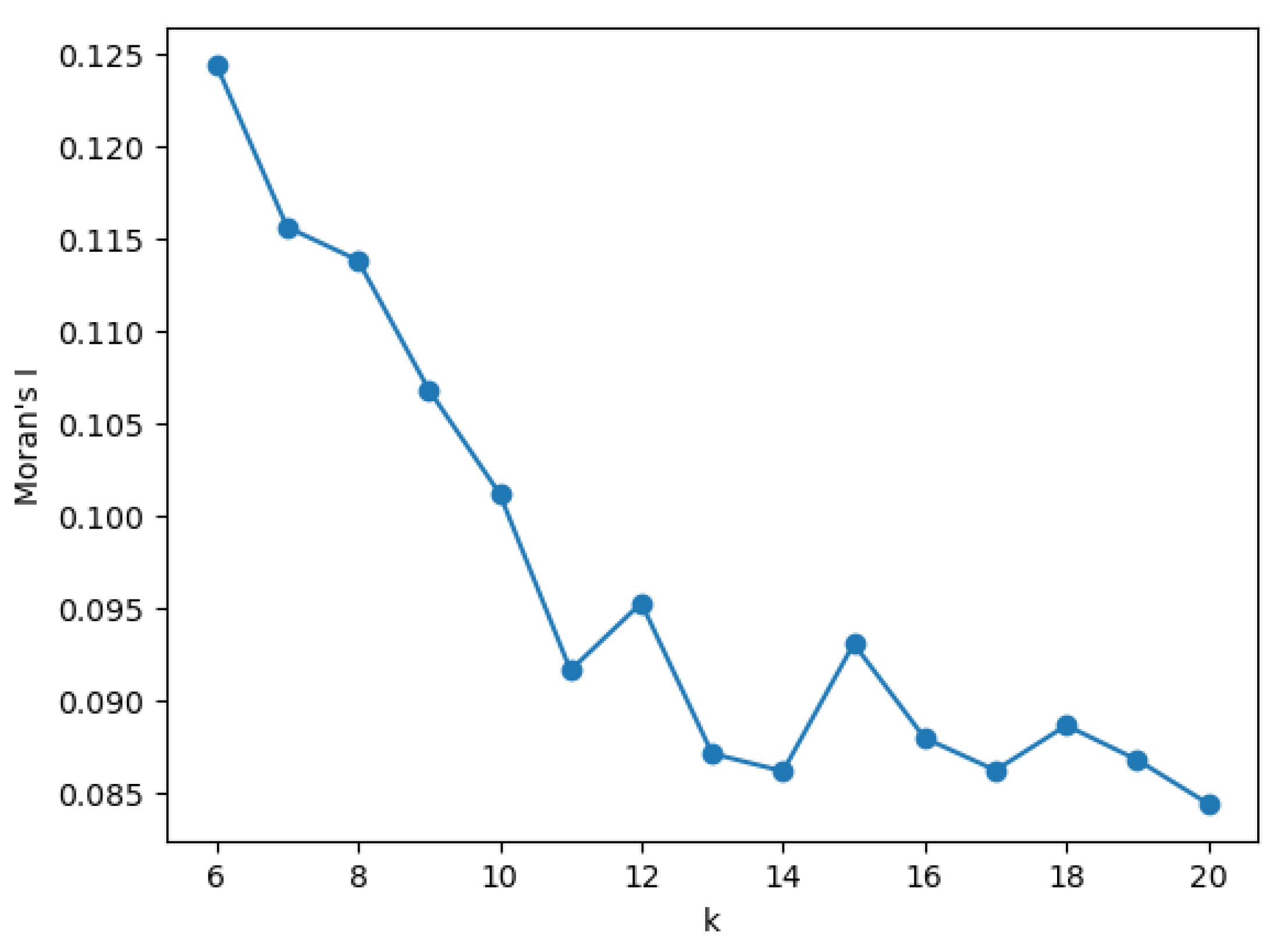
Figure 4.
Global Moran’s z-score across k.
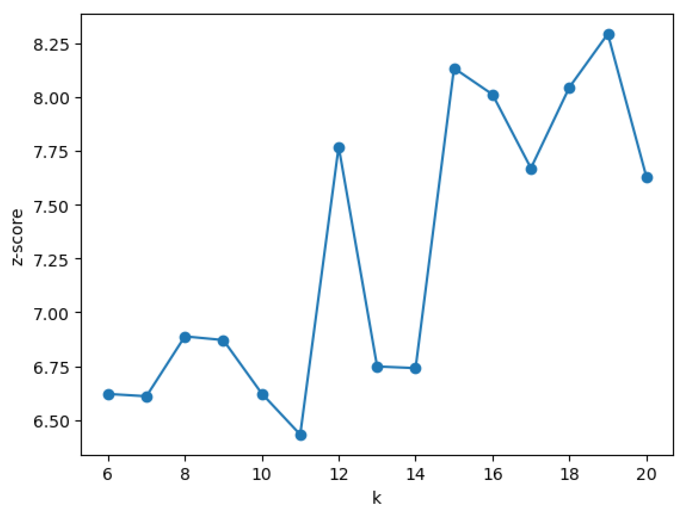
Figure 5.
LISA “volcano” plot of Local Moran’s I (x) versus (y). Orange points mark High–High (HH) clusters that remain significant after FDR correction (); labels indicate ZIP codes. The dashed horizontal line at corresponds to the nominal threshold.
Figure 5.
LISA “volcano” plot of Local Moran’s I (x) versus (y). Orange points mark High–High (HH) clusters that remain significant after FDR correction (); labels indicate ZIP codes. The dashed horizontal line at corresponds to the nominal threshold.
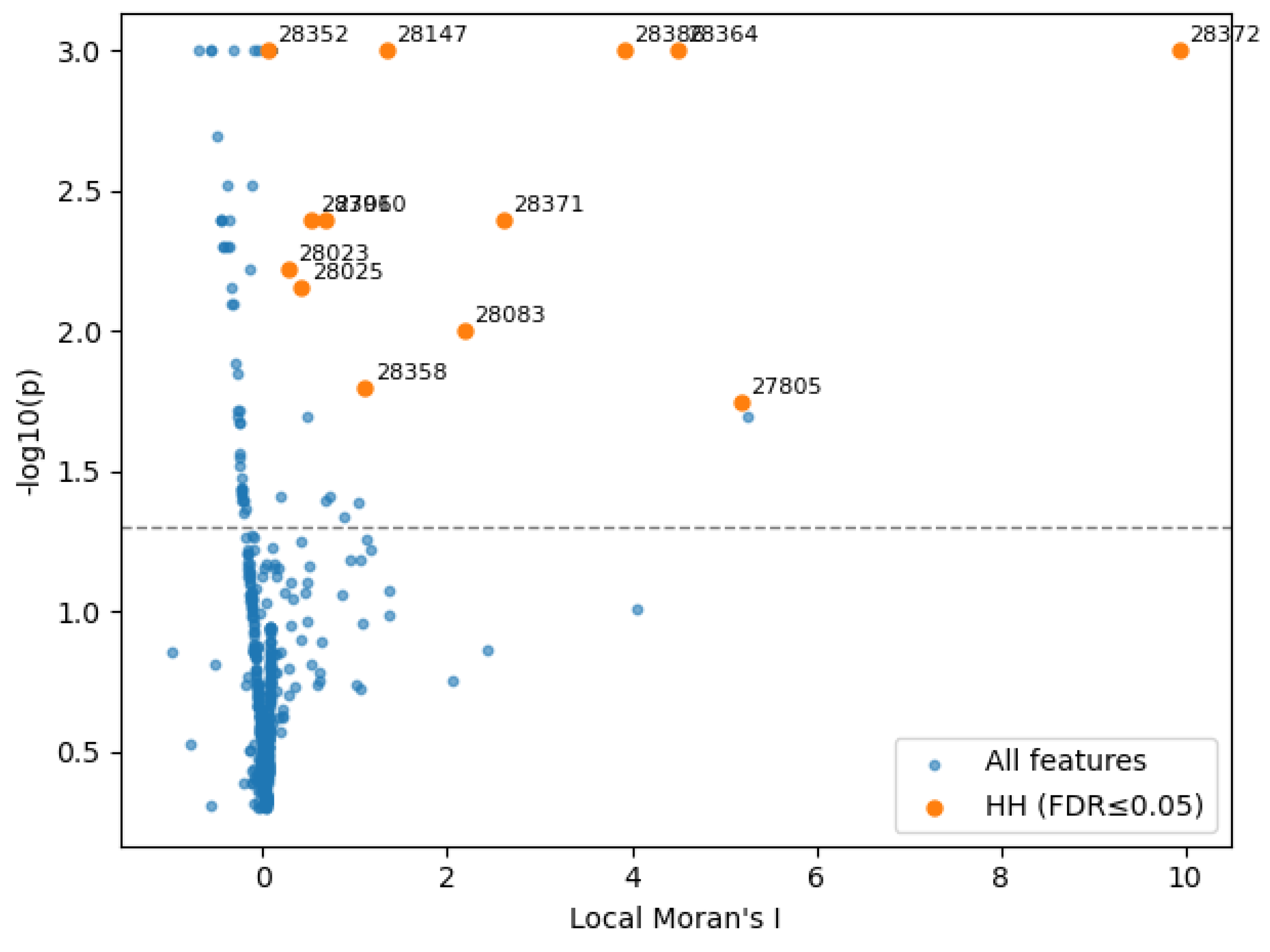
Figure 6.
Getis–Ord Gi* hot spots (feet band; 90–99%).
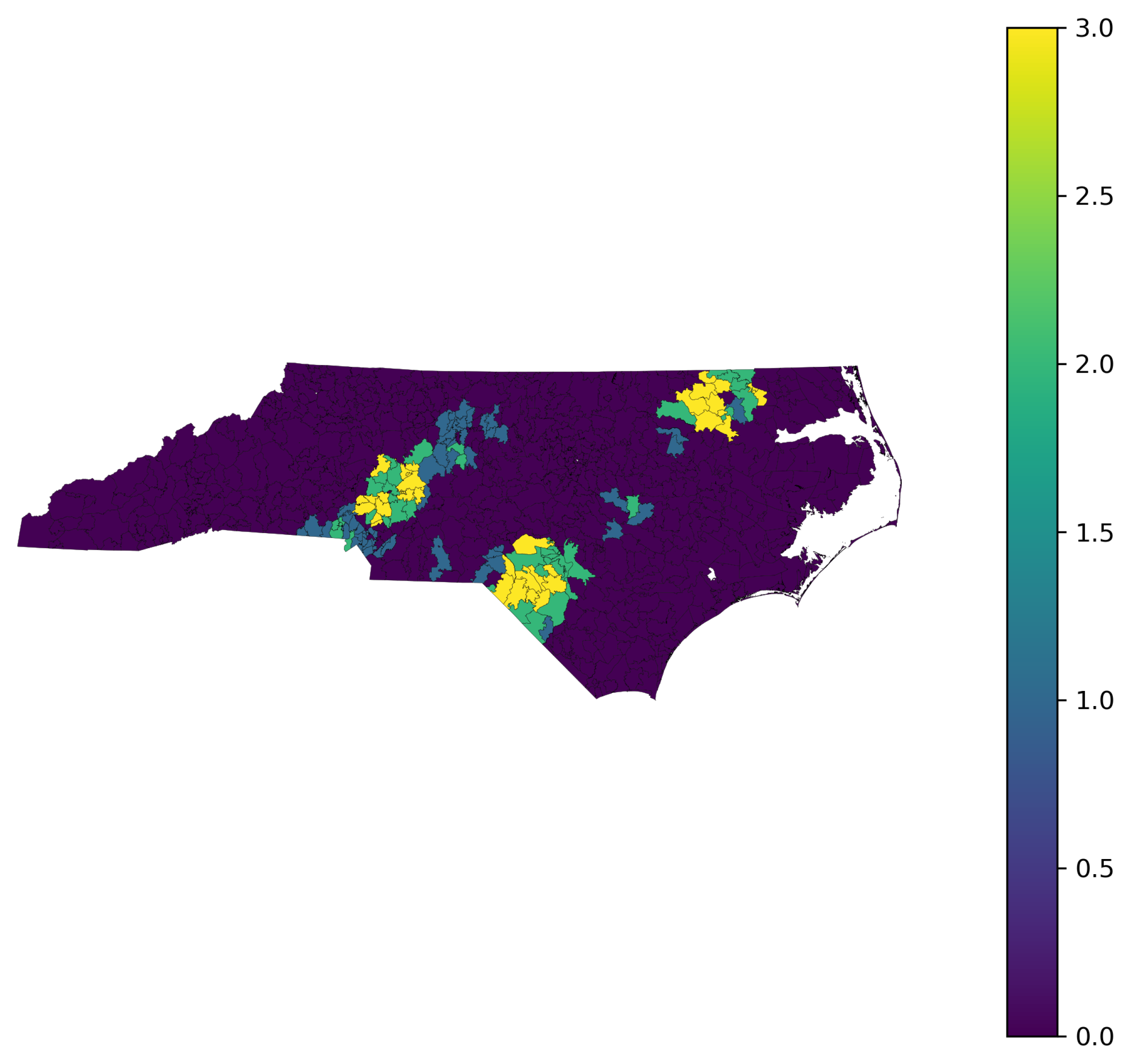
Figure 7.
LISA hot spots (k=10; FDR): High–High (HH).
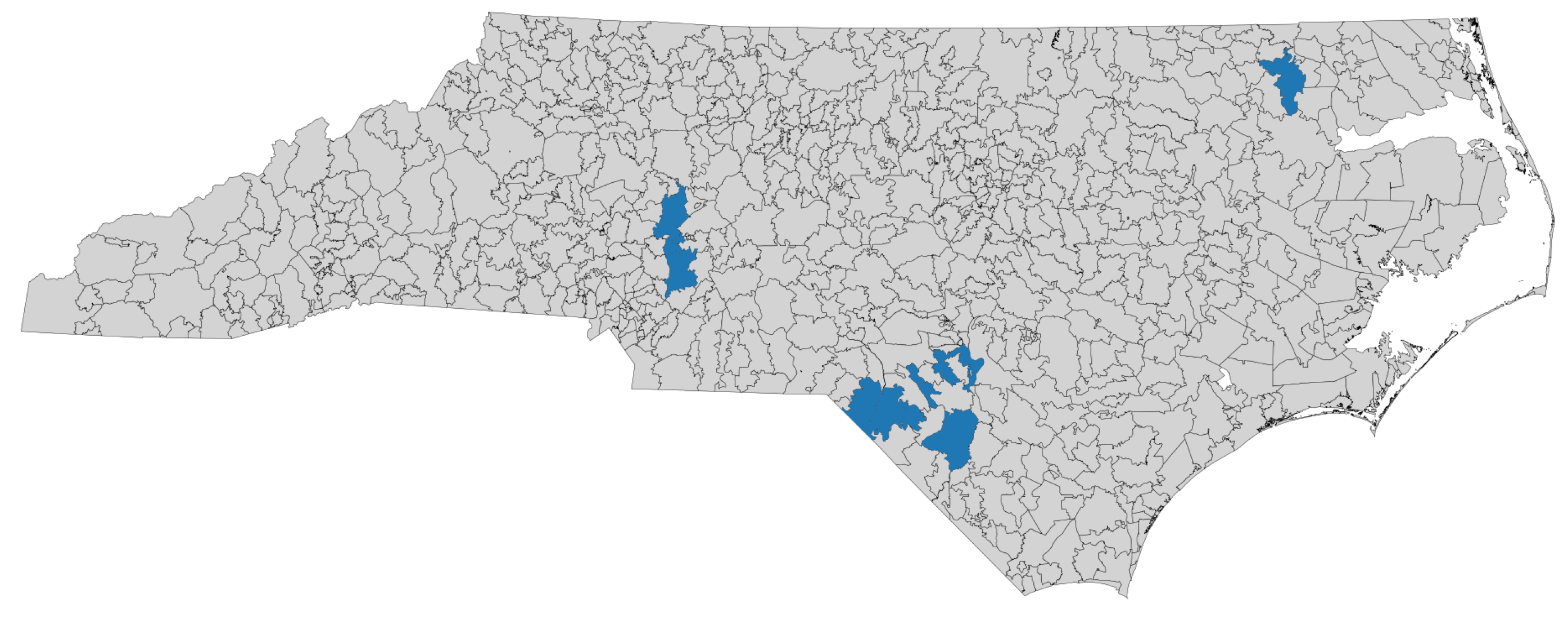
Figure 8.
Elbow method for selecting the optimal number of clusters in the k-means analysis.
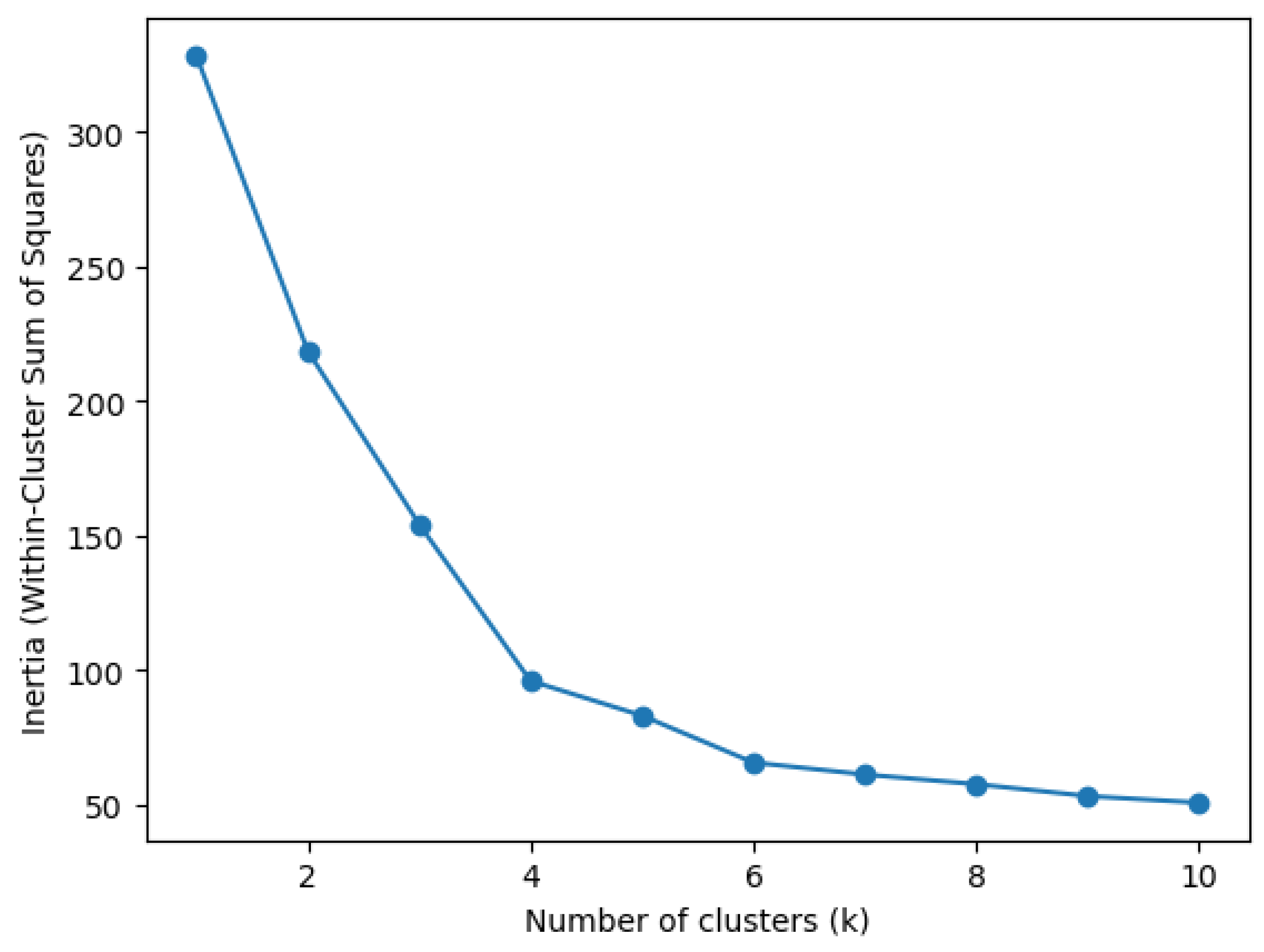
Figure 9.
Spatial distribution of the Cluster Risk Index (CRI) across ZIP codes in North Carolina.
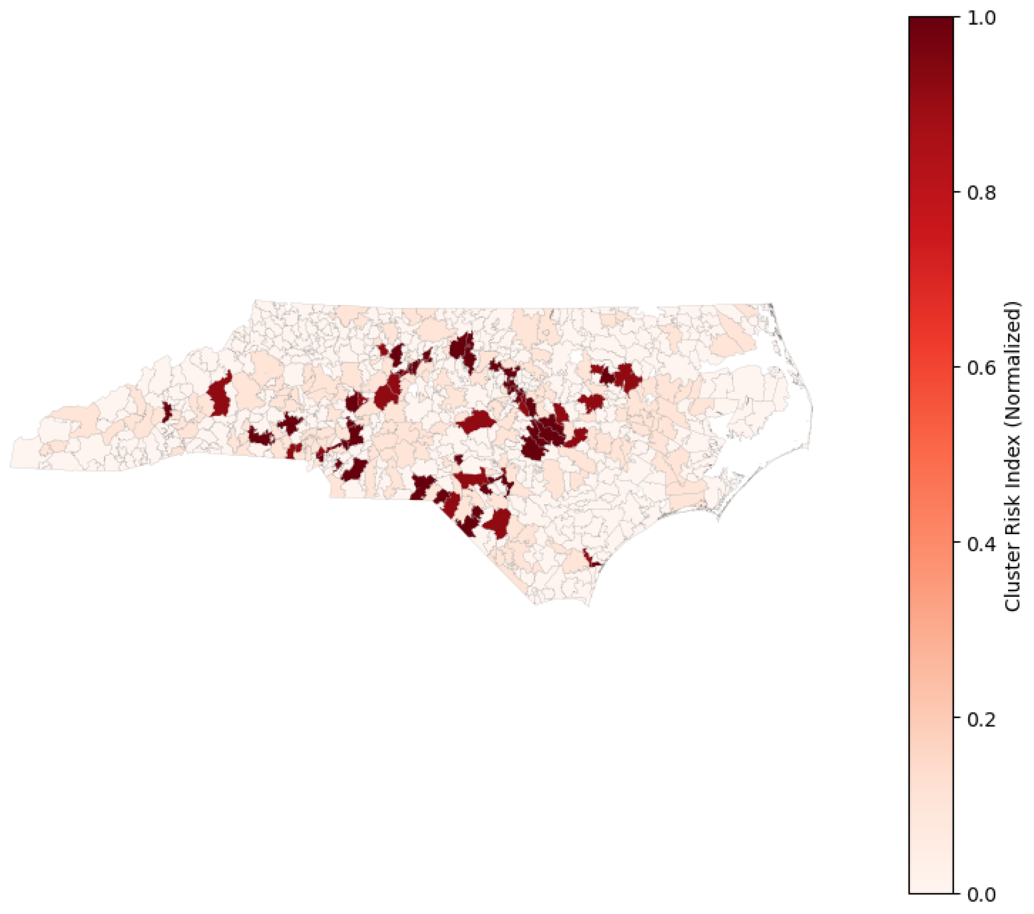

Table 1.
Descriptivr statistics of Zip code dataset.
| Variable | N valid | Mean | SD | Min | Median | Max |
|---|---|---|---|---|---|---|
| POPULATION | 766 | 14,054.405 | 16,632.172 | 0.000 | 6,837.500 | 85,514.000 |
| POP_SQMI | 766 | 604.747 | 1,561.992 | 0.002 | 125.785 | 22,950.000 |
| SQMI | 766 | 65.246 | 60.962 | 0.020 | 47.845 | 428.130 |
| Casualties | 766 | 0.663 | 1.903 | 0.000 | 0.000 | 17.000 |
| rate_per_10k | 763 | 0.374 | 1.253 | 0.000 | 0.000 | 14.577 |
Note. rate_per_10k excludes 3 ZIPs with zero/unknown population. Many ZIPs report zero casualties (median = 0), so rate distributions are right-skewed; permutation-based spatial statistics are therefore used throughout to avoid normality assumptions.
Table 2.
Descriptive Statistics of Railroad Crossing Purpose.
| Crossing Purpose | Count | Percentage (%) |
|---|---|---|
| Highway | 4,796 | 98.74 |
| Pathway, Pedestrian | 57 | 1.17 |
| Station, Pedestrian | 4 | 0.08 |
| Total | 4,857 | 100.00 |
Table 3.
Sample ZIP-Level Prediction Dataset.
| ZIP | Pop. | Pop./ sq. mi |
Area | Rail | Crossings | Casualties | Residential | Commercial | Industrial | Agricultural/ Rural |
Other land use |
|---|---|---|---|---|---|---|---|---|---|---|---|
| 27101 | 32,450 | 2,150.4 | 15.09 | 18.25 | 22 | 6 | 0.32 | 0.28 | 0.21 | 0.12 | 0.07 |
| 27514 | 24,890 | 1,480.6 | 16.81 | 9.40 | 11 | 2 | 0.41 | 0.24 | 0.12 | 0.18 | 0.05 |
| 28301 | 18,120 | 890.3 | 20.35 | 6.75 | 8 | 1 | 0.27 | 0.19 | 0.16 | 0.33 | 0.05 |
| 27896 | 6,540 | 95.2 | 68.68 | 0.00 | 1 | 0 | 0.05 | 0.02 | 0.01 | 0.90 | 0.02 |
| 28403 | 12,430 | 610.7 | 20.36 | 2.10 | 4 | 0 | 0.18 | 0.11 | 0.07 | 0.58 | 0.06 |
Note. Pop. = Population; Area = square miles; Rail = rail miles within ZIP. Land-use variables are proportional coverages that sum to 1.00.
Table 4.
Moran’s I values across different k-neighbors.
| k | Moran I | z score | p-value |
|---|---|---|---|
| 6 | 0.124407 | 6.536211 | 0.001 |
| 7 | 0.115609 | 6.603078 | 0.001 |
| 8 | 0.113817 | 7.049733 | 0.001 |
| 9 | 0.106806 | 6.886261 | 0.001 |
| 10 | 0.101180 | 7.174451 | 0.001 |
| 11 | 0.091619 | 6.359131 | 0.001 |
| 12 | 0.095258 | 7.209565 | 0.001 |
| 13 | 0.087108 | 6.742585 | 0.001 |
| 14 | 0.086150 | 6.862160 | 0.001 |
| 15 | 0.093052 | 8.265287 | 0.001 |
| 16 | 0.087048 | 7.556754 | 0.001 |
| 17 | 0.086203 | 7.652760 | 0.001 |
| 18 | 0.088630 | 8.241578 | 0.001 |
| 19 | 0.086769 | 8.115465 | 0.001 |
| 20 | 0.084399 | 8.533200 | 0.001 |
Table 5.
Top ZIPs with localized casualty clustering.
| ZIP Code | Casualties | Casualty rate per 10K population | City | County |
|---|---|---|---|---|
| 28372 | 10 | 7.3180 | Pembroke | Robeson |
| 28386 | 2 | 3.4819 | Shannon | Robeson |
| 28371 | 2 | 2.8413 | Parkton | Robeson |
| 28364 | 3 | 2.5482 | Maxton | Robeson |
| 28147 | 4 | 1.4793 | Salisbury | Rowan |
| 27910 | 3 | 0.9696 | Ahoskie | Hertford |
| 28306 | 4 | 0.8951 | Fayetteville | Cumberland |
| 28025 | 5 | 0.8183 | Concord | Cabarrus |
| 28023 | 1 | 0.6660 | China Grove | Rowan |
| 28352 | 1 | 0.4089 | Laurinburg | Scotland |
Table 6.
K-Means Cluster Centroids Based on Rail Exposure, Population Density, and Land-Use Composition.
Table 6.
K-Means Cluster Centroids Based on Rail Exposure, Population Density, and Land-Use Composition.
| Cluster | Rail Miles | Crossings | POPU_SQMI | Pct_Res. | Pct_Comm. | Pct_Ind. | Pct_Agric. |
|---|---|---|---|---|---|---|---|
| 0 | 0.98 | 1.82 | 547.62 | 0.196 | 0.222 | 0.140 | 0.371 |
| 1 | 5.78 | 15.46 | 436.26 | 0.217 | 0.174 | 0.292 | 0.256 |
| 2 | 31.58 | 39.71 | 1104.54 | 0.158 | 0.210 | 0.341 | 0.204 |
| 3 | 17.44 | 11.85 | 1301.47 | 0.282 | 0.233 | 0.265 | 0.190 |
Table 7.
Hotspot Probability, Relative Risk, and Cluster Risk Index (CRI) by ZIP Code Cluster
| Cluster | ZIPs | Hotspots | Hotspot Prob. | Rel. Risk | CRI | |||
|---|---|---|---|---|---|---|---|---|
| 0 | 519 | 39 | 0.075 | 0.055 | 0.101 | 0.128 | 0.010 | 0.000 |
| 1 | 158 | 51 | 0.323 | 0.255 | 0.399 | 0.548 | 0.177 | 0.099 |
| 2 | 24 | 23 | 0.958 | 0.798 | 0.993 | 1.627 | 1.559 | 0.918 |
| 3 | 41 | 41 | 1.000 | 0.914 | 1.000 | 1.698 | 1.698 | 1.000 |
Disclaimer/Publisher’s Note: The statements, opinions and data contained in all publications are solely those of the individual author(s) and contributor(s) and not of MDPI and/or the editor(s). MDPI and/or the editor(s) disclaim responsibility for any injury to people or property resulting from any ideas, methods, instructions or products referred to in the content. |
© 2026 by the authors. Licensee MDPI, Basel, Switzerland. This article is an open access article distributed under the terms and conditions of the Creative Commons Attribution (CC BY) license (http://creativecommons.org/licenses/by/4.0/).
Copyright: This open access article is published under a Creative Commons CC BY 4.0 license, which permit the free download, distribution, and reuse, provided that the author and preprint are cited in any reuse.


