Submitted:
18 February 2026
Posted:
19 February 2026
You are already at the latest version
Abstract
To investigate the long-term effects of climate change on biological communities, our primary aim was to identify the most reliable indicators among available biodiversity, dominance, and evenness indices. We examined three distinct response types to climate change, represented by three taxonomic groups: Aculeata (Hymenoptera), Syrphidae (Diptera), and nocturnal macrolepidoptera (Lepidoptera). Using faunistic datasets derived from our own 3–5 decades of field surveys, we calculated 12 key indices with the vegan package in R 4.2.1. The robustness of these indices was assessed through 1000-fold bootstrap simulations and pairwise correlation analyses. Our results revealed that the Gini–Simpson, Simpson diversity, McIntosh diversity, and McIntosh evenness indices consistently demonstrated high temporal stability and strong correlations across all three climate response types. Therefore, we recommend these indices as primary climate indicators. In contrast, Chao1 estimates, Margalef Index, Menhinick Index, and the Shannon–Wiener diversity index are suitable only for analyzing specific response patterns. Meanwhile, the Berger–Parker, Buzas–Gibson indices, and Hill numbers showed high variability or limited ecological responsiveness, making them unreliable for tracking climate change impacts. Our findings underscore that selecting biodiversity indices must be tailored to the research question and the characteristics of the ecosystem in order to ensure valid and informative ecological analysis.
Keywords:
climate change
; ecology
; biodiversity
; dominance and evenness indices
; insects
; Hymenoptera (Aculeata)
; Diptera (hoverflies)
; Lepidoptera (moths)
; terrestrial biomes
; temperate zone
1. Introduction
The quantification of ecological diversity and species richness—together with their spatial patterns and temporal dynamics—emerged as a pressing scientific priority as early as the mid 20th century [1,2]. Over the past 80 years, a wide array of indices has been mathematically formalized [3,4,5,6,7,8]. Their functionality has also diversified, leading to the classification of indices into three principal categories: Richness indices, which quantify species richness or its estimation (e.g., Chao1, Margalef, Menhinick); Evenness and dominance indices, which assess the uniformity and dominance structure of species distributions (e.g., Berger–Parker dominance, Buzas–Gibson, McIntosh evenness, Simpson diversity, Gini–Simpson index); Composite indices, which integrate both species number and distribution (e.g., Shannon–Wiener index, Hill numbers, McIntosh diversity index).
The proliferation of statistical methods has produced contradictions among results, a common outcome in quantitative ecology. This issue has only recently been emphasized by Kitikidou et al. [9]. From this point onward, it becomes the responsibility of contemporary ecological science to define and delimit the role and relevance of these tools. Only by doing so can we avoid constructing a distorted representation of ecological reality. Motivated by this work titled Using Biodiversity Indices Effectively: Considerations for Forest Management [9]., we examine—through the statistical approaches presented herein—the suitability of the most commonly applied biodiversity, evenness, and dominance indices in the context of global climate change.
Building on the work of Kitikidou et al. [9], our central hypothesis is that the applicability of individual indices is fundamentally shaped by the specific characteristics of the various types of ecological investigations in which they are employed. Accordingly, our objective is to determine which biodiversity indices yield robust and interpretable information when applied to time series influenced by climate change, and which indices are less suitable for such analyses.
The evaluation of these twelve indices appears in numerous studies, yet most of these publications address only their spatial applicability and limitations [10,11,12,13,14,15,16,17]. Other authors do not examine the applicability of classical indices to time series or to the temporal analysis of climate change; instead, they introduce new or previously seldom-used metrics and indicators [18,19,20]. Only a small number of scientific publications investigate the temporal applicability of classical biodiversity indices. Guan et al. (2025) [21] consider the Shannon diversity index (SHDI) suitable for assessing the impacts of climate change, although they apply it to spatial patterns, specifically to quantify climate heterogeneity along elevation gradients. Twaróg (2025) [22] confirms that Shannon entropy is appropriate for analyzing temporal dimensions of climate change. Huang and Fu (2023) [23] find both the Shannon and Simpson indices suitable for examining the temporal effects of climate change and apply them in their analysis of α-diversity dynamics in Tibetan grasslands. In assessing environmental health, Supriatna [24] highlights the Shannon and Simpson indices as particularly effective: “Both indexes are more reflective in nature and can predict the environment health.”. Similarly, the monograph by Nicholas Gotelli and Anne Chao [25] provides a critical overview of numerous indices—including Simpson, Gini–Simpson, Sørensen, Jaccard, Morisita–Horn, Horn index, Hill numbers, and the Chao–Jaccard and Chao–Sørensen estimators—outlining their general limitations. Despite their widespread use across tens of thousands of publications, rigorous methodological scrutiny of these indices has remained scarce—emerging only in the past decade and even then in just a few studies.
The study area encompasses the territory of Hungary, a region that exemplifies the climatic characteristics of Central Europe, particularly in low-elevation landscapes (100–1,000 m). Across the study period (1970–2024), a pronounced warming trend is evident: raw observations indicate an increase in mean annual temperature of approximately +3.1 °C.
Parallel to this warming, several key climatic indicators have shifted markedly. The number of frost days has declined substantially, decreasing from roughly 105 to 65 days per year. In contrast, the frequency of hot days and heatwaves has risen sharply: hot days increased from about 10 days per year in the early decades to nearly 60 days by 2024, while heatwave days—once limited to 0–4 days annually—have regularly reached several tens of days per year since the 2000s. Annual precipitation totals exhibit a downward tendency (from 698 mm to 526 mm), although interannual variability remains considerable. Recent years also show elevated solar radiation and insolation levels, consistent with observed changes in cloud cover and broader atmospheric dynamics [26]. These climatic shifts—fewer frost days, more frequent and intense heat events, and increasingly common heatwaves—carry direct and far-reaching ecological and societal implications.
2. Materials and Methods
2.1. Hymenoptera, Diptera
Our results are derived from faunistic surveys conducted systematically across the past five decades in multiple regions of the Carpathian (Pannonian) Basin. The research is grounded in standardized, continuous sampling efforts extending over four to five decades, beginning in the 1970s and 1980s. For Aculeata, a total of 1,318 sampling sites were surveyed, while Syrphidae were sampled at 2,086 sites, with 30–35 field days per year depending on prevailing weather conditions.
The reliability and internal consistency of the dataset are strengthened by the fact that sampling was performed by the same individual collectors over the entire study period, using unchanged methodologies. Hymenoptera were collected by Zsolt Józan exclusively through sweep-netting, whereas Syrphidae were collected by Sándor Tóth using sweep-netting supplemented once annually by a Malaise trap deployed at varying locations. These methodological details are described comprehensively in Tóth’s 1994 publication [27]. The long-term continuity of these surveys reflects the lifelong commitment of the individual researchers involved.
As a consequence, factors that typically introduce variability into sweep-net sampling—such as net dimensions, sweep arc, or the collector’s arm length—remained effectively constant over the decades. This exceptional methodological consistency provides a rare degree of temporal comparability, enhancing the robustness of the resulting ecological time series. All aggregation intervals of these data-series are of equal length. The full years of collecting activity—which cover most of the active working period of the collectors Zsolt Józan and Sándor Tóth—were divided into equal 5- or 6-year periods. Years with low collecting intensity due to illness, relocation, or other personal circumstances were excluded. During this period, they collected roughly 160,000 Aculeata specimens and 117,000 hoverflies.
The collected material is stored in part at the Natural History Museum in Zirc, the Rippl-Rónai Museum in Kaposvár, and the Hungarian Natural History Museum. The primary method was sweep netting, with Diptera sampling supplemented by one annual Malaise trap session. While data on nocturnal moths remain unpublished, Hymenoptera and Diptera data have been partially published [28,29,30,31,32].
2.2. Nocturnal Macrolepidoptera
Species richness and abundance of nocturnal moths were analyzed using light-trap data derived from long-term faunistic surveys conducted across the Carpathian Basin. The study relied primarily on the Hungarian Forestry Light Trap Network, which provides extensive nationwide coverage and represents one of the most consistent sources of standardized Lepidoptera monitoring data in the region. Species identification was carried out by specialists including Csaba Szabóky, Csaba Gáspár, Lajos Kovács, Katalin Leskó, Levente Ábrahám, Ákos Uherkovich, Zoltán Varga, and Péter Schmidt, among others.
Wherever possible, individual light-trap sites were monitored continuously for several decades. In other cases, the same regions—such as Zselic and Ormánság—were resurveyed after intervals of 40 to 50 years [33,34]. Changes in light-trap technology were also taken into account. Since 2014, UV LED light traps have replaced the 20 W black-light UV lamps that were standard between 1990 and 2010. In addition, several Jermy-type traps within the Forestry Light Trap Network have operated with 125 W mercury-vapor lamps for more than 30–40 years, functioning daily from early March through late December [35]. Because these light sources differ in their selectivity and capture efficiency, their effects were explicitly considered in the trend analyses [36,37].
Previous studies have already examined diversity patterns and biotic homogenization using forestry light-trap datasets [38]. For the present analysis, only those data series that included at least six months of uninterrupted daily sampling—typically spanning April to October—were retained. Traps operated continuously throughout these periods. Shorter or incomplete time series were excluded to ensure comparability and analytical robustness.
2.3. Statistical Considerations in Ecological and Meteorological Data Collection
2.3.1. Data Preparation and Processing
In taxa with exceptionally large numbers of sampling sites—such as Aculeata and hoverflies (Syrphidae), with 1,300–2,100 collection points—data from a single year, typically representing roughly 35 sampling days, provide only limited insight into regional ecological conditions. When observations are aggregated over a five-year period (approximately 175 sampling days), the resulting dataset offers a far more reliable and representative picture of the ecological state of a given region during that interval.
Trend analysis is a fundamental ecological tool [39,40,41], frequently applicable with temporal aggregation to reveal underlying trajectories. Given the substantial natural year-to-year variability characteristic of ecological systems, multi-year aggregation is not merely justified but essential. It enables the detection of long-term trends and structural patterns that would otherwise be obscured by short-term fluctuations or stochastic noise. The principal advantages of temporal aggregation include the reduction of random variation and periodic shifts, mitigation of biases associated with field conditions or observer fatigue, and diminished influence of climatic anomalies. Although aggregation inevitably reduces temporal granularity and may appear to decrease sample size, it substantially enhances the clarity and interpretability of trend analyses. When annual datasets exhibit high variance, long-term grouping smooths inconsistencies and reveals genuine ecological trajectories [36,37].
In other cases, the sampling methodology of the focal taxon—such as nocturnal moths—does not permit such aggregation. Nevertheless, even with a limited number of sampling sites (light traps), it is possible to obtain exceptionally large sample sizes, often approaching 350,000 individuals. Under these circumstances, individual traps can be analyzed independently. Trap locations were selected to ensure coverage of diverse landscape units and biotopes, thereby maximizing the ecological representativeness of the study area.
Climatic parameters—including mean temperature, total precipitation, number of precipitation days, number of frost days, number of hot days, and number of heatwave-affected days—were obtained from the Hungarian Central Statistical Office [26].
2.3.2. Index Calculation
All dominance and diversity indices were calculated in R version 4.2.1 [40] using the vegan [43] and BiodiversityR [44] packages, supplemented by simple custom R scripts. Specifically, we used the functions diversity and estimateR in vegan with default settings. In the constructed species matrix, zeros denoted the absence of a given species. For detailed calculation methods and formulas of individual indices, see in Kitikidou et al. [9].
2.3.3. Correlation with Environmental Variables
Following the calculation of each index, we quantified the strength of their relationships with the measured components of climate change by determining both the coefficients of determination and the corresponding correlation coefficients. The components and their notations are: R2T – coefficient of determination for temperature; rT – correlation coefficient for temperature; R2M – coefficient of determination for precipitation amount; rM – correlation coefficient for precipitation amount; R2P – coefficient of determination for number of precipitation days; rP – correlation coefficient for number of precipitation days; R2F – coefficient of determination for number of frost days; rF – correlation coefficient for number of frost days; R2H – coefficient of determination for number of hot days; rH – correlation coefficient for number of hot days; R2W – coefficient of determination for number of heatwave days; rW – correlation coefficient for number of heatwave days. R2 indicates the proportion of variance explained by the climatic factor, and r indicates the direction and strength of the relationship.
2.3.4. Robustness and Pairwise Analysis
In the next step, we subjected all indices to bootstrap and pairwise analyses [45,46,47,48,49]. The bootstrap procedure was used to evaluate the robustness of each index. In this context, robustness refers to the stability and reliability of the temporal trajectories of the indices even when the underlying data contain minor deviations, statistical noise, or distributional irregularities. Bootstrap resampling was performed with 1,000 iterations, and a robustness threshold of CV < 10% was applied, as values below this level are generally considered minimally sensitive to random sampling bias.
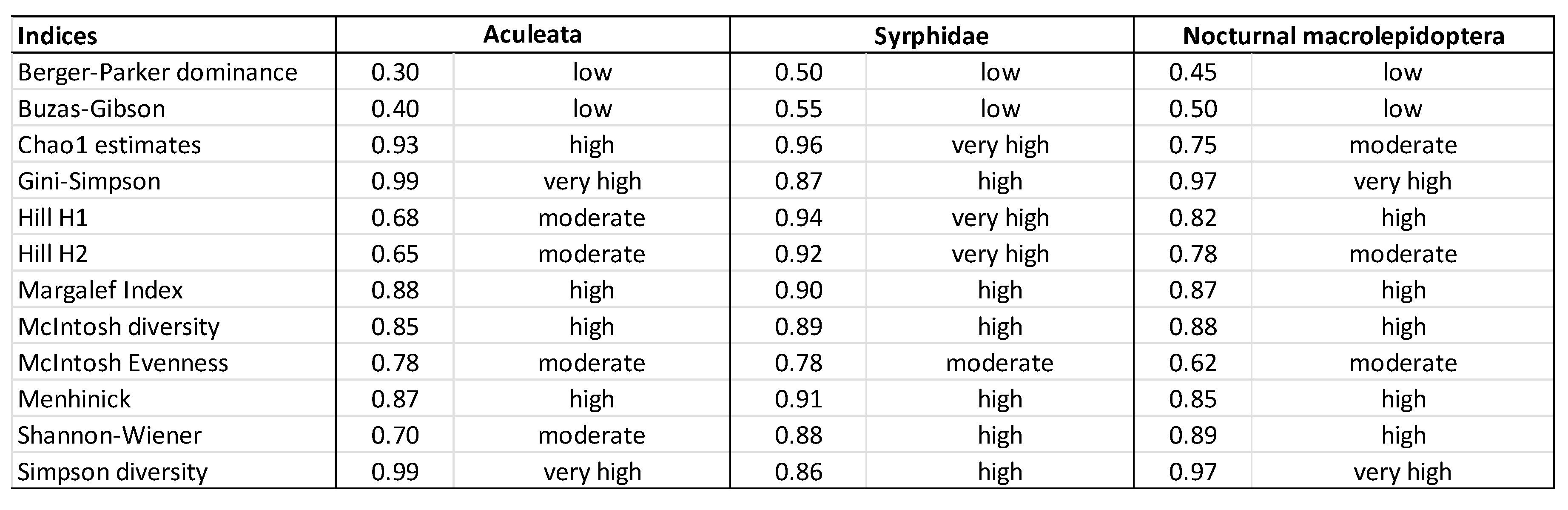
Subsequently, the index time series were examined using pairwise analysis following the methodology of Kitikidou et al. [9]. Pairwise analysis identifies statistical and correlational relationships among the time series (i.e., the temporal sequences of the indices), revealing the degree to which their dynamics converge or diverge over time. The resulting Mean Pairwise r value represents the average of all pairwise Pearson correlation coefficients across the index time series. High Mean Pairwise r values (approaching 1) indicate that the indices exhibit strongly similar temporal patterns and are positively correlated, whereas values near 0 reflect the absence of meaningful relationships. An index that consistently yields high Mean Pairwise r values is likely to measure the same underlying component of diversity or species richness in a reliable manner.
An index is considered suitable for describing and analyzing ecological responses to climate change (and other long-term processes) if it aligns with directly measured changes in individual abundance and species richness, provides additional explanatory value beyond these basic metrics, demonstrates statistical robustness, and accurately reflects the ecological response of the focal taxon to environmental change. Furthermore, it must not exhibit contradictions in the direction or strength of correlations during pairwise analysis.
For nocturnal macrolepidoptera, identical light sources have been used since 2019. From that year onward, all indices were re-evaluated using both bootstrap and pairwise analyses. Finally, we assess the applicability of the various indices in capturing three distinct insect responses to climate change. The applied methods are summarized in Table 1.
3. Results
3.1. Assessment of Three Types of Responses to Climate Change
3.1.1. Assesment of the Ecological Response of Thermophilic Groups for Climate Change
The first response is the increase in abundance of thermophilic groups in line with rising annual average temperatures (Figure 1). This group is represented here by the Aculeata (bees, wasps, cuckoo wasps, sphecoid wasps, spider wasps etc.). While some species within this group are hylophilous, the term xerothermic best characterizes the group as a whole.
It is evident (see Supplementary Material) that in this response type, community diversity increased, dominance declined, and species composition became more evenly distributed. Both individual abundance and species richness rose in parallel with increasing temperatures. Most diversity indices showed strong positive correlations with temperature and the number of heatwave days (rT = 0.61–0.64; rW = 0.79–0.80). For example: Gini–Simpson: rT = 0.63, rW = 0.80; Hill H2: rT = 0.64, rW = 0.80; Simpson: rT = 0.61. Dominance (Berger–Parker) exhibited a strong negative correlation with temperature and heatwaves (rT = −0.67, rW = −0.81), which is expected: as diversity increases, dominance decreases, meaning that formerly common species exert less control over community structure.
The number of frost days showed a negative correlation with nearly all indices, indicating that more frost days are associated with lower diversity. Precipitation amount and the number of precipitation days displayed weaker but generally positive relationships (typically r = 0.1–0.5). The strongest correlations were observed for Chao1 (rM = 0.74) and the Margalef index (rM = 0.79). Although precipitation tends to increase species counts, its effect is weaker than that of temperature. Most diversity indices proved robust for this ecological response type (Supplementary Material), and pairwise analysis revealed strong, positively aligned correlations for Chao1 estimates, the Gini–Simpson index, the Margalef index, McIntosh diversity, Menhinick, and Simpson diversity.
3.1.2. Assessment of the Ecological Response of Hygrophilous Groups for Climate Change
The second type of climate-change response is best exemplified by hoverflies (Syrphidae) (Figure 2, Supplementary Material), whose populations have undergone severe global declines [36,50]. This decline shows a strong association with rising temperatures [37]. The indices and the summary of their bootstrap performance are provided in the Supplementary Material. For most indices, rT values fall between 0.82 and 0.93, indicating exceptionally strong correlations—the strongest temperature effect observed among all examined groups. However, the positive correlations for most indices can be misleading and appear contradictory to the observed outcomes. The data show that, despite a sharp decline in individual abundance closely linked to increasing annual mean temperatures, overall community diversity increased. Warmer periods were characterized by fewer individuals but a more balanced species composition.
Precipitation amount (rM) exerted a weak and inconsistent influence, suggesting that hoverfly diversity is not strongly dependent on rainfall. The number of precipitation days (rP) showed a weak negative effect, likely reflecting reduced flight activity during wet conditions. Frost days had a moderately strong negative effect. Based on diversity indices, Syrphidae appeared to be thermophilic, since temperature and heatwave days showed strong positive correlations with diversity. However, the abundance data tell a very different story, and this is a crucial distinction. What does abundance show? Abundance rT = −0.81563, rH = −0.8801, and rW = −0.8516. These are very strong negative correlations. So why does diversity increase? This is the key point.
Extreme warm events (H, W) play a key role, particularly for hoverflies, where heat and heatwaves account for much of the variation in diversity and dominance; this suggests that future warming and more frequent heat extremes could drive rapid and pronounced community reorganization. For Aculeate (most wasps and bees), precipitation and frost frequency are important: changes in rainfall amount and rainy-day frequency are likely to directly affect species richness and Chao1 estimates, while frost frequency strongly structures dominance patterns. Divergent responses in abundance, diversity and evenness imply that climate change will alter not only species counts but also dominance hierarchies and community evenness, with potential consequences for ecosystem functions mediated by these insect assemblages.
Hoverfly communities show stronger, more direct negative responses to mean temperature increases and heat extremes (high R2 and r values), whereas Aculeate responses are positive and more complex, with precipitation and frost days also exerting major influence. These differences are ecologically significant because they indicate that warming and altered precipitation regimes will reshape the two groups’ community structure and functional roles in different directions and magnitudes.
The relative stability in species richness suggests that no new species emerged, but rather that the proportions of existing species shifted. In this response type, the Chao1, Gini–Simpson, Margalef, McIntosh diversity, and Simpson diversity indices proved to be robust indicators (see Supplement mateiral). These indices effectively reflect ecological trends, whereas the remaining indices appear to be strongly influenced by sampling variability.
3.1.3. Assessment of the Ecological Response of Groups Exhibiting Low Sensitivity to Climate Change
The third type of response to climate change is represented by nocturnal moths (Figure 3; Supplementary Material). Their population density appears broadly stable and does not exhibit a clear directional response to temperature trends. The number of species captured per trap shows only a weak linear trend (R2 = 0.21), accompanied by a moderately strong negative correlation with rising annual mean temperatures (R2ₜ = 0.368, rₜ = –0.5539). The pattern observed in nocturnal Lepidoptera differs markedly from that of Aculeata and hoverflies. Moth communities are considerably less responsive to climatic variables, and the correlations are generally weaker.
For most indices, the relationship with temperature (rT) is weak to moderately negative (−0.587 to −0.3686), indicating that species richness and diversity tend to decline in warmer years. The effect of precipitation is minimal across nearly all indices (rM between −0.17 and +0.11). The number of precipitation days (rP) shows weak positive correlations (+0.1186 to +0.1346), suggesting that increased rainfall frequency may slightly enhance diversity, likely through stabilizing vegetation structure and microclimatic conditions. Frost days (rF) produce one of the stronger—though still moderate—patterns (+0.3594 to +0.5714). Hot days (rH) show a moderate negative relationship (−0.5189 to −0.3174), consistent with the sensitivity of many moth species to elevated temperatures. Heatwave days (rW) also exhibit moderately strong negative correlations (−0.3108 to −0.4764), indicating that heatwaves are particularly detrimental to nocturnal lepidopteran communities.
However, what is less apparent from the Supplementary Material is that dominant species have undergone near-complete turnover (see [37]). Moreover, the apparent stability in overall population size is largely attributable to the gradation cycles of certain species [37,51,52,53,54,55], which can mask underlying declines or shifts in community structure.
On average, communities have become species-poorer. Dominance levels are relatively even, consistent with previous observations [37], although 75% of dominant species have been replaced—a shift that diversity indices alone cannot captureThe indices found to be robust—Gini-Simpson Index, McIntosh Diversity, Shannon Diversity, and Simpson Diversity—exhibited exceptionally low coefficients of variation (CV < 10%), indicating stable values across bootstrap simulations. Most r and R2 values associated with indices for moths (nocturnal macrolepidoptera) are low (generally < 0.35) in contrast to the significantly stronger r and R2 observed for hoverflies and Aculeate Hymenoptera. For moths, there is no clear, strong positive or negative trend toward warming. Also, cold days and precipitation show moderate effects on some indices, but these effects are not consistent. Within this group, abundance and diversity are only weakly linked to the climatic variables examined; there is no pronounced inverse abundance–diversity pattern like the one observed between Aculeata and hoverflies. Overall, the data for nocturnal macrolepidoptera show substantially weaker univariate, linear climate explanatory power than those for hoverflies and, to some extent, Aculeate (Hymenoptera). This suggests that moth communities are shaped by more complex, multi factor mechanisms and that conventional forecasts based solely on temperature or precipitation are likely to be less reliable for them.
Pairwise analysis yielded high reliability (Mean Pairwise r ≥ 0.90) only for the Simpson Diversity and Gini-Simpson indices. The other two robust indices—Shannon-Wiener and McIntosh Diversity—also performed well, with reliability scores of 0.88 and 0.89, respectively (Table 10). (Since 2019 the light source has not changed, so from that date we ran both the bootstrap and pairwise analyses again. The pairwise analysis revealed minor differences for four indices; these differences did not affect the overall conclusions or the indices’ applicability. Pairwise correlation categories changed as follows: Margalef and Menhinick indices shifted from medium to high; McIntosh Evenness shifted from low to medium; Hill number H2 shifted from high to medium.)
3.2. Recommended Indices
3.2.1. Gini–Simpson Diversity
This index quantifies the distribution of competitive positions among species, placing strong emphasis on common taxa. In hoverflies, values of R2ₜ ≈ 0.85 and rₜ ≈ 0.92 indicate that warming substantially increases diversity—primarily by reducing dominance. Among Aculeata, a moderate but clear positive relationship is observed (R2ₜ ≈ 0.40; rₜ ≈ 0.63), reflecting rising species richness and abundance. In nocturnal moths, however, R2ₜ ≈ 0.002 and rₜ ≈ –0.048 reveal virtually no detectable signal, consistent with broad climate tolerance and minimal temperature-driven change.
Because of its exceptional stability and its ability to differentiate ecological responses, the Gini–Simpson Index serves as a primary indicator. Mean pairwise r values range from 0.87 to 0.99 across all groups, demonstrating that the index consistently captures the same underlying diversity–richness signal and exhibits strong internal redundancy.
3.2.2. Simpson Diversity
Closely related to the Gini–Simpson Index, this metric applies a different weighting to dominant species. For hoverflies, R2ₜ ≈ 0.71 and rₜ ≈ –0.84 reflect diversity shifts associated with warming. In Aculeata, values of R2ₜ ≈ 0.37 and rₜ ≈ 0.61, indicate a moderate positive response, whereas moths again show minimal sensitivity R2ₜ ≈ 0.037 and rₜ ≈ –0.19. The strong contrast between climate-responsive groups and the noise-free moth pattern makes this index broadly reliable. Mean pairwise r values remain high (0.86–0.99), confirming consistent measurement of diversity and species richness across ecological contexts.
3.2.3. McIntosh Diversity
This index quantifies the “distance” of species distribution. For hoverflies, R2ₜ ≈ 0.85 and rₜ ≈ 0.92; for Aculeata, R2ₜ ≈ 0.29 and rₜ ≈ 0.54; and for moths, R2ₜ ≈ 0.033 and rₜ ≈ –0.18. Its broad dynamic range clearly distinguishes declining, increasing, and stable responses, with robust stability. Reliability scores fall between moderate and high (0.85–0.89), making it a recommended index—particularly when separating richness and evenness components is important.
3.2.4. McIntosh Evenness
This index measures the homogeneity of species distribution. For hoverflies, R2ₜ ≈ 0.85 and rₜ ≈ –0.92 indicate increasing community asymmetry with warming. Among Aculeata, R2ₜ ≈ 0.47 and rₜ ≈ –0.69 reflect dominance by thermophilic species, while moths show near-constant evenness (R2ₜ ≈ 0.054; rₜ ≈ 0.23). The negative correlations in hoverflies and Aculeata suggest a shift toward greater inequality, whereas climate-tolerant moths remain stable. Reliability values are moderate (0.62–0.78), making this index suitable for dynamic, event-sensitive analyses— though it is more susceptible to noise (Table 2 and Table 3).
3.3. Secondary Indices, Suitable for Specific Ecological Responses
3.3.1. Chao1 Species Richness Estimator
This estimator targets rare species. In hoverflies, it shows moderate climate sensitivity (R2ₜ ≈ 0.27; rₜ ≈ 0.52), and even weaker signals in Aculeata (R2ₜ ≈ 0.12; rₜ ≈ 0.34). Surprisingly, macromoths exhibit a stronger response (R2ₜ ≈ 0.34; rₜ ≈ –0.59), contradicting expectations for a climate-tolerant group. This inconsistency undermines its reliability as either a primary or secondary indicator. Its Mean Pairwise r varies widely (0.75–0.96), depending on the group’s climate response, limiting its universal applicability.
3.3.2. Margalef Index
A simple ratio-based species richness index. Hoverflies show moderate correlation (R2ₜ ≈ 0.58; rₜ ≈ 0.76), Aculeata weak correlation (R2ₜ ≈ 0.10; rₜ ≈ 0.32), and macromoths moderate negative correlation (R2ₜ ≈ 0.32; rₜ ≈ –0.56). The Margalef Index does not clearly differentiate climate response types and is therefore not recommended for primary use. However, its Mean Pairwise r (0.87–0.90) suggests it may serve as a moderately reliable supplementary diversity indicator, particularly for taxa exhibiting extreme responses.
3.3.3. Shannon–Wiener Diversity
A classic entropy-based diversity index. Hoverflies show strong correlation (R2ₜ ≈ 0.76; rₜ ≈ 0.87), Aculeata moderate correlation (R2ₜ ≈ 0.19; rₜ ≈ 0.44), and macromoths weak correlation (R2ₜ ≈ 0.14; rₜ ≈ –0.37). Due to variability in tolerant taxa, it cannot serve as a noise-free control. Robustness is also unconvincing in Aculeata. These limitations are reflected in its fluctuating Mean Pairwise r, ranging from moderate to high.
3.3.4. Menhinick Index
This index relates species richness to total abundance. Hoverflies show moderate correlation (R2ₜ ≈ 0.68; rₜ ≈ 0.82), Aculeata weak correlation (R2ₜ ≈ 0.12; rₜ ≈ –0.35), and macromoths very weak correlation (R2ₜ ≈ 0.06; rₜ ≈ –0.24). Even in tolerant taxa, the signal is not stable, and Aculeata show no consistent pattern. Thus, it is not suitable as a primary or secondary indicator, though it may serve as a supplementary index with variable reliability.
3.4. Less Suitable Indicators in Tracking the Effects of Climate Change
3.4.1. Berger–Parker Dominance Index
This index quantifies the proportion of individuals belonging to the most abundant species relative to the total community. In hoverflies, R2ₜ ≈ 0.87 and rₜ ≈ –0.93 indicate a strong negative correlation: warming reduces dominance as sensitive species decline and are replaced by more resilient ones. Among Aculeata, a moderate positive relationship is observed (R2ₜ ≈ 0.45; rₜ ≈ –0.67), reflecting the increasing prevalence of thermophilic species. In macromoths, however, R2ₜ ≈ 0.01 and rₜ ≈ 0.10 suggest no climate-related signal. While the index captures negative, positive, and neutral climate responses, its utility is limited by low reliability (Mean Pairwise r between 0.30 and 0.50). Thus, despite its interpretive value, it is recommended only as a supplementary parameter in climate change analyses.
3.4.2. Buzas–Gibson Index
This index assesses the logarithmic distribution of species’ relative abundances. For Aculeata, R2ₜ ≈ 0.003 and rₜ ≈ 0.06 indicate no meaningful signal, despite the group’s known positive response to warming. Hoverflies show stronger values (R2ₜ ≈ 0.77; rₜ ≈ 0.88), but bootstrap tests failed to confirm robustness, raising concerns. Macromoths also show minimal response (R2ₜ ≈ 0.015; rₜ ≈ 0.12). Given its inability to reliably track thermophilic taxa, the Buzas–Gibson Index should only be used as a secondary indicator, and only if robustness can be improved. Its Mean Pairwise r ranges from 0.40 to 0.55, making it suitable only for dominance or absolute abundance studies where higher variability is acceptable.
3.4.3. Hill H1 (Shannon Equivalent)
A widely used diversity metric. Hoverflies show strong correlation (R2ₜ ≈ 0.75; rₜ ≈ 0.87), while Aculeata and macromoths show weaker responses (R2ₜ ≈ 0.18 and 0.16; rₜ ≈ 0.42 and –0.39, respectively). Although measurable responses are present even in tolerant taxa, robustness is not confirmed for hoverflies. This variability means changes cannot be confidently attributed to temperature. Mean Pairwise r fluctuates between moderate and high, depending on the group’s climate response.
3.4.4. Hill H2 (Inverse Simpson)
This Hill number emphasizes common species. Hoverflies show strong correlation (R2ₜ ≈ 0.75; rₜ ≈ 0.87), Aculeata moderate correlation (R2ₜ ≈ 0.41; rₜ ≈ 0.64), and macromoths weak correlation (R2ₜ ≈ 0.10; rₜ ≈ –0.32). Robustness is only moderate in Aculeata and absent in other groups. Like Hill H1, its Mean Pairwise r fluctuates widely, making it unsuitable as a universal climate indicator.
4. Discussion
Our study contributes to the methodological discourse in ecology by evaluating which biodiversity indices are most appropriate for assessing the impacts of climate change, and which may instead produce misleading interpretations. In this respect, our work is distinctive and not directly comparable to previous studies. Unusually—and perhaps uniquely—we have access to long-term, consistently collected datasets spanning 30 to 50 years for three major and taxonomically diverse insect groups. These datasets allow us to compare classical population-dynamic metrics (temporal changes in abundance and species richness) with the behavior of a wide range of diversity, evenness, and richness indices. Indices that demonstrate robustness, align with direct abundance–richness trends, and provide complementary ecological insight are recommended for climate-impact assessments. Conversely, indices with divergent or inconsistent performance may be better suited to other ecological applications.
Historically, index selection in the literature has likely been somewhat arbitrary, largely due to the absence of comparative datasets such as ours. For example, Zografou et al. [56] applied the Shannon–Wiener and Whittaker indices (not examined here) in a 22-year study of butterfly assemblages in Dadia National Park, Greece.
It is also informative to compare our findings with results from entirely different application domains. For instance, Kitikidou et al. [9] evaluated forest stand parameters—such as diameter at breast height (DBH), tree height, and volume—from a forestry perspective, assessing the informativeness and robustness of various indices. Their analysis identified several useful metrics, including Shannon entropy, Shannon equitability, Simpson dominance, Gini–Simpson, unbiased Simpson dominance (finite samples), unbiased Gini–Simpson (finite samples), the Berger–Parker Index, and Gini–Simpson equitability.
When these findings are compared with our own—which focus on temporal patterns and responses to global climate change—a substantial overlap becomes apparent. However, while the Berger–Parker and Shannon indices proved particularly informative in forestry applications, our climate-focused analysis identified the McIntosh diversity and evenness indices as more effective. Notably, the Gini–Simpson and Simpson indices (used here as diversity rather than dominance measures) played a central role in both contexts. In contrast, the Berger–Parker Index did not demonstrate robustness in any of our analyses, suggesting that it may be more suitable for spatial comparisons than for tracking temporal ecological processes.
Finally, the following two examples illustrate this issue particularly clearly. In Aculeata, the Menhinick index shows that although individual abundance increases markedly (abundance–temperature correlation: r ≈ 0.695, R2 ≈ 0.484), species richness does not rise proportionally. As a result, relative species richness per individual declines, which could be interpreted as a sign of emerging vulnerability within the assemblage. Before accepting such an interpretation, however, it is essential to consider that species richness in any given area is positively—though asymptotically—related to sampling effort, especially the time spent in the field and the number of species recorded. This well-established ecological pattern is typically represented by the species accumulation curve [57,58]. In our study, the number of field days (175) is substantial, placing species richness firmly within the saturation phase of the curve. Consequently, the apparent resistance to warming is likely genuine, whereas the decline in relative species richness per individual is best understood as an artifact of this saturation effect. Under current warming conditions, the Aculeata assemblage appears to be in a particularly favorable phase. Moreover, the arrival of Mediterranean species contributes to increasing richness, including taxa previously unrecorded in the Carpathian Basin.
The send example: it is important to highlight a previously unexamined mathematical side effect inherent in several commonly used diversity indices. Diversity metrics such as Shannon, Simpson, and the Hill numbers quantify community structure rather than total abundance. In hoverflies, warming causes dominant species to collapse, which automatically increases the relative proportion of rare species. As a result, diversity indices rise purely for mathematical reasons, even though overall abundance declines sharply and the ecological condition is deteriorating. This phenomenon produces an apparent increase in diversity that does not reflect biological improvement but rather a redistribution caused by the loss of dominant taxa. The indices most strongly affected by this distortion—showing inflated or misleading increases in diversity—are Gini–Simpson, McIntosh diversity, Shannon–Wiener, Hill H1, Hill H2, Buzas–Gibson, Menhinick and Margalef.
These observations point to a broader conclusion: ecological patterns are shaped by numerous interacting factors, many of which remain only partially understood or difficult to quantify. Thus, even when interpreting indices we consider reliable, one must not disregard field experience and ecological intuition. Diversity indices are valuable analytical tools, but they remain supplementary. Their outputs must always be interpreted in context—especially when they contradict empirical observations or established ecological expectations. As demonstrated here, such discrepancies warrant deeper investigation before drawing firm conclusions.
5. Conclusions
Across all examined taxa, four indices consistently proved the most robust and reliable for long-term climate-related biodiversity monitoring: Gini–Simpson Diversity, Simpson Diversity, McIntosh Diversity, and McIntosh Evenness. These metrics most consistently captured ecological responses to warming and are therefore recommended as core indicators. In contrast, many other dominance-, evenness-, and richness-based indices showed limited or context-dependent applicability.
In groups where warming coincides with parallel increases in abundance and species richness (e.g., Aculeata), most indices performed well, with the exception of the Berger–Parker dominance index. Based on high mean pairwise correlations, Chao1 Estimates, Gini–Simpson, Margalef, Menhinick, and Simpson Diversity are particularly suitable.
When long-term data show stable total abundance but declining species richness. Under these conditions, Gini–Simpson, McIntosh Diversity, Shannon–Wiener, and Simpson Diversity demonstrated both robustness and high reliability.
Several indices—including Gini–Simpson, McIntosh Diversity, Shannon–Wiener, Hill H1/H2, Buzas–Gibson, Menhinick, and Margalef—can produce mathematical artefacts when the abundance of dominant species collapses while overall species richness remains stable. Apparent increases in diversity under such conditions do not reflect ecological improvement but rather the mechanical consequences of declining total abundance.
Overall, these findings underscore that no single index is universally reliable. Selecting appropriate metrics requires aligning index properties with the ecological characteristics and climate sensitivity of the focal group. Only a subset of indices consistently reflects the complex, often non-linear biodiversity responses to long-term climate change.
Supplementary Materials
The following supporting information can be downloaded at the website of this paper posted on Preprints.org. Biodiversity, dominance and evenness indices in Aculeata (Hymenoptera), Syrphidae, hoverflies (Diptera) and moths (Lepidoptera), bootstrap analysis of indices in Aculeata (Hymenoptera), Syrphidae, hoverflies (Diptera) and moths (Lepidoptera).
Author Contributions
Hymenoptera, Diptera, Lepidoptera, statistical analysis Attila Haris; Hymenoptera Zsolt Józan.; Diptera Sándor Tóth.; Lepidoptera, György Csóka; Lepidoptera, Anikó Hirka; statistical analysis Attila Balázs; statistical analysis George Japoshvili; resources All authors.; data curation All authors; writing—original draft preparation Attila Haris; All authors have read and agreed to the published version of the manuscript.
Funding
Not applicable.
Institutional Review Board Statement
Not Applicable.
Informed Consent Statement
Not applicable.
Data Availability Statement
Supporting data are available: 1. University of Sopron, Forest Research Institute, Mátraháza, Hungary; 2. Digital Archives of Rippl-Rónai Museum, Kaposvár, Hungary.
Acknowledgments
The authors express their sincere gratitude to Levente Ábrahám (Rippl-Rónai Museum, Kaposvár) and Ákos Uherkovich (Janus Pannonius Museum, Pécs) for their generous support, valuable advice, data contributions, and insightful guidance throughout the course of this study. We would like to express our special thanks to Sándor Tóth, former director of the Bakony Natural History Museum, for the manuscripts and data tables he bequeathed to us, on which we based the dipterological statistics.
Conflicts of Interest
The authors declare no conflicts of interest.
References
- Shannon, C. E. A Mathematical Theory of Communication. Bell System Tech. J. 1948, 27(3) 27(4), 379–423 623–656. [Google Scholar] [CrossRef]
- Simpson, E. H. Measurement of Diversity. Nature 1949, 163, 688. [Google Scholar] [CrossRef]
- Berger, W. H.; Parker, F. L. Diversity of planktonic foraminifera in deep-sea sediments. Science 1970, 168, 1345–1347. [Google Scholar] [CrossRef] [PubMed]
- Buzas, M. A.; Gibson, T. G. Species diversity: benthonic foraminifera in western North Atlantic. Science 1969, 163, 72–75. [Google Scholar] [CrossRef]
- Hill, M. O. Diversity and evenness: a unifying notation and its consequences. Ecology 1973, 54, 427–432. [Google Scholar] [CrossRef]
- Margalef, R. Information Theory in Ecology. General Systems 1958, 3, 36–71. [Google Scholar]
- McIntosh, R. P. An index of diversity and the concept of difference. Ecology 1967, 48, 392–404. [Google Scholar] [CrossRef]
- Chao, A. Nonparametric Estimation of the Number of Classes in a Population. Scandinavian Journal of Statistics 1984, 11(4), 265–270. [Google Scholar]
- Kitikidou, K.; Milios, E.; Stampoulidis, A.; Pipinis, E.; Radoglou, K. Using Biodiversity Indices Effectively: Considerations for Forest Management. Ecologies 2024, 5, 42–51. [Google Scholar] [CrossRef]
- Bashir, N. H., Meng, L.. Naeem, M., Chen, H. Biodiversity Assessment of Syrphid Flies (Diptera: Syrphidae) Within China. Diversity 2025, 17, 471. [CrossRef]
- Garcia, N.; Campos, J. C.; Alírio, J.; et al. Assessing spatial and temporal trends over time in potential species richness using satellite time-series and ecological niche models. Biodivers Conserv. 2024, 34, 429–446. [Google Scholar] [CrossRef]
- Willis, A. D.; Martin, B. D. Estimating Diversity in Networked Ecological Communities. Biostatistics 2020, 21, 1–17. [Google Scholar] [CrossRef]
- Roswell, M.; Dushoff, J.; Winfree, R. A Conceptual Guide to Measuring Species Diversity. Oikos 2021, 130, 321–338. [Google Scholar] [CrossRef]
- Nagendra, H. Opposite Trends in Response for the Shannon and Simpson Indices of Landscape Diversity. Appl. Geogr. 2002, 22(2), 175–186. [Google Scholar] [CrossRef]
- Morris, E.K.; Caruso, T.; Buscot, F.; Fischer, M.; Hancock, C.; Maier, T.S.; Meiners, T.; Müller, C.; Obermaier, E.; Prati, D.; Socher, S.A.; Sonnemann, I.; Wäschke, N.; Wubet, T.; Wurst, S.; Rillig, M.C. Choosing and using diversity indices: insights for ecological applications from the German Biodiversity Exploratories. Ecology and Evolution 2014, 4(18), 3514–3524. [Google Scholar] [CrossRef] [PubMed]
- Cosmulescu, S.; Stamin, F. D.; Răduțoiu, D.; Gheorghiu, N. C. Plant Diversity and Ecological Indices of Naturally Established Native Vegetation in Permanent Grassy Strips of Fruit Orchards in Southern Romania. Diversity 2025, 17, 494. [Google Scholar] [CrossRef]
- Stamin, F. D.; Cosmulescu, S. Assessing the Vegetation Diversity of Different Forest Ecosystems in Southern Romania Using Biodiversity Indices and Similarity Coefficients. Biology 2025, 14, 869. [Google Scholar] [CrossRef]
- Sánchez-Ochoa, D. J.; González, E. J.; Arizmendi, M. d. C.; Koleff, P.; Martell-Dubois, R.; Meave, J. A.; et al. Capturing Temporal Heterogeneity of Communities: A Temporal β-Diversity Based on Hill Numbers and Time Series Analysis. PLOS ONE 2025, 20(8), e0292574. [Google Scholar] [CrossRef]
- Buckland, S. T.; Yuan, Y.; Marcon, E. Measuring Temporal Trends in Biodiversity. In AStA Adv. Stat. Anal.; 2017. [Google Scholar] [CrossRef]
- Chung, H. I.; Choi, Y.; Biging, G. S.; Lee, W.-K.; Lee, D. K.; Chon, J.; Sung, H. C.; Lee, K.; Jeon, S.W. An Integrated Conceptual Approach for Biodiversity Risk Assessment: How Do Biodiversity Risk Patterns Respond to the Simultaneous Impacts of Climate Change and Urbanization? Land 2025, 14, 2374. [Google Scholar] [CrossRef]
- Guan, Y.; Liu, J.; Cui, W.; Chen, D.; Zhang, J.; Lu, H.; Maeda, E. E.; Zeng, Z.; Beck, H. E. Elevation Regulates the Response of Climate Heterogeneity to Climate Change. Geophys. Res. Lett. 2024, 51, e2024GL109483. [Google Scholar] [CrossRef]
- Twaróg, B. The Dynamics of Shannon Entropy in Analyzing Climate Variability for Modeling Temperature and Precipitation Uncertainty in Poland. Entropy 2025, 27, 398. [Google Scholar] [CrossRef] [PubMed]
- Huang, S.; Fu, G. Impacts of Climate Change and Human Activities on Plant Species α-Diversity across the Tibetan Grasslands. Remote Sens. 2023, 15, 2947. [Google Scholar] [CrossRef]
- Supriatna, J. Biodiversity Indexes: Value and Evaluation Purposes. E3S Web of Conferences 2018, 48, 01001. [Google Scholar] [CrossRef]
- Gotelli, N. J.; Chao, A. Measuring and Estimating Species Richness, Species Diversity, and Biotic Similarity from Sampling Data. In Encyclopedia of Biodiversity, second edition; Levin, S.A., Ed.; Academic Press: New York, 2013; Volume 5, pp. 195–211. [Google Scholar]
- KSH (Central Statistical Office; Központi Statisztikai Hivatal. Magyarország és Budapest időjárásának adatai [Statisztikai tábla 15.1.1.37.]. KSH Statisztikai Adatgyűjtemény. Hungarian Central Statistical Office Meteorological data of Hungary and Budapest [Statistical Table 15.1.1.37]. KSH Statistical Database. n.d. Available online: https://www.ksh.hu/stadat_files/kor/hu/kor0037.html (accessed on 12. 12. 2025).
- Tóth, S. Egy természetrajzos muzeológus visszatekintése (Retrospective of a Natural History Museologist). A Veszprém Megyei Múzeumok Közleményei 1994, 19-20, 41–61. [Google Scholar]
- Józan, Z. A Zselic darázsfaunájának (Hymenoptera, Aculeata) állatföldrajzi és ökofaunisztikai vizsgálata (Zoologeographic and ecofaunistic study of the Aculeata fauna (Hymenoptera, Aculeata) of Zselic). Somogyi Múzeumok Közleményei 1992, 9, 279–292. [Google Scholar]
- Józan, Z. A Mecsek kaparódarázs faunájának (Hymenoptera, Sphecoidea) faunisztikai, állatföldrajzi és ökofunisztikai vizsgálata (Faunistical, zoogeographical and ecofaunistical investigation on the Sphecoids fauna of the Mecsek Montains (Hymenoptera, Sphecoidea). Nat. Som. 2002, 3, 45–56. [Google Scholar] [CrossRef]
- Tóth, S. A Bakonyvidék zengőlégy faunája (Diptera: Syrphidae). A Bakony természettudományi. kutatásainak eredményei 2001, 25, 1–448. [Google Scholar]
- Tóth, S. A Mecsek zengőlégy faunája (Diptera: Syrphidae). Acta Naturalia Pannonica 2008, 3, 9–12. [Google Scholar]
- Tóth, S. Magyarország zengőlégy faunája (Diptera, Syrphidae). Hoverflies of Hungary (Diptera, Syrphidae). e-Acta Nat. Pan 2011, Suppl., 5–408. [Google Scholar]
- Schmidt, P.; Ábrahám, L.; Farkas, S. () Repeated macromoth faunistic survey in Zselic after 40 years (Lepidoptera: Macrolepidoptera). Nat. Som. 2023, 40, 99–118. [Google Scholar] [CrossRef]
- Uherkovich, Á. Long-term monitoring of biodiversity by the study of butterflies and larger moths (Lepidoptera) in Sellye region (South Hungary, co. Baranya) in the years 1967–2022. Nat. Som. 2022, 9, 95–138. [Google Scholar]
- Hirka, A.; Szabóky, Cs.; Szőcs, L.; Csóka, Gy. 50 éves az Erdészeti Fénycsapda Hálózat (50 Years of the Forestry Light Trap Network). Erdészeti Lapok 2011, 146(12), 378–380. [Google Scholar]
- Haris, A.; Józan, Z.; Roller, L.; Šima, P.; Tóth, S. Changes in Population Densities and Species Richness of Pollinators in the Carpathian Basin during the Last 50 Years (Hymenoptera, Diptera, Lepidoptera). Diversity 2024, 16(6), 328. [Google Scholar] [CrossRef]
- Haris, A.; Józan, Z.; Schmidt, P.; Glemba, G.; Tomozii, B.; Csóka, G.; Hirka, A.; Šima, P.; Tóth, S. Climate Change Influences on Central European Insect Fauna over the Last 50 Years: Mediterranean Influx and Non-Native Species. Ecologies 2025, 6(1), 16. [Google Scholar] [CrossRef]
- Valtonen, A.; Hirka, A.; Szőcs, L.; Ayres, M. P.; Roininen, H.; Csóka, Gy. Long-term species loss and homogenization of moth-communities in Central-Europe. J. Anim. Ecol. 2017, 86, 730–738. [Google Scholar] [CrossRef]
- Gillespie, M.A.K.; Ims, R.A.; Schmidt, N.M.; Bollandsås, O.M.; Jepsen, J.U.; Høye, T.T. Status and Trends of Terrestrial Arthropod Abundance and Diversity in the North Atlantic Region of the Arctic. Insects 2020, 11, 174. [Google Scholar] [CrossRef] [PubMed]
- Gebert, L.; Habel, J.C.; Schmitt, T.; Drees, C.; Ulrich, W. Similar Temporal Patterns in Insect Richness, Abundance and Biomass across Major Habitat Types. Insects 2024, 15, 345. [Google Scholar] [CrossRef]
- Gebreegziabher, H. A Systematic Review of Insect Decline and Discovery: Trends, Drivers, and Conservation Strategies over the past Two Decades. Insects 2024, 15, 896. [Google Scholar] [CrossRef]
- R Core Team A Language and Environment for Statistical Computing. R Foundation for Statistical Computing, Vienna; Available online: https://www.R-project.org (accessed on 01. 12. 2025).
- Oksanen, J.; Blanchet, F. G.; Friendly, M.; Kindt, R.; Legendre, P.; McGlinn, D.; Minchin, P.R.; O’Hara, R.B.; Simpson, G.L.; Solymos, P.; Stevens, M. H. H.; Szoecs, E.; Wagner, H. R package version 2.5-2; () Vegan: Community Ecology Package. 2018.
- Kindt, R.; Coe, R. Tree diversity analysis. A manual and software for common statistical methods for ecological and biodiversity studies; World Agroforestry Centre (ICRAF): Nairobi, 2005; p. pp. 196. [Google Scholar]
- Galiana, N.; Arnoldi, J.-F.; Mestre, F.; Rozenfeld, A.; Araújo, M. B. Power laws in species’ biotic interaction networks can be inferred from co-occurrence data. Nat. Ecol. Evol. 2023, 8, 209–217. [Google Scholar] [CrossRef]
- Wong, M. K. L.; Tsang, T. P. N.; Lewis, O. T.; Guénard, B. Trait-similarity and trait-hierarchy jointly determine fine-scale spatial associations of resident and invasive ant species. Ecography 2021, 44, 1–13. [Google Scholar] [CrossRef]
- Sandhu, H. S.; Shi, P.; Kuang, X.; Xue, F.; Ge, F. Applications of the Bootstrap to Insect Physiology. Florida Entomol. 2011, 94, 1036–1041. [Google Scholar] [CrossRef]
- Engel, E.; Ribeiro, A. L. P.; Lúcio, A. D. C.; Pasini, M. P. B.; Buzzatti, J. Z.; Rodrigues, F. T.; Cassol, L. O.; Godoy, W. A. C. The Co-occurrence Matrix and the Correlation Network of Phytophagous Insects Are Driven by Abiotic and Biotic Variables: the Case of Canola. Neotrop. Entomol. 2024, 53, 541–551. [Google Scholar] [CrossRef] [PubMed]
- Bassi, M. I. E.; Staude, I. R. Insects decline with host plants but coextinctions may be limited. Proc. Natl. Acad. Sci. U.S.A 2024, 121, e2417408121. [Google Scholar] [CrossRef]
- Barendregt, A.; Zeegers, T.; van Steenis, W.; Jongejans, E. Forest hoverfly community collapse: Abundance and species richness drop over four decades. Insect Conserv Divers. 2022, 15, 510–521. [Google Scholar] [CrossRef]
- Szabó, S.; Árnyas, E.; Varga, Z. Long-term light trap study on the macro-moth (Lepidoptera: Macroheterocera) fauna of the Aggtelek National Park. Acta zool. Acad. Sci. Hung 2007, 53(3), 257–269. [Google Scholar]
- Varga, J.; Korompai, T.; Horokán, K.; Hirka, A.; Gáspár, C.; Kozma, P.; Csóka, G.; Csuzdi, C. Analysis of the Macrolepidoptera fauna in Répáshuta based on the catches of a light-trap between 2014–2019. Acta Univ. Esterházy Sect. Biol. 2022, 47, 59–75. [Google Scholar]
- Szentkirályi, F.; Leskó, K.; Kádár, F. Hosszú távú rovarmonitorozás a várgesztesi erdészeti fénycsapdával. 2. A nagylepke együttes diverzitási mintázatának változásai. (Long-term insect monitoring with forestry light trap of Várgesztes. 2. Changes of pattern of species diversity of Macrolepidopteran assemblages). Erdészeti Kutatások 2002-2004, 91, 131–143. [Google Scholar]
- Szentkirályi, F.; Leskó, K.; Kádár, F. Climatic effects on long-term fluctuations in species richness and abundance level of forest macrolepidopteran assesmblages in a Hungarian mountainous region. Carpth. J. Earth Environ. Sci. 2007, 2, 73–82. [Google Scholar]
- Végvári, Z.; Juhász, E.; Tóth, J. P.; Barta, Z.; Boldogh, S.; Szabó, S.; Varga, Z. Life-history traits and climatic responsiveness in noctuid moths. Oikos 2015, 124, 235–242. [Google Scholar] [CrossRef]
- Zografou, K.; Kati, V.; Grill, A.; Wilson, R.J.; Tzirkalli, E.; et al. Signals of Climate Change in Butterfly Communities in a Mediterranean Protected Area. PloS ONE 2014, 9(1), e87245. [Google Scholar] [CrossRef] [PubMed]
- Moreno, C. E.; Halffter, G. Assessing the completeness of bat biodiversity inventories using species accumulation curves. J. Appl. Ecol. 2000, 37, 149–158. [Google Scholar] [CrossRef]
- Willott, S. J. Species accumulation curves and the measure of sampling. J. Appl. Ecol. 2001, 38, 484–486. [Google Scholar] [CrossRef]
Figure 1.
Trends in abundance and species richness in aculeata (Hymenoptera: Aculeata) with trendlines (blue: number of species, orange: abundances).
Figure 1.
Trends in abundance and species richness in aculeata (Hymenoptera: Aculeata) with trendlines (blue: number of species, orange: abundances).
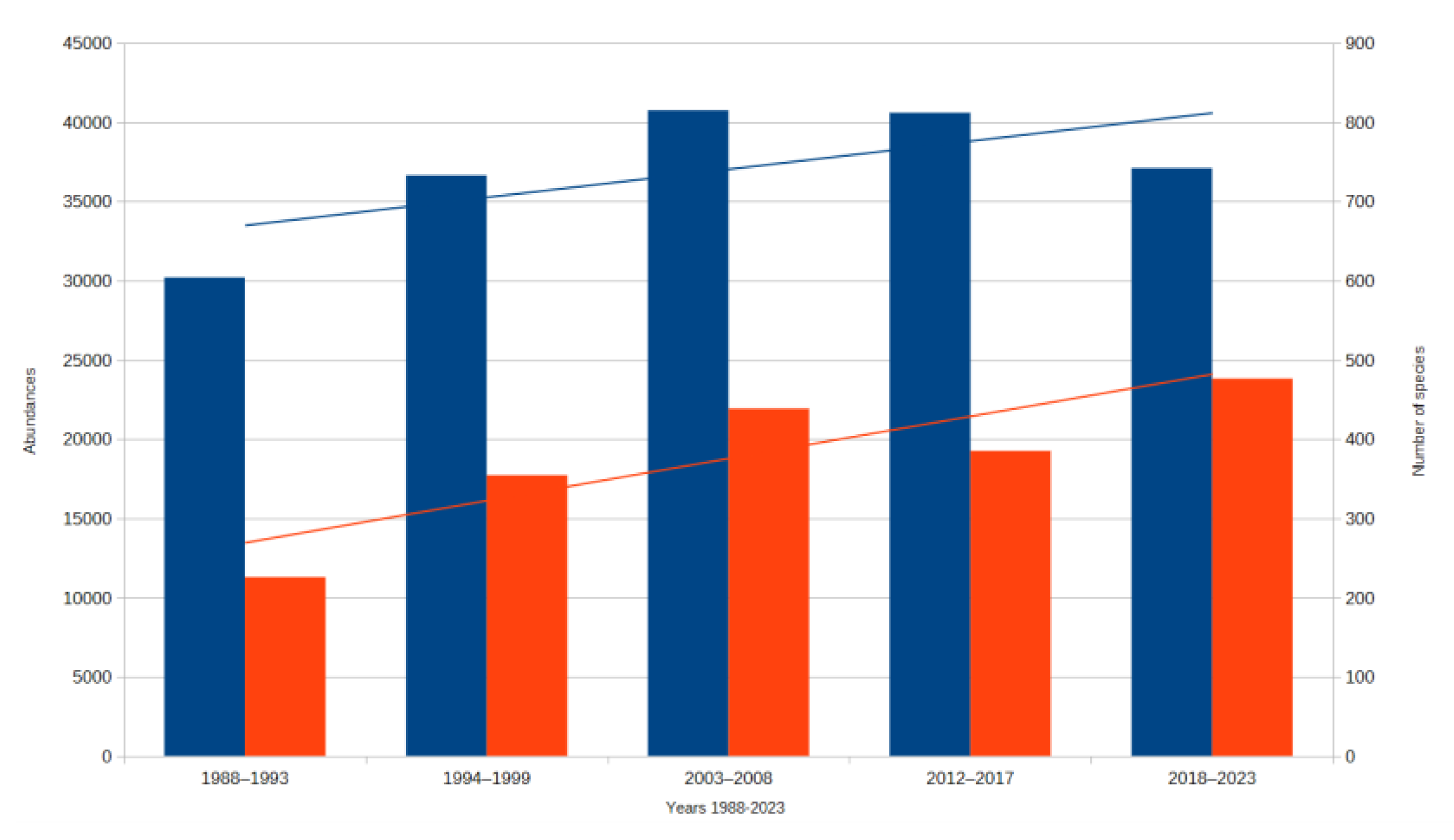
Figure 2.
Trends in abundance and species richness in hoverflies (Diptera) with trendlines (blue: number of species, orange: abundances).
Figure 2.
Trends in abundance and species richness in hoverflies (Diptera) with trendlines (blue: number of species, orange: abundances).
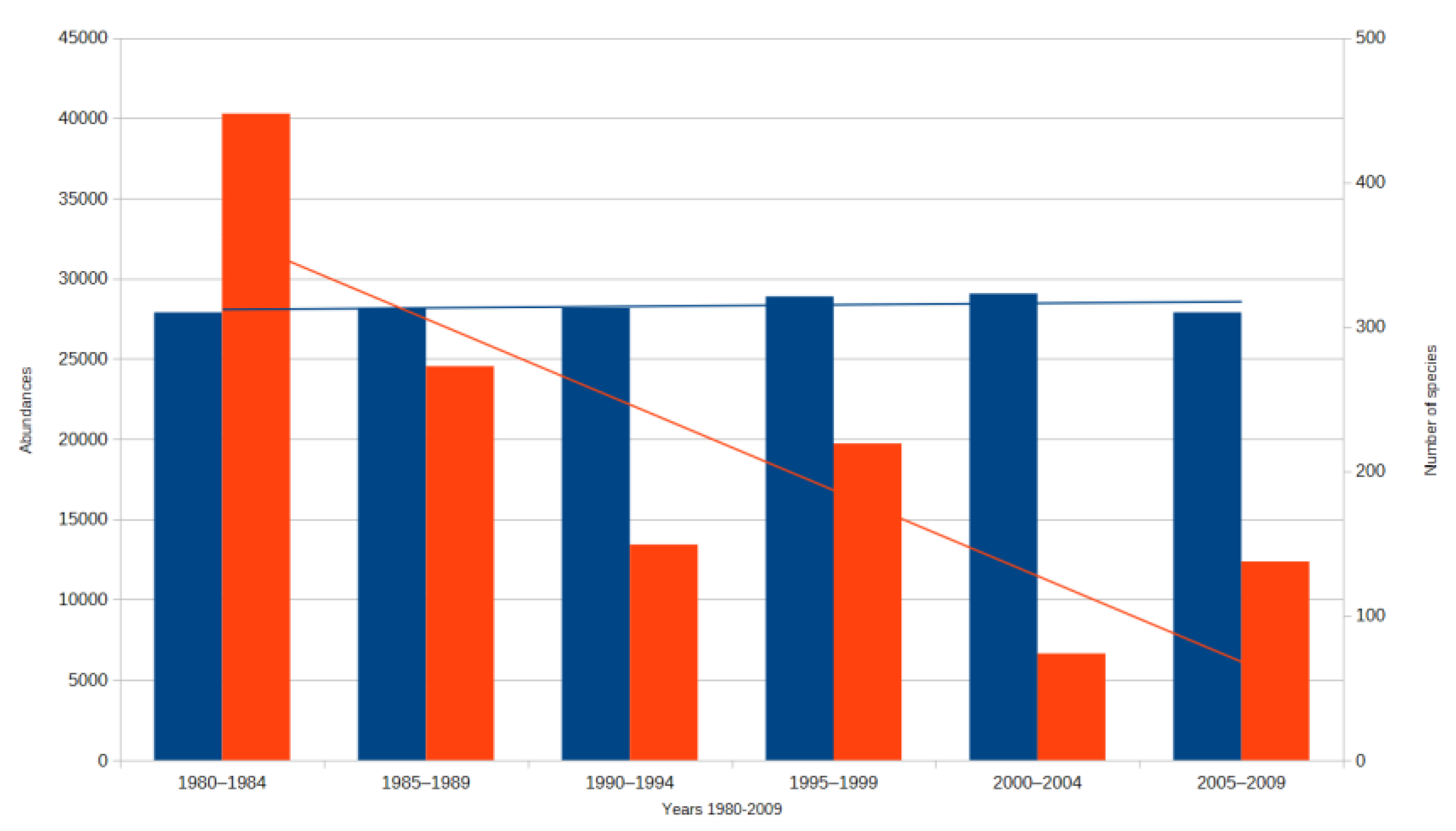
Figure 3.
Trends in abundance and species richness in moths (nocturnal macrolepidoptera) with trendlines (blue: number of species, orange: abundances).
Figure 3.
Trends in abundance and species richness in moths (nocturnal macrolepidoptera) with trendlines (blue: number of species, orange: abundances).
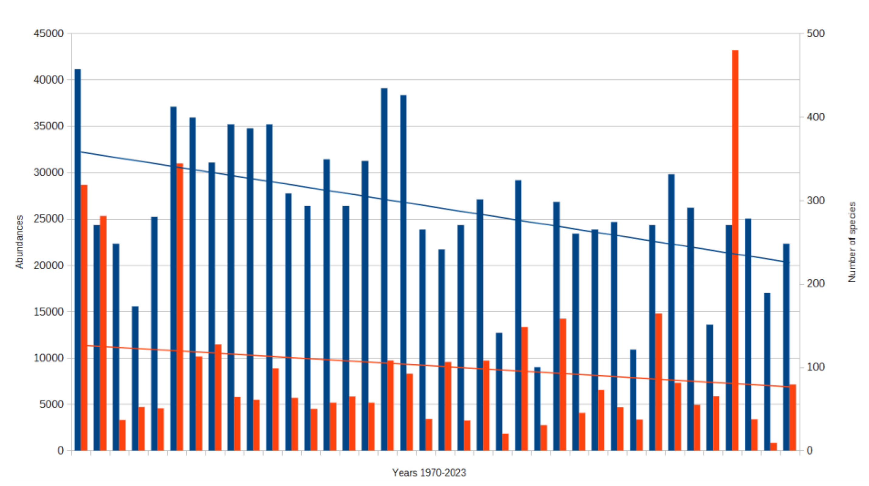

Table 1.
Methodological summary table.
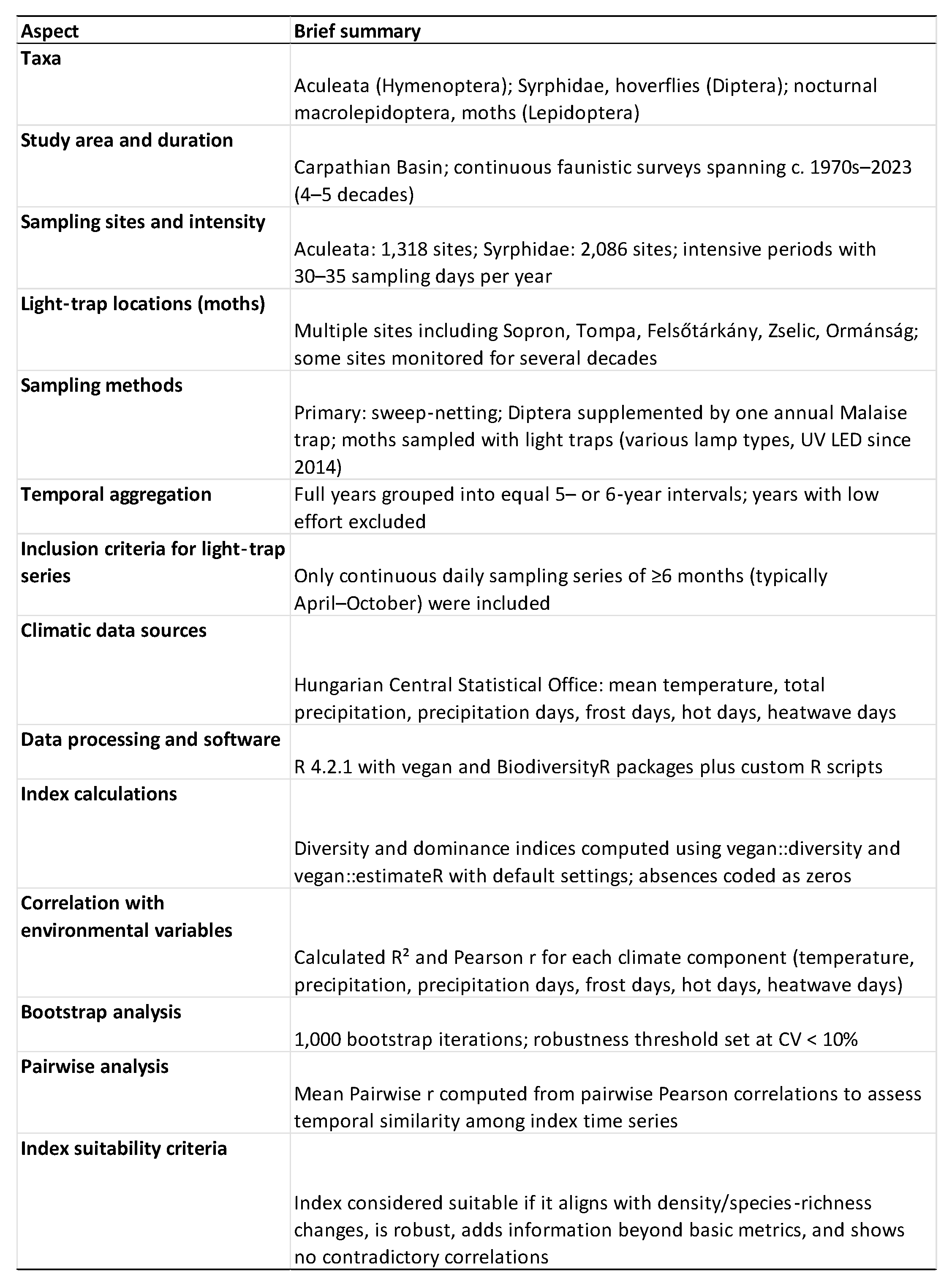 |
Table 2.
Summary of Bootstrap analysis of indices in all groups.
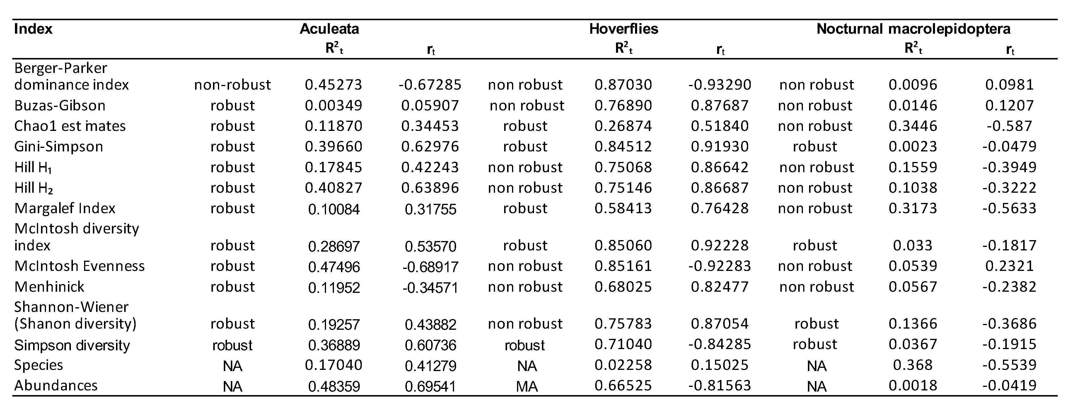 |
Table 3.
Summary of Pairwise analysis of indices in all groups.
 |
Disclaimer/Publisher’s Note: The statements, opinions and data contained in all publications are solely those of the individual author(s) and contributor(s) and not of MDPI and/or the editor(s). MDPI and/or the editor(s) disclaim responsibility for any injury to people or property resulting from any ideas, methods, instructions or products referred to in the content. |
© 2026 by the authors. Licensee MDPI, Basel, Switzerland. This article is an open access article distributed under the terms and conditions of the Creative Commons Attribution (CC BY) license.
Copyright: This open access article is published under a Creative Commons CC BY 4.0 license, which permit the free download, distribution, and reuse, provided that the author and preprint are cited in any reuse.


