

Submitted:
15 February 2026
Posted:
27 February 2026
You are already at the latest version
Abstract
Optimizing crop yield while minimizing energy consumption remains a central challenge in greenhouse horticulture. This study develops an interpretable time-series framework for predicting crop yield and daily energy usage using high-resolution operational and climatic data from a controlledenvironment greenhouse. Four deep learning architectures, including One-Dimensional Convolutional Neural Network (1D-CNN), Long Short-Term Memory Network (LSTM), Bidirectional Long ShortTerm MemoryNetwork(BiLSTM), and TinyTimeMixer (TTM), were evaluated across two varieties of capsicum. LSTM and BiLSTM achieved the highest accuracy for incremental yield prediction, whereas TTM outperformed other models in forecasting daily energy usage, reflecting the distinct temporal characteristics of biological growth and environment-driven energy demand. To uncover the factors driving these predictions, two complementary explainability methods were applied: Gradient SHapley Additive exPlanations (SHAP) for feature-level attribution and a Temporal Convolutional Network with Convolutional Block Attention Module (TCN–CBAM) attention mechanism for joint temporal–feature interpretation. Radiation and drainage-related variables consistently emerged as the dominant contributors to yield, whereas external temperature, and humidity were the primary determinants of energy usage. Temporal attention further showed that yield is influenced by both recent irrigation responses and longer-term developmental dynamics, while energy consumption is driven mainly by short-term climatic fluctuations. These findings provide actionable insights for irrigation scheduling, climate-control strategies, and energy optimization, supporting more transparent and sustainable greenhouse management.
Keywords:
yield prediction
; energy estimation
; explainable artificial intelligence
; greenhouse horticulture
1. Introduction
Greenhouse horticulture is essential for year-round production of high-quality fresh produce, yet it remains one of the most energy-intensive forms of controlled-environment agriculture. Maintaining optimal growing conditions requires continuous operation of heating, cooling, ventilation, and irrigation, all of which substantially increase operational costs and environmental impact [1]. Sustainable production, therefore, depends on accurately predicting and optimizing two core components: incremental crop yield and daily energy usage. In this context, crop yield refers to the weight or volume of produce (measured in grams in this study), whereas energy usage encompasses electricity, nutrient delivery, and other time-varying resource inputs. Balancing the dual objectives of maximizing yield while minimizing energy consumption poses a central challenge in greenhouse operations [2,3]. These processes are further complicated by strong temporal dependencies driven by interactions between internal environmental conditions and external climatic factors.
Recent advances in deep learning have substantially improved the modeling of greenhouse time-series data. Architectures such as 1D Convolutional Neural Networks (1D-CNN) [4], Long Short-Term Memory (LSTM) [5], Bidirectional LSTM (BiLSTM) [6], and transformer-based models such as TinyTimeMixer (TTM) [7] effectively capture nonlinear and multiscale temporal patterns, enabling accurate forecasting of both crop yield and energy usage. However, predictive accuracy alone is insufficient for agricultural applications. Stakeholders require transparent reasoning to verify that model outputs align with biological constraints, greenhouse operational practices, and plant physiological responses. Without such explainability, data-driven recommendations risk misguided irrigation, ventilation, and heating decisions [8].
EXplainable Artificial Intelligence (XAI) addresses this requirement by quantifying feature contributions and revealing the mechanisms underlying model predictions. Gradient SHAP (SHapley Additive exPlanations) [9] offers feature-level attributions that quantify the contribution of environmental and operational variables, while attention-based approaches such as the Temporal Convolutional Network with Convolutional Block Attention Module (TCN–CBAM) [10,11] reveal when key features exert their effects, providing richer temporal–feature insights. Combining these complementary perspectives supports a comprehensive understanding of greenhouse processes by linking model behavior to agronomic reasoning. Such integration is essential for building interpretable, biologically grounded, and operationally reliable decision-support systems in controlled-environment horticulture.
In this study, we integrate advanced time-series modeling with XAI to provide both accurate predictions and interpretable insights for greenhouse horticulture (see Figure 1). Using datasets from Western Sydney University (WSU), we evaluate four deep learning architectures (1D-CNN, LSTM, BiLSTM, and TTM) for incremental yield prediction of capsicum, as well as daily energy usage forecasting. To interpret model behavior, we apply SHAP and a TCN–CBAM framework to quantify feature contributions and their temporal dynamics. Our results highlight the dominant role of irrigation in yield formation, the importance of ventilation and heating parameters in energy consumption, and the time-dependent nature of these interactions. Together, this integrated framework bridges the gap between prediction and interpretation, offering actionable and reliable guidance for sustainable, data-driven greenhouse horticulture management.
2. Materials and Methods
2.1. Facility Configuration
The dataset used in this study was collected from the high-technology glasshouse at the National Vegetable Protected Cropping Centre (NVPCC) located at Western Sydney University (Richmond, NSW, Australia). The greenhouse is a Venlo-type, pad–fan–cooled facility equipped with a fully automated Priva Connext 912 environmental control system (Priva Connext 912, Priva, Netherlands), enabling continuous monitoring and regulation of internal climate conditions. The structure is clad with high-transmission glass and integrates roof vents, thermal screens, fogging, pad–fan cooling, and hot-water pipe heating, providing year-round capability for controlled-environment horticulture.
The compartment used for the capsicum trials during January–June 2022 measured approximately 420 m2, of which approximately 360 m2 were used for active cropping. Cooling was achieved using an evaporative pad–fan system with six exhaust fans (airflow 7000 m−2·h−1 each), while heating was supplied through wall-mounted and ground-level hot-water pipes connected to a gas boiler. These systems were activated automatically according to Priva setpoints based on measured air temperature, relative humidity, and vapour pressure deficit.
An integrated sensor network recorded internal climate variables, external weather conditions, operational signals, as well as energy and water flows at 5-minute intervals. This high-resolution sensing and control infrastructure provided a stable and reproducible platform for modelling greenhouse dynamics and was described in detail in previous publications [12,13].
2.2. Data Description
The study focuses on the capsicum crop cycle conducted between January and June 2022, during which two commercial cultivars (‘Gina’ and ‘YO8366’) were grown on rockwool substrates following standard protected-cropping practices [14,15]. Plants were maintained at 2 stems per plant, giving a crop density of 2.84 plants·m−2. Routine fertigation, canopy management, and integrated pest management were carried out according to industry protocols. Capsicum fruits were harvested twice weekly throughout the production phase (late April to late June 2022).
The predictive targets include:
- Incremental crop yield/weight, reconstructed as a continuous cumulative curve (grams) for each crop; and
- Daily energy usage, representing electrical and thermal loads associated with heating, ventilation, and auxiliary systems.
2.3. Data Preprocessing
Greenhouse telemetry, environmental measurements, energy-usage records, and harvest observations were consolidated into a unified 5-minute time series to ensure temporal comparability across all data sources. Monthly Priva exports were aggregated and aligned using their timestamp fields, after which the combined dataset was cleaned by removing non-informative channels, resolving inconsistencies across files, and standardising variable types. Environmental and operational features exhibiting implausible or out-of-range values were flagged and treated conservatively to avoid introducing artificial dynamics.
Harvest records, which were collected at irregular intervals, were mapped onto the same 5-minute index: cumulative yield curves for capsicum were obtained through linear interpolation between successive harvest events. All projected yield series were clipped to the valid observation window and aligned precisely with the telemetry. This procedure yielded a coherent, temporally synchronised multivariate dataset suitable for feature derivation and downstream modelling.
Feature selection was conducted using mutual information theory to identify dependencies between input variables and the target outcomes. Mutual information measures the amount of information one variable provides about another, helping to identify variables with significant predictive power. Twelve lab-controlled variables, such as irrigation rate, vent temperature, and concentration, were selected to represent internal environmental factors. Additionally, we incorporated eight external weather variables, including temperature, humidity, and solar radiation, to investigate potential connections between greenhouse operations and external climatic conditions (see Figure 2). This comprehensive dataset integrates critical internal and external factors, forming a robust foundation for predictive modeling. A detailed description of all input features is provided in Appendix A.
2.4. Model Architectures
The fine-grained temporal resolution of the dataset requires forecasting models capable of capturing both short- and long-range dependencies underpinning greenhouse yield formation and energy consumption. To this end, we evaluate four state-of-the-art models: 1D-CNN, effective in extracting temporal features; LSTM and BiLSTM, known for their capability to handle sequential data; and TTM, an up-to-date transformer-based model from IBM designed for advanced time-series forecasting. These models were fine-tuned to optimize performance for both incremental yield prediction and non-incremental daily energy usage prediction, reflecting the diverse temporal characteristics of the two tasks.
1D-CNN. The 1D-CNN [4] architecture consists of stacked temporal convolutional layers followed by max-pooling and a fully connected output layer. By applying local receptive fields across time, the model effectively captures short-term temporal fluctuations and high-frequency patterns in environmental and operational signals, making it a computationally efficient baseline for both tasks.
LSTM and BiLSTM. LSTM [5] networks are designed to learn long-range dependencies through gated memory units, making them well suited for modeling the cumulative progression of crop yield. The bidirectional variant (BiLSTM) [6] extends this capability by processing the sequence in both forward and backward directions, enabling richer contextual representation. These models are particularly beneficial for incremental yield prediction, where temporal smoothness and accumulation patterns play a critical role.
TinyTimeMixer (TTM). TTM [7] is a lightweight transformer-inspired architecture developed for time-series forecasting. Instead of self-attention, TTM employs token-mixing operations that efficiently aggregate temporal information across long horizons. This design makes it especially effective for modeling daily energy usage, which is strongly influenced by extended climatic cycles, operational control responses, and long-term greenhouse environment interactions.
Training Configuration. All models were trained using the unified 5-minute time-series dataset and the feature set selected via mutual information analysis. Hyperparameters, including learning rate, batch size, number of convolutional filters or hidden units, and sequence length, were optimized separately for yield and energy forecasting to account for their distinct temporal characteristics. Incremental yield prediction was framed as a cumulative regression task, while daily energy usage was modeled as a non-incremental regression problem. This consistent training protocol ensures fair comparison across architectures while allowing each model to fully leverage its strengths.
2.5. Explainability Methods
To understand how environmental and operational variables contribute to model predictions, we employed two complementary explainability approaches: (i) Gradient SHAP for feature-level attribution, and (ii) a combined TCN–CBAM for joint temporal–feature analysis. Together, these methods provide a multi-perspective explanation of greenhouse dynamics, capturing both which features are most influential and when their effects occur within the prediction window.
Gradient SHAP (Feature-Level Attribution). Gradient SHAP is a gradient-based approximation of SHAP values that combines principles from Integrated Gradients [16] and SmoothGrad within the SHAP framework [9]. It estimates the marginal contribution of each feature by averaging gradients over randomized baselines, producing feature-level attributions that are both locally faithful and globally interpretable. In this study, Gradient SHAP quantifies the relative importance of all input variables for both yield and energy usage prediction, providing a global ranking of influential factors and indicating whether each feature increases or decreases the predicted value, thereby supporting direct agronomic interpretation. We apply Gradient SHAP to all predictive models (1D-CNN, LSTM, BiLSTM, and TTM) to assess the consistency of feature importance across architectures and to obtain model-agnostic estimates of how environmental and operational variables influence predicted outcomes.
TCN-CBAM (Temporal–Feature Attention). While Gradient SHAP identifies which features matter most, it does not reveal when in the input sequence these features exert their influence. To capture temporal sensitivity, we employed an attention-enhanced architecture based on a Temporal Convolutional Network (TCN) [10] integrated with a Convolutional Block Attention Module (CBAM) [11]. The TCN component models multi-scale temporal patterns through dilated convolutions, whereas CBAM generates attention weights across both feature channels and temporal positions. This produces two complementary outputs: (i) a channel-attention map indicating the relative importance of each input variable, and (ii) a temporal-attention curve highlighting the influential time intervals within the input window.
Averaging attention maps across the test set provides global temporal–feature importance profiles, which are compared with SHAP-derived rankings for cross-method validation. The TCN–CBAM explainer is trained on the same input–output pairs as the predictive models (multivariate time series mapped to yield or energy usage) but is not included in predictive performance evaluation. Its purpose is solely to provide an interpretable temporal and feature attention structure that complements the attribution information derived from SHAP.
Complementarity of Explainability Methods. Gradient SHAP and TCN–CBAM together form a unified interpretability framework: SHAP offers reliable feature-level attribution across models, and TCN–CBAM reveals feature–time interaction patterns and long-range temporal sensitivity. This combination enables agronomically meaningful interpretations, such as identifying raditiona and drainage-related variables as dominant drivers of yield and highlighting short-term climatic fluctuations as primary determinants of energy usage. Furthermore, the agreement between these two distinct interpretability paradigms strengthens confidence in the identified drivers and supports biologically grounded explanations of greenhouse crop yield and energy dynamics.
2.6. Evaluation Metric
Model performance was evaluated using two standard quantitative metrics: root mean square error (RMSE) [17] and the coefficient of determination () [18]. RMSE measures the average magnitude of prediction errors, providing an indication of how closely the predicted model values align with the observed data; lower RMSE values correspond to higher predictive accuracy. Meanwhile, quantifies the proportion of variance in the observed data compared to the average value. An score of 1 indicates perfect prediction, 0 means the model performs no better than using the average value as prediction, and negative values signify performance worse than the average. A higher value indicates that the model captures more of the underlying variability in the data.
3. Results
Our experiments span two crop varieties of capsicum. Owing to space limitations, we present the results for Capsicum Gina and the energy usage model in the main text, with full results for the remaining varieties provided in Appendix B. These supplementary analyses exhibit consistent feature-importance rankings and similar temporal-attention patterns, demonstrating that the interpretability findings reported here generalize across cultivars.
3.1. Predictive Performance of Models
We evaluated the predictive performance of the four baseline models, 1D-CNN, LSTM, BiLSTM, and TTM, for both incremental yield prediction and daily energy usage forecasting. Table 1 summarizes the RMSE and values across cultivars and tasks, while Figure 3 and Figure 4 illustrate representative prediction errors for yield and for energy usage.
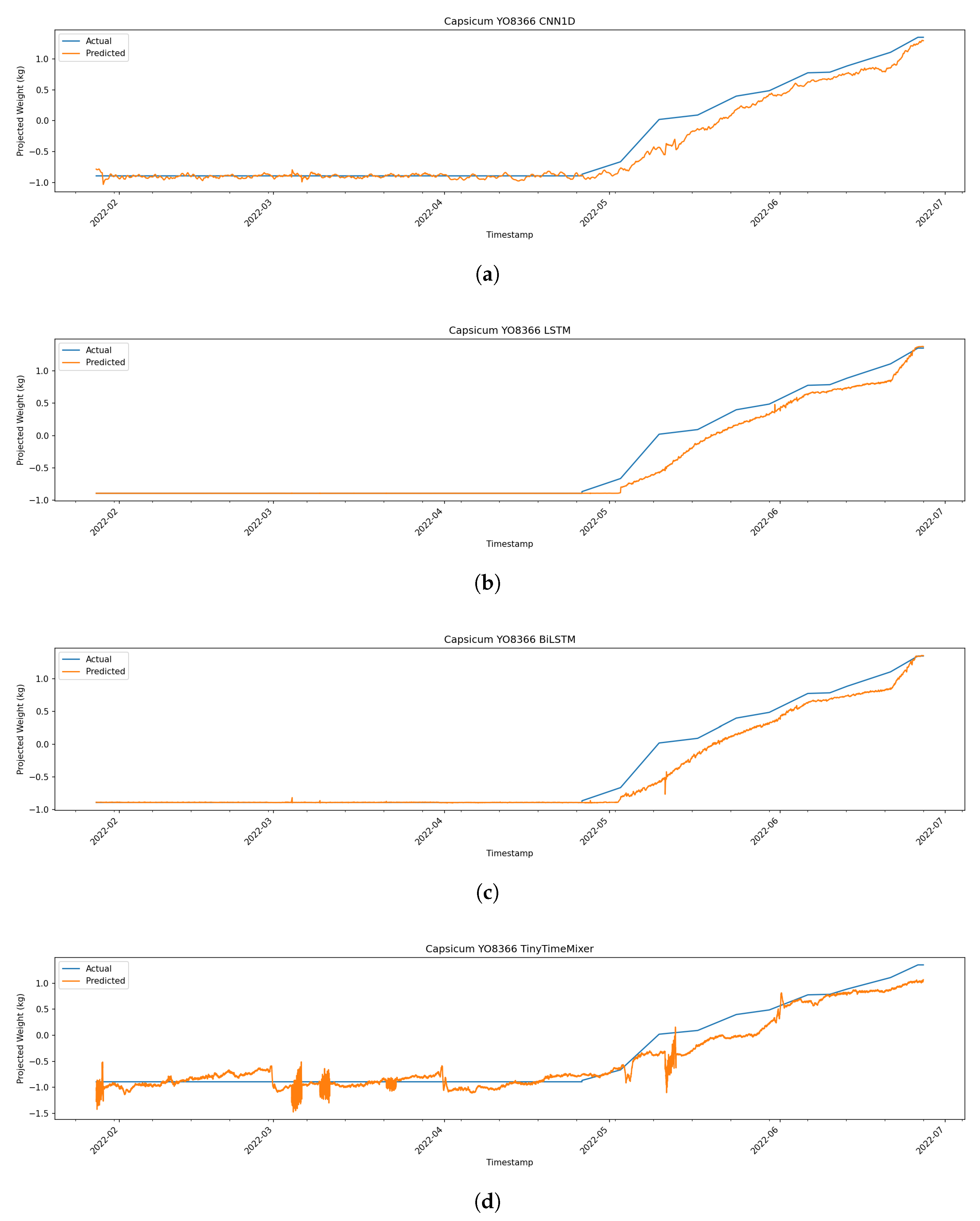
For incremental yield prediction, 1DCNN, LSTM and BiLSTM all achieved promising performance across cultivars (Figure 3). Their structure enables effective modeling of sequential dependencies, which is essential for capturing the cumulative nature of yield formation. Minor prediction fluctuations remain, likely reflecting uncertainties associated with developmental stage transitions and the timing of harvest events.
In contrast, TTM achieved the best accuracy for daily energy usage prediction (Figure 4), benefiting from its ability to model long-range temporal interactions and climate-driven variability. However, TTM exhibited reduced stability when applied to the incremental yield task, suggesting sensitivity to targets with cumulative structure.
Overall, these findings emphasize the importance of aligning model architecture with the temporal characteristics of the target variable: recurrent models are better suited for cumulative crop growth processes, whereas transformer-inspired architectures more effectively capture energy usage patterns driven by external climatic fluctuations.
3.2. Feature-Level Explainability Using Gradient SHAP
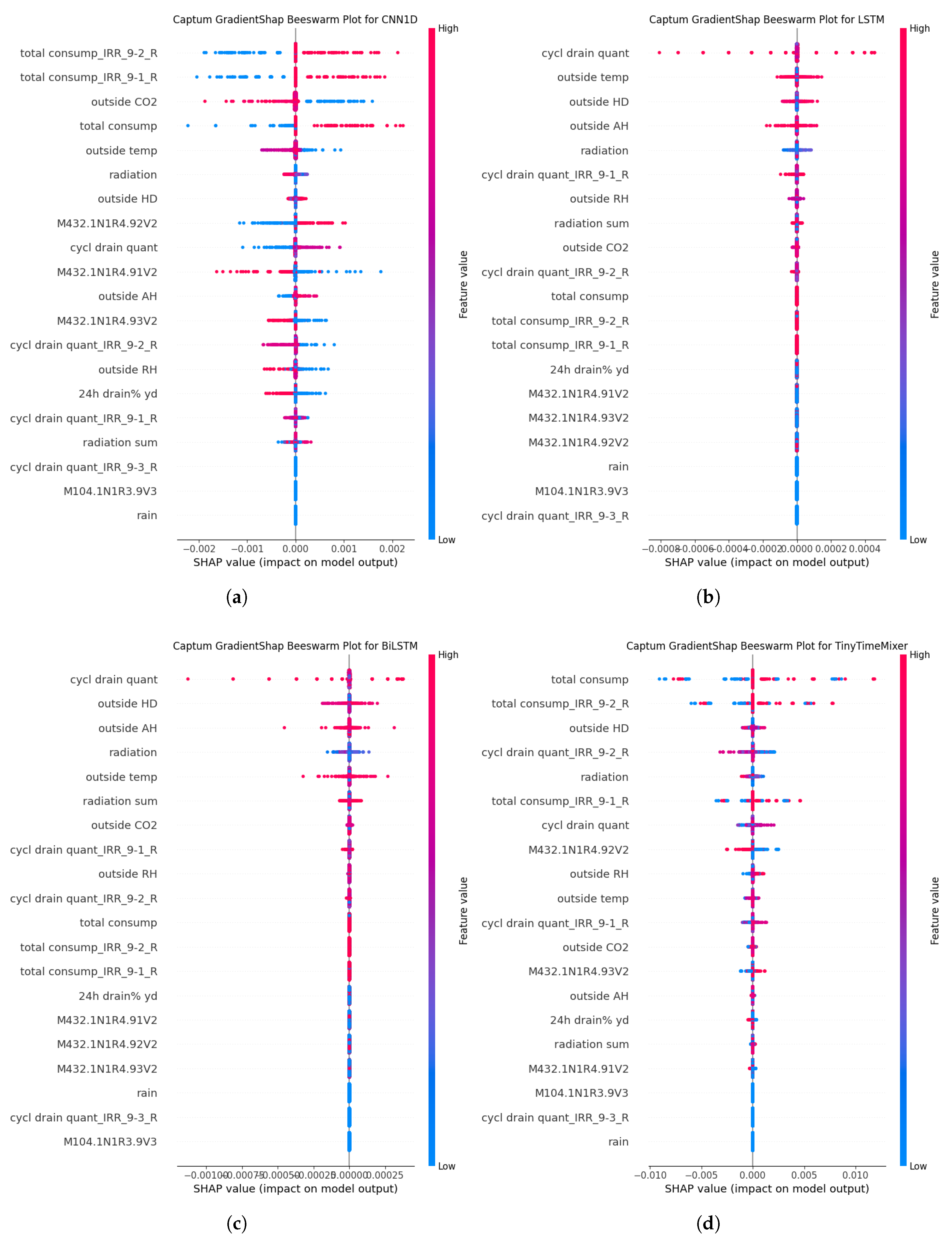
Gradient SHAP was used to quantify the contribution of each environmental and operational variable to the model outputs. Figure 5 and Figure 6 present GradientSHAP beeswarm plots for yield and energy prediction, respectively, across the LSTM, BiLSTM, CNN-1D, and TinyTimeMixer models. In both cases, interpretation is based on the relative spread, density, and directional consistency of SHAP values within each model, rather than on absolute magnitudes.
For yield prediction, the beeswarm plots reveal a consistent attribution structure dominated by radiation and drainage-related variables. Across all architectures, features such as radiation, outside temperature, and humidity-related variables exhibit broad SHAP dispersions and clear deviations from zero, indicating frequent and substantial contributions to yield predictions. Drainage-related variables (e.g., the amount of water drained during each cycle) also show non-negligible SHAP spread, suggesting that root-zone water balance modulates yield responses in conjunction with atmospheric drivers. In contrast, cumulative irrigation consumption and aggregated irrigation totals display comparatively tighter SHAP distributions centred near zero in several models, indicating weaker direct contributions once radiation and microclimate variability are accounted for. Collectively, these patterns suggest that yield formation is primarily radiation- and climate-sensitive, with drainage dynamics acting as an important secondary regulator rather than yield being driven solely by irrigation volume.
For energy usage, the importance profile shifted markedly. SHAP consistently identified external temperature, humidity, and CO2 as the primary predictors. These relationships are physically intuitive: increased temperature differentials drive higher heating or cooling demand, while fluctuations in humidity and CO2 influence ventilation and energy use. The strong agreement between SHAP attributions and known thermodynamic behavior supports the reliability of the predictive models. Operational and irrigation-related variables, by comparison, show narrow SHAP distributions clustered around zero, implying minimal direct impact on energy consumption.
3.3. Temporal–Feature Explainability Using TCN–CBAM
To complement the feature-level interpretations obtained from Gradient SHAP, we further employed a joint temporal–feature attention mechanism based on the combined TCN–CBAM model. This approach provides two forms of explainability: (i) channel attention, highlighting which input variables contribute most to the prediction, and (ii) temporal attention, identifying the most influential time segments within the input window. From a theoretical perspective, temporal attention in the TCN–CBAM framework is expected to highlight temporally localised segments within the input sequence where the model exhibits heightened sensitivity to external conditions, rather than uniformly weighting the entire window. Representative results for Capsicum Gina and energy usage are presented in Figure 7 and Figure 8.
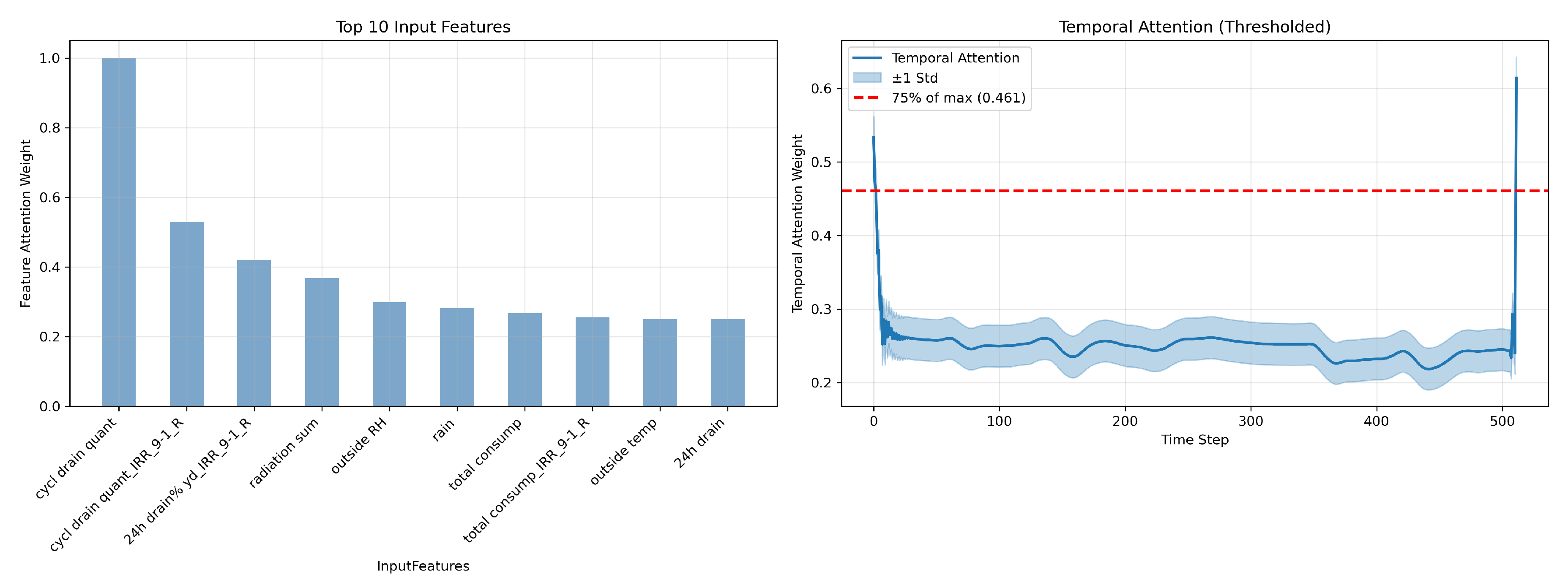
As shown in Figure 7, the channel-attention map (left) indicates that drainage-related variables—such as cycl drain quant, 24h drain%, and IRR-related total consumption—receive the highest attention weights. We also noticed that radiation related features have been assigned moderate importance. This pattern is consistent with Gradient SHAP results and aligns with agronomic knowledge that radiation and irrigation dynamics heavily regulate fruit development in controlled environments.
The temporal-attention curve (right) reveals two prominent high-attention regions: an early-window activation shortly after the prediction window begins, and a second region aligned with later phases of the crop cycle. These intervals likely correspond to distinct physiological growth stages or recent irrigation responses, suggesting that both short-term and accumulated temporal effects play a role in yield formation
Figure 8 shows the attention patterns learned for energy usage. Unlike the yield task, the most influential features are dominated by climate-related and heating variables, including outside temperature, outside AH, outside RH, and outside CO2. This contrast highlights the fundamentally different drivers of energy expenditure in greenhouses compared with crop growth.
The temporal-attention curve displays a distinctly different pattern from the yield task: high-attention segments occur toward the end of the input window, suggesting that recent climatic fluctuations and operational control actions (e.g., heating or ventilation responses) immediately preceding the forecast time have the largest influence on energy consumption.
Overall, the TCN–CBAM results demonstrate strong consistency with Gradient SHAP, while additionally revealing when important features exert their influence. This temporal–feature perspective provides a richer interpretation of greenhouse dynamics, capturing both environmental sensitivities and crop physiological dependencies.
4. Discussion
Consistency Across Explainability Methods. The combination of Gradient SHAP and the TCN–CBAM attention mechanism provides a coherent and mutually reinforcing interpretation of model behavior. Gradient SHAP offers global feature-level attribution, whereas TCN–CBAM supplies a joint temporal–feature perspective [19,20]. Across both yield and energy prediction tasks, the highest-ranked features identified by CBAM share similarity with the SHAP-derived importance orderings, such as cycl drain quant and radiation, demonstrating strong consistency between gradient-based and attention-based interpretability. At the same time, TCN–CBAM adds an additional layer of explanatory depth by revealing when important features exert their influence, thereby capturing short-term responses and longer-term temporal dependencies that SHAP alone cannot characterize. This can explain some high-ranked features identified by CBAM do not match the SHAP-derived importance orderings. While SHAP is designed to estimate the average marginal contribution of individual features to the model output (relative to a background distribution), TCN-CBAM attention reflects where and when the model focuses internally to form its prediction. As a result, features that act mainly through temporal interactions, short but critical windows, or correlated effects with other climate variables may receive strong attention weights without necessarily ranking highly in SHAP importance. In our case, variables such as 24h drain in yield and rain in energy appear to influence prediction primarily through timing-specific effects and interactions (e.g., with temperature or radiation), which are captured by the temporal attention mechanism but can be diluted in SHAP due to feature correlation and attribution sharing. Therefore, the two methods are not contradictory, but rather provide complementary perspectives on feature relevance and also underscore the importance of using SHAP with TCN-CBAM as SHAP alone may have not identified features correctly. This complementarity highlights the advantages of integrating multiple XAI techniques to obtain a more holistic understanding of greenhouse dynamics.
Agronomic Insights. The explainability results yield several insights aligned with established greenhouse horticulture principles. For yield prediction, both SHAP and CBAM consistently highlight radiation and drainage-related variables—such as drainage fraction and irrigation consumption—were identified as the most influential predictors. This agrees with agronomic understanding that radiation-related features contribute to photosynthesis and biomass accumulation [21,22], while irrigation scheduling and water–nutrient delivery strongly regulate fruit development, root-zone health, and vegetative–reproductive balance [23,24]. Other external atmospheric variables play differentiated roles: humidity exhibit broader attribution distributions, indicating sensitivity of yield to microclimate regulation [25], whereas rainfall shows limited direct attribution, reflecting the buffering effects of controlled-environment cultivation [26]. In contrast, energy usage prediction is dominated by climate-related variables, including external temperature, CO2, and humidity, as well as heating-water consumption. These findings match thermodynamic expectations: larger discrepancies between outdoor and indoor conditions increase heating or cooling demands, while CO2 and humidity levels influence ventilation strategies [27,28]. The clear separation between yield drivers and energy drivers reinforces the need for multi-objective greenhouse management, as improving one outcome does not necessarily optimize the other [29,30].
Scientific Implications. The dual-perspective interpretability obtained in this study illustrates how feature-level and temporal-level explanations together enhance transparency in agricultural AI systems [31,32]. Feature-level attribution identifies the primary input variables influencing model outputs, enabling domain experts to verify that learning patterns are biologically and physically plausible. Temporal attention further reveals the time periods during which greenhouse processes are most sensitive, offering clues about crop developmental phases, short-term irrigation responses, or climate-driven operational adjustments. The strong coherence across XAI methods strengthens trust in the predictive models, supporting their potential deployment within decision-support tools for sustainable controlled-environment agriculture. More broadly, the methodological framework demonstrates how time-series explainability can be extended beyond static feature rankings to capture dynamic system behavior.
Limitations. Several limitations should be acknowledged. First, the dataset originates from a single greenhouse facility, and cross-greenhouse generalizability has not yet been validated. Differences in cultivation systems, crop varieties, climate zones, and management practices may affect model transferability. Second, although the selected feature set captures major environmental and operational variables, spatial information (e.g., canopy-level microclimate variability) and multimodal data (e.g., imagery or physiological sensing) were not included. Such modalities could enhance both predictive accuracy and interpretability. Third, the temporal-attention patterns identified by TCN–CBAM reflect learned associations rather than causal relationships; careful validation with agronomic experiments is required to substantiate causal interpretations.
Future Work. Future efforts may extend this work along several directions. Integrating additional interpretability techniques, such as Grad-CAM or Integrated Gradients within convolutional architectures, could provide complementary visualizations of temporal saliency. Cross-regional and cross-facility evaluations will be essential to assess model robustness under diverse climatic and management regimes. Furthermore, combining temporal and feature-level explainability with causal modeling frameworks may enable stronger mechanistic interpretations of crop–environment interactions. Finally, incorporating multimodal data streams—such as thermal imagery, leaf temperature measurements, or soil moisture sensing—could further enhance both predictive performance and physiological interpretability.
5. Conclusions
This study presented an interpretable time-series modeling framework for predicting crop yield and energy usage in greenhouse horticulture. By evaluating four deep learning architectures, including 1D-CNN, LSTM, BiLSTM, and TTM, we showed that the optimal predictive model depends on the temporal characteristics of the target variable: recurrent networks (LSTM and BiLSTM) excelled in incremental yield prediction, whereas TTM achieved the highest accuracy for daily energy usage forecasting.
Beyond achieving strong predictive performance, we integrated Gradient SHAP and a TCN–CBAM attention mechanism to provide complementary feature-level and temporal–feature explanations. Across all crop varieties, radiation and drainage-related variables variables were identified as the primary drivers of yield formation, while energy consumption was governed mainly by external climatic factors, particularly outside temperature, humidity, and CO2. Temporal attention further revealed distinct dynamic patterns underlying the two tasks, with yield influenced by both recent irrigation events and longer-term developmental trends, and energy usage dominated by short-term climatic fluctuations.
These results demonstrate that combining deep learning with multi-level explainability yields transparent and agronomically meaningful insights. The proposed framework provides practical guidance for optimizing irrigation scheduling, climate control, and energy management, supporting more efficient and sustainable greenhouse operations. Future work will focus on evaluating cross-greenhouse generalization, incorporating multimodal sensing data, and developing causal modeling approaches to further improve the robustness and interpretability of greenhouse AI systems.
Appendix A. Description of Input Features
Table A1 lists the 20 input features selected for model training and explainability analysis. These variables represent key operational, environmental, and climatic factors relevant to greenhouse crop production.

Table A1.
Description of the 20 selected features used as model inputs.
| Feature Name | Units | Description |
|---|---|---|
| 24h dose | The water dose in litres per greenhouse area after the 24-hour period transition for Today. No valve group specified. | |
| 24h drain% yd_IRR_9-1_R | % | The average drain percentage after the 24-hour period transition for yesterday for valve group 9.1. |
| measured value | It is the measured value of the vent/curtain position in from the positioning unit on the gearbox. | |
| cycl drain quant | It is the amount of water drained during each cycle. It is measured each cycle. | |
| cycl drain quant_IRR_9-3_R | Volume of water drained during each irrigation cycle for valve group 9.3. | |
| cycl drain quant_IRR_9-1_R | Total irrigation water consumption per square meter for valve group 9.1 over the previous 24-hour period. | |
| M432.1N1R4.92V2 | The consumption of valve group 9.2 in for yesterday (24hr period) | |
| M104.1N1R3.9V3 | The supplied accumulated energy usage of the compartment water temperatures and the connected autonomous water temperatures, related to surface compartment for C9 for yesterday. | |
| M432.1N1R4.91V2 | The consumption of valve group 9.1 in for yesterday (24hr period) | |
| M432.1N1R4.93V2 | The consumption of valve group 9.3 in for yesterday (24hr period). | |
| total consump | It is the total amount of irrigation that the plants take up per . | |
| total consump_IRR_9-2_R | The total consumption of valve group 9.2 in . The total consumption is adjustable and the count continues from the modification. This allows you to register the quantity in of an entire crop or crop phase. | |
| outside AH | g/m3 | Outside Absolute Humidity |
| outside CO2 | ppm | Outside CO2 levels |
| outside HD | Outside Humidity Deficit | |
| outside RH | % | Outside Relative Humidity |
| outside temp | °C | Outside air temperature |
| radiation | Instantaneous incoming solar radiation measured outside the greenhouse. | |
| radiation sum | Daily accumulated solar radiation outside the greenhouse. | |
| rain | Binary | Binary indicator representing the occurrence of rainfall events. |
Appendix B. Additional Experimental Results
This appendix provides the full set of predictive and interpretability results for all crop varieties evaluated in this study. The patterns observed for these varieties are consistent with those presented in the main text for Capsicum Gina and the energy usage model. For each variety, we include: (i) predictive performance plots for all four baseline models, and (ii) Gradient SHAP and TCN–CBAM explainability visualizations for both yield and energy usage (where applicable).
Appendix B.1. Capsicum YO8366
Appendix B.1.1. Predictive Performance
Figure A1.
Time-series model performance on predicting Capsicum YO8366 yield. (a) 1D-CNN yield forecasting performance. (b) LSTM yield forecasting performance. (c) BiLSTM yield forecasting performance. (d) TTM yield forecasting performance.
Figure A1.
Time-series model performance on predicting Capsicum YO8366 yield. (a) 1D-CNN yield forecasting performance. (b) LSTM yield forecasting performance. (c) BiLSTM yield forecasting performance. (d) TTM yield forecasting performance.
Appendix B.1.2. Gradient SHAP Explainability
Figure A2.
Gradient SHAP feature importance for Capsicum YO8366. (a) 1D-CNN, (b) LSTM, (c) BiLSTM, (d) TTM.
Figure A2.
Gradient SHAP feature importance for Capsicum YO8366. (a) 1D-CNN, (b) LSTM, (c) BiLSTM, (d) TTM.
Appendix B.1.3. TCN–CBAM Attention
Figure A3.
TCN–CBAM explainability for Capsicum YO8366: (left) top input-feature attention weights; (right) temporal attention curve with high-importance intervals highlighted.
Figure A3.
TCN–CBAM explainability for Capsicum YO8366: (left) top input-feature attention weights; (right) temporal attention curve with high-importance intervals highlighted.
References
- Samaranayake, P.; Liang, W.; Chen, Z.H.; Tissue, D.; Lan, Y.C. Sustainable protected cropping: A case study of seasonal impacts on greenhouse energy consumption during capsicum production. Energies 2020, 13, 4468. [Google Scholar] [CrossRef]
- Wang, Z.; Bao, A.; Li, J.; He, J.; Wang, K.; Wang, X.; Sun, X. Study on the Effect of Non-Uniform Ventilation on Energy and Plant Growth in a Greenhouse. Horticulturae 2025, 11, 166. [Google Scholar] [CrossRef]
- Villagrán, E.; Romero-Perdomo, F.; Numa-Vergel, S.; Galindo-Pacheco, J.R.; Salinas-Velandia, D.A. Life Cycle Assessment in Protected Agriculture: Where Are We Now, and Where Should We Go Next? Horticulturae 2023, 10, 15. [Google Scholar] [CrossRef]
- Wang, X.; Mao, D.; Li, X. Bearing fault diagnosis based on vibro-acoustic data fusion and 1D-CNN network. Measurement 2021, 173, 108518. [Google Scholar] [CrossRef]
- Graves, A. Long short-term memory. In Supervised sequence labelling with recurrent neural networks; 2012; pp. 37–45. [Google Scholar]
- Huang, Z.; Xu, W.; Yu, K. Bidirectional LSTM-CRF models for sequence tagging. arXiv 2015, arXiv:1508.01991. [Google Scholar] [CrossRef]
- Ekambaram, V.; Jati, A.; Dayama, P.; Mukherjee, S.; Nguyen, N.H.; Gifford, W.M.; Reddy, C.; Kalagnanam, J. Tiny Time Mixers (TTMs): Fast Pre-trained Models for Enhanced Zero/Few-Shot Forecasting of Multivariate Time Series. CoRR 2024. [Google Scholar]
- Wang, Z.; Liu, K.; Liang, L.; Li, C.; Ji, T.; Xu, J.; Liu, H.; Diao, M. An Explainable Machine Learning Framework for the Hierarchical Management of Hot Pepper Damping-Off in Intensive Seedling Production. Horticulturae 2025, 11, 1258. [Google Scholar] [CrossRef]
- Lundberg, S.M.; Lee, S.I. A unified approach to interpreting model predictions. Advances in neural information processing systems 2017, 30. [Google Scholar]
- Lea, C.; Flynn, M.D.; Vidal, R.; Reiter, A.; Hager, G.D. Temporal convolutional networks for action segmentation and detection. In Proceedings of the proceedings of the IEEE Conference on Computer Vision and Pattern Recognition, 2017; pp. 156–165. [Google Scholar]
- Woo, S.; Park, J.; Lee, J.Y.; Kweon, I.S. Cbam: Convolutional block attention module. In Proceedings of the Proceedings of the European conference on computer vision (ECCV), 2018; pp. 3–19. [Google Scholar]
- He, J.; Lin, T.; Liang, W.; Chavan, S.; Sethuvenkatraman, S.; Goldsworthy, M.; Tissue, D.; Chen, Z.H. Energy and fertigation consumption and economic viability of a light blocking film in greenhouse lettuce production. Journal of Cleaner Production 2024, 479, 144013. [Google Scholar] [CrossRef]
- Lin, T.; Maier, C.R.; Liang, W.; Klause, N.; He, J.; Tissue, D.T.; Lan, Y.C.; Sethuvenkatraman, S.; Goldsworthy, M.; Chen, Z.H. A light-blocking greenhouse film differentially impacts climate control energy use and capsicum production. Frontiers in Energy Research 2024, 12, 1360536. [Google Scholar] [CrossRef]
- Islam, M.M.; He, J.; Yong, M.; Babla, M.; Liang, W.; Li, L.; Bose, J.; Donovan-Mak, M.; Huda, S.; Tissue, D.; et al. Reduced fertigation input sustains yield and physiological performance for improved economic returns and cleaner production of greenhouse eggplant. Scientia Horticulturae 2024, 331, 113097. [Google Scholar] [CrossRef]
- Sonali; He, J.; Wang, Y.; Liang, W.; Rasouli, F.; Li, L.; Bose, J.; Donovan-Mak, M.; Huda, S.; Jayasena, V.; et al. Optimised fertigation improves yield and quality of cucumbers for resource efficiency and economic return in high-tech greenhouses. Journal of Agriculture and Food Research 2025, 19, 101699. [Google Scholar] [CrossRef]
- Sundararajan, M.; Taly, A.; Yan, Q. Axiomatic attribution for deep networks. In Proceedings of the International conference on machine learning; PMLR, 2017; pp. 3319–3328. [Google Scholar]
- Hodson, T.O. Root mean square error (RMSE) or mean absolute error (MAE): When to use them or not. Geoscientific Model Development Discussions 2022, 2022, 1–10. [Google Scholar] [CrossRef]
- Di Bucchianico, A. Coefficient of determination (R 2). Encyclopedia of statistics in quality and reliability 2008. [Google Scholar]
- Hinterleitner, A.; Bartz-Beielstein, T.; Schulz, R.; Spengler, S.; Winter, T.; Leitenmeier, C. Enhancing feature selection and interpretability in AI regression tasks through feature attribution. arXiv 2024, arXiv:2409.16787. [Google Scholar] [CrossRef]
- Ding, N.; Yang, Y.; Tan, P.; Dong, Z.; Zhang, K.; Shi, Y. Research on intelligent diagnosis of multi-modal piston axis wear state based on FMD and resnet-CBAM-TCN spatio-temporal architecture. Engineering Research Express 2025, 7, 035417. [Google Scholar] [CrossRef]
- Monteith, J.L. Climate and the efficiency of crop production in Britain. Philosophical transactions of the royal society of London. B, Biological Sciences 1977, 281, 277–294. [Google Scholar] [CrossRef]
- Taiz, L.; Møller, I.M.; Murphy, A.; Zeiger, E. Plant physiology and development. (No Title) 2023. [Google Scholar]
- Dorais, M.; Papadopoulos, A.; Gosselin, A. Greenhouse tomato fruit quality. Horticultural reviews 2002, 26, 239–319. [Google Scholar]
- Gu, Z.; Qi, Z.; Burghate, R.; Yuan, S.; Jiao, X.; Xu, J. Irrigation scheduling approaches and applications: A review. Journal of Irrigation and Drainage Engineering 2020, 146, 04020007. [Google Scholar] [CrossRef]
- García-Mañas, F.; Hägglund, T.; Guzmán, J.L.; Rodríguez, F.; Berenguel, M. A practical solution for multivariable control of temperature and humidity in greenhouses. European Journal of Control 2024, 77, 100967. [Google Scholar] [CrossRef]
- Soussi, M.; Chaibi, M.T.; Buchholz, M.; Saghrouni, Z. Comprehensive review on climate control and cooling systems in greenhouses under hot and arid conditions. Agronomy 2022, 12, 626. [Google Scholar] [CrossRef]
- Shamshiri, R.; Ismail, W.I.W. A review of greenhouse climate control and automation systems in tropical regions. J. Agric. Sci. Appl 2013, 2, 176–183. [Google Scholar] [CrossRef]
- Halling, M. Greenhouse Energy Balance: A numerical approach to analyse the influence of location, season, and structural design of greenhouses. 2024. [Google Scholar]
- Van Beveren, P.; Bontsema, J.; Van Straten, G.; Van Henten, E. Optimal control of greenhouse climate using minimal energy and grower defined bounds. Applied Energy 2015, 159, 509–519. [Google Scholar] [CrossRef]
- Tomar, A. Multi-objective optimization of photovoltaic greenhouses with modelling and field validation. Solar Energy 2025, 301, 113938. [Google Scholar] [CrossRef]
- Rudin, C. Stop explaining black box machine learning models for high stakes decisions and use interpretable models instead. Nature machine intelligence 2019, 1, 206–215. [Google Scholar] [CrossRef] [PubMed]
- Guidotti, R.; Monreale, A.; Ruggieri, S.; Turini, F.; Giannotti, F.; Pedreschi, D. A survey of methods for explaining black box models. ACM computing surveys (CSUR) 2018, 51, 1–42. [Google Scholar] [CrossRef]
Figure 1.
Workflow integrating time-series modeling with feature and temporal–feature explainability.
Figure 1.
Workflow integrating time-series modeling with feature and temporal–feature explainability.
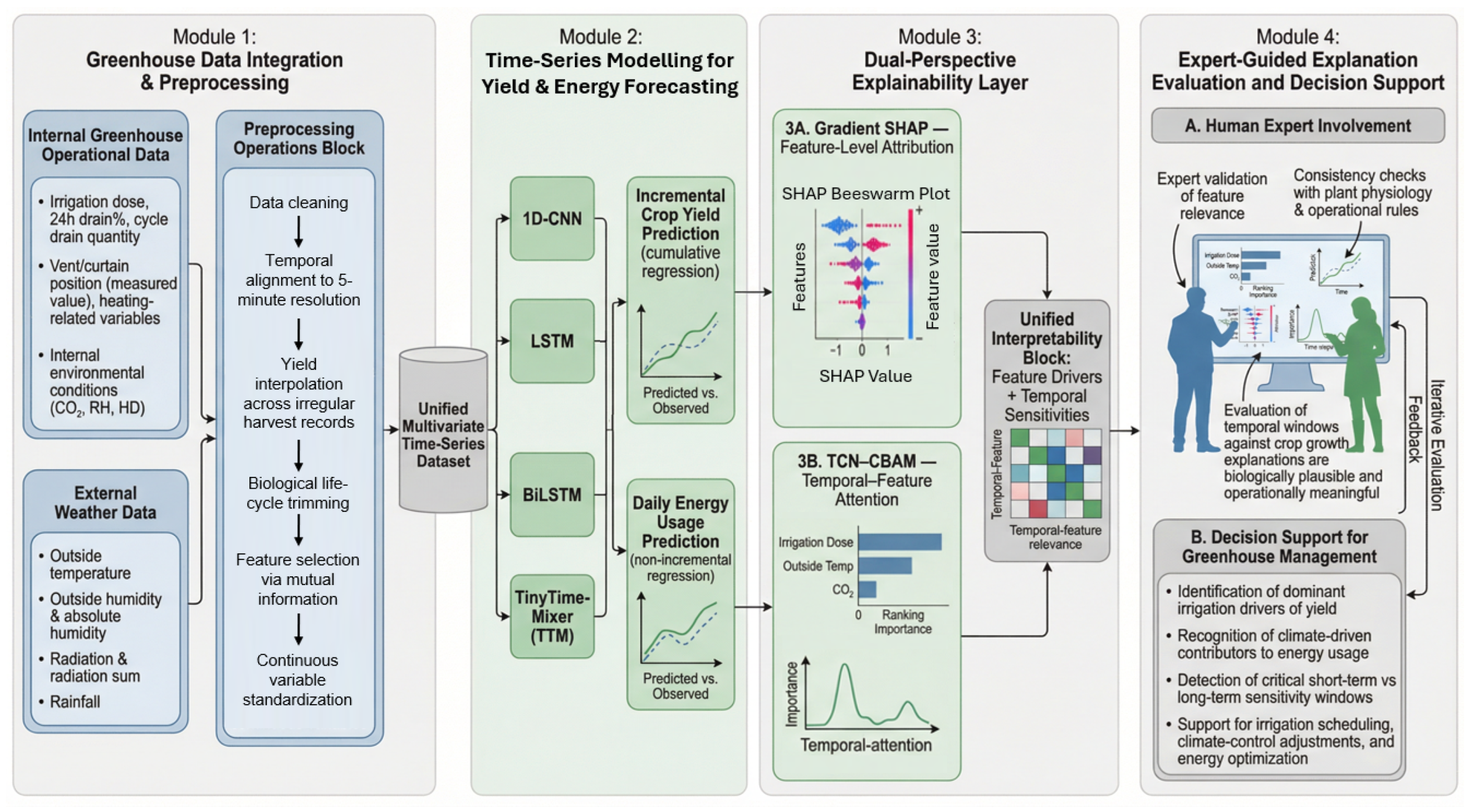
Figure 2.
Correlation matrix of input features for capsicum Gina and energy consumption modeling. (a) Correlation matrix for Capsicum Gina. (b) Correlation matrix for energy consumption.
Figure 2.
Correlation matrix of input features for capsicum Gina and energy consumption modeling. (a) Correlation matrix for Capsicum Gina. (b) Correlation matrix for energy consumption.
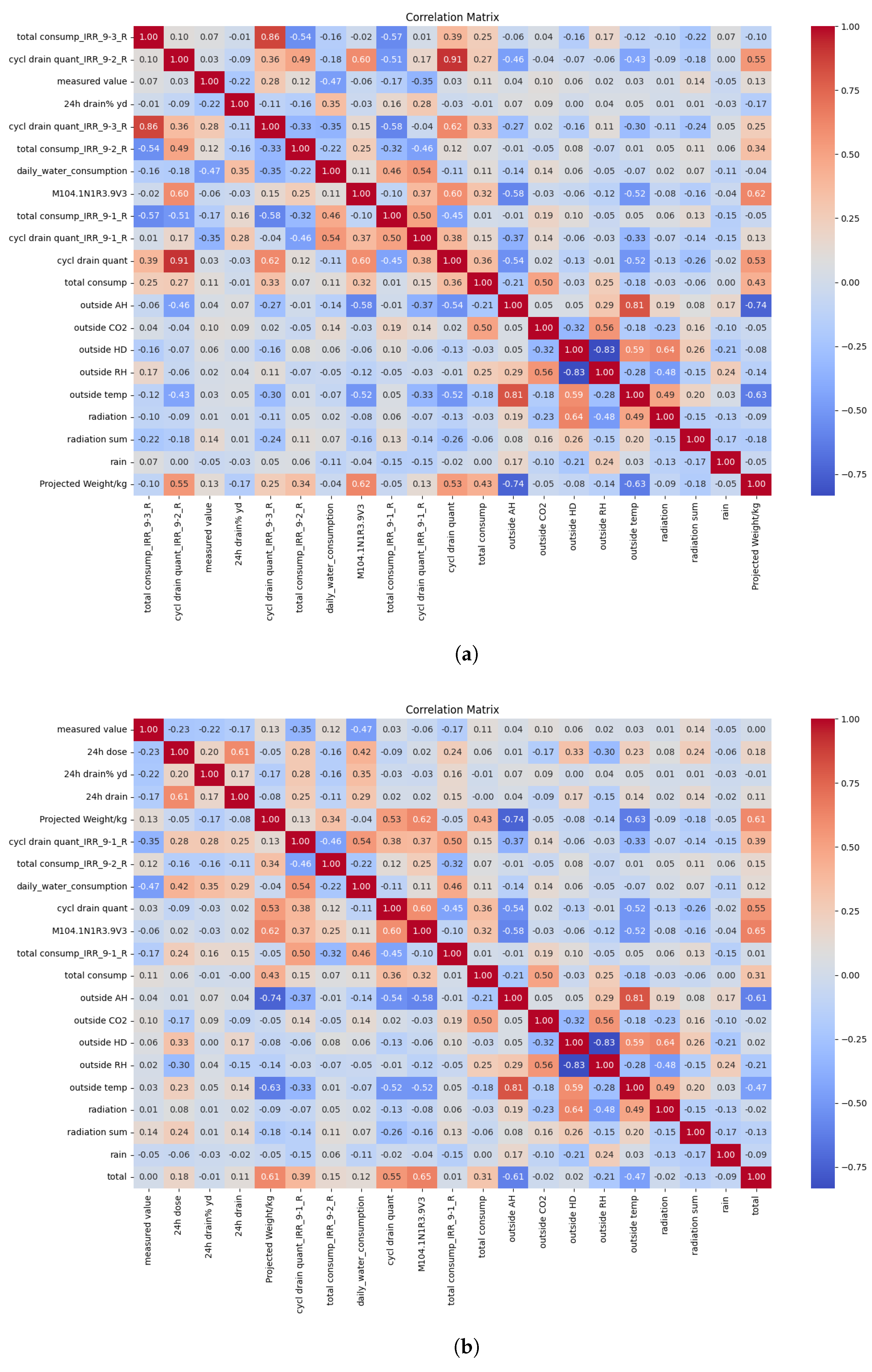
Figure 3.
Time-series model performance on predicting capsicum Gina yield. (a) 1D-CNN yield forecasting performance. (b) LSTM yield forecasting performance. (c) BiLSTM yield forecasting performance. (d) TTM yield forecasting performance.
Figure 3.
Time-series model performance on predicting capsicum Gina yield. (a) 1D-CNN yield forecasting performance. (b) LSTM yield forecasting performance. (c) BiLSTM yield forecasting performance. (d) TTM yield forecasting performance.
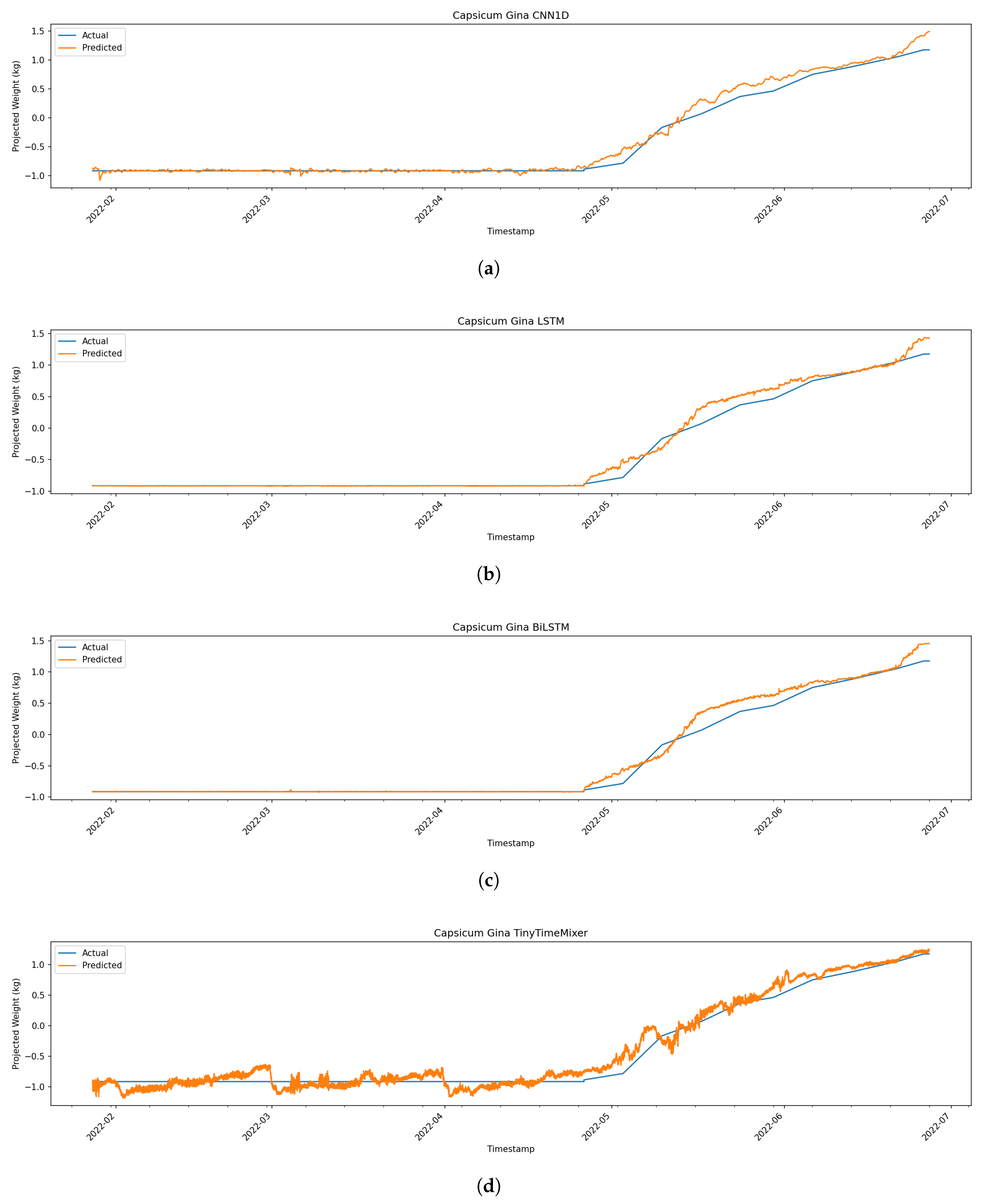
Figure 4.
Time-series model performance on predicting energy usage. (a) 1D-CNN energy cost prediction. (b) LSTM energy cost prediction. (c) BiLSTM energy cost prediction. (d) TTM energy cost prediction.
Figure 4.
Time-series model performance on predicting energy usage. (a) 1D-CNN energy cost prediction. (b) LSTM energy cost prediction. (c) BiLSTM energy cost prediction. (d) TTM energy cost prediction.
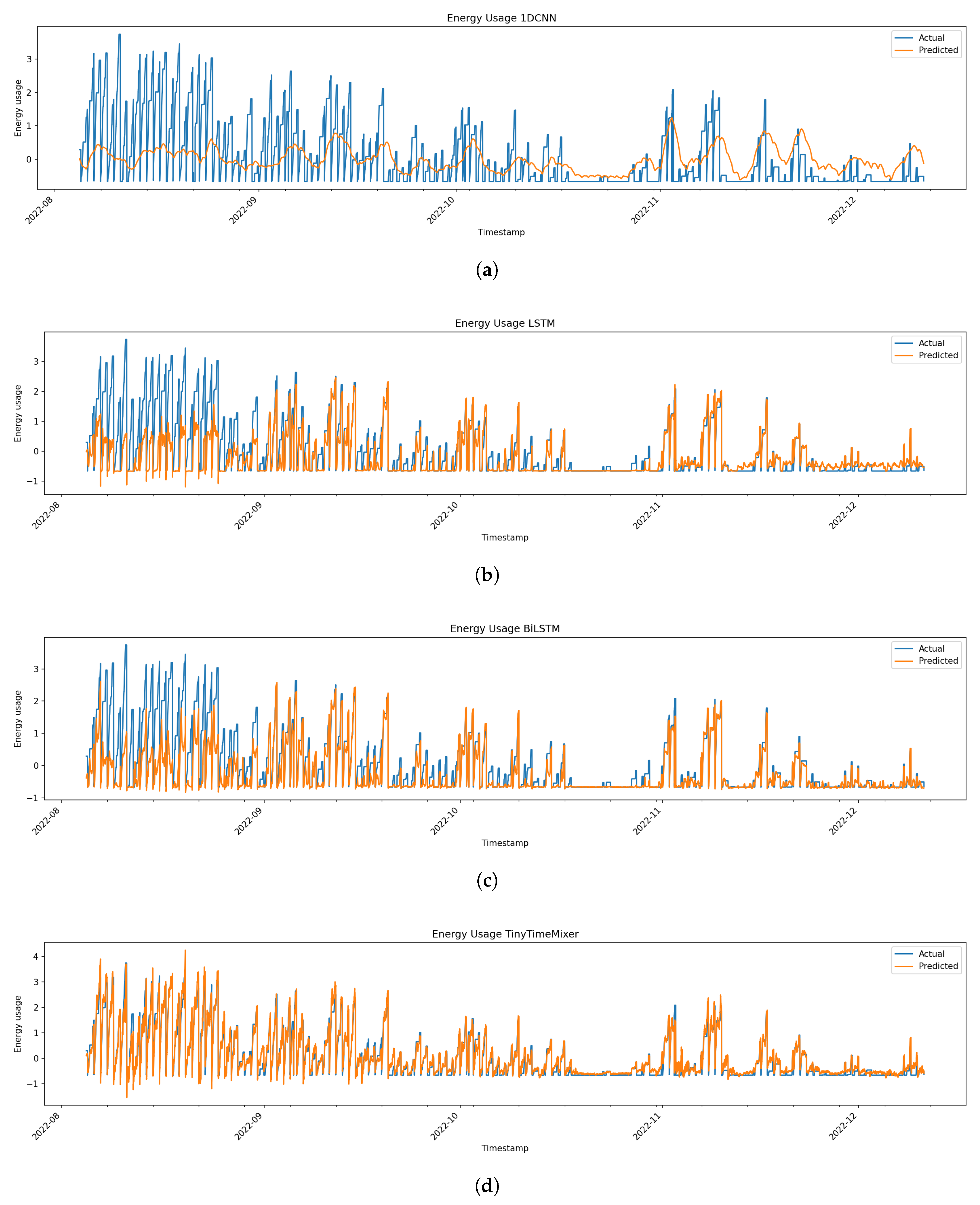
Figure 5.
Explanations for time-series model performance on predicting crop yield. (a) 1D-CNN, (b) LSTM, (c) BiLSTM, (d) TTM.
Figure 5.
Explanations for time-series model performance on predicting crop yield. (a) 1D-CNN, (b) LSTM, (c) BiLSTM, (d) TTM.
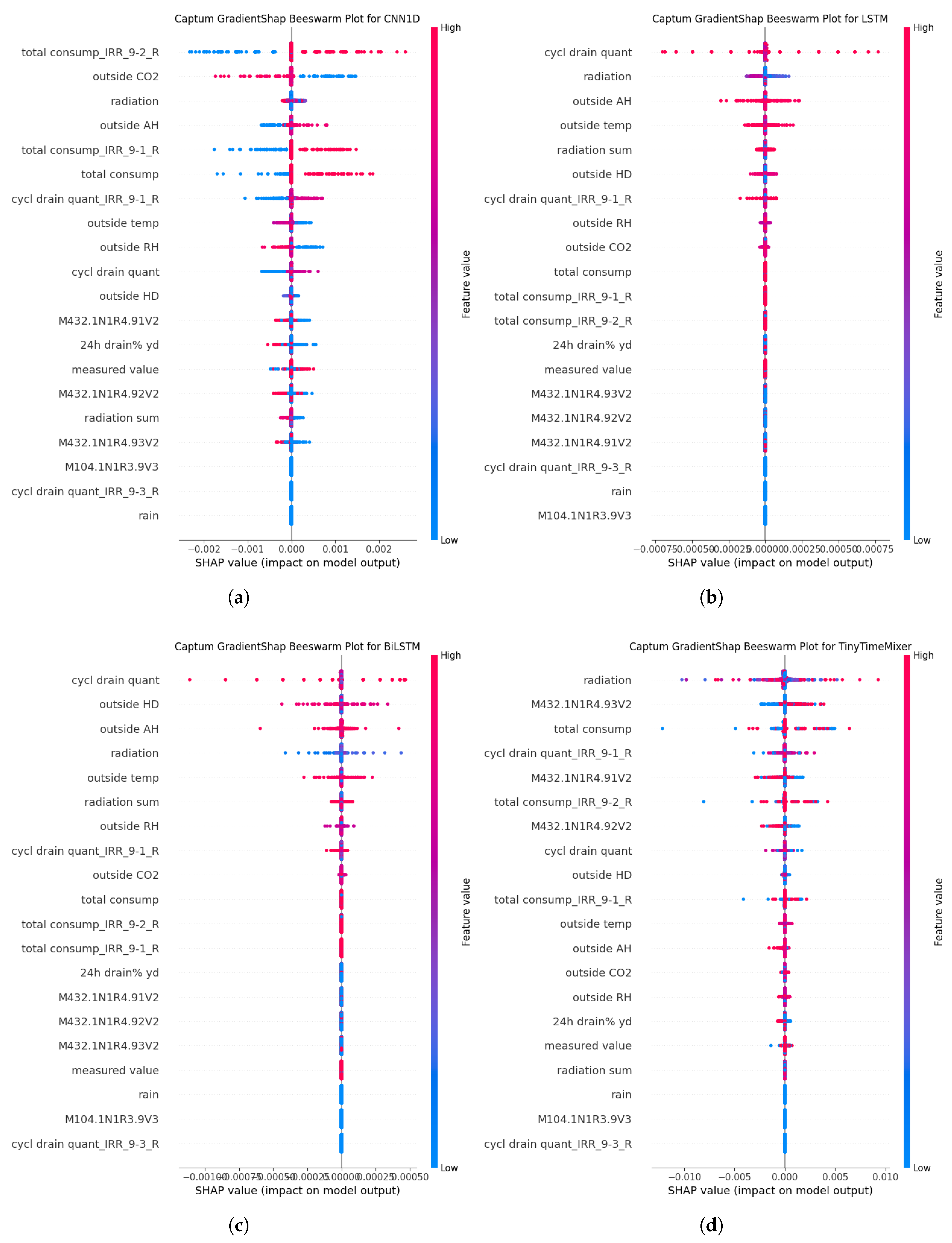
Figure 6.
Explanations for time-series model performance on predicting energy usage. (a) 1D-CNN, (b) LSTM, (c) BiLSTM, (d) TTM.
Figure 6.
Explanations for time-series model performance on predicting energy usage. (a) 1D-CNN, (b) LSTM, (c) BiLSTM, (d) TTM.
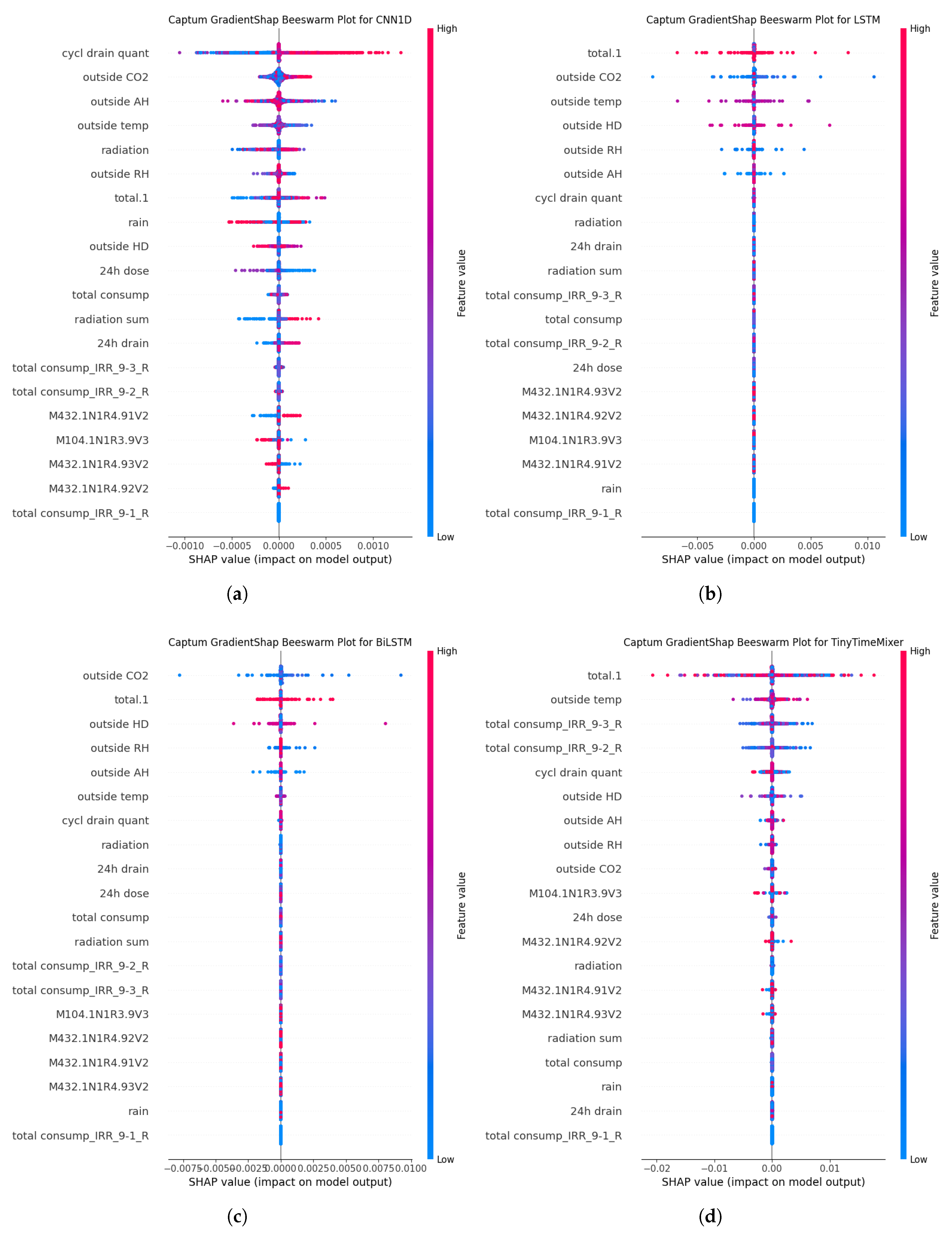
Figure 7.
TCN–CBAM explainability for Capsicum Gina: (left) feature attention weights indicating the relative importance of input variables; (right) temporal attention curve showing how the model allocates importance across the input sequence. Shaded regions denote high-attention temporal intervals, indicating periods during which climatic conditions exert a stronger influence on the prediction. Time steps (0–500) represent indexed temporal positions after alignment rather than absolute time units.
Figure 7.
TCN–CBAM explainability for Capsicum Gina: (left) feature attention weights indicating the relative importance of input variables; (right) temporal attention curve showing how the model allocates importance across the input sequence. Shaded regions denote high-attention temporal intervals, indicating periods during which climatic conditions exert a stronger influence on the prediction. Time steps (0–500) represent indexed temporal positions after alignment rather than absolute time units.
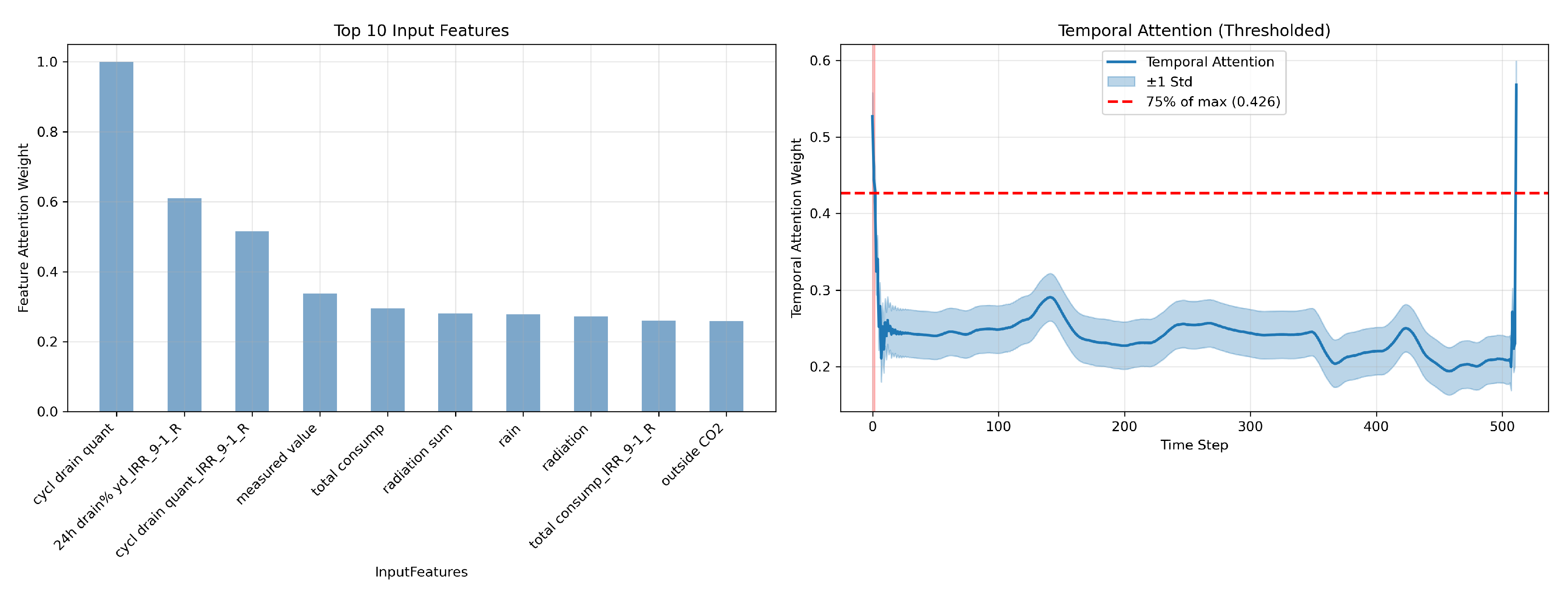
Figure 8.
TCN–CBAM explainability for energy usage: (left) top input-feature attention weights; (right) temporal attention curve with high-importance regions highlighted.
Figure 8.
TCN–CBAM explainability for energy usage: (left) top input-feature attention weights; (right) temporal attention curve with high-importance regions highlighted.
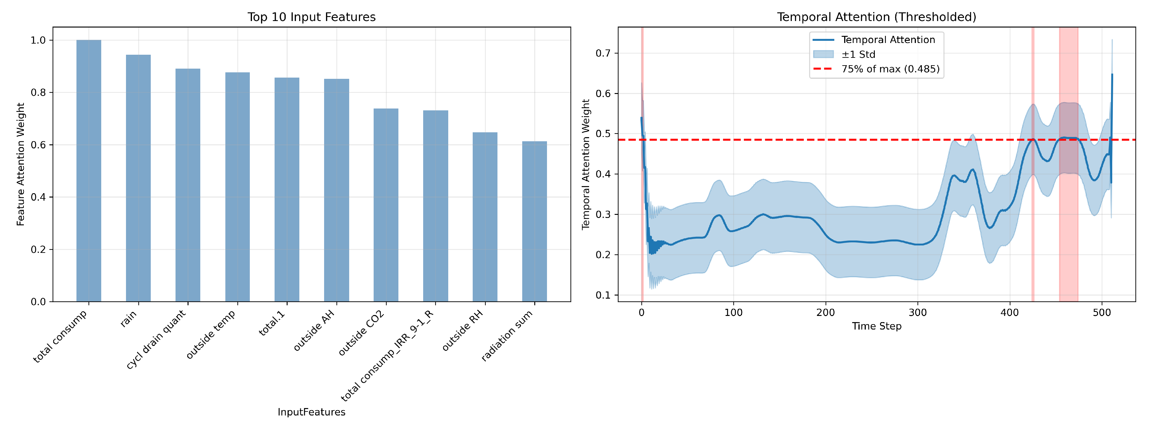
Table 1.
Comparison of time-series prediction performance across models, measured by Root Mean Squared Error (RMSE) and . The best-performing model is highlighted in bold.
Table 1.
Comparison of time-series prediction performance across models, measured by Root Mean Squared Error (RMSE) and . The best-performing model is highlighted in bold.
| 1DCNN | LSTM | BiLSTM | TTM | |||
| Capsicum | Gina | RMSE | 0.091 | 0.089 | 0.096 | 0.121 |
| 0.9841 | 0.9849 | 0.9824 | 0.9722 | |||
| YO8366 | RMSE | 0.151 | 0.156 | 0.162 | 0.193 | |
| 0.9577 | 0.9547 | 0.9515 | 0.9312 | |||
| Usage | RMSE | 0.861 | 0.690 | 0.639 | 0.254 | |
| 0.1792 | 0.4717 | 0.5475 | 0.9288 | |||
Disclaimer/Publisher’s Note: The statements, opinions and data contained in all publications are solely those of the individual author(s) and contributor(s) and not of MDPI and/or the editor(s). MDPI and/or the editor(s) disclaim responsibility for any injury to people or property resulting from any ideas, methods, instructions or products referred to in the content. |
© 2026 by the authors. Licensee MDPI, Basel, Switzerland. This article is an open access article distributed under the terms and conditions of the Creative Commons Attribution (CC BY) license (http://creativecommons.org/licenses/by/4.0/).
Copyright: This open access article is published under a Creative Commons CC BY 4.0 license, which permit the free download, distribution, and reuse, provided that the author and preprint are cited in any reuse.