
Submitted:
13 February 2026
Posted:
14 February 2026
You are already at the latest version
Abstract
Air Quality (AQ) plays a critical role in public health and urban sustainability, but drawing insights from Air Quality data remains challenging due to fragmented sources, inconsistent formats and varying measurement standards and devices. This paper explores the architecture and standardization of Air Quality datasets from major global monitoring systems, specifically the U.S. EPA’s Air Quality System (AQS) and European Environment Agency (EEA) networks, emphasizing discrepancies in pollutant units, reporting frequencies and metadata quality. The report outlines key pollutants due to road transport emissions and how they are measured using a range of technologies, from fixed regulatory stations to low-cost and satellite-based sensors. The inconsistency in schema design and the lack of interoperability across datasets hinder the scalability of machine learning (ML) pipelines, which rely on clean and harmonized inputs. To address this, an application named “Data Manager Tool” is introduced that ingests, transforms and standardizes heterogeneous AQ data into a centralized “PostgreSQL” database using a star schema. This allows more efficient querying, integration and modeling. The report discusses practical applications of this system, and how it paves the way for scalable ML-based analysis of pollution trends. Future efforts will focus on professional ML approaches, integration of mobile sensor data, and extending the framework to support predictive models and optimization using meteorological and transport datasets.
Keywords:
air quality datasets
; data preprocessing
; air quality data integration
; data standardization
; air quality digital twin
; data manager tool
1. Introduction
Air Quality monitoring is carried out by organized networks of stations and sensors which are constantly measuring pollutant concentrations in ambient air. Generally, these networks are operated by the governmental agencies, such as U.S. Environmental Protection Agency (EPA) [1], European environment agencies [2] or UK Department for Environment, Food & Rural Affairs (DEFRA) [3]. There are important missions that these networks are serving for such as, providing the up-to-date data to public, verifying compliance with Air Quality standards, trigger alerts for emergency situations, tracking the long-term trends and supply data for research, modeling and analysis. To achieve these goals successfully the regulatory frameworks like U.S Clear Air Act or the EU Ambient Air Quality Directives, mandate systematic monitoring of key pollutants at representative locations such as urban, suburban and rural sites, which determines the level of road transport emissions.
Many pollutants are regularly measured by the EEA, EPA and other institutions, the most common include PM2.5, PM10, NOₓ, CO, SOₓ, O₃ and Pb all known for their significant health impacts and commonly reported in Air Quality datasets. In addition to these, other gaseous pollutants such as carbon dioxide (CO₂), ammonia (NH₃), volatile organic compounds (VOCs), methane (CH₄), and non-methane hydrocarbons are also monitored, particularly in areas concerned with industrial emissions, climate impact, or indoor Air Quality.
The number of datasets in each region depends on the distribution of measurement stations, which are relatively sparse — typically one per several square kilometers in cities and one per tens of kilometers in rural areas. These records are usually reported as hourly or daily averages; however, the sampling interval can vary from every 10 seconds to once per hour. A typical classification of measurement areas is shown in Figure 1.
The monitoring stations are equipped with reference-grade instruments to measure pollutants like PMs, NOx, CO and SOx, often along with some metrological parameters. Data from these stations typically reported as hourly concentration values, however it can be reported more frequently as some measurement systems are able to take samples every 10 seconds and analyze it. Generally, these values get aggregated into daily, monthly or annual statistics for regulatory assessments. In the United States, for example, the EPA’s Air Quality System (AQS) serves as a central repository that stores ambient pollutant data from “over thousands of monitors”, along with meteorological readings and detailed metadata about each station’s location, operator and quality control information [4]. Similarly in Europe a system called Air Quality e-reporting system [5] (formerly AirBase) is enabling public access to Air Quality information from hundreds of stations across Europe. This system has been built on an idea of European Environment Agency (EEA) [2] for a continental data exchange where EU member states report their measurements to a centralized database. It is important to mention UK DEFRA is part of EEA’s community and is an active participant to the data exchange [6]. Figure 2 shows the overall data flow of a monitoring system.
Despite all these governmentally controlled networks, prior to recent open-data initiatives the availability of data to researchers was not straightforward. Data often resided in disparate silos managed by local agencies, and it was only accessible through annual reports. Due to the expansion of web environment and open government data policies in the last 15 years, data accessibility has greatly improved. Many agencies now publish raw monitoring data through online portals or APIs. Nonetheless, differences in data formats, units, and conventions persist across jurisdictions, necessitating careful pre-processing before such data can be merged or compared. The following sections delve into how the measurement systems work, the importance of these data for research, and a detailed review of literature on past standardization efforts and current challenges.
The importance of data for any research is evident, in this area, robust datasets enable researchers to quantify human exposure to pollutants and identify pollution sources and potentially develop predictive models. standardized Air Quality data support a wide array of applications such as scientific analysis and technological innovation. The presence of standardized datasets encourages the development of new tools like analytical software, that utilize Air Quality data.
The focus is on how data systems can be optimized, especially through standardization to maximize these benefits and what challenges remain in making Air Quality datasets compatible with “FAIR” (Findable, Accessible, Interoperable, Reusable) data principles for advanced applications like machine learning.
Studying about Air Quality trends specially with the use of AI and Machine Learning technics for prediction and analysis is an emerging area. Early studies in Air Quality often focused on developing predictive models for individual cities or pollutants, but they frequently noted the difficulties in data preparation specially in obtaining, cleaning, and combining datasets from various sources [7]. A recent study emphasizes that environmental data are interdisciplinary and that researchers may overlook critical issues in data preparation, such as handling missing data, aligning different data sources and feature engineering [8].
One of the ongoing research projects that is focused on Air Quality due to road transport emissions is the AQDT project, run by Loughborough University and supported by ARAMCO. AQDT stands for Air Quality Digital Twin, and accessible standardized air quality data is crucial for the digital twin that is being developed.
The next section of this paper focuses on the data structures and monitoring systems, followed by the currently available datasets internationally, data gathering and integration and a tool for data standardization is presented, which shows how different datasets can be normalized for comparison and model development.
2. Data Standardization in Environmental Monitoring
The European enacted INSPIRE directive required EU members to use a common data reporting model for sharing environmental information, such as Air Quality measurements [9]. As a result, Air Quality reports in Europe follows a schema with defined XML formats for hourly observations, station meta data and all other factors. This means that for instance a CO2 reading from France and one other from Italy are reported with same data fields and units under INSPIRE guidelines. While this system improved consistency for the regulatory data submitted to the EEA, it primarily covers official monitoring networks and is not being applied to the data reported from research campaigns or local low-cost sensor projects like the current Zephyr measurement system installed on Loughborough University campus. On the other hand, from the technical standard side, the Open Geospatial Consortium (OGC) has introduced a package of standards under the Sensor Web Enablement initiatives that directly address sensor data interoperability. One of the most important standards is the OGC SensorThings API, which is an open, RESTful API for the IOT sensor observations. This SensorThings API defines a consistent data model and interface for managing observations. In essence, it treats each measurement as an “Observation” linked to a “Sensor” which is the device, a “Thing” which is station hosting the sensor, a “Location” and an “ObservedProperty” which is the pollutant measured [10].
Generally, in this area the Air Quality e-Reporting framework which extends INSPIRE, is a good example. It not only standardizes format but also automates data submission from national databases to the EEA. Through this system, hourly data from over 4,000 stations across Europe are fed into a central repository and made available via download services. This represents a continent-scale implementation of standardized data collection. Likewise, the U.S. EPA has modernized its Air Quality System by offering a public API (the AQS Data Mart API) that serves data in a consistent CSV/JSON structure, and by adopting common coding for pollutants, units and station metadata nationwide. However, the AQS reporting system is only offering daily reports via downloadable files or through APIs.
Despite all these efforts, still for a research project which leverages ML techniques for its analysis, there are many obstacles in data gathering and integration. Particularly due to different reporting formats such as Parquet files for EU EEA and CSV/JSON files for US AQS and inconsistent reporting timestamps like hourly reports for EU EEA and daily reports for US AQS as well as different measurement units such as µg/m3 for EU and ppb for US, this is evident that there is no pre built interface which can get integrated to these ends and by processing the data makes a robust database. Figure 3 contains two screenshots from the reports provided by EU EEA and U.S EPA as two examples.
The FAIR data principles have been defined in 2016 by Mark D. Wilkinson et al., and its name stands for Findability, Accessibility, Interoperability and Reusability. Later in 2019 the follow-up addendum clarifies that a dataset is in accordance with FAIR while it is metadata complete and machine readable. These principles are essential in environmental informatics, where heterogeneous observational sources complicate seamless reuse [11,12].
3. Air Quality Monitoring Systems
There are several Air Quality measurement systems working across the globe, some are connected and centralized networks such as EEA in Europe or EPA AQS in United States. These networks are having both spatial and temporal sensors with different specifications. For instance, the frequency of sampling or reporting values aggregation varies in each specific station but generally, typical pollutants and parameters measured and reported. Air Quality measurement systems are fundamental to monitoring atmospheric conditions and understanding pollution patterns. These systems encompass a wide array of technologies, from ground-based regulatory stations to satellite instruments, each with specific roles, spatial and temporal resolutions, and operational protocols. Their integration enables comprehensive assessment of air pollutants, supporting both scientific research and regulatory compliance. Figure 4 shows different types of measuring systems.
The Fixed Regulatory Monitoring Stations utilize a range of scientifically validated measurement methods, including automatic analyzers, active sampling and passive sampling to monitor key atmospheric pollutants—such as particulate matter (PM2.5 and PM10), nitrogen dioxide (NO₂), Sulphur dioxide (SO₂) and ozone (O₃). For most of the pollutants, monitoring stations must fulfil the criterion of reporting more than 75% of valid data out of all the possible data in a year [13,14].
One of the most common instruments used for measuring particulate matter (PM2.5 and PM10) is the Beta Attenuation Monitor (BAM). The BAM technique relies on the attenuation of beta radiation as it passes through a filter tape on which ambient particulate matter has been collected. Specifically, a small carbon-14 or krypton-85 radioactive source emits beta particles that are absorbed proportionally by the mass of particles on the filter. The reduction in beta particle count is measured on the other side of the tape by a Geiger-Müller detector, and this attenuation is directly correlated to the mass concentration of the particles [15]. For gaseous pollutants such as NO₂, chemiluminescence detection is considered the gold standard. This technique involves a gas-phase reaction between NO and O₃, which produces electronically excited nitrogen dioxide (NO₂). As NO₂ returns to its ground state, it emits light in the near-ultraviolet region. The emitted light intensity is proportional to the NO concentration in the air sample. To measure total NOₓ (NO + NO₂), the sample stream passes through a converter that reduces NO₂ to NO, thereby enabling indirect measurement of both components [16]. Ozone concentrations are commonly determined using UV photometry, which leverages the strong ultraviolet absorption characteristics of ozone at 254 nm. A UV lamp emits radiation through a sample cell containing ambient air, and a photodetector on the opposite side measures the transmitted light. The attenuation of the light intensity, calculated using Beer-Lambert’s Law, provides a direct measure of the ozone concentration [17]. Carbon monoxide (CO) levels are measured using non-dispersive infrared (NDIR) spectroscopy, which detects the specific absorption of infrared radiation by CO molecules. An IR source emits radiation through a gas sample, and the degree of IR absorption is recorded by a detector. The extent of absorption, interpreted via Beer’s Law, provides a quantitative measure of the CO concentration [18]. To contextualize Air Quality measurements, the physical location of each station is categorized based on surrounding land use and population density into urban, suburban, or rural classifications. This spatial classification helps characterize local emissions and pollution sources as well as atmospheric transport patterns. The density and distribution of buildings around each station are taken into account in determining this classification. Moreover, many stations are co-located with meteorological sensors such as anemometers, thermometers, and hygrometers. These sensors are crucial for interpreting pollutant dispersion, atmospheric chemical transformations, and boundary layer processes [19]. Data quality is ensured through comprehensive Quality Assurance/Quality Control (QA/QC) procedures, including regular calibration with certified gas standards, instrument audits, and preventive maintenance. These methods maintain the scientific integrity and regulatory reliability of fixed monitoring networks, which remain essential for comprehending and managing ambient Air Quality.
The Low-Cost Sensors: Recently, these sensors have received considerable attention due to their affordability, compact design, and appropriateness for dense spatial deployment, especially in urban areas and regions deficient in regulatory monitoring infrastructure. These sensors typically utilize fundamental physical and chemical detecting principles, sacrificing a measure of precision for low power consumption, compactness, and cost efficiency. Despite these limitations, when appropriately calibrated and quality-controlled, low-cost sensors provide significant insights into air pollution dynamics, especially for public engagement and supplementary research purposes. Their successful application relies on comprehension of the fundamental measurement principles—such as light scattering, electrochemical reactions, and semiconductor sensing—alongside meticulous deployment, validation, and data processing. Low-cost sensors for particulate matter (PM2.5 and PM10) often utilize light scattering methods, particularly optical particle counters (OPCs).). These devices operate based on Mie scattering theory, which describes how particles scatter light when illuminated by a source, often a laser diode. As particles pass through the sensing chamber, they scatter light, which is then detected by a photodiode or photomultiplier tube. The scattered light intensity is used to infer particle size and concentration. Mass concentrations are estimated through calibration with reference-grade instruments or using standard aerosols [20]. For measuring gaseous pollutants such as NO₂, O₃, and CO, electrochemical sensors are most commonly used. These consist of electrodes immersed in an electrolyte and enclosed in a gas-permeable membrane. Target gases diffuse through the membrane and undergo redox reactions at the electrodes, producing an electric current proportional to gas concentration. The measured current is governed by Faraday’s laws of electrolysis. However, these sensors are sensitive to temperature and humidity variations, necessitating correction algorithms to improve accuracy [21]. In addition, metal oxide semiconductor (MOS) sensors are used for certain oxidizing gases, particularly ozone. These sensors incorporate materials such as tin dioxide (SnO₂), whose electrical resistance varies in response to gas interactions at the surface. Changes in resistance are interpreted as variations in gas concentration, although these sensors often suffer from limited selectivity and cross-sensitivity to other atmospheric compounds and environmental parameters [22]. While these sensor technologies provide advantages such as portability, real-time data, and low deployment costs, their effectiveness relies heavily on rigorous calibration protocols. Co-location with reference instruments is a key step in identifying and correcting for biases, sensor drift, and cross-interference. Calibration methods range from basic linear regression to more sophisticated machine learning algorithms that account for meteorological conditions and sensor aging [23]. Networks such as PurpleAir, Sensor Community, and AirQo have demonstrated the potential of distributed low-cost sensor systems to enhance public engagement, supplement traditional monitoring efforts, and inform environmental policy. However, the interpretability and utility of data from these networks are contingent on robust calibration practices and context-aware data analysis [23] Although low-cost sensors are not yet substitutes for regulatory-grade instruments, they are playing an increasingly important role in expanding the spatial reach of Air Quality monitoring.
The Remote Sensing (Satellite-Based Measurements) data complement ground-based measurements, providing broader spatial coverage and aiding in identifying pollution trends, The EEA utilizes data from satellite instruments like the Ozone Monitoring Instrument (OMI) to assess pollutants such as O3, NO2, and SO2. In North America, The EPA collaborates with NASA on satellite missions like the Tropospheric Emissions: Monitoring of Pollution (TEMPO) instrument, which measures air pollutants with a high resolution and on an hourly basis [24]. Satellite-based remote sensing plays a vital role in global and regional Air Quality monitoring by providing consistent, large-scale observations of atmospheric constituents. The core principle behind satellite measurements of air pollutants is the interaction between solar radiation and atmospheric gases, which results in absorption or scattering of light at specific wavelengths. By measuring the intensity of reflected or transmitted light across different spectral bands, satellites can infer the presence and concentration of pollutants such as NO2, SO2, O3, CO, and aerosols. Most satellite instruments operate based on passive remote sensing, utilizing sunlight as an illumination source. Instruments like the Ozone Monitoring Instrument (OMI) aboard NASA’s Aura satellite and TROPOspheric Monitoring Instrument (TROPOMI) onboard Sentinel-5P are hyperspectral spectrometers that measure the backscattered solar radiation from the Earth’s atmosphere and surface across ultraviolet, visible, and near-infrared bands. These measurements are interpreted using Beer-Lambert’s Law, which relates the attenuation of light at specific wavelengths to the concentration of absorbing species in the atmospheric column [25,26]. For example, NO2 has strong absorption features in the ultraviolet-visible spectrum (350–450 nm). By quantifying the differential absorption at these wavelengths, the total vertical column density (VCD) of NO2 can be derived. However, satellites typically measure slant column densities (SCDs)—the integrated concentration along the optical path. These are then converted to VCDs using air mass factors (AODs), which account for solar zenith angle, surface reflectivity (albedo), aerosol loading, and vertical profile shape [27]. To estimate surface-level concentrations from column measurements, satellite data are often combined with chemical transport models (CTMs) such as GEOS-Chem or CMAQ. These models incorporate meteorological inputs and emissions inventories to simulate the vertical distribution of pollutants, thereby facilitating the estimation of surface concentrations through vertical profile shaping and data assimilation techniques [28]. Recent advancements include the TEMPO instrument, which operates in geostationary orbit, allowing for continuous, high-temporal-resolution measurements over North America. TEMPO employs high-resolution spectrometry in the ultraviolet and visible ranges to capture hourly variations in NO2, O3, SO2, and formaldehyde [29]. Unlike sun-synchronous polar orbiters, geostationary sensors provide improved diurnal coverage, essential for studying short-term emissions events and atmospheric chemistry. In addition, some satellite systems use active remote sensing techniques, such as Light Detection and Ranging (LIDAR). These instruments emit laser pulses and measure the backscattered return signal to obtain vertically resolved profiles of aerosols and, in some cases, trace gases. While less common in operational satellite platforms, LIDAR systems offer valuable insights into the vertical structure of the atmosphere. The physical principles behind satellite remote sensing of Air Quality is governed by radiative transfer theory, molecular absorption cross-sections, and atmospheric scattering processes. These observations are indispensable for monitoring long-range pollutant transport, evaluating emission inventories, validating Air Quality models, and supporting environmental policy. The TEMPO mission represents a major step forward in our ability to observe atmospheric composition at fine temporal and spatial scales, enhancing our understanding of pollutant sources, distributions, and their evolution over time [28].
Supporting Measurements: Air Quality stations often include meteorological sensors (temperature, humidity, wind speed/direction) because weather conditions strongly influence pollution levels. Some networks measure additional parameters like volatile organic compounds (VOCs), ammonia, or greenhouse gases, depending on objectives. For Machine Learning, having these auxiliary variables can be valuable as features.
The integration of ground-based and satellite Air Quality monitoring systems is crucial for obtaining accurate, spatially detailed, and temporally uniform evaluations of atmospheric pollution. Each of these platforms offers unique strengths and limitations: ground-based stations provide high-accuracy time series data but are spatially sparse; satellites provide global coverage but suffer from coarse resolution and limited surface sensitivity. Researchers utilize a blend of calibration frameworks, statistical data fusion, and chemical transport modeling to integrate data from these diverse sources [23,28]. At the foundational level, calibration against ground-based regulatory stations is central to aligning measurements across platforms. Ground stations—equipped with reference-grade instruments—serve as the gold standard, enabling calibration of low-cost sensor networks through co-location experiments. Correction models are built during calibration campaigns to address sensor drift, environmental dependencies (e.g., temperature, humidity), and cross-sensitivity to non-target gases. Techniques vary from simple linear regressions to complex machine learning algorithms such as random forests and neural networks [23].
For satellite observations, which generally provide total column densities of trace gases (e.g., NO₂, SO₂, O₃), depend on the calibration and interpretation through the integration of radiative transfer models and CTMs. These models integrate real-world meteorological fields and emissions inventories to simulate the vertical profiles of pollutants, which are essential for estimating near-surface concentrations relevant to human exposure. Ground-based measurements are used to validate and bias-correct these modelled profiles, thereby closing the loop between in situ and remotely sensed observations [28].
Data fusion techniques play a critical role in integrating observations across networks. Approaches such as spatiotemporal kriging, Bayesian hierarchical models, and geostatistical smoothing are commonly used to interpolate pollutant fields by combining satellite, ground-based, and data. More advanced systems employ data assimilation techniques—including variational methods (3D-VAR, 4D-VAR) and ensemble Kalman filters—to iteratively adjust CTM outputs using real-time observational data. These assimilation techniques enhance model realism and provide improved estimates of pollutant distributions, particularly in data-sparse regions.
Global efforts to operationalize such integrated frameworks have led to the development of platforms like CAMS (Copernicus Atmosphere Monitoring Service) and NASA’s MAIAC algorithm, which systematically combine satellite aerosol optical depth (AOD) with surface PM2.5 measurements [28]. Similarly, OpenAQ and Google Air View use calibrated low-cost sensors to complement official monitoring networks and provide hyperlocal pollution mapping [30]. These integrative approaches reflect a paradigm shift in Air Quality science—from single-source monitoring to multi-platform, model-assisted observation systems—enabling comprehensive air pollution assessment at scales relevant to policy, health, and climate research.
4. Available Datasets
There is a need for a standardized dataset containing global Air Quality records for future research. The data from different sources lack consistency in terms of time frames and the pollutants being monitored, for instance, some areas focus mainly on NO and CO levels, while others also measure O₃, PM₁₀, and PM₂.₅ or others.
Additionally, there are some Air Quality data sources that are not publicly accessible, such as data from the Earth Sense portal, which collects measurements from devices installed on the Loughborough University campus and in other areas. The Zephyr devices are taking samples every 10 seconds, and “My Air” platform processes the data, providing averaged results over periods ranging from 5 minutes to 24 hours.
A wide number of Air Quality datasets are published under open and permissive licensing frameworks; however, the specifics vary by source and jurisdiction. As an example, the US EPA’s Air Quality system AQS data is openly accessible through downloadable files and APIs. In Europe, data portals like data.europa.eu default to open licensing, often under CC-BY-4.0, though individual datasets carry dataset-specific terms. Overall, while accessibility is generally high via direct downloads or APIs, the exact legal reuse conditions vary and must be verified per dataset. Additionally, OpenAQ, a nonprofit initiative, emphasizes “universal access” to Air Quality measurements, enabling comprehensive reuse, but similarly lacks detailed license documentation.
Metadata quality across Air Quality repositories differs widely, influencing usability and interoperability. EPA’s AQS includes detailed metadata accompanying datasets such as instrument type, geolocation and pollutant parameters. Users can also access data via OData for seamless integration. Similarly, World Health Organization (WHO) database provides metadata on pollutant types, urban context, data sources and compilation date, but metadata richness can vary depending on national source contributions. European portals also adopt rich metadata standards furnishing multilingual descriptions, data provenance and license information. In summary while government and research data often include robust metadata, completeness still varies especially in crowd sourced platforms and global aggregators necessitating careful review for each dataset.
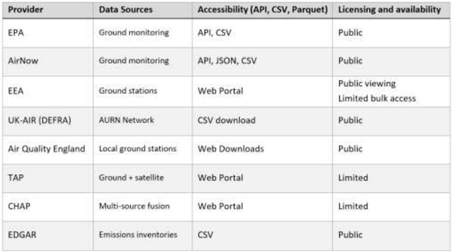
Several publicly accessible datasets provide reliable and regularly updated Air Quality information across different regions of the world. Notable examples include have been included in Table 1:
1. EPA - Air Quality Index (AQI) Daily Values Report [31] (USA): A national level dataset offering daily and hourly (for some pollutants) records of AQI and pollutant concentrations for locations across the United States. This data is published by the EPA and is reported per monitoring station and can be aggregated by county or Core-Based Statistical Area (CBSA).
2. AirNow Developer Tools [32]: EPA is collaborating with another organization called AirNow, this platform is providing forecast and real-time observed Air Quality information across the United States, Canada, and Mexico. AirNow receives real-time Air Quality observations from over 2,000 monitoring stations and collects forecasts for more than 300 cities.
3. European Air Quality Index (EAQI) [33]: Coordinated by the EEA, this index consolidates Air Quality data from across Europe and standardizes it for comparability and public accessibility, generally the measured factors are NO2, PM10 and PM2.5. The index uses data from over 1,000 monitoring stations, with a spatial resolution of approximately 10 km x 10 km [34].
4. UK-AIR - Daily Air Quality Index (UK) [35]: Managed by the UK DEFRA, this dataset provides daily Air Quality levels and health-based categorizations across the UK. UK-AIR data is collected from the Automatic Urban and Rural Network (AURN), with each monitoring station representing its immediate area [36]. There are 194 working stations (as of May 2025) and the recorded data is available from early 1970s up to now.
5. Air Quality England (AQE) [37]: A network of monitoring stations across England providing localized, near real-time Air Quality data and historical records. AQE data is updated hourly for NO2 and NO and for PM10 and PM2.5 data is getting updated in daily basis. The monitoring stations are typically placed in urban areas, with each station representing local conditions [36].
6. Tracking Air Pollution (TAP) in China: A high-resolution Air Quality dataset focusing on PM2.5 concentrations across China, integrating ground measurements, satellite observations, and predictive modeling.
7. China High Air Pollutants (CHAP): This resource offers a long-term, full-coverage and high-resolution record of ground-level air pollutants across mainland China developed using a fusion of ground-based station measurements, satellite remote sensing, atmospheric reanalysis and model simulations. It covers all main pollutants and even includes chemical composition of PM₂.₅ (e.g., SO₄²⁻, NO₃⁻, NH₄⁺, Cl⁻, BC, OM) and polycyclic aromatic hydrocarbons (PAHs). The dataset enables high-spatial-resolution (1 km) and daily, monthly or annual analyses across all of China, making it well suited for trend analysis, exposure assessment, policy evaluation and spatial modeling of Air Quality [38,39].
8. Emissions Database for Global Atmospheric Research (EDGAR): This global dataset, developed by the European Commission’s JRC, offers comprehensive estimates of greenhouse gas and air pollutant emissions from human activities across all countries. EDGAR provides detailed emission data for pollutants, categorized by sector and country. The database includes annual time series and high-resolution spatial grid maps, facilitating analysis of emission trends and spatial distribution, while annual data is standard, some datasets offer monthly and hourly temporal profile. Emissions data is provided at a global scale with a spatial resolution of 10km x 10km. EDGAR’s data supports climate policy development, Air Quality management, and scientific research by providing consistent and comparable emission inventories worldwide.
5. Data Structures, Gathering and Integration
Air Quality datasets come in a variety of data structures, and this structural difference is more than cosmetics, it affects how easily data from different sources can be combined and fed into the machine learning pipelines. A few common patterns and their associated challenges are discussed below:
Wide Schema Representations: One common format for historical Air Quality datasets is a “wide” table schema, where each monitoring site has a separate file or table, and each pollutant is a column in that table, with rows indexed by time (see Figure 3).
For example, a city might provide a CSV file for station X containing columns like: Date, PM₁₀, PM₂.₅, NO₂, O₃, etc., all in one sheet. This is convenient for looking at one station’s multi-pollutant profile but becomes weighty when integrating many stations or doing pollutant-centric analysis. Additionally, in a wide schema, if one station doesn’t measure a particular pollutant, it might use a placeholder (NA) or exclude that column, leading to inconsistent columns across stations.
Variability Across Datasets (Units, Timestamps): As introduced, units are a big variability point. For instance, 1 ppb of gas X has a different µg/m³ value. Many European datasets stick to µg/m³ for everything (for regulatory consistency), whereas US datasets use ppb for gases. This means any integrated dataset must choose a unit convention and convert all sources accordingly.
All these inconsistencies mean that a considerable pre-processing stage is required before data can be fed to ML models a suitable data set should have:
- Normalized units, introducing potential conversion errors if done incorrectly.
- Aligned time bases, ensuring each record’s timestamp is comparable.
- Appropriate handling techniques to mitigate the impact of missing data.
- Merge data from multiple stations or sources often involving pivoting between wide and long formats.
Machine Learning pipelines typically prefer a long-normalized format, each row is one observation of one pollutant at a time and location with columns for station id, time, pollutant value, etc. This is more database-like. Interestingly, many official databases like the EEA’s internal SQL, and the EPA’s AQS do store data in such a long format internally, but when exporting to users they convert it to a more human consumable wide format or CSVs separated by pollutant.
The Air Quality data is getting measured and stored by different institutions across the world, this fact makes the data gathering complicated. The complication is mainly because of the data structure and technical filing or integration formats. Generally, institutions like EPA and EEA, are offering both file exports and APIs which have their own complexities and specification. In this research project, the aim is to being able to collect data from different end points, thus, a robust toll called data manager tool is overseeing this process. In the file interpretation section, the system can get CSV files, standardize them and pass the data in the correct format to the centralized database. The point about this feature is that the system needs to be tuned for each institutions reporting format and once the algorithm can detect the source of the uploading dataset can standardize the data accordingly. In contrast, the system has another feature which works directly with the Air Quality data end points. This process can be done automatically using the automation or manually by the request of clients. The process of data ingestion requires certain factors to be passed to the main backend algorithm, such as, geographic location information (longitude and latitude), the start and end time of the period being queried in Unix time format, and if the ingestion request is made manually by a client, a name to be defined for that exact location, which helps avoid data duplication and related issues in the future. If this microservice is integrated into a larger system and called continuously by other orchestration mechanisms, these requirements must be addressed from the very first attempt.
One of the optimized ways to have control over time-dependent events in computers is to leverage Unix time in the algorithm. This number is a continuous monotonically, incremental integer, which reduces the possibility of making mistakes when dealing with time in computers. The backend algorithm could convert and store the data coming with usual date time formats and store them with Unix time timestamps. This scenario mostly happens when the input is CSV formatted datasets and added manually or the system is getting integrated into another service which works with general date time formats.
There are other pre-processing steps that need to be taken to create a standardized dataset and prepare the ground for ML algorithms. For example, the algorithm should be able to recognize, and report missing values in the reports and handle daily measured datasets in the same way as hourly averages. This is important because the number of cells in the dataset should remain consistent, for instance, when uploading a daily reported dataset for standardization and clustering, the algorithm will replicate the reported value 24 times to represent each hour of that day for the specified location.
To ensure a standardized data source for machine learning applications, it is important to have a database with a consistent clustering format and schema. In our example for storing Air Quality data, employing a star schema within a PostgreSQL database is an optimized solution. Considering the nature of Air Quality data, key tables are locations, metrics and parameters (Figure 5). Each location (having longitude and latitude) is assigned a unique identifier which acts as a primary key and links to the corresponding metrics for that specific geographical area. The metrics table records measurements for each location over defined time intervals, typically on an hourly basis, reflecting the standard temporal resolution of Air Quality reports. Air Quality information such as, specific parameter values and meteorological data are stored in separate tables and linked to the metrics table via foreign key relationships. Thus, the parameters table contains individual entries representing the recorded values of various Air Quality and meteorological variables for a given location and time.
6. Tool Development for Standardization
As a microservice of a whole system, the data gathering and providing service will be handled by the Data Manager Tool (Figure 6). In this project a Python Starlette layer oversees all backend handling systems, it has been chosen because of its robustness and agility in handling APIs. Thus, Data Manager Tool’s duty in this project, is to get integrated with Air Quality data providers such as OpenWeatherMap using APIs, and to get integrated to the Air Quality Digital Twin (AQDT) custom interface to be able to inject manually reported Air Quality data to the database in a standard format and finally provide REST APIs for the machine learning purposes.
Two data pipelines are used to supply raw Air Quality data to the Data Manager Tool. The first pipeline relies on automated data acquisition through application programming interfaces (APIs), while the second involves the manual upload of Air Quality datasets such as CSV files via the system interface. For API-based integrations, several public data providers worldwide offer Air Quality services, including the EEA in Europe and the EPA in the United States. In addition to these public sources, private institutions also provide Air Quality APIs, such as OpenWeatherMap [40], which offers a robust and widely used service. Figure 7 illustrates an example of an API request and its corresponding JSON response from this provider.
One of the most important advantages of OpenWeatherMap services is that they offer historical meteorological data of each geographic location as well as the Air Quality data, measured by the satellite systems. This is an opportunity to get all the required information from one end, which lowers the calibration and technical complexities. On the other hand, an interface has been designed to be able to get the raw Air Quality data files in CSV format from the clients to standardize and store them into the database for machine learning purposes. In this process, getting daily and hourly measured reports was a challenge and to avoid having recorded data with different temporal resolution, one of the initiatives was to record each daily report as a 24-hourly reported metrics, however, there are more sophisticated techniques that could be used in the future.
For having an agile data management system, automation is a crucial part of the whole system. Nowadays, due to the advancement of technology, especially in data integration and data pipelines, there are many ways to make the different components of a system integrated. Additionally, for a more sophisticated system like a digital twin, one of the most important attributes is its robustness in terms of the ability of near real time integration within all system components. Thus, automation is central to ensuring the AQDT operates with minimal intervention while maintaining data accuracy and timeliness. The data manager tool automates ingestion from multiple APIs such as the OpenWeatherMap as well as manual uploads, adapting to differences in formats, units and temporal resolutions through scheduled jobs and queued tasks. Data is retrieved, validated, harmonized and stored in the PostgreSQL star schema without manual reconfiguration. The harmonization stage standardizes units, aligns timestamps and resolves missing values enabling downstream ML models to work with uniform high-quality inputs. For daily datasets, the system can automatically expand values to hourly resolution, ensuring schema consistency. An example of which data are ingested, standardized and stored in the database is demonstrated in a video screenshot on AQDT website [41]. Scalability is supported by partitioned tables, indexed keys and containerized API services, allowing the architecture to expand horizontally as new locations, pollutants or resolutions are added.
Having a standardized database full of Air Quality data from various resources is a step forward and has benefits for both scientific research and policy development. And for this research project, having access to harmonized data unlocks the potential of large-scale ML applications. This application also allows environmental scientists, data engineers and public health experts to work with an updated dataset that automatically fetches raw data from AQ data providers APIs. The data manager tool can provide data to authorized 3rd parties by offering secured data pipelines that leverage the OAuth 2.0 [42] protocol for authentication and access control.
The Data Manager Tool (DMT), presented by this paper, is a robust tool for making the ground ready for sophisticated Air Quality platforms. However, there are still areas for improvement, for example, the system can support integration with more Air Quality networks and ideally provide an interface capable of ingesting data from any source which can be done by applying AI techniques and it could automatically detect errors, standardize data and cluster it effectively.
7. Conclusion
One of the most persistent challenges in contemporary Air Quality research arises from the inconsistency and fragmentation of datasets across monitoring networks, institutions and regions. Researchers frequently face difficulties when attempting to merge and analyze data collected under differing formats, units of measurement and temporal resolutions. These differences are not just technical problems; they seriously affect how well studies can be compared or repeated. When data is stored in different formats, uses different units or lacks proper organization, it becomes very hard to use for advanced modeling or machine learning. Without consistent data preparation, researchers spend a great deal of time fixing and aligning datasets instead of focusing on meaningful analysis and interpretation. Differences in schema design, missing metadata and inconsistent data quality control practices further amplify these issues, often resulting in significant pre-processing burdens and methodological uncertainty. Thus, a considerable proportion of research effort is devoted not to analysis, but to data wrangling, normalization and harmonization.
The Data Manager Tool (DMT) introduced in this study directly addresses these systemic issues through a unified and scalable approach to Air Quality data integration. By employing automated ingestion pipelines, schema-based normalization and robust pre-processing logic, the DMT transforms heterogeneous datasets—originating from institutions such as the US EPA, European EEA, or local low-cost sensor networks, into a harmonized and analysis-ready structure. Its star-schema implementation within a PostgreSQL framework ensures both relational integrity and flexibility for large-scale querying, thereby enabling researchers to efficiently access multi-source Air Quality records with standardized units and aligned temporal granularity. Moreover, by automating conversion processes, handling missing data and ensuring consistent timestamping through Unix time encoding, the system minimizes manual intervention and mitigates human error.
This data harmonization framework also represents a foundational step toward the operationalization of the FAIR data principles within environmental informatics. The DMT enables Air Quality datasets to be Findable, Accessible, Interoperable, and Reusable, which is essential for scientific transparency, reproducibility and interdisciplinary collaboration. Its automation capabilities and support for both API-driven and manual data ingestion, establish the groundwork for dynamic and near-real-time integration which is an important milestone toward the creation of intelligent environmental digital twins.
Abbreviations
The following abbreviations are used in this manuscript:
| 3D-VAR | Three-dimensional variational data assimilation |
| 4D-VAR | Four-dimensional variational data assimilation |
| AAE | Aeronautical and Automotive Engineering |
| AACME | Aeronautical, Automotive, Chemical and Materials Engineering |
| AOD | Aerosol Optical Depth |
| AMF / AMFs | Air Mass Factor(s) |
| API / APIs | Application Programming Interface(s) |
| AQ | Air Quality |
| AQDT | Air Quality Digital Twin |
| AQE | Air Quality England |
| AQI | Air Quality Index |
| AQS | Air Quality System |
| AURN | Automatic Urban and Rural Network |
| BAM | Beta Attenuation Monitor |
| BC | Black Carbon |
| CBSA | Core-Based Statistical Area |
| CAMS | Copernicus Atmosphere Monitoring Service |
| CC-BY-4.0 | Creative Commons Attribution 4.0 International |
| CHAP | China High Air Pollutants |
| CH₄ | Methane |
| CLD | Chemiluminescence Detection |
| CMAQ | Community Multiscale Air Quality |
| CO | Carbon Monoxide |
| CO₂ | Carbon Dioxide |
| CPC | Condensation Particle Counter |
| CTM / CTMs | Chemical Transport Model(s) |
| CSV | Comma-Separated Values |
| DEFRA | Department for Environment, Food & Rural Affairs |
| DMT | Data Manager Tool |
| EAQI | European Air Quality Index |
| EDGAR | Emissions Database for Global Atmospheric Research |
| EEA | European Environment Agency |
| ELPI | Electrical Low Pressure Impactor |
| EMROAD | EMission model for ROAD vehicles |
| EPA | Environmental Protection Agency |
| EU | European Union |
| FAIR | Findable, Accessible, Interoperable, Reusable |
| FID | Flame Ionisation Detection |
| GEOS-Chem | GEOS-Chem |
| INSPIRE | Infrastructure for Spatial Information in Europe |
| IoT | Internet of Things |
| JRC | Joint Research Centre |
| JSON | JavaScript Object Notation |
| LIDAR | Light Detection and Ranging |
| MAIAC | Multi-Angle Implementation of Atmospheric Correction |
| MAW | Moving Average Window |
| ML | Machine Learning |
| MOS | Metal Oxide Semiconductor |
| NASA | National Aeronautics and Space Administration |
| NDIR | Non-Dispersive Infrared |
| NH₃ | Ammonia |
| NO | Nitric Oxide |
| NO₂ | Nitrogen Dioxide |
| NOₓ | Nitrogen Oxides |
| O₃ | Ozone |
| OAuth 2.0 | OAuth 2.0 |
| OData | Open Data Protocol |
| OGC | Open Geospatial Consortium |
| OMI | Ozone Monitoring Instrument |
| OM | Organic Matter |
| OPC | Optical Particle Counter |
| PAHs | Polycyclic Aromatic Hydrocarbons |
| Parquet | Parquet (columnar file format) |
| Pb | Lead |
| PEMS | Portable Emission Monitoring Systems |
| PM | Particulate Matter |
| PM₂.₅ | Particulate Matter ≤ 2.5 μm |
| PM₁₀ | Particulate Matter ≤ 10 μm |
| QA/QC | Quality Assurance / Quality Control |
| RDE | Real Driving Emissions |
| REST | Representational State Transfer |
| SCD | Slant Column Density |
| SnO₂ | Tin(IV) oxide |
| SO₂ | Sulphur Dioxide |
| SOₓ | Sulphur Oxides |
| TAP | Tracking Air Pollution |
| TEMPO | Tropospheric Emissions: Monitoring of Pollution |
| THC | Total Hydrocarbons |
| TROPOMI | Tropospheric Monitoring Instrument |
| UK-AIR | UK Air Information Resource |
| UV | Ultraviolet |
| VCD | Vertical Column Density |
| VOCs | Volatile Organic Compounds |
| WHO | World Health Organisation |
| WLTC | Worldwide Harmonized Light Vehicles Test Cycle |
| XML | eXtensible Markup Language |
References
- U.S. Environmental Protection Agency. EPA n.d. https://www.epa.gov/ (accessed 5 December 2025).
- European Environment Agency. European Environment Agency Website n.d. https://www.eea.europa.eu/en (accessed 5 December 2025).
- Department for Environment F & RA. UK AIR n.d. https://uk-air.defra.gov.uk/ (accessed 5 December 2025).
- US EPA. EPA Air Quality System (AQS) n.d. https://www.epa.gov/aqs (accessed 28 May 2025).
- European Environment Agency. E-reporting System n.d. https://www.eea.europa.eu/en/datahub/datahubitem-view/3b390c9c-f321-490a-b25a-ae93b2ed80c1https://www.eea.europa.eu/en/datahub/datahubitem-view/3b390c9c-f321-490a-b25a-ae93b2ed80c1 (accessed 5 December 2025).
- UK AIR - DEFRA. European Pollution Levels n.d. https://uk-air.defra.gov.uk/latest/european-pollution-levels (accessed 28 May 2025).
- Tang, D; Zhan, Y; Yang, F. A review of machine learning for modeling air quality: Overlooked but important issues. Atmos Res 2024, 300. [Google Scholar] [CrossRef]
- Tang, D; Zhan, Y; Yang, F. A review of machine learning for modeling air quality: Overlooked but important issues. Atmos Res 2024, 300, 107261. [Google Scholar] [CrossRef]
- European Commission. INSPIRE Directive 2007. https://knowledge-base.inspire.ec.europa.eu/legislation/inspire-directive_en.
- OGC. OGC SensorThings API for European Green Deal Data Spaces n.d. https://www.ogc.org/blog-article/ogc-sensorthings-api-for-european-green-deal-data-spaces (accessed 2 June 2025).
- Wilkinson, MD; Dumontier, M; Aalbersberg, IjJ; Appleton, G; Axton, M; Baak, A; et al. Comment: The FAIR Guiding Principles for scientific data management and stewardship. Sci Data 2016, 3. [Google Scholar] [CrossRef] [PubMed]
- Wilkinson, MD; Dumontier, M; Jan Aalbersberg, I; Appleton, G; Axton, M; Baak, A; et al. Erratum: Addendum: The FAIR Guiding Principles for scientific data management and stewardship (Scientific data (2016) 3 (160018)). Sci Data 2019, 6, 6. [Google Scholar] [CrossRef]
- EEA. Monitoring station classifications and criteria for including them in the EEA’s assessment products n.d. https://www.eea.europa.eu/en/topics/in-depth/air-pollution/monitoring-station-classifications-and-criteria (accessed 3 June 2025).
- EEA. Assessment methods meta-data reported by countries n.d. https://www.eea.europa.eu/data-and-maps/data/aqereporting-9/emetadata (accessed 3 June 2025).
- Chung, A; Chang, DPY; Kleeman, MJ; Perry, KD; Cahill, TA; Dutcher, D; et al. Comparison of Real-Time Instruments Used To Monitor Airborne Particulate Matter. J Air Waste Manage Assoc 2001, 51, 109–20. [Google Scholar] [CrossRef]
- Dunlea, EJ; Herndon, SC; Nelson, DD; Volkamer, RM; San Martini, F; Sheehy, PM; et al. Evaluation of nitrogen dioxide chemiluminescence monitors in a polluted urban environment. Atmos Chem Phys 2007, 7, 2691–704. [Google Scholar] [CrossRef]
- Parrish, D. Methods for gas-phase measurements of ozone, ozone precursors and aerosol precursors. Atmos Environ 2000, 34, 1921–57. [Google Scholar] [CrossRef]
- Kleeman, MJ; Schauer, JJ; Cass, GR. Size and Composition Distribution of Fine Particulate Matter Emitted from Wood Burning, Meat Charbroiling, and Cigarettes. Environ Sci Technol 1999, 33, 3516–23. [Google Scholar] [CrossRef]
- Seinfeld, JH.; Pandis, SN. Atmospheric chemistry and physics : from air pollution to climate change; John Wiley & Sons, Inc., 2016. [Google Scholar]
- Sousan, S; Koehler, K; Thomas, G; Park, JH; Hillman, M; Halterman, A; et al. Inter-comparison of low-cost sensors for measuring the mass concentration of occupational aerosols. Aerosol Science and Technology 2016, 50, 462–73. [Google Scholar] [CrossRef]
- Spinelle, L; Gerboles, M; Kok, G; Persijn, S; Sauerwald, T. Review of Portable and Low-Cost Sensors for the Ambient Air Monitoring of Benzene and Other Volatile Organic Compounds. Sensors 2017, 17, 1520. [Google Scholar] [CrossRef] [PubMed]
- Mead, MI; Popoola, OAM; Stewart, GB; Landshoff, P; Calleja, M; Hayes, M; et al. The use of electrochemical sensors for monitoring urban air quality in low-cost, high-density networks. Atmos Environ 2013, 70, 186–203. [Google Scholar] [CrossRef]
- Castell, N; Dauge, FR; Schneider, P; Vogt, M; Lerner, U; Fishbain, B; et al. Can commercial low-cost sensor platforms contribute to air quality monitoring and exposure estimates? Environ Int 2017, 99, 293–302. [Google Scholar] [CrossRef]
- Zoogman, P; Liu, X; Suleiman, RM; Pennington, WF; Flittner, DE; Al-Saadi, JA; et al. Tropospheric emissions: Monitoring of pollution (TEMPO). J Quant Spectrosc Radiat Transf 2017, 186, 17–39. [Google Scholar] [CrossRef]
- Levelt, PF; van den Oord, GHJ; Dobber, MR; Malkki, A; Visser, Huib; de Vries, Johan; et al. The ozone monitoring instrument. IEEE Transactions on Geoscience and Remote Sensing 2006, 44, 1093–101. [Google Scholar] [CrossRef]
- Veefkind, JP; Aben, I; McMullan, K; Förster, H; de Vries, J; Otter, G; et al. TROPOMI on the ESA Sentinel-5 Precursor: A GMES mission for global observations of the atmospheric composition for climate, air quality and ozone layer applications. Remote Sens Environ 2012, 120, 70–83. [Google Scholar] [CrossRef]
- Boersma, KF; Eskes, HJ; Dirksen, RJ; van der, A RJ; Veefkind, JP; Stammes, P; et al. An improved tropospheric NO 2 column retrieval algorithm for the Ozone Monitoring Instrument. Atmos Meas Tech 2011, 4, 1905–28. [Google Scholar] [CrossRef]
- van Donkelaar, A; Martin, R V.; Li, C; Burnett, RT. Regional Estimates of Chemical Composition of Fine Particulate Matter Using a Combined Geoscience-Statistical Method with Information from Satellites, Models, and Monitors. Environ Sci Technol 2019, 53, 2595–611. [Google Scholar] [CrossRef]
- Zoogman, P; Liu, X; Suleiman, RM; Pennington, WF; Flittner, DE; Al-Saadi, JA; et al. Tropospheric emissions: Monitoring of pollution (TEMPO). J Quant Spectrosc Radiat Transf 2017, 186, 17–39. [Google Scholar] [CrossRef]
- Apte, JS; Messier, KP; Gani, S; Brauer, M; Kirchstetter, TW; Lunden, MM; et al. High-Resolution Air Pollution Mapping with Google Street View Cars: Exploiting Big Data. Environ Sci Technol 2017, 51, 6999–7008. [Google Scholar] [CrossRef]
- U.S. Environmental Protection Agency. EPA – Air Quality Index (AQI) Daily Values Report n.d. https://www.epa.gov/outdoor-air-quality-data/download-daily-data (accessed 5 December 2025).
- AirNow. AirNow Developer Tools n.d. https://docs.airnowapi.org (accessed 5 December 2025).
- European Environment Agency. European Air Quality Index (EAQI) n.d. https://eeadmz1-downloads-webapp.azurewebsites.net (accessed 5 December 2025).
- Schreiberová, M. European air quality maps for 2017 Ozone, NO 2 and NO x spatial estimates and their uncertainties. CHMI; 2020.
- Department for Environment F & RA. UK-AIR - Daily Air Quality Index n.d. https://uk-air.defra.gov.uk/latest/currentlevels (accessed 5 December 2025).
- Reani, M; Lowe, D; Gledson, A; Topping, D; Jay, C. UK daily meteorology, air quality, and pollen measurements for 2016–2019, with estimates for missing data. Sci Data 2022, 9. [Google Scholar] [CrossRef]
- Air Quality in England. Air Quality England (AQE) n.d. https://www.airqualityengland.co.uk (accessed 5 December 2025).
- Wei, J; Li, Z; Lyapustin, A; Sun, L; Peng, Y; Xue, W; et al. Reconstructing 1-km-resolution high-quality PM2.5 data records from 2000 to 2018 in China: spatiotemporal variations and policy implications. Remote Sens Environ 2021, 252, 112136. [Google Scholar] [CrossRef]
- Wei, J; Li, Z; Lyapustin, A; Wang, J; Dubovik, O; Schwartz, J; et al. First close insight into global daily gapless 1 km PM2.5 pollution, variability, and health impact. Nat Commun 2023, 14, 8349. [Google Scholar] [CrossRef] [PubMed]
- OpenWeatherMap. OpenWeatherMap n.d. https://openweathermap.org/.
- AQDT. Data Manager Tool (DMT). Air Quality Digital Twin 2025. https://aqdt.net/data-manager-tool/ (accessed 05 December 2025).
- Fett D, Kuesters R, Schmitz G. A Comprehensive Formal Security Analysis of OAuth 2.0 2016.
Figure 1.
- EPA USA Measurement Scales [4].
Figure 1.
- EPA USA Measurement Scales [4].
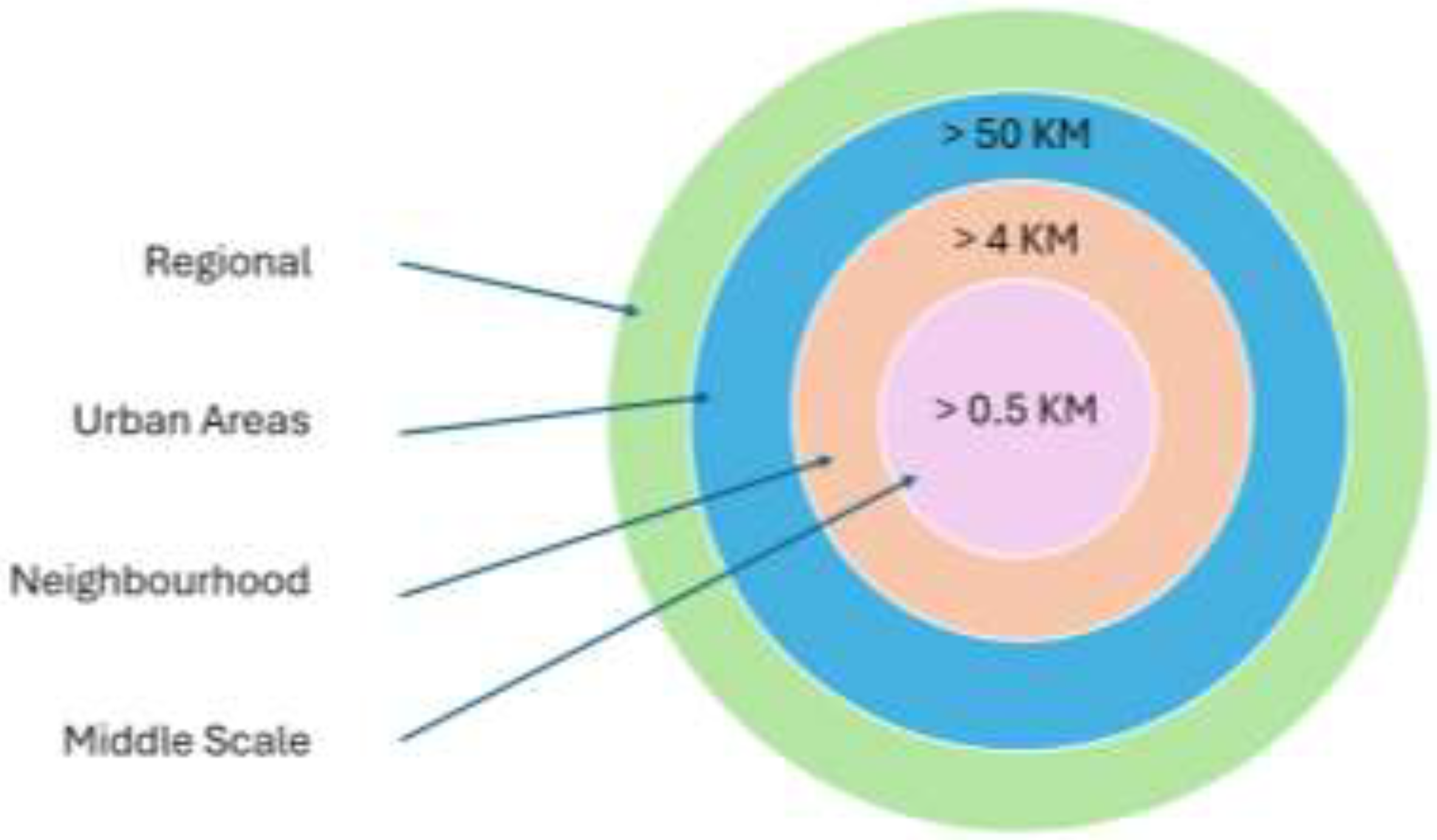
Figure 2.
- Air Quality Data Flow.
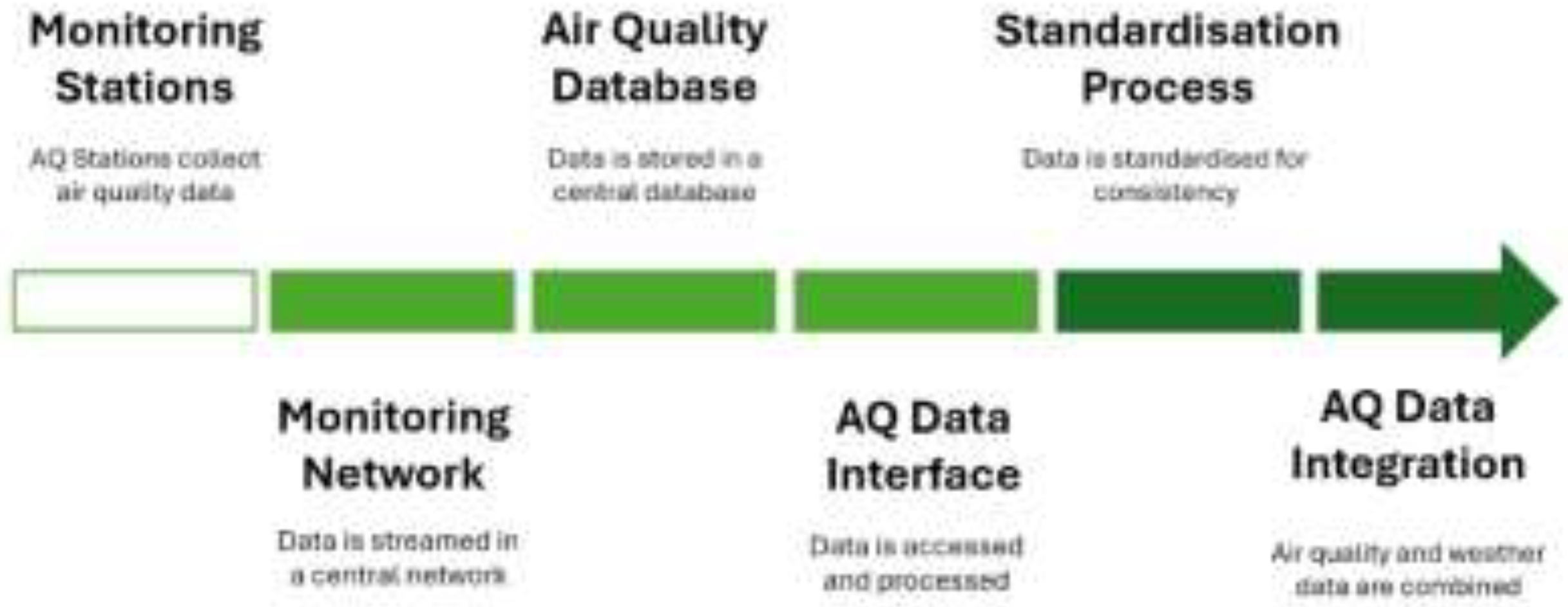
Figure 3.
- EEA vs EPA report structure.
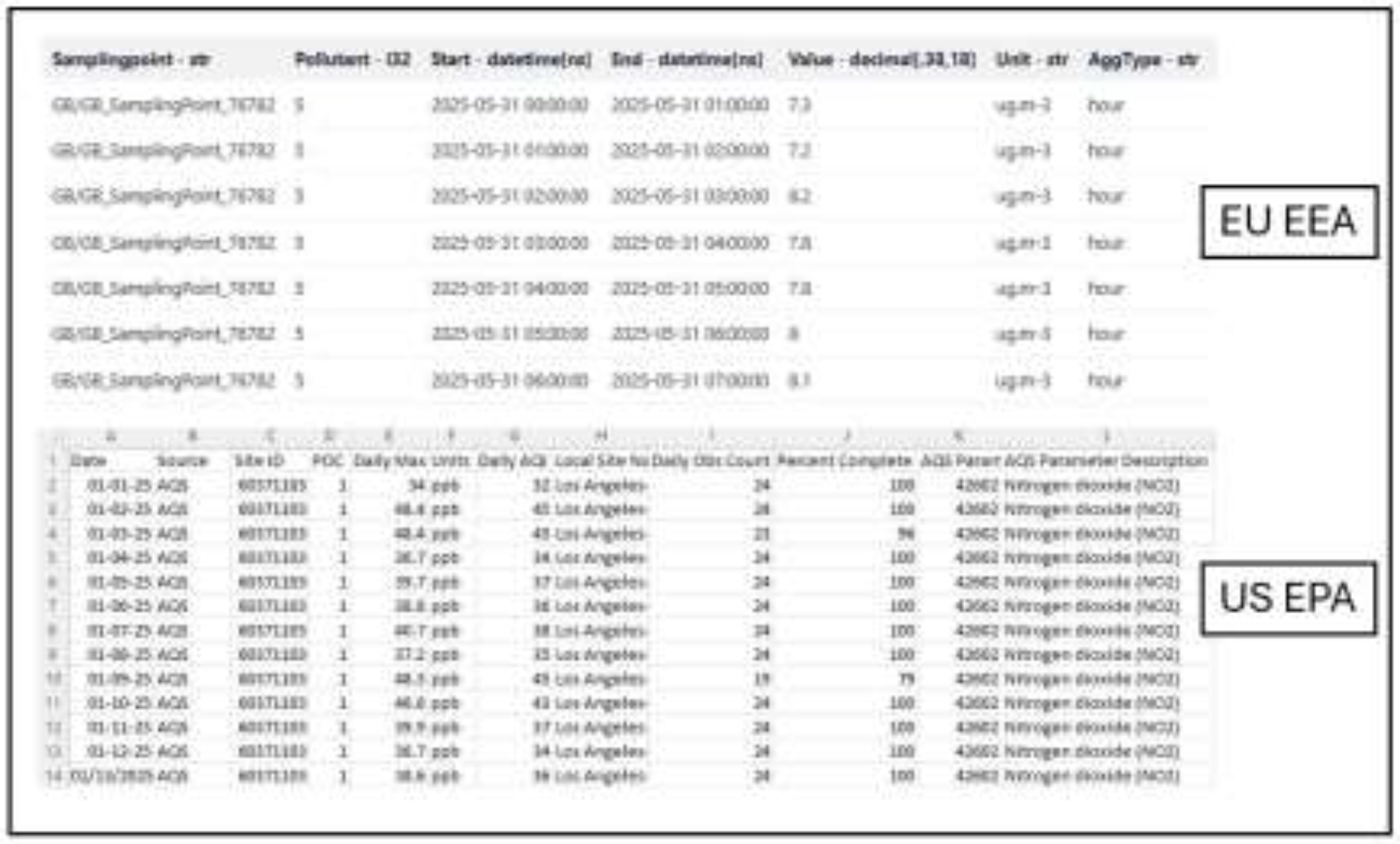
Figure 4.
- Air Quality Measuring Systems.
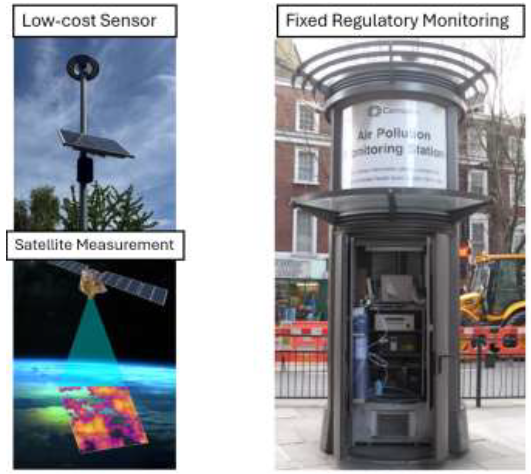
Figure 5.
- Example of star schema design.
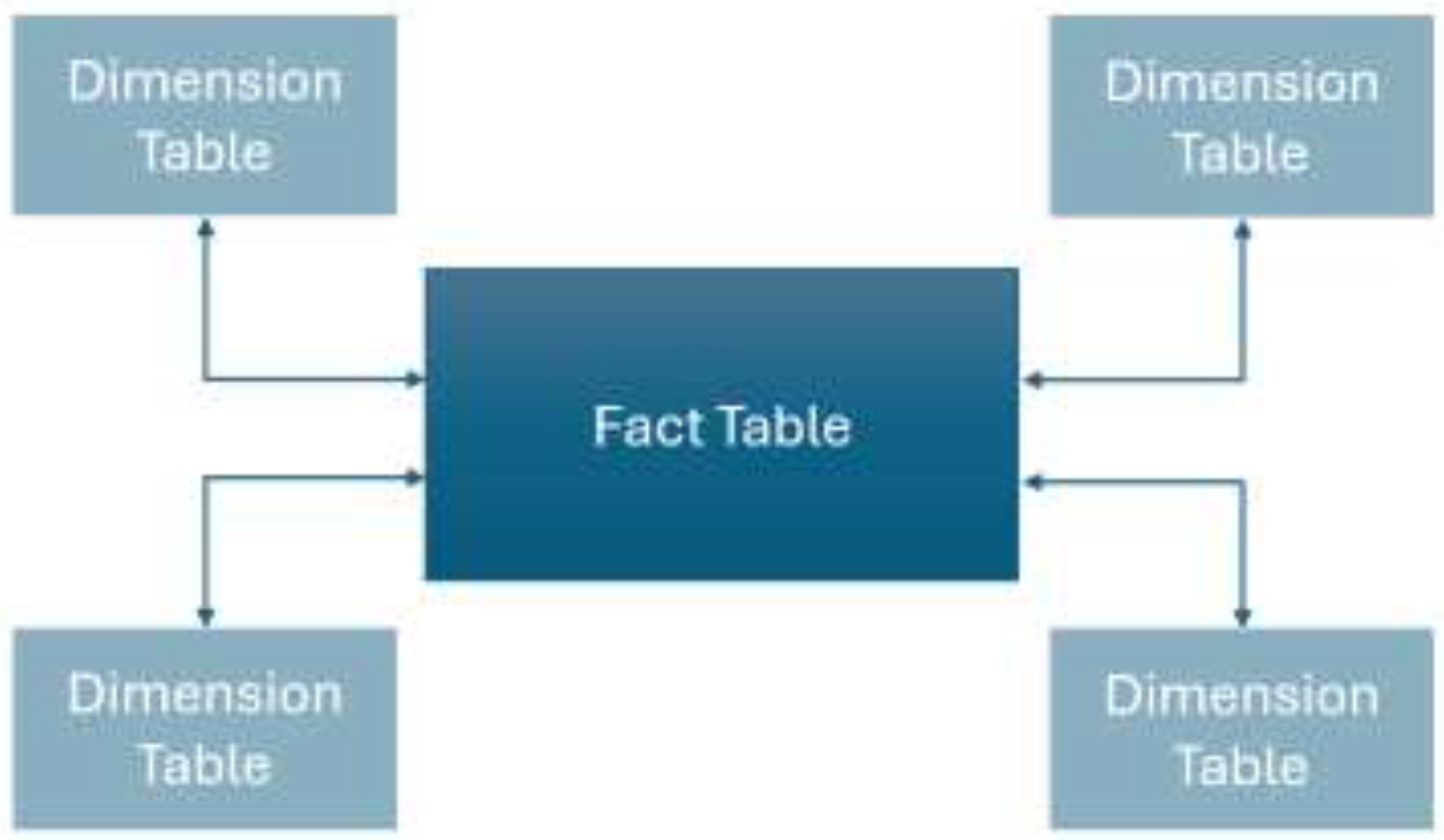
Figure 6.
- Data flow in DMT.
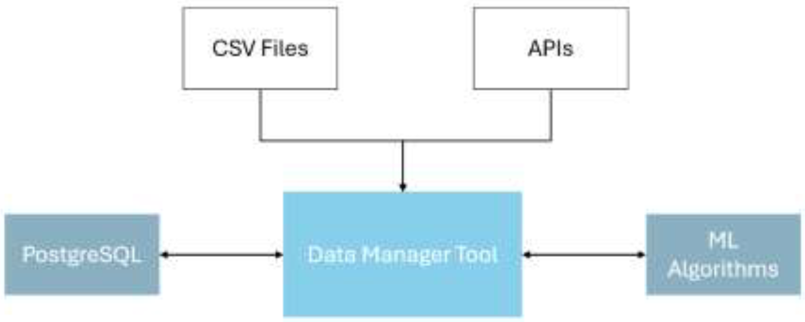
Figure 7.
– Example of an API call and JSON response.
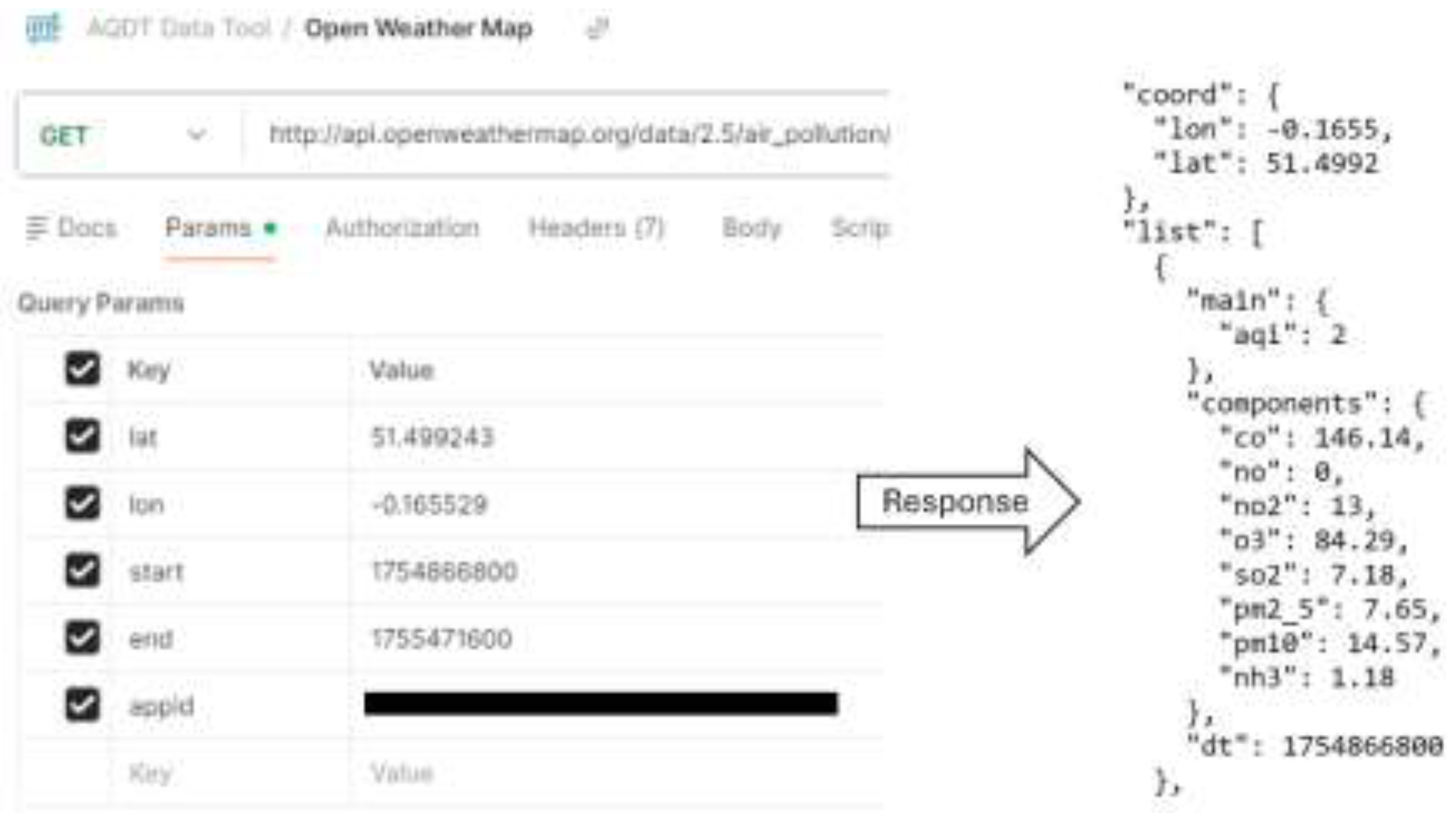

Table 1.
- Notable Air Quality Datasets.
 |
Disclaimer/Publisher’s Note: The statements, opinions and data contained in all publications are solely those of the individual author(s) and contributor(s) and not of MDPI and/or the editor(s). MDPI and/or the editor(s) disclaim responsibility for any injury to people or property resulting from any ideas, methods, instructions or products referred to in the content. |
© 2026 by the authors. Licensee MDPI, Basel, Switzerland. This article is an open access article distributed under the terms and conditions of the Creative Commons Attribution (CC BY) license (http://creativecommons.org/licenses/by/4.0/).
Copyright: This open access article is published under a Creative Commons CC BY 4.0 license, which permit the free download, distribution, and reuse, provided that the author and preprint are cited in any reuse.


