
Submitted:
22 May 2026
Posted:
25 May 2026
You are already at the latest version
Abstract
We propose a unified theoretical framework for observed redshift phenomena in astrophysics, in which gravitational and cosmological contributions arise from distinct but coexisting physical mechanisms. In this model, the gravitational field itself carries an effective mass, leading to a nontrivial field–mass structure that naturally identifies halo mass with the gravitational field mass outside baryonic sources. Independently, a cosmological redshift mechanism is derived from a relativistic quantum treatment of coherent photon propagation through an effective medium, resulting in a nonlinear closed-form energy-loss law characterized by a single effective parameter with units of Hubble’s constant. Through the definition of redshift, these two mechanisms combine multiplicatively, yielding a mathematically consistent total-redshift expression. The framework provides a unified mapping between distance and redshift for both galaxies and quasars without assuming a single dominant redshift cause. The model is constructed from explicit assumptions grounded in relativistic field dynamics and quantum coherence, and its internal consistency is demonstrated through analytic solutions and calibrated examples. Although parameter calibration is used for illustration, it does not constitute empirical validation; the focus is on formal structure, logical coherence, and theoretical plausibility. The proposed framework serves as a basis for future observational tests and theoretical refinement, illustrating how alternative physical interpretations of redshift can be formulated within a consistent relativistic setting.
Keywords:
general relativity
; gravitational redshift
; relativistic quantum theory
; cosmological redshift
MSC: 83C05; 83F05; 81Q05
1. Introduction
The increasing precision and observational reach of modern telescopes have produced datasets that expose persistent discrepancies with the predictions of standard cosmological models. These discrepancies, now commonly referred to as cosmological tensions, have reached a level of statistical and conceptual significance that motivates consideration of new physical frameworks [1]. Peculiar velocities in clusters of galaxies provide an illustration of this tension. In particular, the bulk-flow velocities reported in [2] indicate that the measured values are approximately four times larger than those predicted by the ΛCDM model.
An important challenge for any model addressing current cosmological tensions is its ability to account for the observed nonlinearity in the redshift–distance relation, as revealed in the Hubble diagram [3,4]. The analyses presented in these works were both rigorous and influential, ultimately contributing to the awarding of the Nobel Prize to their authors.
A key implication of these results was that, within the cosmological framework available at the time, the expansion of the Universe appeared to be accelerating. This introduces a conceptual difficulty, as such acceleration requires the presence of an additional energy component—commonly referred to as dark energy—that has not been directly observed and whose nature remains uncertain, particularly given its apparent persistence over cosmic time.
A recent study [5] presents a detailed reinterpretation of current cosmological observations. The author concludes that the best agreement between theory and data can be achieved by combining two frameworks: the Covarying Coupling Constants (CCC) model and the Tired-Light hypothesis. This approach is mathematically appealing and opens the possibility of exploring other hybrid models in which additional physical mechanisms may be incorporated.
However, a point of clarification may be warranted. On page 3393, the author states: “There is no need to invent new physics for the rapid formation of galaxies.” This assertion may be somewhat misleading, as the assumption of time-varying fundamental constants, as proposed in the CCC framework, already constitutes a departure from standard physics and can reasonably be interpreted as introducing new physics.
One illustrative proposal [6] introduced a novel conceptual approach that, despite criticisms concerning mathematical rigor and structural complexity, achieved sufficient internal coherence to attract serious attention within the astronomical community. Other works [7,8] pursued alternative strategies by formulating scalar potentials within a rigorous mathematical framework, obtaining solutions to the Einstein field equations [9] that exhibit meaningful correspondence with physical observables.
Collectively, these results justify the systematic exploration of additional theoretical approaches.
A redshift–distance diagram constructed from galaxy and quasar observations reveals significant deviations from the predictions of the standard ΛCDM cosmological model. The quasar CFHQS J1641+3755 [10], with a measured redshift of z = 6.047, is associated with a reported distance modulus of 43.64, corresponding to a comoving distance of approximately 5,346 Mpc. This places the object roughly ~ 5 x 10⁴ Mpc closer than the distance predicted by ΛCDM at the same redshift. Although uncertainties in quasar parameter estimation may contribute to such deviations, analogous discrepancies are also present in galaxy datasets. For example, the galaxy SDSS-II SN 13151 [11] exhibits a redshift of z = 0.388 while being reported at a distance modulus of 48.52, corresponding to approximately 50,583 Mpc—exceeding the ΛCDM prediction by an amount equivalent to a redshift shift of approximately Δz ≈ 5.1. These inconsistencies indicate the presence of either unaccounted systematic effects or fundamental limitations in the current cosmological framework, thereby motivating further theoretical and observational investigation.
A cosmological model [12] motivated by the above-mentioned discrepancies was developed with the objective of minimizing parameter correlations in the description of the observed universe. This simplification was achieved by postulating that the gravitational field possesses an effective mass. As an initial feasibility test, the model adopted a constant-density approximation, constituting a deliberate oversimplification of realistic cosmic matter distributions. In addition, it was incorrectly assumed that the principal model parameters admit no closed-form analytical solutions. The present note corrects this assumption and provides a formal analytical treatment of the model parameters. Furthermore, it introduces a graphical representation designed to facilitate direct comparison between theoretical predictions and observational data.
2. Einstein Field Equations in the Massive-Gravity Cosmological Model
We solve the Einstein field equations subject only to the physical constraints intrinsic to the problem under consideration [13]. The equations employed in this work are consistent with those derived from the Einstein–Hilbert action for a static, spherically symmetric spacetime filled with a perfect fluid. In particular, the pressure gradient follows from covariant conservation of the energy–momentum tensor, ensuring full compatibility with the standard Tolman–Oppenheimer–Volkoff framework [14]. The gravitational field is governed by the following equation:
- Spherical symmetry,
- Static spacetime, and
- An isotropic perfect fluid with vanishing shear stresses.
Under these assumptions, and adopting the Cartesian signature (+1, +1, +1, -1), the spacetime metric for the squared differential interval ds2 for a spherically symmetric source takes the form:
here, the function A(r) represents the spatial metric factor, while B(r) denotes the temporal metric factor. The components of the Ricci tensor corresponding to this metric are given by:
No assumptions are introduced beyond those strictly required by the formulation. Empirical evidence supports the existence of a well-defined limiting speed, asymptotically approached by the highest observed velocities, exemplified by the speed of light c. Within this framework, C is treated as a relativistic invariant, while the locally measured value of c is allowed, in principle, to vary with gravitational field strength. This distinction provides a mathematical advantage in the formulation of the model and admits the physical possibility of photon–photon interaction mediated through coherence states of the field.
The explicit field equations for a gravitational configuration with mass density and pressure, derived from general relativity [13] (p. 191) under the assumptions stated above, are given by:
where k is a constant to be determined later.
By dividing Equation (5a) with 2 A(r), Equation (5c) with 2 B(r), and Equation (5b) with r2, and subsequently summing the resulting expressions, one obtains—after straightforward algebraic manipulation—
Equation (6) cannot be solved at this stage because it contains two unknown functions, suggesting that both quantities are physically connected. From this point forward, numerical calculations will be employed to avoid additional assumptions that could introduce further tension between the model and observations. If the initial value A(R) at the surface of the source is determined by the average density over a region with , then the parameters defining the constant k become constrained according to k = 8 π G (3 C4)-1 by
where mb(R) and mg(R) denote the baryonic and gravitational masses enclosed within the radius R, respectively. Equation (7a) constrains the spatial factor to take the form
Numerical calculations can help visualize the physics behind this study, provided that the solutions remain continuous, have well-defined derivatives, and follow the expected behavior of each quantity, with some increasing and others decreasing with radius. For example, the gravitational mass should always increase according to
were m(1) = Mb(R) + mg(R). Equation (8) also defines the numerical cutoff of the calculation, provided that sufficient computational power and time are available, once the field density decreases below the gravitational density of open space.
The assumption that the energy-momentum tensor is conserved on this model implies
Equation (7a) is nearly identical to the corresponding function in the Schwarzschild metric. Both expressions become identical when the mass associated with the gravitational field vanishes. The connection between the present model and the Schwarzschild metric becomes even stronger if the right-hand sides of Equations (5a) and (5b) vanish. Mathematically, this could occur naturally if P(r) = ρ(r) C2, thereby removing the need to specify the individual values of these quantities. Under this condition, Equation (9) simplifies to:
The derivative of the energy density can be isolated by substituting Equation (7b), its derivative, and Equation (10) into Equation (5b). The result is
Equation (11) can be written in numerical form as
where ρ(1) represents an initial value to be adjusted according to the available experimental data.
The temporal function can be calculated numerically by substituting the energy-density values obtained from Equation (12) into the numerical form of Equation (10). The resulting expression is given by:
At this stage, it becomes necessary to define how the temporal function at the surface of the gravitational source, B(1), is calculated. The physical constraints are that this function must exist, must contain the Schwarzschild metric as the limiting case for intermediate fields, and must remain real, with a minimum value approaching zero in the maximum-density scenario. The function B(1) = 1 – 2 G m(1) (C2 R)-1 satisfies all these constraints.
Applying the Lagrange equations to the metric of the model yields three principal results: the orbital circular velocity at the source, the gravitational redshift of photons observed at infinity, and the escape velocity of a particle to the same endpoint. The corresponding expressions are
3. Results
3.1. Testing the Model
The gravitational field of the Sun was historically used as the first validation of general relativity. Although relatively weak, it was sufficient to reveal two famous deviations from Newtonian gravitational theory. The possibility that a similar situation may occur again is, at the very least, worth investigating. The solar gravitational parameter is a suitable candidate for such a test because its value is derived from many measurements.
The universal constants c and G [15], together with the equatorial radius of the Sun [16], were combined with the assumed solar mass of 1.98839 x 1030 kg and a superficial gravitational density of 1.18 x 10⁻⁹ kg m-3 to calculate the solar gravitational parameter at different locations: first, at the solar surface; second, after 63,573 increments of 9 x 10⁵ m, corresponding to the semi-major radius (SMR) of Mercury; third, after an additional 107,515 increments of 1 x 10⁶ m to reach the SMR of Venus; fourth, after 148,904 increments of the same size to the SMR of Earth; and finally, after 777,718 increments to the SMR of Jupiter. These results are presented in Table 1 together with the gravitational factors measured from the four planets considered [17].
The values presented in Table 1 are strongly correlated with the physical framework introduced in this study and suggest a gravitational scenario that is not predicted by either the Newtonian or Schwarzschild models. Even readers without specialized training can identify the pattern shown in Column 2: the solar gravitational parameter increases with distance, as expected from the present model, rather than oscillating around a single average value, as commonly assumed.
The values corresponding to Mercury, Venus, and Earth remain relatively close because these planets lie within one astronomical unit (AU) from the Sun. In contrast, Jupiter, located at more than five AU, exhibits a visible deviation from the previous three values beginning at the third decimal place. Notably, this difference lies well outside the reported uncertainty of the measured value.
If the validity and usefulness of the present model are supported by future astronomical analyses, the precision of the solar gravitational parameter could potentially be improved by avoiding the direct averaging of values derived from planetary and satellite data.
3.2. Gravitational Redshift
We now consider the characterization of a super-quasar exhibiting a large redshift despite its proximity. The spectroscopic redshift of the quasar CFHQS J1641+3755 [6] has a spectroscopic redshift of z = 6.047. has been reported as z = 6.047 [10] and z = 6.025 [18]. Some of its calculated physical parameters [19,20,21] include a central black hole of mass 2.4 x 10⁸ M⊙, a stellar and gas mass of 1011 M⊙, and the so-called M200c, defined as the mass enclosed within the radius R200c = 2 x 10²¹ m, where the mean density equals 200 times the critical density at that redshift, yielding 2.4 x 10¹² M⊙.
According to general relativity, stable circular orbits around a black hole cease to exist interior to the innermost stable circular orbit (ISCO). For a non-spinning (Schwarzschild) black hole, the ISCO radius 6 G M C-2 is approximately equal to 2.1 x 10¹² m, corresponding to an orbital velocity near 0.41 C at the inner edge of the accretion disk. Further out, in the radiatively efficient portion of the disk (e.g., at R ~ 100 rg), the Keplerian velocity decreases to approximately 0.1 C. These scaling follow directly from relativistic orbital dynamics [22,23].
The model is tested by comparing its predicted values with those expected from well-established theories. Perfect agreement is not required, since the results originate from different theoretical frameworks; however, a consistent correlation is necessary to support the validity of the proposed approach.
Special care must be taken because the present framework relies on numerical calculations, which may diverge after a sufficiently large number of iterations. A useful consistency check can be performed by graphing the parameters involved in the model. As the radius increases, the temporal factor must increase toward a maximum value of one, while the enclosed mass must increase until the density approaches that of the intergalactic medium. In contrast, the density must decrease toward the previously defined cutoff, the spatial factor must decrease toward a minimum value of one, and the redshift, orbital velocity, and escape velocity must all decrease toward zero.
These limiting values represent the asymptotic behavior expected in calculations extending over sufficiently large distances, although such long numerical integrations are often impractical. In most cases, it is preferable to begin the calculations with initial conditions chosen as close as possible to the physical region of interest to improve numerical precision and reduce computational time.
Initial values consisting of a total enclosed mass, including both baryonic and gravitational contributions, of 6.74658 x 1036 kg, confined within a radius of 1 x 10¹⁰ m, together with a density of 1 x 10⁴ kg/m3 at that radius, were used to model the properties of the quasar CFHQS J1641+3755. Using 600,000 numerical steps with radial increments of 3 x 10⁶ m, it was possible to obtain the data presented in Table 2.
3.2. Cosmological Redshift
Cosmological data from galaxies exhibiting small redshifts, even at large distances, can help constrain the modeling of the cosmological redshift. For example, consider the galaxy SDSS-II SN 13151 [11], started in the Introduction. Although this problem has been addressed in detail previously [24], we provide here a streamlined derivation and clarify the adaptation of the main parameters to the formalism used in the present work. While the standard relativistic calculations of Dirac were applied successfully to particles with spin-½, and that could create the impression that those derivations cannot be directly applicable to photons, the equation used in this work arises as a particular solution of a relativistic quantum framework under the physically motivated condition of our problem and that solution justify the understanding of the general applicability of the Dirac derivations. Therefore, any criticism based solely on the formal Dirac structure should be reconsidered in light of the specific assumptions and derivation underlying this solution.
Under the following assumptions:
- The coherence of the light state depends on the interaction of each photon with surrounding photons in all directions.
- A universal speed limit C exists. According to special relativity, the speed of light c corresponds to this limit; however, in the present framework, c does not necessarily coincide exactly with C. Instead, c < C, while remaining extremely close to C, so that no contradiction arises with current experimental knowledge. From this perspective, c may be treated as a local variable.
- The original relativistic invariant derivation introduced by Dirac, rather than the specific equation now known as Dirac’s equation [25], may be extended to a more general expression. Its formalism may then be applied to any potential, including electric potential acting on charges e and gravitational potential acting on rest masses m.
Following from assumption 3:
here, i2 = -1, ћ is the reduced Planck constant (h/2π), ψ is the state function and t denotes time. The vector α is a 4 x 4 matrix containing the Pauli matrices, p is the four-momentum vector, β is another 4 x 4 matrix populated with positive and negative ones and zeros, and ϕ and A are the gravitational scalar and vector potentials, respectively. In the present treatment, is assumed for photons because of their electrically neutral nature.
Applying cylindrical coordinates to a beam of light, Equation (17) yields the following four coupled equations,
Here
here, the + and - symbols correspond to photons in particle-like and antiparticle-like states, respectively
The four components of Equation (18) cannot be reduced through a non-relativistic approximation in the manner originally applied by Dirac to electrons. These four independents, or overlapping, states indicate that photons possess spin-1 and two orthogonal polarization states, in agreement with the standard quantum-mechanical description of photons. One polarization state is transverse and extends along the radial direction, perpendicular to the direction of propagation, while the other is aligned with the propagation direction z and is commonly referred to as longitudinal.
In [24] was shown that a beam of photons propagating in a coherent state must lose energy. The corresponding effect, expressed as a redshift in the notation adopted throughout this paper, is
here, d denotes the distance traveled by the photon beam. Equation (19) exhibits several notable conditions that, in principle, support the validity of its derivation. First, Planck’s constant ћ cannot be zero; otherwise, any photon would lose all its energy immediately upon interaction with another photon. This is consistent with the quantum condition that photons cannot exist in the limit ћ ⟶ 0. Second, if c = C, implying that the photon mass is zero, photons would retain their energy regardless of travel distance, as it is assumed now.
It is intriguing to note that m C2 ћ -1 approximates 2 H0 when Equation (19) is expanded for small distances d, consistent with Hubble’s law. This equivalence would hold if all galactic and quasar redshifts were purely cosmological; however, such a scenario is not assumed in the present analysis.
It is convenient to combine the three constants in Equation (19) into a single effective constant, as shown below,
here, Χ ≡ m C2 ћ -1 represents the photon energy leakage rate and has the same units as Hubble’s constant.
3.3. Total Redshift
The redshift is defined as the fractional difference between the emitted energy and the detected energy, minus one. Performing the algebra and neglecting other physical effects, such as the Doppler effect, yields the following relationship:
The value of Χ was determined by adjusting the model to ensure that all quasar and galaxy redshifts shown in Figure 1 were reproduced by Equation (21). The figure reveals a semi-symmetric distribution of quasars and galaxies, including objects with relatively low redshifts that follow a similar semi-linear trend as those with higher redshifts.
The two independent parameters in Equation (21), Χ and the maximum gravitational redshift, are defined by the extrema of the quasar and galaxy distribution. Specifically, Χ = 2 km s-1 Mpc-1, and the maximum gravitational redshift is zgrav_max = 5.8. The lower bound is anchored by the galaxy SDSS-II SN 13151, while the upper bound is determined by the quasars CFHQS J1641+3755, ULAS J1120+0641, J1342+0928, and the galaxy GRB 090429B, as illustrated in Figure 1.
For the quasar CFHQS J1641+3755, Equation (20) predicts a cosmological redshift of zcosm = 0.035. Combined with the gravitational redshifts of zgrav = 5.7874 and zgrav = 5.087, the total redshifts according to Equation (21) are ztot = 6.025 and ztot = 6.047, in agreement with the observed values [10,18].
It should be emphasized that this agreement does not constitute a validation of the model. The agreement between the modeled and observed redshifts was obtained by manually adjusting the initial radius, the mass enclosed within that radius, and the gravitational-field density at the same radius, demonstrating that the model can, in principle, account for the observed redshift.
4. Discussion
The number of galaxies and quasars in the universe, the range of their distances from the observer, and the spread of redshift detected in their emitted radiation are sufficiently large that the underlying explanation must be as simple as possible. Nevertheless, it is unsurprising that a single cause may not account for all observed phenomena. A natural next step is to consider a combination of two causes; however, this approach introduces the challenge of determining whether their contributions are additive, multiplicative, or otherwise coupled. Alternatively, one may posit a single physical mechanism that manifests differently across distinct locations or times—for instance, one effect could be local, while the other is non-local.
In the present work, our central hypothesis is that any field possesses mass. According to the principles of relativity, this implies that any speed associated with such fields must be, at least microscopically, less than the universal speed limit. The consequences of this assumption vary according to the dynamics of each field, as detailed below.
Locally, if the gravitational field possesses mass, its density and pressure will be dominated by the baryonic matter in solid or liquid form, as recently discussed [8]. In this paper, a new solution to the general relativity equations outside a baryonic source was introduced. Specifically, it was found that the function describing the gravitational field at different locations allows the identification of the so-called dark matter mass with the gravitational field mass.
It is assumed that the properties of the gravitational field density are not overridden by the baryonic dust and gas within it, but rather coexist under a ratio of approximately ten, consistent with the baryon fraction suppression relative to the cosmic mean [29]. It should be noted that the gravitational field is expected to follow the superposition principle; therefore, the gravitational field mass associated with all local sources, such as stars, can be added linearly.
To illustrate the significance of this halo mass, we consider a quasar example. radiation emitted from the quasar’s disk would emerge with a redshift of only 0.066. According to the standard cosmological model, a redshift of approximately z ~ 1 would be expected for that quasar; however, observations [19,20,21] report a redshift greater than z =6.025.
The energetic state of a coherent light beam can be described by solving the relativistic quantum equation for a cylindrical ensemble of energetically coupled particles. Nevertheless, gravitational and cosmological redshifts are physically independent phenomena; their contributions cannot be added linearly due to the standard definition of redshift. Instead, the definition inherently combines these effects multiplicatively, as is typical for correlated processes.
This multiplicative relationship simplifies the modeling, as the astronomical data in Figure 1 exhibits a similar distribution of points at both low and high redshifts. This pattern is consistent with the independent nature of the two mechanisms: although Figure 1 may suggest that the gravitational redshift simply adds to the cosmological redshift, but the energy of the beam is, in fact, first influenced by the local gravitational field of the source and subsequently modified by the coherence state of the beam during propagation.
The static model of the universe presented here is mathematically self-consistent, does not contradict any currently known physical laws, and appears robust with respect to variations in its parameters. To illustrate this assertion, one may consider, for example, the mass of the photon. Equation (22) by expressing this relationship:
implies that the photon mass is constant. Using the constraint that the universal speed limit C exceeds but is extremely close to the speed of light c, yields a photon mass of approximately around 2 x10-70 kg. This value is smaller than the currently established upper limit for the photon mass (PMUL = 3 x10-63 kg) [30].
Beyond this, the model may primarily serve as a convenient numerical tool for astronomers, rather than providing direct predictive power. This is plausible due to the additive nature of the two contributing factors discussed here. Specifically, if the redshift is dominated by the ΛCDM description, then the gravitational and cosmological contributions considered in the present work—both positive—cannot reduce the ΛCDM values. Consequently, this the ΛCDM model is structurally incapable of accounting for the region below the green curve in Figure 1.
If this work proves of interest to readers, it may inspire further investigation of three questions that remain unresolved due to limitations of time and resources:
- Verifying whether the gravitational solution proposed in the present model satisfies additional consequences of general relativity, such as the existence of a mathematical relationship between the baryonic mass of a body and the quantity of gravitational mass contained within it. Such a relationship could help determine the density of the gravitational field at the surface of the body.
- Examining whether data from modern telescopes remain consistent with the red and blue dashed curves in Figure 1.
- Investigating why most galaxies and quasars exhibit a higher concentration near the green curve representing the ΛCDM model in Figure 1.
5. Conclusions
This work presents a theoretical framework in which gravitational, and coherence-based mechanisms contribute jointly to observed redshift phenomena. The model is constructed from a small set of physical assumptions: the existence of mass associated with physical fields, relativistic constraints on universal speed limits, and the applicability of relativistic quantum formalisms to coherent photon propagation. These assumptions lead to modified gravitational field dynamics, a nontrivial field-mass structure, and the emergence of multiple redshift channels.
A new solution to the Einstein field equations outside baryonic sources was introduced, allowing the identification of gravitational field mass with effective halo mass. Independently, a cosmological redshift mechanism was derived from a relativistic quantum treatment of coherent photon beams, yielding a nonlinear energy-loss formulation characterized by a single effective parameter. Through the definition of redshift, these mechanisms combine multiplicatively, producing a total redshift expression that is structurally consistent and mathematically well-defined.
The agreement between the model and selected observational data is achieved through parameter calibration and therefore does not constitute empirical validation. The present results should be interpreted as proof of theoretical consistency and internal coherence rather than as observational confirmation. No claim is made that the framework supersedes the CDM model, which remains the standard cosmological description.
The primary contribution of this work lies in establishing a unified formal structure in which multiple redshift mechanisms can coexist without internal contradiction, and in demonstrating that such a structure can be constructed within relativistic and quantum-consistent principles. Future work must focus on observational discrimination, independent parameter determination, and predictive testing against high-precision cosmological datasets to assess the physical viability of the model.
In summary, the novelty of this work lies in extending two established ideas: additional gravitational potentials associated with massive sources, and effective gravitational interactions among photons in a propagating beam that remains in a near state of relative rest. These effects lead to a reduction in photon energy that can be consistently described within general relativity and quantum mechanics.
Strong gravitational fields may thus produce effects analogous to those attributed to dark matter, while the associated redshift function quantifies their impact on photon energy. Over cosmological distances, the cumulative effect reproduces the observed distance–redshift relation for galaxies and quasars. This result is founded on rigorous calculations.
If supported observationally, the model must still address key challenges, including baryon acoustic oscillations and the apparent stability of cosmological scales. Any temporal variation of the cosmic microwave background temperature would provide insight into large-scale dynamics.
More broadly, the scope of this framework is to motivate further exploration of the interplay between general relativity and relativistic quantum mechanics, with possible implications for a unified theoretical description.
References
- Valentino, E.; et al. The CosmoVerse White Paper: Addressing observational tensions in cosmology with systematics and fundamental physics. Phys. Dark Universe 2025, 49, 1–263. [Google Scholar] [CrossRef]
- Watkins, R.; et al. Analysing the large-scale bulk flow using cosmicflows4: increasing tension with the standard cosmological model. MNRAS 2023, 524, 1885–1892. [Google Scholar] [CrossRef]
- Riess, A. G.; et al. OBSERVATIONAL EVIDENCE FROM SUPERNOVAE FOR AN ACCELERATING UNIVERSE AND A COSMOLOGICAL CONSTANT. Astron. J. 1998, 116, 1009–1038. [Google Scholar] [CrossRef]
- Perlmutter, S.; et al. MEASUREMENTS OF Ω AND Λ FROM 42 HIGH-REDSHIFT SUPERNOVAE. Astrophys. J. 1999, 517, 565–586. [Google Scholar] [CrossRef]
- Gupta, R. A. JWST early Universe observations and VCDM cosmology. MNRAS 2023, 524, 3385–3395. [Google Scholar] [CrossRef]
- Jusufi, K.; Singleton, D. Regular black holes with gravitational self-energy as dark matter. ArXiv. 2025. Available online: https://arxiv.org/pdf/2509.13335.
- Cembranos, J.A.R.; Luis Díaz-Giménez, L. Hydrodynamical Misner–Sharp Formulation for Gravitational Collapse in Scalar–Tensor Theories ArXiv. 2025. Available online: https://arxiv.org/pdf/2512.17526.
- Das, S.; Radinschi, I.; Chattopadhyay, S. Modified Gravity Description of Neutron Star in the f(R) Framework. Axioms 2023, 12, 234. [Google Scholar] [CrossRef]
- Einstein, A. The field equations of gravitation, 1er ed., Publisher: Princeton University Press, Einstein.papers.press.princeton.edu (Prusian Academy of Science 1914-1917), USA. Available online: https://einsteinpapers.press.princeton.edu/vol6-trans/129.
- Ochsenbein, F. The VizieR database of astronomical catalogues, Publisher Centre de Donnees astronomique de Strasbourg (CDS) 2020.
- NASA/IPAC Extragalactic Database. NED30.5.1-D-17.1.2-20200415 V2. NASA. 2020. Available online: https://ned.ipac.caltech.edu/Archive/Distances/ (accessed on 22 May 2025).
- Parra, J. L. Quasars as strong standard candle candidates. Int. J. Mod. Phys. A 2025, 40, 1–8. [Google Scholar] [CrossRef]
- Walecka, J.D. Introduction to General Relativity, 1st ed., World Scientific Publishing Co. Pte. Ltd. 2007, pp. 190-191.
- Oppenheimer, J. R.; Volkoff, G.M. On Massive Neutron Cores. Phys. Rev. 1939, 55, 374–382. [Google Scholar] [CrossRef]
- List of physical constants - Wikipedia.
- Sun - Wikipedia.
- Park; et al. The JPL Planetary and Lunar Ephemerides DE440 and DE441. Astron. J. 2021, 161, 105–129. [Google Scholar] [CrossRef]
- Vito, F.; et al. , Intervening nuclear obscuration changing the X-ray look of the z ≈6quasi-stellar object CFHQS J164121+375520. Astron. Astrophys. 2025, 694, L16, 1–5. [Google Scholar] [CrossRef]
- Willott, C.J.; et al. EDDINGTON-LIMITED ACCRETION AND THE BLACK HOLE MASS FUNCTION AT REDSHIFT 6. Astron. J. 2010, 140, 546–560. [Google Scholar] [CrossRef]
- Fan, X.; et al. A SURVEY OF z > 5.8 QUASARS IN THE SLOAN DIGITAL SKY SURVEY. I. DISCOVERY OF THREE NEW QUASARS AND THE SPATIAL DENSITY OF LUMINOUS QUASARS AT z ~ 6. Astron. J. 2001, 122, 2833–2849. [Google Scholar] [CrossRef]
- Venemans, B.P.; et al. DISCOVERY OF THREE z > 6.5 QUASARSI NTHE VISTA KILO-DEGREE INFRARED GALAXY (VIKING) SURVEY. Astron. J. 2013, 779, 24–37. [Google Scholar] [CrossRef]
- Shakura, N.I.; Sunyaev, R.A. Black Holes in Binary Systems: Observational Appearances; Cambridge University Press, 1973; pp. 155–164. [Google Scholar] [CrossRef]
- Abramowicz, M.A.; Fragile, P.C. Foundations of Black Hole Accretion Disk Theory. Living Rev. Relativ. 2013, 16, 1–88. [Google Scholar] [CrossRef] [PubMed]
- Parra, J.L. Photonic Gravitational Interactions from a Quantum Point of View. Opt. Photonics J. 2021, 11, 12–21. [Google Scholar] [CrossRef]
- Dirac, P. The Quantum Theory of the Electron. Proc. R. Soc. A. Proc. R. Soc. Lond. 1928. A 117, 610–624. [CrossRef]
- Lusso, E. Tension with the flat λCDM model from a high-redshift Hubble diagram of supernovae, quasars, and gamma-ray bursts. Astron. Astrophys. 2019, 4, 1–5. [Google Scholar] [CrossRef]
- E. Lusso, E. Quasars as standard candles III. Validation of a new sample for cosmological studies. Astron. Astrop. 2020, 642, 1–24. [Google Scholar] [CrossRef]
- Risality, G. Cosmological constraints from the Hubble diagram of quasars at high redshifts. Nat. Astron. 2019, 3, 272–277. [Google Scholar] [CrossRef]
- Aghanim, N.; Akrami, Y.; Ashdown, M.; Aumont, J.; Baccigalupi, C.; et al. Planck 2018 results. VI. Cosmological parameters. Astron. Astrophys. 2020, 641, A6. [Google Scholar] [CrossRef]
- Chibisov, G.V. Astrophysical Upper Limits on the Photon Rest Mass. Sov. Phys. Uspekhi 1976, 19, 624–626. [Google Scholar] [CrossRef]
Figure 1.
Redshift–distance relation for 2,417 quasars [10,26,27,28] (blue circles) and 6,880 galaxies [11] (red circles), together with two models. The green curve was generated with the assistance of OpenAI’s ChatGPT-13, calibrated to the ΛCDM model with parameters H0 = 73 Km s-1 Mpc-1, Ωm = 0.3, and ΩΛ = 0.7. The dashed red and blue curves correspond to Equation (21) with a gravitational redshift of 0 and 5.8, respectively. The model reproduces all displayed points when Χ = 2 Km s-1 Mpc-1.
Figure 1.
Redshift–distance relation for 2,417 quasars [10,26,27,28] (blue circles) and 6,880 galaxies [11] (red circles), together with two models. The green curve was generated with the assistance of OpenAI’s ChatGPT-13, calibrated to the ΛCDM model with parameters H0 = 73 Km s-1 Mpc-1, Ωm = 0.3, and ΩΛ = 0.7. The dashed red and blue curves correspond to Equation (21) with a gravitational redshift of 0 and 5.8, respectively. The model reproduces all displayed points when Χ = 2 Km s-1 Mpc-1.
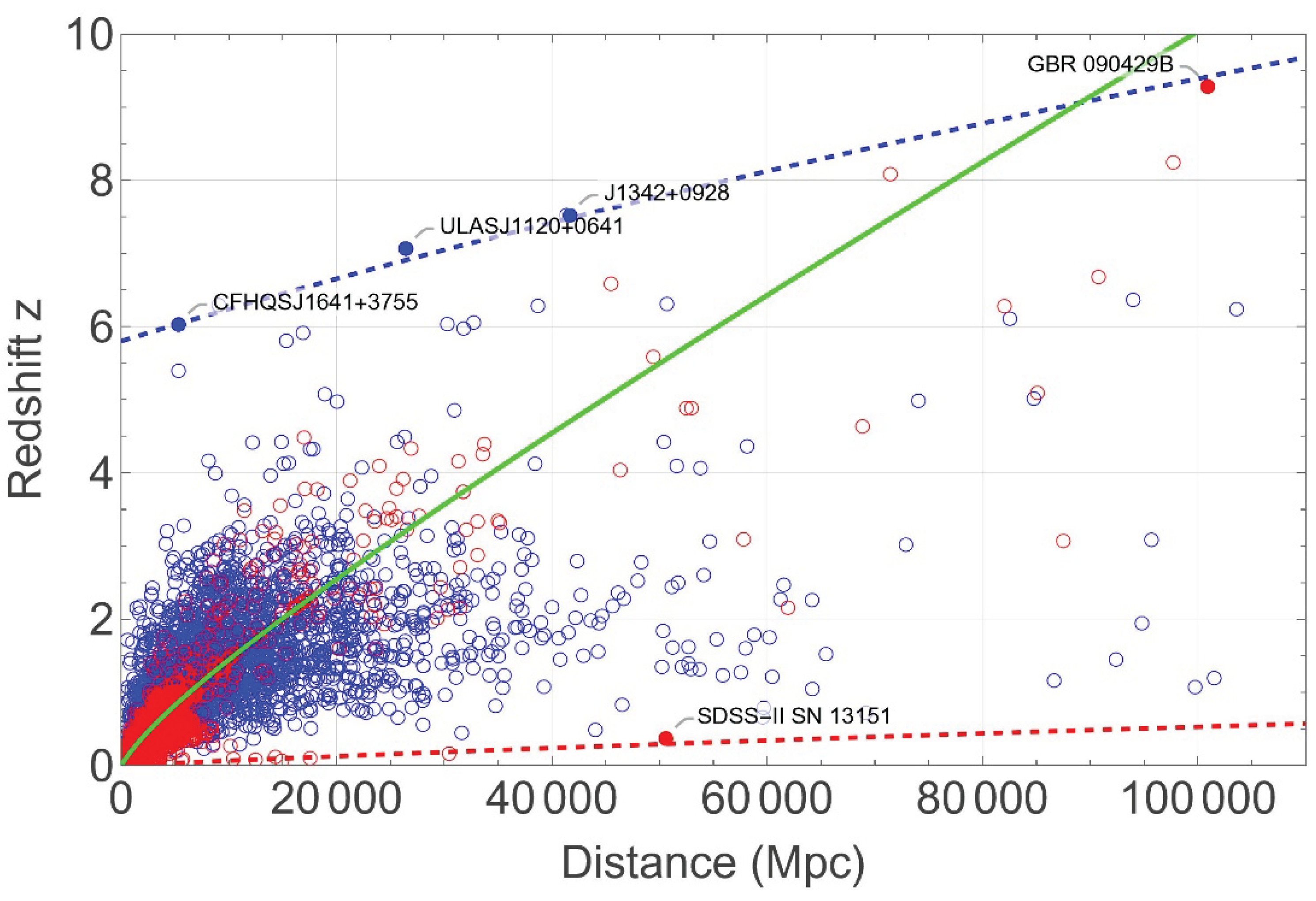

Table 1.
The values reported in the last three columns retain the number of significant figures necessary to illustrate the variation of the gravitational-field density with distance in Column 2 and to highlight the differences between the G M⊙ values derived from Earth and Jupiter in Columns 3 and 4.
Table 1.
The values reported in the last three columns retain the number of significant figures necessary to illustrate the variation of the gravitational-field density with distance in Column 2 and to highlight the differences between the G M⊙ values derived from Earth and Jupiter in Columns 3 and 4.
| Body | Field Density | Observed G M⊙ | Modeled G M⊙ |
|---|---|---|---|
| Units | 10-9 kg m-3 | 1020 m3 s-2 | 1020 m3 s-2 |
| Sun | 1.18000001 | 1.3271111 | 1.327111 |
| Mercury | 1.17999511 | 1.327124 | 1.327112 |
| Venus | 1.17999499 | 1.327126 | 1.327116 |
| Earth | 1.17999496 | 1.327129 | 1.321270 |
| Jupiter | 1.17999494 | 1.328677 | 1.328683 |
1 This value is based on the quantity assumed in the present model and is included here to facilitate comparisons.
Table 2.
Modeled gravitational parameters for the quasar CFHQS J1641+3755. The primary purpose of this table is to highlight the results presented in Row 4, where, despite the large separation between the two circular regions of approximately 10 AU, the redshifts of the light beams emitted from both regions remain remarkably close in value, consistent with astronomical observations.
Table 2.
Modeled gravitational parameters for the quasar CFHQS J1641+3755. The primary purpose of this table is to highlight the results presented in Row 4, where, despite the large separation between the two circular regions of approximately 10 AU, the redshifts of the light beams emitted from both regions remain remarkably close in value, consistent with astronomical observations.
| Parameter | Inner Circle | Outer Circle |
|---|---|---|
| Radius (m) | 7.714870 x 10¹¹ | 1.441597 x 10¹² |
| Mass (kg) | 6.80318 x 1036 | 7.11238 x 1036 |
| Density (kg m-3) | 0.0292256 | 0.0290430 |
| Redshift | 5.8087000 | 5.7874000 |
| A(r) | 1.01317000 | 1.0071100 |
| B(r) | 0.0215710 | 0.0217070 |
| Orbital β | 0.0814822 | 0.0611952 |
| Escape β | 0.9891560 | 0.9890870 |
Disclaimer/Publisher’s Note: The statements, opinions and data contained in all publications are solely those of the individual author(s) and contributor(s) and not of MDPI and/or the editor(s). MDPI and/or the editor(s) disclaim responsibility for any injury to people or property resulting from any ideas, methods, instructions or products referred to in the content. |
© 2026 by the authors. Licensee MDPI, Basel, Switzerland. This article is an open access article distributed under the terms and conditions of the Creative Commons Attribution (CC BY) license (http://creativecommons.org/licenses/by/4.0/).
Copyright: This open access article is published under a Creative Commons CC BY 4.0 license, which permit the free download, distribution, and reuse, provided that the author and preprint are cited in any reuse.