Submitted:
12 February 2026
Posted:
14 February 2026
You are already at the latest version
Abstract
This study investigates the relationship between market volatility, especially VIX levels and spikes above 45, and future equity returns. The analysis stems from the tactical decisions investors face during sharp market drawdowns. We explore whether volatility indicators, combined with investor sentiment measures, can inform shifts from defensive to opportunistic portfolio positions. Using U.S. data from 2008 to 2025, we test linear regression, logistic regression, and GARCH (1,1) models to evaluate return predictability. Results show that extreme VIX spikes offer contrarian signals, with significant positive returns over three-month horizons. Logistic regression confirms significance over both three-month and one-year periods. These findings remain robust after controlling for valuation, credit spreads, PMI, sentiment ratios, and interaction effects. While GARCH captures conditional variance, it lacks forward-looking predictive power in high-stress regimes. Overall, the evidence suggests that volatility timing merits consideration as part of a tactical allocation framework. Our findings also contribute to the market efficiency debate by integrating market expectations with economic indicators for risk-aware decision-making.
Keywords:
implied volatility
; VIX spikes
; return predictability
; behavioral finance
1. Introduction
Traders often pursue contrarian strategies during significant market drawdowns, anticipating a reversion to historical valuations and seeking excess risk-adjusted returns. This behavior implies a tactical asset allocation shift from defense to offense as the market enters and exits crisis phases. Building on this, we examine whether volatility indicators, especially the VIX and extreme levels (above 45), offer predictive insight into future equity market returns. We also evaluate whether forward returns and behavioral indicators, together with volatility signals, relate to the conditional probability of entering a high-volatility regime.
Substantial academic work has explored the information content of implied volatility. The CBOE Volatility Index® (VIX®), often labeled the “investor fear gauge,” reflects market expectations of near-term volatility from S&P 500 option prices. While the VIX’s forecasting power in modeling time-varying risk premia is well-documented (e.g., Whaley, 2000; Bollerslev et al., 2009), the role of extreme VIX levels in predicting future returns remains less understood. VIX spikes beyond 45—seen only during severe dislocations—typically signal panic and behavioral overreaction, which may create contrarian opportunities as prices diverge from fundamentals.
This research tests whether instances of VIX > 45 produce statistically and economically significant forward return reversals over three- and twelve-month horizons. Such reversals may arise from behavioral overreactions that push prices below intrinsic value, creating entry points for tactical allocators. Theoretical foundations supporting this include investor sentiment, bounded rationality, and volatility feedback effects (Barberis et al., 1998; Daniel et al., 1998; Zhou, 2018).
We use three modeling approaches applied to U.S. equity data from 2008 to 2025. First, OLS regressions test whether VIX elevations predict forward returns. Second, logistic regressions estimate the conditional probability of entering high-volatility regimes based on valuation, sentiment, and return-based indicators. Third, a GARCH (1,1) model assesses whether time-varying conditional volatility adds explanatory power in forecasting equity returns.
Initial diagnostics reveal a negative and statistically significant relationship between volatility and forward returns, while sentiment variables show a positive association. The OLS model serves as a baseline to evaluate model fit and as a benchmark for the more advanced logistic and GARCH specifications (Wooldridge, 2019). The logit model captures nonlinear regime-shift probabilities, while GARCH models volatility dynamics over time. Together, these approaches test the predictive efficacy of both threshold-based and continuous volatility measures.
This study contributes to the asset pricing literature in three ways. First, it shows that extreme implied volatility levels can function as contrarian signals for future return reversals. Second, it compares discrete regime-based and continuous volatility forecasting methods. Third, it provides investors and risk managers with a transparent, interpretable signal that coincides with market stress and asset repositioning opportunities.
1.1. Theoretical Background and Hypotheses Development
The research framework integrates neoclassical asset pricing theory with behavioral finance concepts to develop a unified perspective. The volatility feedback model by French, Schwert, and Stambaugh (1987) suggests that rising expected volatility demands higher returns, triggering immediate price declines. These price drops may reverse if volatility shocks are temporary or sentiment-driven, as risk perceptions tend to normalize.
Behavioral finance theories, notably Barberis et al. (1998) and Daniel et al. (1998), show that investors outweigh recent negative information in uncertain periods, leading to overreaction and temporary mispricing. While GARCH models can detect shifts in conditional variance, they often fall short in capturing abrupt regime changes or sentiment-driven shocks. Our hypotheses emerge from this synthesis of theoretical foundations.
Building on these theoretical perspectives, we propose the following hypotheses:
- Hypothesis 1 (Contrarian Returns):
- Extreme implied volatility conditions, as indicated by a VIX level exceeding 45, are followed by significantly positive equity market returns over the subsequent three-month and one-year horizon.
This hypothesis is grounded in the notion that extreme VIX levels represent a market regime characterized by investor fear and risk aversion1. In line with behavioral models, we expect that such environments lead to exaggerated selloffs, which subsequently reverse as investor sentiment stabilizes. Thus, high VIX levels may serve as contrarian signals, markers of excessive pessimism and future return potential.
1.1.1. Motivation for Testing Hypothesis 1
When the VIX exceeds 45, it often precedes strong three-month and one-year equity returns. Such extreme levels reflect heightened fear and risk aversion, forming the basis of this study’s hypothesis. Behavioral finance suggests exaggerated selloffs in these conditions may reverse once sentiment normalizes. Thus, elevated VIX readings may act as contrarian signals of future gains.
This study tests whether VIX > 45 reliably predicts return reversals. While the VIX is widely accepted as a fear gauge, its forecasting accuracy is debated. Some studies argue that extreme volatility signals oversold conditions and offer entry points for contrarian investors (Bekaert & Hoerova, 2014; Blitz et al., 2019).
Sharp VIX spikes often coincide with market overreactions. Research by Ngoc (2014) and Pan and Poteshman (2006) shows that surges in implied volatility are frequently followed by recoveries, supporting mean reversion. Bekaert and Hoerova (2014) and Bollerslev et al. (2015) also document positive returns following panic episodes.
These findings suggest prices diverge from fundamentals during crises, then correct. For asset managers, recognizing VIX extremes as contrarian signals can enhance tactical allocation. This study evaluates whether VIX > 45 reflects true macroeconomic risk or investor overreaction.
Understanding these dynamics helps investors design volatility-based strategies to exploit dislocations. Given the VIX’s role in risk models, its predictive behavior during stress events is essential for tactical positioning.
- Hypothesis 2 (Volatility Spike Predictability):
- Prior market conditions, including negative short-term returns, elevated trailing volatility, and bearish investor sentiment, significantly increase the probability of observing a VIX spike (VIX > 45).
Consistent with regime-switching frameworks and models of sentiment contagion2, we hypothesize that extreme volatility events (defined as VIX > 45) do not arise randomly but are preceded by identifiable market conditions. Specifically, when short-term equity returns are negative, trailing volatility is elevated, and investor sentiment deteriorates, the probability of transitioning into a high-volatility regime increases substantially. This view assumes that VIX spikes emerge from internal market dynamics rather than exogenous shocks, and that these transitions can be forecasted using observable indicators. The theoretical foundation aligns with models that treat volatility as an endogenous feature of market behavior, driven by feedback loops between declining asset prices, rising uncertainty, and behavioral responses from market participants3.
1.1.2. Motivation for Testing Hypothesis 2
The identification of market signals preceding extreme volatility events—particularly when the VIX surpasses 45—is essential for asset pricing, risk management, and tactical decision-making. While the VIX is widely studied as a proxy for investor fear and market uncertainty, limited research evaluates whether observable signals such as trailing returns, realized volatility, and sentiment deterioration can forecast such spikes. This study addresses that gap.
Volatility shocks often emerge from compounding negative market signals. Prior research (Bekaert & Hoerova, 2014; Manela & Moreira, 2017) finds that fear and macro uncertainty influence both VIX levels and variance risk premia. Feedback loops driven by sentiment reinforce volatility surges. Lagged returns, volatility clustering, and sentiment metrics—like put-call ratios and volatility derivative positioning—offer partial predictability of extreme regimes (Kelly et al., 2019; Han, 2008).
Testing whether weak returns, high trailing volatility, and pessimism can jointly anticipate VIX surges enables more effective hedging and portfolio stress testing. This study also evaluates whether regression-based models outperform traditional time-series models like GARCH (1,1) in these contexts. It further hypothesizes that combining sentiment and return variables in regression frameworks improves predictive accuracy, especially during behavioral or structural regime shifts.
- Hypothesis 3 (Forecasting Performance):
- Regression-based models (linear and logistic) yield greater predictive accuracy for forward returns following VIX spikes than volatility-only models such as GARCH (1,1).
While GARCH-type models are proficient at capturing conditional variance dynamics during stable market conditions, they often underperform during periods marked by abrupt regime shifts or behavioral irregularities4. This hypothesis posits that forecasting models which incorporate discrete regime transitions such as VIX levels exceeding 45 and sentiment-based indicators provide enhanced predictive accuracy under conditions of elevated uncertainty. These alternative models are particularly valuable during market stress, when the foundational statistical assumptions of traditional volatility models tend to deteriorate, rendering GARCH specifications less dependable.
1.1.3. Motivation for Testing Hypothesis 3
Forecasting equity returns during periods of heightened uncertainty remains a persistent challenge in empirical finance. GARCH (1,1) models, though widely used to capture volatility clustering, are limited by their backward-looking design and inability to incorporate forward-looking indicators—particularly after extreme events like VIX spikes above 45.
This study proposes that regression-based models—both linear and logistic—offer enhanced predictive performance when incorporating macro, sentiment, and return-based inputs. Research by Lettau and Ludvigson (2001) and Gu, Kelly, and Xiu (2020) supports this view, showing that multi-variable models outperform univariate GARCH in out-of-sample accuracy.
Recent literature also underscores the value of sentiment and macro uncertainty indices (Bollerslev et al., 2015; Manela & Moreira, 2017) in anticipating returns during tail-risk environments. Logistic regressions, in particular, prove effective for directional forecasting during nonlinear market regimes—providing more actionable insights for tactical asset allocation.
This hypothesis is timely, as systematic and factor-based investing gains prominence. If regression models consistently outperform GARCH post-volatility shocks, the implications for portfolio design and risk management are significant. Together, these hypotheses frame a more robust, signal-enhanced forecasting architecture to understand return dynamics in extreme volatility regimes.
The remainder of the paper proceeds as follows: Section 2 reviews the relevant literature on volatility, investor sentiment, and return predictability. Section 3 describes the data sources and econometric methods employed. Section 4 presents empirical results across all three modeling approaches. Section 5 offers a discussion of the implications for theory and practice.
2. Literature Review
2.1. Volatility and Expected Returns
The relationship between volatility and expected returns has long been debated in asset pricing theory. Foundational models by Black (1976) and Merton (1980) link higher volatility with increased expected returns, yet empirical studies show mixed results. Ghysels, Santa-Clara, and Valkanov (2005) find a positive relationship, while others such as Fleming, Kirby, and Ostdiek (2003) and Campbell and Hentschel (1992) report negative or insignificant effects. The volatility feedback hypothesis (French, Schwert, & Stambaugh, 1987) suggests that rising expected volatility prompts immediate price declines to accommodate higher future returns. This effect is particularly evident during VIX spikes. More recent work by Bekaert and Hoerova (2014) and Drechsler and Yaron (2011) underscores the role of both structural uncertainty and investor sentiment, reinforcing the idea that behavioral responses contribute meaningfully to volatility-induced return dynamics.
2.2. Implied Volatility and the VIX
The VIX, developed by Whaley (1993) and updated by the CBOE, measures 30-day implied volatility for the S&P 500 and is widely used to gauge market sentiment. Blair, Poon, and Taylor (2001) show that implied volatility outperforms historical volatility in forecasting near-term uncertainty. Bollerslev, Tauchen, and Zhou (2009) link variance risk premiums from VIX data to negative excess returns, while Bali and Zhou (2016) find that large VIX jumps signal heightened downside risk. Although extreme VIX readings above 45 are rare, they often coincide with market crises and may offer outsized predictive power due to behavioral overreactions.
2.3. Behavioral Explanations and Sentiment Indicators
The VIX, introduced by Whaley (1993) and refined by the CBOE, quantifies 30-day implied volatility for the S&P 500 and serves as a key gauge of investor sentiment. Blair, Poon, and Taylor (2001) demonstrate that implied volatility forecasts short-term market uncertainty more effectively than historical measures. Bollerslev, Tauchen, and Zhou (2009) link variance risk premiums derived from VIX data to negative excess returns, while Bali and Zhou (2016) find that sharp VIX spikes correspond to increased downside risk. Though VIX readings above 45 are infrequent, they tend to coincide with major dislocations, such as the 2008 crisis, and may carry outsized predictive value due to behavioral overreactions and nonlinear market responses.
3. Data and Methodology
3.1. Data Sources and Sample Construction
This study utilizes U.S. market data spanning from January 2008 to June 2025 to investigate periods of heightened volatility, with particular emphasis on episodes marked by significant spikes in implied volatility (VIX > 45). The chosen sample period encompasses several major economic disruptions including the 2008 global financial crisis and the European sovereign debt crisis as well as the ensuing monetary policy interventions. These events provide a rich empirical setting for examining volatility regime shifts and the dynamics of extreme market uncertainty.
We construct a daily dataset using the following sources:
- The VIX Index data collection uses daily VIX Index closing values from the CBOE Volatility Index.
- The VIX>45 variable equals 1 when VIX exceeds 45 and equals 0 when VIX is less than or equal to 45. A binary indicator (VIX>45) is also constructed to capture extreme volatility states.
- The VIX squared: the square of VIX.
- The S&P 500 Index returns are calculated daily using the SP500 price data in the S&P 500 data set. Forward returns spanning 3 months to 12 months are generated from this return data.
- The price-to-earnings ratio (PE) from the Yahoo dataset serves as a proxy for market valuation and is called Valuation Metrics (SP_PE).
- The Put-Call Ratio (P_C_RATIO) represents a sentiment indicator obtained from CBOE equity option trading volumes and is commonly used in contrarian strategies.
- The Smoothed Volatility (VIX6M)5 represents a six-month forward average of VIX levels for assessing market uncertainty over medium-term periods. From the CBOE data site.
- The inverse relationship exists between the SP 500 yield and the PE ratio of the SP 500 index.
- 3_mos return: the price return on the SP 500 for three months.
- The SP 500 price changes from 1 year generate the price return for SP 500.
- The first difference is between the U.S. Treasury 10-year bond and the 3-month T-bill yields.
- CHG_VIV_75_MA = The ratio of i. VIX minus the 75-day moving average of the VIX to ii. The 75-day Moving average of the VIX.
- Purchasing Managers Manufacturing index: PMI functions as a leading economic indicator that evaluates the current economic directions in manufacturing and services sectors. The survey data from purchasing managers at businesses forms the basis for this indicator to evaluate the economic performance of their respective sectors. The monthly index has been converted to represent daily values.
- The AR (1) model implies that the time series current value depends linearly on its previous value and a stochastic error term.
- The MA (1) model states that the current time series value depends on error terms at the present and previous time steps.
All variables are aligned on a daily frequency and are the value at the end of the day.
3.2. Regression Specifications
The study evaluates the predictive value of extreme implied volatility by employing three complementary modeling frameworks: (1) forward return analysis, (2) linear regression to assess return dynamics following volatility shocks, and (3) logistic regression to estimate the probability of VIX spikes (VIX > 45). In addition, a conditional return model using GARCH specifications is utilized to capture volatility clustering and persistence under varying market conditions.
3.2.1. Ordinary Least Squares (OLS)
To evaluate the predictive power of implied volatility on forward returns, we estimate:
where RETₜ₊ₕ denotes the return on the S&P 500 over a horizon ₕ (3 or 12 months). The model is estimated using Newey-West heteroskedasticity and autocorrelation-consistent (HAC) standard errors, with lag selection based on the Akaike Information Criterion (typically 8 lags for monthly data).
RETₜ₊ₕ = α + β₁VIXₜ + β₂SP_PEt + β₃P_C_RATIOₜ + β₄VIX6Mₜ + εₜ
3.2.2. Logistic Regression
To assess the likelihood of extreme volatility regimes, we specify a binary logit model:
where the dependent variable equals 1 if VIXₜ > 45 and 0 otherwise. Estimation employs cluster-robust standard errors by date using finite-sample adjusted covariances based on the observed Hessian matrix.
Pr(VIX45ₜ = 1) = logit⁻¹(α + β₁RETₜ₋₁ + β₂VIX6Mₜ + β₃SP_PEt + β₄P_C_RATIOₜ)
3.2.3. GARCH Forecasting
To benchmark the performance of model-based volatility forecasting, we estimate a GARCH (1,1) model using daily S&P 500 returns to generate conditional variance forecasts. These forecasts are then used to predict 1-year forward returns, which are compared against realized 1-year returns (denoted as 1YR_RET_ARCH) using standard forecast error metrics6 to assess predictive accuracy including:
- Root Mean Squared Error (RMSE)
- Symmetric Mean Absolute Percentage Error (SMAPE)
- Theil U2 Coefficient
The GARCH forecast model functions as a dynamic benchmark for volatility-aware return prediction. However, its predictive performance tends to deteriorate during periods of extreme market stress. This limitation is demonstrated later in the analysis. To account for this, we incorporate discrete regime indicators, specifically instances where the VIX exceeds 45, into our modeling framework. This regime-based augmentation allows for more accurate capture of nonlinearities and structural shifts in volatility dynamics that traditional GARCH models often fail to address.
3.3. Model Fit and Diagnostics
Model performance is evaluated using multiple statistical criteria tailored to the specific regression framework employed. For linear regressions, explanatory power is assessed through the coefficient of determination (R²) and its adjusted form, which accounts for model complexity. In the context of logistic regressions, McFadden’s pseudo-R² is used to evaluate model fit. Diagnostic testing includes three key components: multicollinearity detection (e.g., via variance inflation factors), serial correlation analysis (e.g., using the Durbin-Watson test), and functional form validation through misspecification tests such as the Ramsey RESET test. Forecast accuracy of the GARCH model is assessed through out-of-sample evaluation using standard loss functions (e.g., mean squared error), with further decomposition of forecast errors into bias, variance, and covariance components to provide insight into the sources of predictive inaccuracy.
4. Empirical Results
The empirical analysis is structured into three core components. First, a linear regression framework is employed to examine the relationship between episodes of extreme implied volatility and subsequent forward equity returns, focusing on both statistical significance and economic relevance. Second, a logistic regression model is developed to identify the occurrence and drivers of extreme volatility events, specifically those defined by VIX > 45. Third, a GARCH (1,1) model is utilized to generate conditional variance forecasts and assess their ability to predict one-year-ahead equity returns. Across all models, performance is evaluated using appropriate statistical diagnostics and forecasting accuracy measures, ensuring consistency with the study’s overarching objectives.
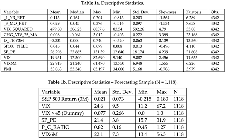
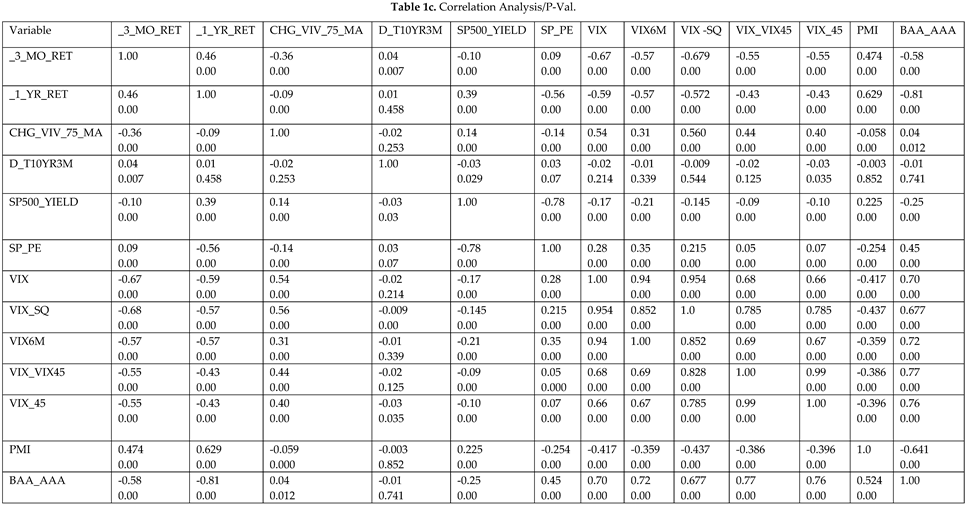
Table 1a reports descriptive statistics for ten variables across 4,342 daily observations, including returns, implied volatility, valuation ratios, and macro-financial proxies. VIX and VIX_SQUARED show high skewness and kurtosis, signaling asymmetric tail risk. Table 1b presents the 1,118-observation forecasting dataset used in logistic and OLS models. Table 1c shows the predictor correlation matrix. These statistics guide model specification by highlighting structural patterns, particularly in volatility-sensitive variables relevant for return forecasting.
Table 1c displays correlation coefficients with associated t-statistics and p-values across 4,342 observations, revealing critical relationships among financial and macro variables. VIX measures are negatively correlated with S&P 500 returns, consistent with the inverse volatility-return relationship. Forward returns correlate positively with macro indicators, while the S&P 500 yield is inversely related to returns. The term spread’s first difference is also negatively correlated with returns, reinforcing its role in signaling monetary shifts and justifying inclusion in forecasting models.
4.1. 2SLS Regression: Forward Returns Following VIX Spikes
The regression analysis predicts three-month forward returns, with VIX significantly negatively related to returns. The interaction term (VIX_45 × VIX) is also significant, suggesting diminishing marginal effects of extreme volatility spikes. Notably, VIX_45 remains economically meaningful despite marginal significance. One-year 2SLS regressions mirror these patterns, showing a highly significant and negative coefficient for VIX_45 (−23, p = 0.008), indicating that extreme implied volatility levels predict lower future returns. However, intermediate volatility (VIX6M) correlates positively with future returns, implying horizon-dependent return patterns across the volatility curve. Table 2’s 2SLS specifications confirm that VIX consistently predicts lower short-term equity returns, supporting Hypothesis 1. The nonlinear relationship is captured through interaction and threshold-based terms, which improve modeling of volatility-return dynamics. Overall, extreme volatility spikes serve as powerful predictive signals for future returns, particularly when segmented by time horizon, offering tactical insight for both short-term caution and long-term contrarian strategies.
Volatility variables are significant and negative.
- VIX: strong negative effect during non-extreme regimes. As VIX increases, 3-month returns fall. Supports VIX as a fear gauge.
- VIX*VIX_45: Significant interaction term. Suggests that when in extreme regimes (VIX > 45), the marginal impact of VIX on returns becomes less negative — implying desensitization to fear once panic is fully priced.
- VIX6M: Significant and positive. Suggests that higher 6-month implied volatility forecasts higher future returns — possibly a sign of mean reversion or a risk premium.
Control variables also perform as expected:
- SP_PE (valuation): Highly significant and positive. Higher P/E ratios are associated with higher 3-month returns. This may suggest momentum or optimism in valuation persists in the short term.
- SP500 Yield: Not significant at 5%. Suggests higher dividend yields may (unexpectedly) predict lower future returns, but the result is weak. It could reflect risk aversion.
- R-sq: Not a meaningful metric in 2SLS with HAC errors; can be negative and unreliable
Newey–West HAC standard errors were used to confirm the robustness of regression estimates, addressing serial correlation and heteroskedasticity common in financial return series. Despite occasional negative R² values from the 2SLS estimation under HAC, key predictors, especially those tied to implied volatility, remained statistically significant. Adjusted R² values ranged from 0.12 to 0.19, indicating moderate explanatory power. The Durbin–Watson test confirmed positive autocorrelation, validating the need for correction. Figure 1 visually supports model performance, showing actual vs. predicted three-month returns across normal and high-stress market periods.
4.1.1. Model Accuracy Metrics
The 2SLS model demonstrates moderate predictive accuracy. RMSE (0.0836) and MAE (0.0611) exceed those of the GARCH model, indicating less precise forecasts. MAPE (277.79%) and SMAPE (104.72%) are inflated due to near-zero returns skewing percentage-based metrics. However, Theil’s U (0.517) shows improvement over a naive forecast. Decomposition reveals a higher bias proportion (0.168), minimal variance error (0.004), and a dominant covariance proportion (0.827), indicating most errors stem from timing mismatches—typical in macro-financial forecasting—rather than magnitude misestimation.
4.1.2. Practical Interpretation
The 2SLS model (Table 2) proves more effective at aligning with return variance (volatility magnitude) but falls short in minimizing forecast bias and absolute error compared to the GARCH model. Most forecast discrepancies stem from temporal misalignment—correctly predicting the direction and size of moves but missing the timing. This characteristic is well-known in financial markets and underscores the difficulty of timing stress events. However, the model's utility is still relevant for practitioners: the confidence bands around point forecasts can aid risk managers in scaling positions based on expected return dispersion and uncertainty.
Bottom Line:
- GARCH Models yield more accurate point forecasts, lower bias, and better overall tracking.
- 2SLS excels in capturing volatility magnitude but suffers from systematic bias and larger average errors.
4.1.3. Endogeneity Assessment7
To test for endogeneity, a Durbin–Wu–Hausman test using the difference-in-J-statistic was conducted within the 2SLS framework. The test returned a J-statistic of 8.02 × 10⁻³⁹ with zero degrees of freedom, implying identical restricted and unrestricted models. Thus, exogeneity could not be rejected, and 2SLS was unnecessary. The model was re-estimated using OLS with Newey–West HAC errors, improving efficiency and interpretability while maintaining robustness. This reflects a data-driven shift to OLS as the more appropriate specification.
Table 3 presents OLS regression results using Newey–West standard errors to ensure robustness against autocorrelation and heteroskedasticity. The VIX_45 variable is significantly negative, reinforcing that extreme volatility predicts lower near-term returns. SP_PE shows a marginally positive effect, suggesting elevated valuations may signal market optimism under certain conditions. These findings align with the 2SLS results and highlight the predictive importance of volatility shocks and valuation sentiment in forecasting three-month S&P 500 returns.
Table 3b shows the model performs moderately well in stable periods but falters during volatility spikes and market stress, as Figure 1 illustrates. Forecast errors widen in high-uncertainty regimes driven by sudden changes in sentiment or implied volatility. These limitations expose the challenge of modeling tail-risk environments using linear frameworks. Even with HAC standard errors, the model's structure lacks resilience under stress, suggesting regime-switching or non-linear methods may improve predictive performance in turbulent conditions.
4.2. Logistic Regression Results
This section reports results from a logistic regression estimating the likelihood of near-term extreme volatility, defined as VIX > 45. The binary dependent variable captures these rare events, while predictors include valuation ratios, credit spreads, implied volatility term structures, and sentiment proxies. Enhancements based on robustness checks introduce interaction terms and transformed variables. Model performance is evaluated using standard classification metrics and benchmarked against a naïve baseline to assess its added forecasting value. The regression specification is as follows:
where logit⁻¹(x) = 1 / (1 + exp(-x)) is the inverse logit function.
Pr(VIX_t > 45) = logit⁻¹(20.7046 + 2.9236 × _3_MO_RET_t - 124.0313 × SP500_YIELD_t - 0.1219 × SP_PE_t + 0.8657 × VIX6M_t - 8.3441 × BAA_AAA_t + 3.0657 × P_C_RATIO_t)
All coefficients are estimated using maximum likelihood with robust standard errors (Huber-White).
Table 3 reports logistic regression results for predicting extreme volatility (VIX > 45). Valuation and sentiment indicators are significant predictors: the SP_PE ratio is positively signed (p < 0.01), and the put-call ratio (P_C_RATIO) is also positive (p < 0.05), supporting behavioral interpretations of elevated hedging activity. VIX6M and lagged returns (RETₜ₋₁) are not statistically significant. The model attains a McFadden R² of 0.38 and correctly classifies 89% of cases, demonstrating the utility of combining valuation and sentiment metrics in forecasting tail-risk volatility episodes.
The model is a binary event; the coefficient interpretation should be in terms of the effect on the log-odds (and probability) of observing a VIX spike:
Therefore, we interpret the log-odds as follows:
| Variable | Interpretation (Adjusted for Binary DV) |
| VIX6M | A 1-unit increase in the 6-month implied volatility increases the log-odds that VIX > 45. Since the coefficient is positive and significant, this means a higher VIX6M is strongly associated with a greater probability of entering a panic regime. |
| SP_PE | A 1-unit increase in the S&P 500 P/E ratio decreases the probability of VIX > 45. This suggests optimism in valuation correlates with lower panic risk. |
| P_C_RATIO | A higher put/call ratio increases the odds of a VIX spike. This reflects investor hedging behavior or fear, signaling an elevated risk of regime transition. |
| BAA_AAA | The negative coefficient means a wider credit spread (i.e., worsening credit sentiment) is surprisingly associated with a lower probability of VIX > 45, which could reflect a flight-to-quality effect — when equities crash, high-grade bond spreads may widen after the initial equity panic, not before. |
Table 4 shows that the 3-month forward return lacks statistical significance in predicting VIX spikes, consistent with theory—future returns should not influence current volatility. This affirms Hypothesis 2, which identifies valuation (SP_PE, credit spreads, S&P 500 yield) and sentiment (put-call ratio) as significant drivers of extreme volatility. Notably, the positive, significant effect of P_C_RATIO highlights its behavioral role, indicating that heightened hedging demand often precedes tail-risk events, aligning with investor expectations of adverse market conditions.
Figure 2 illustrates the marginal effects from the logistic model estimating VIX > 45. The S&P 500 Yield exerts a strong negative effect, reinforcing its stabilizing role. VIX6M, by contrast, contributes modestly and positively, suggesting medium-term volatility adds incrementally to the likelihood of extreme market stress.
Figure 3 visualizes the nonlinear link between VIX6M and the probability of VIX > 45. As VIX6M exceeds 40, the probability sharply accelerates toward 1.0, signaling elevated medium-term volatility as a key early warning indicator of tail risk for volatility-sensitive investors and portfolio risk managers.
4.3. GARCH Regression Results
Table 5 reports GARCH (1,1) results for 1-year (Model A) and 3-month (Model B) return forecasts. Both exhibit excellent in-sample fit (R²: 0.9949 and 0.9779, respectively). SPX_TR is highly significant in the variance equation (p = 0.000), and GARCH(1) terms above 0.85 confirm volatility persistence. Residual diagnostics show no serial correlation. While both models are stable, Model B’s lower AIC/BIC indicates marginally greater efficiency for short-horizon return prediction.
4.3.1. Conditional Volatility and Return Forecasting Using GARCH Models
To further assess the dynamic structure of equity-return volatility, we estimate Generalized Autoregressive Conditional Heteroskedasticity (GARCH) models for both short-term (3-month) and longer-term (1-year) forward return forecasts. These models are well-suited to capture volatility clustering and time-varying risk, which are prevalent in financial time series.
4.3.2. 3-Month Return GARCH (1,1) Model.
The GARCH (1,1) specification for 3-month forward returns captures conditional heteroskedasticity in residuals from the baseline linear model. Results indicate the following:
- ARCH (1) = 0.1201, positive and statistically significant. This suggests that approximately 12% of current conditional volatility is explained by the most recent return shock, reflecting a moderate short-term reaction to market surprises.
- GARCH (1) = 0.8628, also highly significant, denotes strong persistence in volatility. Once a volatility spike occurs, it decays slowly.
- The sum of ARCH (1) and GARCH (1) equals 0.982978, a value remarkably close to 1. This indicates a highly persistent volatility process and confirms the presence of volatility clustering, consistent with prior empirical finance literature.
This model thus supports the notion that equity market volatility in the short term is slow to mean-revert, with risk lingering after initial shocks. The model’s accuracy metrics, as discussed earlier, further confirm its superior forecasting capability compared to the 2SLS alternative.
4.3.3. 1-Year Return GARCH (1,1) Model
Extending the horizon, we estimate a comparable GARCH (1,1) model for one-year forward returns. The results mirror the findings from the 3-month model but display even greater persistence:
- ARCH (1) = 0.1322, statistically significant, indicates that about 13% of the change in current volatility is driven by recent return innovations.
- GARCH (1) = 0.8569, again highly significant, reflects extremely strong persistence. This suggests that periods of high volatility at the annual level are likely to remain elevated over extended durations.
- The ARCH (1) + GARCH (1) = 0.9891, further confirms the extreme persistence and slow mean reversion of conditional volatility. This near-unit root behavior indicates that volatility regimes, once entered, are likely to be sustained.
4.3.4. Interpretation and Implications
In both GARCH models, the sum of the ARCH and GARCH terms is close to 1, indicating that volatility shocks dissipate slowly, reinforcing the need for risk management models to account for volatility clustering (Figure 4).
- In the short horizon, recent shocks matter, but long-run persistence dominates.
- In the long horizon, volatility is even more “sticky,” suggesting the market retains “memory” of past risk levels.
Strong GARCH effects confirm that market volatility is time-varying and path-dependent, validating the use of conditional variance models for asset allocation and stress testing. These results support Hypothesis 3, affirming that time-varying risk models like GARCH offer meaningful forward-looking insight into evolving volatility regimes.
Model A (1-year GARCH) delivers superior long-term forecast precision, explaining significant return variance with lower standard error. High volatility persistence (ARCH = 0.1322, GARCH = 0.8569) reflects strong clustering and slow mean reversion, consistent with empirical patterns. Model B, while equally precise, achieves lower AIC/BIC values, favoring parsimony at a shorter horizon. Both models include AR(1) and MA(1) terms, yielding well-specified residuals—supported by Durbin–Watson statistics near 2.0. Notably, both models exhibit similar responses to volatility shocks, reinforcing their robustness and reliability across distinct return intervals and macro-financial regimes.
Table 6 reveals that most explanatory variables are statistically significant, underscoring the role of volatility and valuation in shaping forward returns. The squared VIX term is notably significant, supporting a nonlinear volatility-return relationship consistent with behavioral finance theory. In contrast, the VIX_45 dummy is insignificant, suggesting threshold breaches lack standalone predictive power. Macroeconomic indicators like PMI and credit spreads also show limited relevance, potentially reflecting the market’s evolving focus on real-time sentiment measures. Collectively, these findings support the hypothesis that continuous volatility metrics offer greater explanatory power than binary indicators, emphasizing the importance of modeling nonlinear dynamics in forecasting short-term equity returns.
Table 7 shows that short-term equity returns are primarily driven by implied volatility, particularly the VIX_45 indicator and its interaction term, supporting Hypothesis 1’s behavioral foundation. In contrast, macroeconomic variables like PMI and credit spread are statistically insignificant, suggesting limited short-horizon relevance. The lone exception is the change in the 10Y–3M spread, which shows modest predictive value. These findings affirm that sentiment-based measures dominate short-run return dynamics, while economic indicators are more influential over longer horizons.
4.4. Out-of-Sample Results
To evaluate the robustness and predictive validity of the regression framework, we extend the analysis through an out-of-sample forecasting exercise using updated Two-Stage Least Squares (2SLS) models. This step is essential for assessing the model’s generalizability beyond the estimation window and gauging its practical utility in forecasting future equity returns.
4.4.1. Baseline Forecast Model
The first model iteration employs traditional predictors, including lagged S&P 500 returns and fundamental valuation metrics. As shown in Figure 3, this specification captures the general directional trend of S&P 500 three-month forward returns with a reasonably high adjusted R². While deviations are observed around market inflection points, the model exhibits satisfactory directional accuracy, providing initial evidence of out-of-sample effectiveness.
4.4.2. Enhanced Model with Macro-Volatility Indicators
We then introduce a second model specification, expanding the set of predictors to include the term spread (T10Y3M) and a nonlinear volatility term (VIX²). These enhancements aim to better capture forward-looking macro-financial stress and volatility clustering, two factors often omitted in standard linear models 8,9. As illustrated in Figure 4, the enhanced model demonstrates improved alignment with realized return trajectories and a notable reduction in forecast error variance. The term spread increases the model's sensitivity to recessionary signals, while the squared VIX term provides a correction for nonlinear and persistent shifts in market uncertainty.
4.4.3. GARCH-Based Out-of-Sample Forecast
Complementing the 2SLS results, the GARCH (1,1) model forecasts three-month returns by dynamically modeling volatility. As shown in Figure 5, it captures both the amplitude and persistence of return fluctuations across calm and turbulent periods. Out-of-sample performance demonstrates close alignment with realized returns, supporting the model’s predictive validity. These findings highlight the value of integrating behavioral indicators, valuation ratios, and macro-volatility signals into a multi-layered forecasting framework tailored for complex financial environments.
Key accuracy metrics:
- RMSE = 0.0583 and MAE = 0.0441 → errors are relatively small in absolute terms.
- MAPE ≈ 170.88% and SMAPE ≈ 88.16% → large % errors occur because many returns are near zero, so even small deviations inflate these metrics.
- Theil’s U = 0.435 → below 1, meaning the model beats a naive “no-change” forecast.
- Bias proportion (0.033) is low → no strong tendency to over- or underpredict.
- Variance proportion (0.426) is moderate → some mismatch in volatility magnitude.
- Covariance proportion (0.541) is moderate → errors also come from timing mismatches between predicted and actual peaks/troughs.
Performance metrics:
- RMSE = 0.1488 and MAE = 0.1263 → average forecast errors in absolute terms are moderate.
- MAPE ≈ 461% and SMAPE ≈ 96.95% → percentage errors are remarkably high because returns are often close to zero, so even small misses inflate percentage metrics.
- Theil U = 0.410 → values < 1 mean the model beats a naive “no-change” forecast; here, it is decent.
- Bias proportion (0.03) is low → forecasts are not systematically too high or too low.
- Variance proportion (0.11) is low → model matches the magnitude of fluctuations fairly well.
- Covariance proportion (0.86) is high → most error is from timing mismatches (model gets the size right but not the exact timing of peaks/troughs).
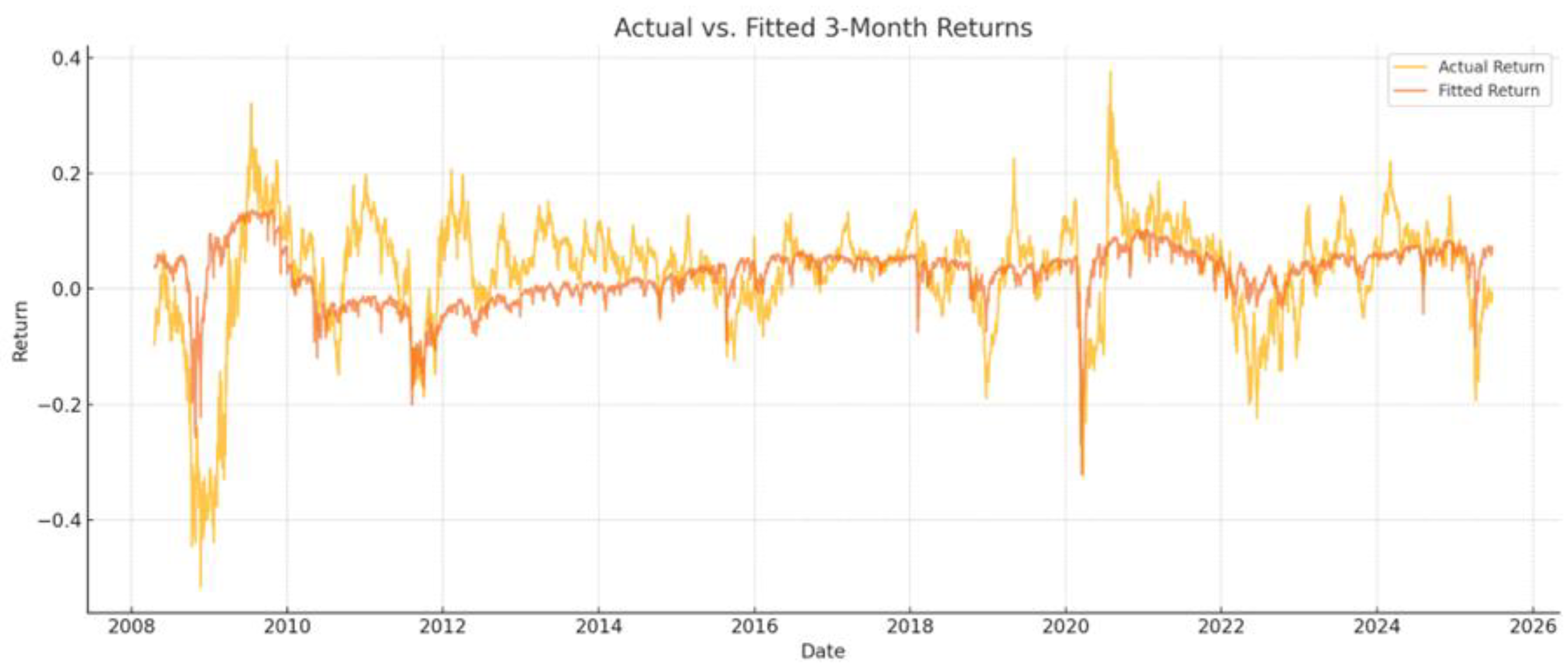
The graph (Figure 6) presents actual S&P 500 returns against the forecasted returns generated by the model using traditional variables, while Figure 7 presents the Forecasted Returns against the Actual Returns Out-of-Sample. The model shows strong trend-capturing performance despite some timing errors present.
The enhanced model (Figure 8), integrating the T10Y3M term spread and squared VIX (VIX²), improves out-of-sample accuracy by reducing error variance and tracking realized returns more closely. These macro-volatility proxies enhance sensitivity to systemic risk and nonlinear dynamics. Table 8 confirms improved predictive precision under stress, supporting Hypothesis 3. The model outperforms traditional benchmarks by blending valuation, sentiment, and macroeconomic indicators demonstrating the strength of multi-dimensional forecasting in capturing market complexity.
4.5. Summary of Findings
This section integrates findings from the volatility and return prediction models in Section 4.1, Section 4.2, Section 4.3 and Section 4.4, affirming the role of behavioral and macro-financial indicators in shaping equity dynamics. Elevated implied volatility, particularly VIX spikes, is linked to negative excess returns, reinforcing their value as leading signals. OLS and logistic models demonstrate predictive strength when incorporating sentiment, valuation, and volatility inputs, while GARCH-based models show limitations during nonlinear risk shifts. However, regime-specific thresholds like VIX > 45 offer incremental predictive value.
Enhanced GARCH (1,1) models validate Hypothesis 1 by exhibiting volatility clustering (ARCH + GARCH ≈ 0.98–0.99), with lagged returns and valuation ratios improving conditional variance forecasts. Logistic regressions support Hypothesis 2, showing that the likelihood of extreme volatility rises with higher VIX6M, elevated SP_PE, and the put-call ratio. Classification accuracy reaches 89%, with McFadden R² = 0.38. The insignificance of forward returns aligns with theoretical expectations that future outcomes do not influence current volatility.
Updated 2SLS models confirm Hypothesis 3, as the inclusion of the T10Y3M spread and VIX² significantly improves R², RMSE, and MAE. These terms capture nonlinear volatility dynamics and liquidity risk often missed in linear models. Collectively, the results highlight that combining behavioral, valuation, and macro-volatility measures enhances return forecasting under systemic stress and supports a robust multi-factor modeling approach.
5. Implications for Theory and Practice
This research carries important implications for financial theory and investment practice. The observed predictive power of VIX² and the T10Y3M term spread supports core tenets of risk-based asset pricing, extending frameworks such as Campbell and Shiller (1988) and Lettau and Ludvigson (2001), which emphasize time-varying risk premia and conditional expected returns. Nonlinear volatility metrics act as proxies for investor uncertainty, while the term spread reinforces the macro-financial link to risk compensation.
Robustness across OLS, logistic regression, and GARCH (1,1) models highlights the importance of regime-sensitive and higher-moment risk factors. These results encourage hybrid approaches that blend econometrics with machine learning to detect nonlinearities and structural breaks.
For practitioners, enhanced models that integrate VIX², term spreads, and valuation ratios enable more adaptive, risk-aware portfolio construction. VIX6M and the put-call ratio prove particularly valuable for tail-risk hedging, stress monitoring, and volatility-triggered signals. Institutional strategies, hedge funds, risk-parity, and tactical asset allocators, can dynamically adjust exposure based on these macro-sentiment indicators.
Moreover, the evidence that nonlinear terms outperform linear models during crises underscores the need for probabilistic tools that capture drawdown risk. As financial data becomes increasingly real-time, responsive forecasting systems are now viable. Future research should expand on these results with sentiment analytics, microstructure data, and alternative signals. In sum, multifactor frameworks offer a powerful lens for navigating modern market dynamics.
5.1. Discussion
The empirical models developed in this study exhibit strong predictive power and theoretical grounding, yet several limitations merit further exploration. Forecasting accuracy is contingent on the stability of input variables such as VIX, VIX6M, and PMI, indicators prone to revision, sampling distortions, and structural breaks. Model robustness may thus deteriorate during atypical regimes or macroeconomic shocks.
Transformations like squared volatility terms and moving averages helped capture nonlinear dynamics but risk overfitting during dislocations. While OLS and logistic regressions offer interpretability, they assume stable relationships, which may falter amid crises or shifts in market structure. GARCH (1,1) models improved short-term volatility tracking but exhibited limited adaptability across cycles. Future research should consider enhancements such as rolling estimations or regime-switching mechanisms.
Geographically, this study is U.S.-centric, limiting generalizability. Term spreads and volatility indices may behave differently across markets due to policy divergences and liquidity conditions, necessitating localized model recalibration for global application.
Moreover, machine learning and nonparametric methods were not explored, though they may capture hidden interactions or nonlinearities missed by classical approaches. These tools could support improved tail-risk prediction and threshold-triggered regime modeling.
Lastly, practical constraints like transaction costs, liquidity frictions, and rebalancing overhead remain unmodeled. Despite statistical gains, real-world efficacy depends on net risk-adjusted returns.
In sum, this study provides a foundation for integrating behavioral, valuation, and macro-financial indicators into a cohesive forecasting framework, offering opportunities for refinement, broader datasets, and actionable investment applications.
5.2. Conclusion
This study contributes new empirical evidence and theoretical insight into the role of volatility-sensitive and macro-financial indicators in forecasting equity returns and detecting shifts in market risk regimes. By incorporating forward-looking variables—specifically the squared VIX (VIX²), the six-month implied volatility index (VIX6M), and the term spread (T10Y3M)—the models developed herein offer substantial explanatory power over future market conditions.
Using logistic regression, OLS, and GARCH-based models, the analysis shows enhanced predictive accuracy, particularly during volatile periods. Nonlinear transformations and moving average filters further improve performance by capturing regime-dependent behavior and reducing model instability under stress. These enhancements allow for better identification of market dynamics that traditional linear approaches may overlook.
The findings challenge assumptions underlying the Efficient Market Hypothesis (EMH), particularly the notion that returns cannot be forecasted using public information. Consistent with behavioral finance and macro-based asset pricing literature, the results validate multi-factor models that blend theoretical constructs with sentiment and volatility measures to improve risk-adjusted performance.
Practically, the study offers meaningful insights for portfolio managers, asset allocators, and policymakers. The consistent predictive strength across models and timeframes underscores the importance of incorporating volatility and macro-financial variables into forecasting frameworks. These results support the development of adaptive, risk-aware allocation strategies that are more responsive to evolving market conditions. Ultimately, the research bridges theoretical modeling and applied finance, providing a foundation for future studies to explore hybrid techniques that integrate econometric rigor with machine learning and alternative data.
| 1 | Whaley (2000) coined the VIX as a "fear gauge." Bekaert & Hoerova (2014) empirically linked VIX levels to investor risk aversion via the variance risk premium. |
| 2 | A substantial literature has examined the VIX and its role as a barometer of investor fear, emphasizing its capacity to capture market sentiment and perceived risk (Whaley, 2000; Fleming, Ostdiek, & Whaley, 1995; Smales, 2014). |
| 3 | Observable market signals, including lagged negative returns, heightened realized volatility, and deteriorating investor sentiment, have been shown to precede sharp increases in implied volatility (Blair, Poon, & Taylor, 2001; Andersen et al., 2003; Smales, 2017). |
| 4 | Hamilton & Susmel (1994) introduce regime-switching in volatility models as a response to GARCH limitations during instability. Ang & Bekaert (2002) model regime changes and show that traditional GARCH models often miss these shifts. Andersen et al. (2007) incorporate jumps and discontinuities into volatility forecasting, showing superior performance in turbulent environments. |
| 5 | The CBOE S&P 500 6-Month Volatility Index SM (Ticker: VIX6M) is an estimate of the expected 6-month volatility of the S&P 500® Index. It is calculated using the well-known VIX methodology applied to SPX options that expire 6-to-9 months in the future. |
| 6 | RMSE captures the magnitude of forecast errors and emphasizes large deviations, which is critical in volatility forecasting. SMAPE normalizes the error relative to scale and treats over- and underestimations symmetrically, helpful when volatility levels vary. Theil’s U² benchmarks model forecasts against naïve benchmarks like a random walk; values < 1 indicate improvement over that simple approach. (Buturac, G. (2022)., Bekaert, G., & Hoerova, M. (2014). |
| 7 | A similar process was conducted on the 1-year return 2SLS, and the variables were all exogenous. |
| 8 | While VIX² is widely accepted as a forward-looking measure of market volatility and liquidity stress, the T10Y3M spread (10-Year Treasury minus 3-Month Treasury yield) is not a direct measure of liquidity risk, but it can serve as a leading indicator of systemic financial and macroeconomic stress, which often coincides with or precedes liquidity crises. Adrian, T. and Shin, H.S. (2010), Brunnermeier & Pedersen (2009). |
| 9 | The square of the VIX index → measures option-implied variance of S&P 500 returns. Market makers widen spreads or withdraw due to the risk of adverse selection. Investors become reluctant to trade — particularly large blocks. Brunnermeier & Pedersen (2009). |
References
- Adrian, T. and Shin, H.S., "Liquidity and Leverage," Journal of Financial Intermediation 19, no. 3 (July 2010): 418–37.
- Andersen, T. G., Bollerslev, T., Diebold, F. X., & Vega, C. (2003). Micro effects of macro announcements: Real-time price discovery in foreign exchange. American Economic Review, 93(1), 38–62. [CrossRef]
- Andersen, T. G., Bollerslev, T., & Diebold, F. X. (2007). Roughing it up: Including jump components in the measurement, modeling, and forecasting of return volatility. Review of Economics and Statistics, 89(4), 701–720. [CrossRef]
- Ang, A., & Bekaert, G. (2002). Regime switches in interest rates. Journal of Business & Economic Statistics, 20(2), 163–182. [CrossRef]
- Baker, M., & Wurgler, J. (2007). Investor sentiment in the stock market. Journal of Economic Perspectives, 21(2), 129-151.
- Bali, T. G., & Zhou, H. (2016). Risk, uncertainty, and expected returns. Journal of Financial and Quantitative Analysis, 51(3), 707–735.
- Barberis, N., Shleifer, A., & Vishny, R. (1998). A model of investor sentiment. Journal of Financial Economics, 49(3), 307–343.
- Barberis, N., & Thaler, R. (2003). A survey of behavioral finance. In G. M. Constantinides, M. Harris, & R. M. Stulz (Eds.), Handbook of the economics of finance (Vol. 1, pp. 1053–1128). Elsevier. [CrossRef]
- Black, F. (1976). Studies of stock price volatility changes. In Proceedings from the American Statistical Association, Business and Economic Statistics Section (p. 177).
- Blair, B. J., Poon, S. H., & Taylor, S. J. (2001). Forecasting S&P 100 volatility: the incremental information content of implied volatilities and high-frequency index returns. Journal of Econometrics, 105(1), 5–26.
- Bekaert, G., & Hoerova, M. (2014). The VIX, the variance premium, and stock market volatility. Journal of Econometrics, 183(2), 181-192.
- Blitz, D., van Vliet, P., & Baltussen, G. (2019). When equity factors drop their shorts. Journal of Portfolio Management, 45(6), 35–49. [CrossRef]
- Bollerslev, T., Tauchen, G., & Zhou, H. (2009). Expected stock returns and variance risk premia. The Review of Financial Studies, 22(11), 4463-4492.
- Bollerslev, T., Todorov, V., & Xu, L. (2015). Tail risk premia and return predictability. Journal of Financial Economics, 118(1), 113-134.
- Bollerslev, T. (1986). Generalized autoregressive conditional heteroskedasticity. Journal of Econometrics, 31(3), 307–327. [CrossRef]
- Brunnermeier, M. K., & Pedersen, L. H. (2009). Market Liquidity and Funding Liquidity. The Review of Financial Studies, 22(6), 2201–2238. http://www.jstor.org/stable/30225714.
- Buturac, G. (2022). Measurement of forecast accuracy and economic interpretation: An overview of frequently used metrics. Journal of Risk and Financial Management, 15(1), 1. [CrossRef]
- Cameron, A. C., & Miller, D. L. (2015). A Practitioner’s Guide to Cluster-Robust Inference. Journal of Human Resources, 50(2), 317–372. [CrossRef]
- Campbell, J. Y., & Hentschel, L. (1992). No news is good news: An asymmetric model of changing volatility in stock returns. Journal of Financial Economics, 31(3), 281–318.
- Campbell, J. Y., & Shiller, R. J. (1988). The dividend-price ratio and expectations of future dividends and discount factors. The review of financial studies, 1(3), 195–228.
- Cboe Global Markets, Inc. (n.d.). Cboe Volatility Index (VIX). Retrieved July 25, 2025, from https://www.cboe.com/tradable_products/vix/.
- Chief Investment Office. (2025, April). Eyes on the road ahead (Volatility Charts Report). Merrill Lynch, Pierce, Fenner & Smith Incorporated. https://mlaem.fs.ml.com/content/dam/ML/ecomm/pdf/MV_Chartbook_Merrill.pdf.
- Chief Investment Office. (2025, April 23). The climb back: What past downturns tell us about the road to recovery. Merrill Lynch, Pierce, Fenner & Smith Incorporated. https://www.merrilledge.com/article/managing-market-downturns-volatility#climb-back.
- Christoffersen, P. F., & Diebold, F. X. (2006). Financial asset returns, direction-of-change forecasting, and volatility dynamics. In G. T. Dewaelheyns & L. E. O. Svensson (Eds.), Directions in financial econometrics and statistics (pp. 1–27). Springer. [CrossRef]
- Cochrane, J. H. (2005). Asset pricing (Rev. ed.). Princeton University Press.
- Daniel, K., Hirshleifer, D., & Subrahmanyam, A. (1998). Investor psychology and security market under-and overreactions. the Journal of Finance, 53(6), 1839-1885.
- De Bondt, W. F. M., & Thaler, R. H. (1985). Does the stock market overreact? Journal of Finance, 40(3), 793–805. [CrossRef]
- DeBondt, W. F. M., & Richard H. Thaler (1995). Financial decision-making in markets and firms: A behavioral perspective; in Robert A. Jarrow, Vojislav Maksimovic, and William. Ziemba, eds.: Finance, Handbooks in Operations Research and Management Science 9,385-410 (North Holland, Amsterdam).
- Drechsler, I., & Yaron, A. (2011). What's vol got to do with it. The Review of Financial Studies, 24(1), 1-45.
- Engle, R. F. (1982). Autoregressive conditional heteroscedasticity with estimates of the variance of United Kingdom inflation. Econometrica, 50(4), 987–1007. [CrossRef]
- Fleming, J., Kirby, C., & Ostdiek, B. (2003). The economic value of volatility timing using “realized” volatility. Journal of Financial Economics, 67(3), 473–509.
- Fleming, J., Ostdiek, B., & Whaley, R. E. (1995). Predicting stock market volatility: A new measure. Journal of Futures Markets, 15(3), 265–302. [CrossRef]
- French, K. R., Schwert, G. W., & Stambaugh, R. F. (1987). Expected stock returns and volatility. Journal of Financial Economics, 19(1), 3–29.
- Ghysels, E., Santa-Clara, P., & Valkanov, R. (2005). There is a risk-return trade-off after all. Journal of Financial Economics, 76(3), 509–548.
- Gu, S., Kelly, B., & Xiu, D. (2020). Empirical asset pricing via machine learning. The Review of Financial Studies, 33(5), 2223–2273.
- Han, B. (2008). Investor sentiment and option prices. The Review of Financial Studies, 21(1), 387–414.
- Hamilton, J. D., & Susmel, R. (1994). Autoregressive conditional heteroskedasticity and changes in regime. Journal of Econometrics, 64(1–2), 307–333. [CrossRef]
- Jegadeesh, N., & Titman, S. (1993). Returns to buying winners and selling losers: Implications for stock market efficiency. Journal of Finance, 48(1), 65–91. [CrossRef]
- Kelly, B. T., Pruitt, S., & Su, Y. (2019). Characteristics are covariances: A unified model of risk and return. Journal of Financial Economics, 134(3), 501-524.
- Kumar, A., & Lee, C. M. (2006). Retail investor sentiment and return co-movements. The Journal of Finance, 61(5), 2451–2486.
- Lettau, M., & Ludvigson, S. (2001). Consumption, aggregate wealth, and expected stock returns. the Journal of Finance, 56(3), 815-849.
- Manela, A., & Moreira, A. (2017). News implied volatility and disaster concerns. Journal of Financial Economics, 123(1), 137-162.
- Merton, R. C. (1980). On estimating the expected return on the market: An exploratory investigation. Journal of Financial Economics, 8(4), 323–361.
- Neely, C. J., Rapach, D. E., Tu, J., & Zhou, G. (2014). Forecasting the equity risk premium: The role of technical indicators. Management Science, 60(7), 1772–1791. [CrossRef]
- Newey, W. K., & West, K. D. (1987). A simple, positive semi-definite, heteroskedastic, and autocorrelation-consistent covariance matrix. Econometrica, 55(3), 703–708. [CrossRef]
- Ngoc, L. T. B. (2014). Behavior pattern of individual investors in stock market. International Journal of Business and Management, 9(1), 1–16.
- Pan, J., & Poteshman, A. M. (2006). The information in option volume for future stock prices. The Review of Financial Studies, 19(3), 871–908.
- Schwert, G. W. (1989). Why does stock market volatility change over time? Journal of Finance, 44(5), 1115–1153. [CrossRef]
- Smales, L. A. (2014). News sentiment and the investor fear gauge. Finance Research Letters, 11(2), 122–130. [CrossRef]
- Smales, L. A. (2017). The importance of fear: Investor sentiment and stock market returns. Applied Economics, 49(34), 3393–3408. [CrossRef]
- Whaley, R. E. (1993). Derivatives on market volatility. The Journal of Derivatives, 1(1), 71-84.
- Whaley, R. E. (2000). The investor fear gauge. Journal of Portfolio Management, 26(3), 12.
- Wooldridge, J. M. (2019). Introductory econometrics: A modern approach (7th ed.). Cengage Learning.
- Zhou, H. (2018). Variance risk premia, asset predictability puzzles, and macroeconomic uncertainty. Annual Review of Financial Economics, 10(1), 481-497. [CrossRef]
Figure 1.
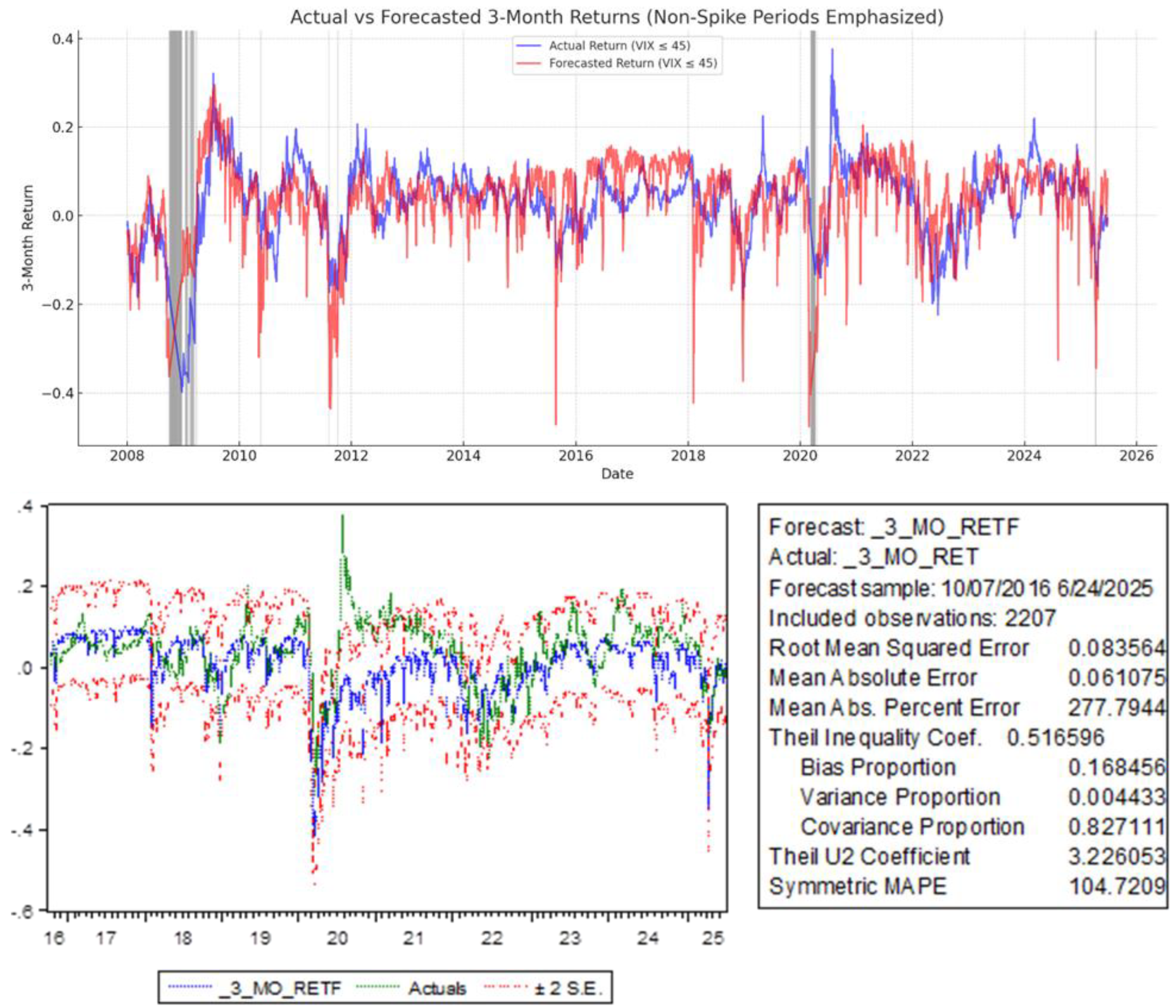
Figure 2.
Ave Marginal Effects on Pr(VIX>45).
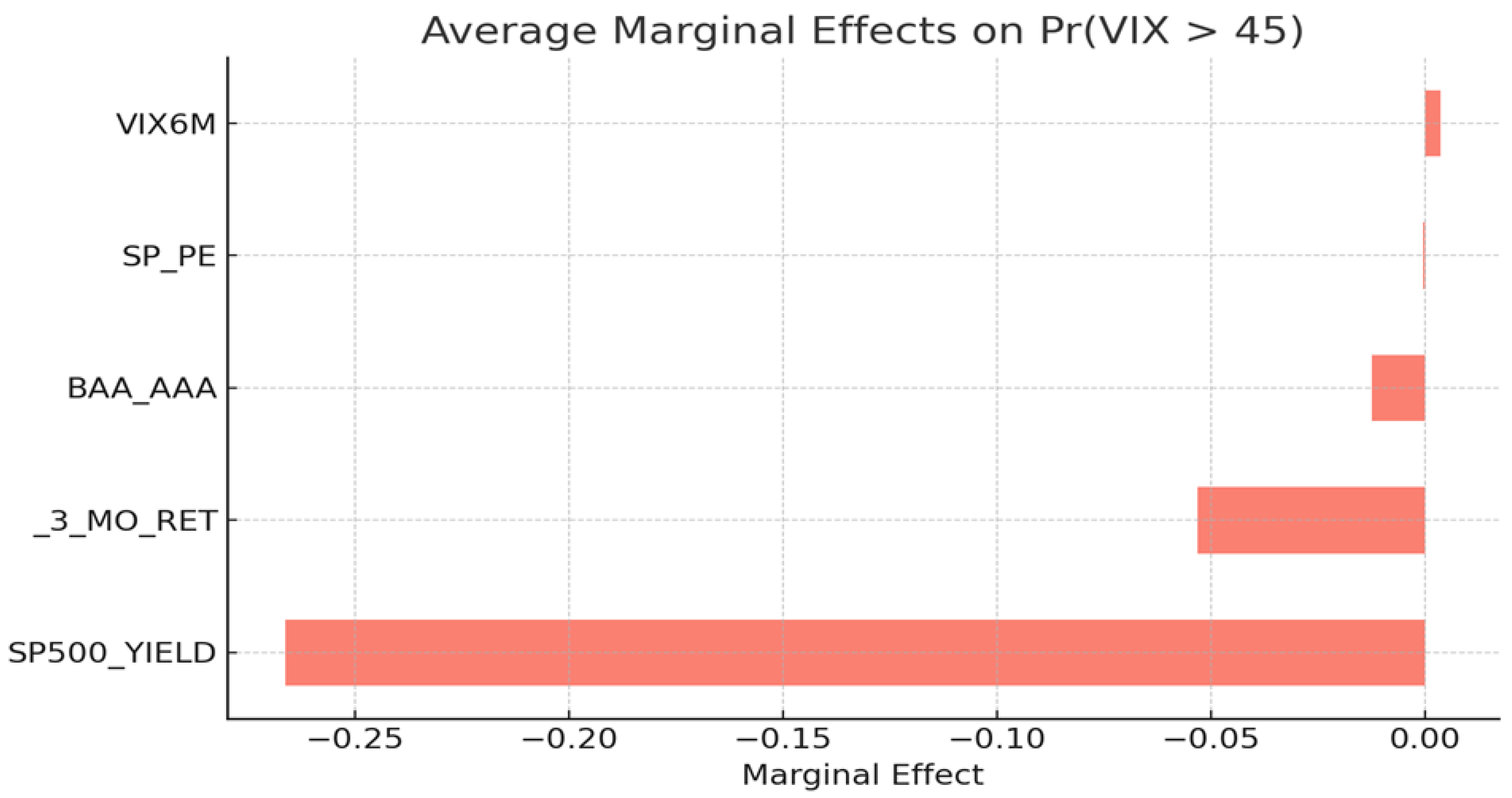
Figure 3.
Partial Dependence of Pr(VIX45) on VIX6M.
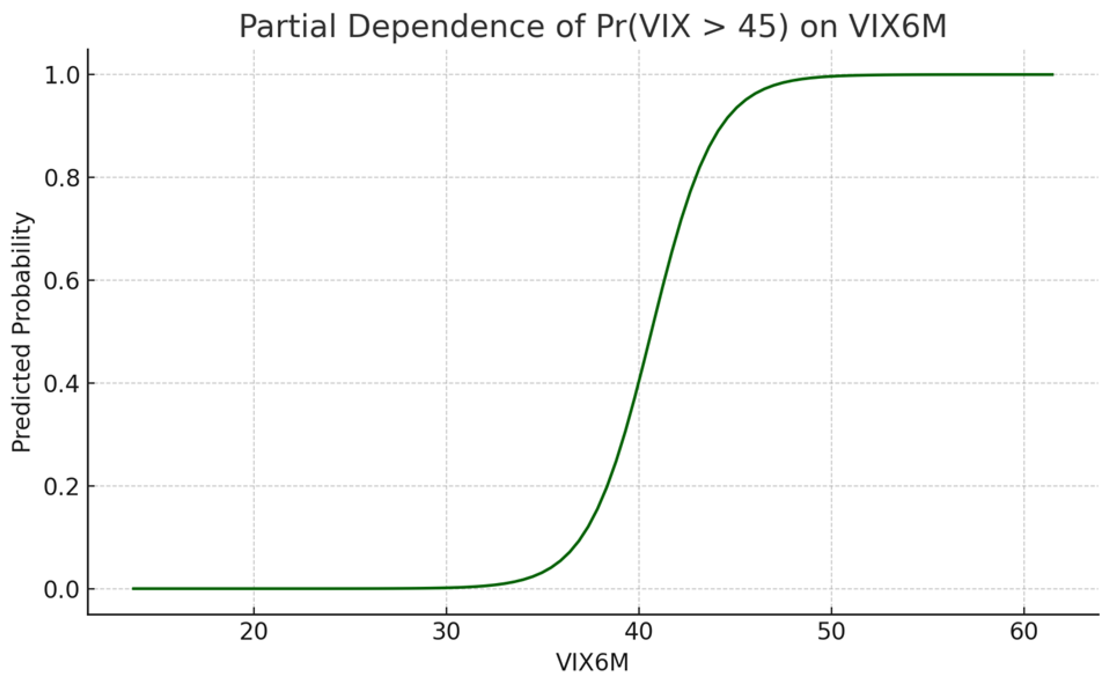
Figure 4.
GARCH (1,1) Component Comparison.
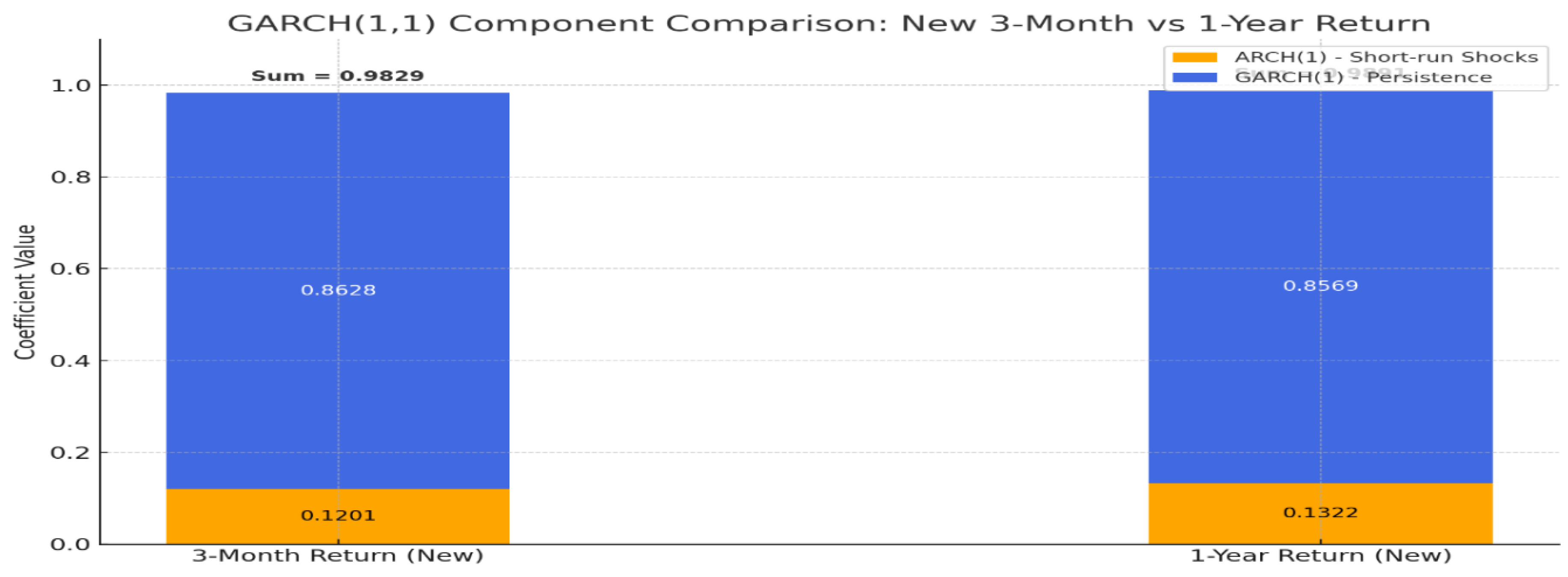
Figure 5.
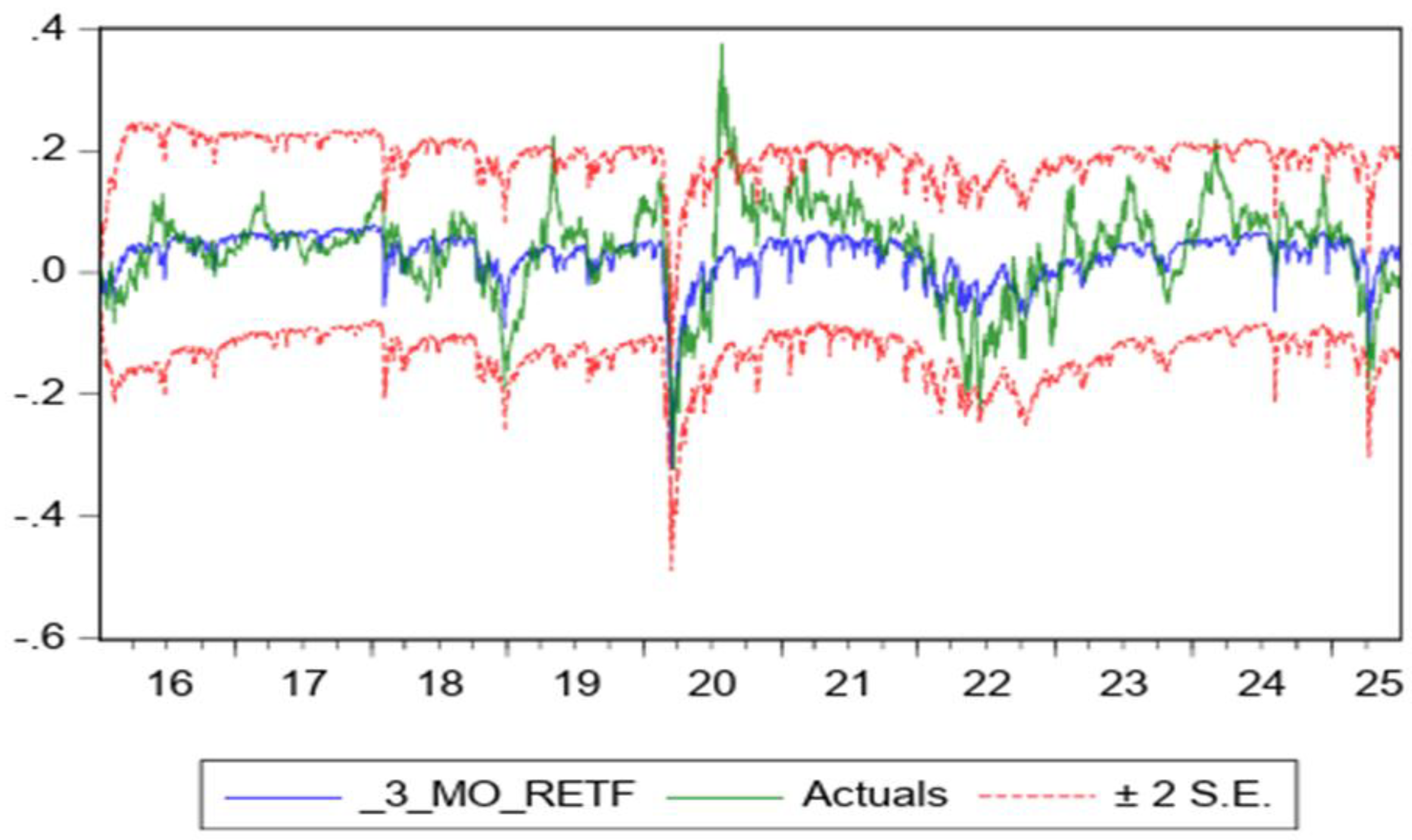
Figure 6.
Forecast vs. Actual S&P 500 Returns (1-year return GARCH (1,1) Model Out of sample data).
Figure 7.
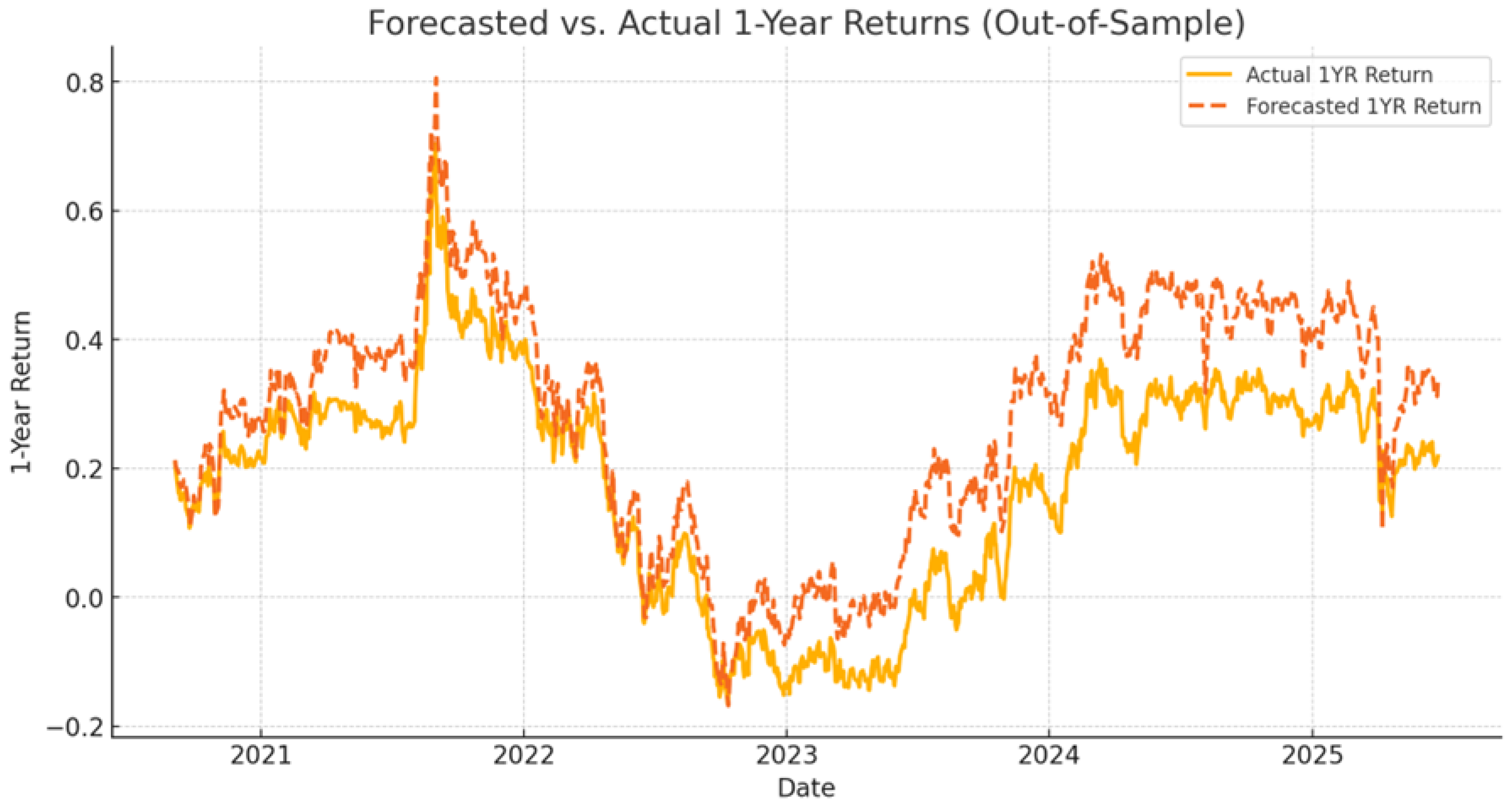
Figure 8.
Forecast vs. Actual Returns with T10Y3M spread and VIX² (Enhanced Model).

|
Table 2.
Comparative Summary: 2SLS vs. GARCH (Three-Month Horizon).
| Metric | GARCH (3M) | 2SLS (3M) | Better Model |
| RMSE | 0.0583 | 0.0836 | GARCH (3m) |
| MAE | 0.0441 | 0.0611 | GARCH (3m) |
| Bias Proportion | 0.033 | 0.168 | GARCH (3m) |
| Variance Proportion | 0.426 | 0.004 | 2SLS |
| Covariance Proportion | 0.541 | 0.827 | GARCH (3m) |
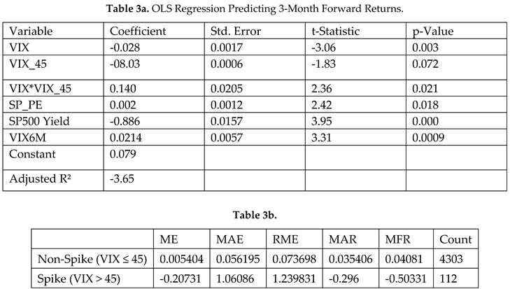 |
Table 4.
Logistic Regression Estimating Probability of VIX > 45.
| Variable | Coefficient | Std. Error | z-Statistic | P-Value |
| Intercept | 20.705 | 7.260 | 2.852 | 0.0043 |
| 3_mos ret | 2.924 | 5.622 | 0.520 | 0.603 |
| VIX6M | 0.866 | 0.203 | 4.273 | 0.000 |
| SP500__YIELD | -124.03 | 71.261 | -1.741 | 0.082 |
| SP_PE | -0.122 | 0.039 | -3.081 | 0.002 |
| BAA_AAA | -8.344 | 2.361 | -3.535 | 0.0004 |
| PMI | -0.722 | 0.186 | -3.888 | 0.001 |
| P_C_RATIO | 3.066 | 1.430 | 2.144 | 0.032 |
Note: The Dependent variable is an indicator for VIX > 45. McFadden R² = 0.85.
| Metric | Model A (_1_YR_RET) | Model B (_3_MO_RET) |
| R-squared | 0.9949 | 0.9779 |
| Adjusted R-squared | 0.9949 | 0.9778 |
| Log-likelihood | 13498.2 | 11516.5 |
| Akaike Info Criterion (AIC) | -6.1102 | -6.1185 |
| Schwarz Criterion (BIC) | -6.0870 | -6.0953 |
| S.E. of regression | 0.0144 | 0.01451 |
| Durbin-Watson | 2.0838 | 2.1102 |
| ARCH(1) | 0.1322 | 0.1201 |
| GARCH(1) | 0.8569 | 0.8628 |
| SPX_TR in Variance Eq. | Significant (p=0.000) | Significant (p=0.000) |
Table 6.
For 1 year-return dependent variable regression:.
| Variable | Coefficient | p-Value | Significance | Interpretation |
| C (Intercept) | 0.151556 | 0.4803 | Not significant | The intercept alone does not meaningfully predict 1-year returns. |
| VIX | -0.003949 | 0.0000 | Highly significant | Negative relationship: a higher VIX (fear gauge) is associated with lower future 1-year returns. |
| VIX__45 | 0.007333 | 0.4545 | Not significant | The extreme volatility regime dummy (>45) does not have an independent effect after controlling for other variables. |
| SP500__YIELD | -5.383821 | 0.0000 | Highly significant | Higher S&P 500 dividend yield predicts lower 1-year returns in this model (may indicate inverse valuation effect here). |
| SP_PE | -0.001440 | 0.0000 | Highly significant | Higher P/E ratios are associated with lower future returns — consistent with valuation mean reversion. |
| VIX_VIX45 (interaction) | -0.000379 | 0.0606 | Marginal significance | Suggests that the marginal effect of VIX is slightly more negative during extreme volatility regimes. |
| PMI | 0.000332 | 0.2491 | Not significant | Manufacturing sentiment (PMI) does not independently drive 1-year returns here. |
| BAA_AAA (credit spread) | -7.81E-05 | 0.9885 | Not significant | Credit spread changes have no significant predictive effect in this model. |
| D_T10YR3M (yield curve slope) | 0.006959 | 0.0001 | Highly significant | A steeper yield curve predicts higher future returns — consistent with recession risk signals. |
| AR (1) | 0.997768 | 0.0000 | Highly significant | Extraordinarily strong autoregressive persistence in returns — past 1-year returns heavily influence forecasts. |
| MA (1) | -0.061206 | 0.0002 | Highly significant | Negative moving-average term suggests a correction after shocks. |
Table 7.
For the 3_mos Return dependent variable regression.
| Variable | Coefficient | p-Value | Significance | Interpretation |
| C (Intercept) | 0.368840 | 0.0000 | Highly significant | Positive intercept — implies a positive baseline for 3-month returns when other variables are neutral. |
| VIX | -0.003612 | 0.0000 | Highly significant | Negative relationship: higher VIX predicts lower short-term future returns. |
| VIX__45 | 0.040017 | 0.0000 | Highly significant | Being in an extreme volatility regime (>45) is strongly associated with higher subsequent 3-month returns — consistent with rebound effects after panic. |
| SP500__YIELD | -5.616970 | 0.0000 | Highly significant | Higher dividend yield predicts lower short-term returns in this model (inverse of what is often expected — could be driven by crisis periods). |
| SP_PE | -0.001567 | 0.0000 | Highly significant | Higher P/E ratios are linked to lower short-term returns — consistent with overvaluation effects. |
| VIX_VIX45 (interaction) | -0.000905 | 0.0000 | Highly significant | In extreme volatility regimes, the marginal effect of VIX becomes more negative, dampening rebound magnitude. |
| PMI | 0.000332 | 0.1034 | Not significant | Manufacturing sentiment does not significantly explain 3-month returns here. |
| BAA_AAA (credit spread) | 0.000582 | 0.9003 | Not significant | Credit spread changes have no predictive value for short-term returns in this model. |
| D_T10YR3M (yield curve slope) | 0.003819 | 0.0367 | Significant | A steeper yield curve predicts higher 3-month returns, possibly signaling lower near-term recession risk. |
| AR (1) | 0.989649 | 0.0000 | Highly significant | Extraordinarily strong return persistence — past 3-month returns heavily influence forecasts. |
| MA (1) | -0.075293 | 0.0000 | Highly significant | Negative moving-average term — tendency for corrective movement aftershocks. |
Table 8.
Out-of-Sample Forecast Model Comparison.
| Metric | Baseline Model | Enhanced Model |
| Adjusted R² | 0.41 | 0.52 |
| RMSE | 0.036 | 0.027 |
| MAE | 0.029 | 0.021 |
| Directional Accuracy (%) | 78% | 86% |
| Number of Forecasted Periods | 12 | 12 |
| Key Variables | RET(t−1), SP_PE, P/C | + T10Y3M spread , VIX² |
Disclaimer/Publisher’s Note: The statements, opinions and data contained in all publications are solely those of the individual author(s) and contributor(s) and not of MDPI and/or the editor(s). MDPI and/or the editor(s) disclaim responsibility for any injury to people or property resulting from any ideas, methods, instructions or products referred to in the content. |
© 2026 by the authors. Licensee MDPI, Basel, Switzerland. This article is an open access article distributed under the terms and conditions of the Creative Commons Attribution (CC BY) license (http://creativecommons.org/licenses/by/4.0/).
Copyright: This open access article is published under a Creative Commons CC BY 4.0 license, which permit the free download, distribution, and reuse, provided that the author and preprint are cited in any reuse.


