
Submitted:
14 January 2025
Posted:
15 January 2025
You are already at the latest version
Abstract
In numerous domains of finance and economics, modelling and predicting stock market volatility is essential. Predicting stock market volatility is widely used in the management of portfolios, analysis of risk, and determination of option prices. This study is about volatility modelling of the daily Johannesburg Stock Exchange All Share Index (JSE ALSI) stock prices data between 01 January 2014 and 29 December 2023. The modelling process incorporated daily log returns derived from the JSE ALSI. The following volatility models were presented for the whole period: sGARCH(1,1) and fGARCH(1,1). The models for volatility were fitted using five unique error distribution assumptions, including the Student’s t, its skewed version, the generalised error and skewed generalised error distributions, and the generalised hyperbolic distribution. Based on information criteria such as Akaike, Bayesian, and Hannan-Quinn, the ARMA(0,0)-fGARCH(1,1) model with a skewed generalised error distribution emerged as the best fit. The chosen model revealed that the JSE ALSI prices are highly persistent with the leverage effect. JSE ALSI price volatility was notably influenced during the Covid-19 pandemic. The forecast over the next 10 days shows a rise in volatility. These results provide important insights for risk managers and investors navigating the South African equity market.
Keywords:
family GARCH
; forecasting
; standard GARCH
; volatility modelling
1. Introduction
1.1. Overview
It is common knowledge that financial markets are incredibly unpredictable and erratic. Historical evidence indicates that financial markets have a significant influence on economies across the globe. In many economies, returns volatility serves as a gauge of the degree of uncertainty around short-term monetary policy, which can either stimulate or restrain economic activity in South African economy. Investors shifting their money in and out of the stock market or inside it but into other financial instruments is what causes the index’s fluctuation levels and, in turn, volatility [1]. The more the volatility of the market index, the greater the risk. Furthermore, volatility is a basic topic in financial analysis since there is vital demand in terms of forecasting and modelling volatility in capital markets, specifically in the context of investment strategies, techniques for managing risk, and the assessment of financial assets. The JSE ALSI is the primary market index in South Africa, assessing the performance of all listed companies. The JSE ALSI accounts for 98% of the total market capitalisation value. It is influenced by macroeconomic indicators like GDP growth, inflation, interest rates, commodity prices, market changes, liquidity, and sentiment.
The leverage effect demonstrates how previous positive and negative values affect the prevailing stock market, with negative returns contribute to volatility more significantly than good returns [2]. Modelling time series with different variances and heteroskedasticity was consistently hidden. Reference [3] made an early attempt to address these issues using the family of models known as Autoregressive Conditional Heteroskedasticity (ARCH). Reference [4] introduced the family of models known as Generalised Autoregressive Conditional Heteroskedasticity (GARCH), which is aimed to capture leptokurtic returns as well as volatility clustering. Despite their advances, GARCH models have come under criticism for failing to accurately account for the leverage effect found in the financial markets [5]. There are various research that focus on the stock market connectivity between countries. Reference [6] examined the volatility levels in the stock markets of Singapore, Hong Kong, and India. According to this study, markets responded to information in a highly interconnected manner and had a significant GARCH impact, which affected both mean and volatility. Reference [7] discovered an unbalanced association between South Korea and Japan’s stock price markets throughout the same period. Reference [8] modelled the volatility of the JSE ALSI using Bayesian and frequentist methods. The empirical findings show that the conditional and unconditional volatility of the JSE ALSI are both reflected in the Bayesian Autoregressive Moving Average-Generalised Autoregressive Conditional Heteroskedasticity (BARMA-GARCH-t) model.
This study aims to model and analyse the volatility of the JSE ALSI from 2014 to 2023 using the family GARCH model. The JSE ALSI serves as a key indicator of market performance in South Africa, but its volatility presents significant challenges for investors, risk managers, and policymakers. Traditional models often fail to capture the complex dynamics of volatility, necessitating more advanced techniques like the family GARCH model, which offers the potential for accurate volatility projections. Despite its ability to model volatility, the application of GARCH models to the JSE ALSI remains limited, highlighting the need for this study. By investigating various GARCH models, this study seeks to enhance the understanding of volatility patterns in the South African equity markets, providing critical insights for informed decision-making and effective risk management. The findings of this study offers valuable contributions to improving financial stability and efficiency, enabling investors and policymakers to navigate market volatility more effectively. This study’s scope includes the collection of historical return data, preprocessing, and estimation of multiple GARCH models, with the goal of providing practical solutions for risk management and investment strategies.
1.2. Literature Review
Examining volatility in financial markets, especially by employing sophisticated econometric models like the GARCH model, is essential for effectively understanding and managing associated risks. The JSE ALSI, as a comprehensive indicator of the South African equity market, presents a compelling subject for volatility analysis due to its broad representation of diverse sectors within the economy. The purpose of this review is to examine how researchers have applied GARCH models to analyse and forecast volatility in the JSE ALSI. It outlines the models previously used in modelling volatility of JSE ALSI. Over the past two decades, financial data analysis, particularly in the area of volatility forecasting, has gained notable importance in the financial literature, particularly following the financial crisis. Numerous models have been introduced for predicting volatility within the field of financial modelling. Nonetheless, studies have yielded significantly varied outcomes regarding which models are most effective at forecasting volatility. The foundation of volatility modelling for financial time series data was laid by [3] with the introduction of Autoregressive Conditional Heteroskedasticity (ARCH) models, intended to account for the significant volatility observed in the log returns of financial data. Reference [4] further developed these ARCH models into GARCH models to account for asymmetric effects and long memory in variance observed in financial time series. Several variations of the GARCH model have been introduced, such as the Integrated GARCH (IGARCH) model by [9], the Glosten-Jagannathan-Runkle GARCH (GJR-GARCH) model by [10], the Asymmetric Power ARCH (APARCH) model developed by [11], the Exponential GARCH (EGARCH) model proposed by [12], and the family GARCH (fGARCH) model developed by [13].
Subsequent to the recent national financial downturn, there has been an increased interest among academics and practitioners in analysing financial data, particularly regarding the uncertainties of the stock market. Consequently, significant research attention has been directed towards modelling and forecasting stock volatility, especially in developed countries. Reference [14,15] significantly contributed to understanding that the uncertainty associated with stock prices, as indicated by variance, fluctuates over time. Reference [15] also identified that volatility clustering and leptokurtosis frequently occur in financial time series. Additionally, reference [2] highlighted a phenomenon known as the leverage effect, where stock prices exhibit a negative correlation with changes in volatility. Reference [16] further explored this leverage effect, suggesting that a decline in equity value results in an increased debt-to-equity ratio, which elevates the firm’s risk profile, thereby leading to heightened future volatility [17]. As a result of these observations of volatility clustering, the assumption of homoscedasticity is rendered less applicable, prompting researchers to focus on modelling techniques that account for time-varying variance.
Reference [18] examined how news affects the volatility of the Nigerian stock market using ARCH class models. The findings suggested the existence of a leveraging effect, indicating that negative news affects volatility more than positive news. Reference [19] investigated the influence of macroeconomic variables on volatility of the stock return at the Nairobi Securities Exchange in Kenya. Their research examined how fluctuations in foreign exchange rates, interest rates, and inflation affect stock return volatility over a decade, utilising monthly time series data spanning from January 2001 to December 2010. The study employed EGARCH and TGARCH models for analysis. The findings revealed that the stock returns exhibited leptokurtic characteristics and deviated from a normal distribution. Additionally, the results confirmed that foreign exchange rates, interest rates, and inflation significantly impact the volatility of stock returns in Nairobi.
Reference [20] examined the fluctuations in the Naira/Dollar exchange rates in Nigeria, employing several models, including EGARCH(1,1), GJR-GARCH(1,1), GARCH(1,1), APARCH(1,1), TS-GARCH(1,1) and IGARCH(1,1). This analysis utilised monthly time series data spanning from January 1970 to December 2007. The findings indicated that the APARCH and TS-GARCH models provided the best fit for the observed data. Reference [21] investigated the time-series characteristics of daily stock returns for four companies listed on the Nigerian Stock Market, focusing on data spanning from 2 January 2002, to 31 December 2006. They applied three heteroscedastic models: GJR-GARCH(1,1), EGARCH(1,1) and GARCH(1,1). The companies analysed in the study included Unilever, Mobil, UBA and Guinness. The return series exhibited several common traits of financial time series, such as leptokurtosis, leverage effects, negative skewness and volatility clustering. The analysis revealed that the GJR-GARCH(1,1) model yielded the best fit for the data examined.
Reference [22] explored the efficacy of an asymmetric normal mixture generalized autoregressive conditional heteroskedasticity (NM-GARCH) model using standard benchmark GARCH models. The results of the study revealed that the NM-GARCH model effectively captures the variations in kurtosis and skewness over time. Furthermore, the study illustrated that implementing the NM-GARCH(1,1) model with a skewed Student-t distribution enhances the predictive capabilities of volatility models. Reference [23] conducted an analysis of volatility return and financial market risk on the JSE. The modelling process was executed in two phases: initially, the mean returns were estimated using ARMA(0, 1) model, followed by the application of several univariate GARCH models, including EGARCH(1, 1), GARCH-M(1, 1), TGARCH(1, 1), and GARCH(1, 1), to assess conditional volatility. The results indicated the presence of leverage effects, as well as GARCH and ARCH effects in the JSE returns during the study period. Their evaluation of forecasts revealed that the ARMA(0, 1)-GARCH(1, 1) model yielded the most accurate predictions for out-of-sample returns over a three-month horizon. Reference [24] used both univariate and multivariate GARCH models to study the volatility of the JSE index. The leverage impact is clear in the log returns JSE index, according to the study’s empirical findings. Reference [25] employed GARCH models to investigate the volatility of stock returns on the JSE. Their empirical findings revealed that leverage effects were absent and indicated that stock return volatility is persistent.
Reference [26] illustrated the extension of the Beta-t-EGARCH model to a Skew-t model, demonstrating that this model provides a superior fit compared to the GJR-GARCH model, which served as a benchmark. Additionally, [27] developed autoregressive models incorporating exogenous variables, power transformations, and threshold GARCH errors, referred to as ARX-PPTGARCH. The Bayesian method is used to estimate parameters. A model called ARX-GARCH is used to perform a comparative study. The study’s findings showed that the ARX-PPTGARCH model effectively represents key financial features including heteroscedasticity and asymmetry. In the study of Australian equities index data, [28] concluded that the GJR-GARCH model, as established by [10], yields superior results in forecasting volatility. Reference [29] found similar outcomes in their investigation of daily stock returns in Japan. Reference [30] examined the impact of the financial crisis on the Malaysian stock market during the period from 2007 to 2009. The outcomes contrasted by the authors with the volatility that persisted following the Asian Crisis. The findings showed a modest reduction in volatility persistence, accompanied by a notable increase in overall volatility and a slight uptick in the leverage effect. This study utilised GARCH, EGARCH, and GJR-GARCH models for the analysis. Nonetheless, reference [31] examined volatility effects on the capital markets of the BRIC nations during the financial crisis of 2007 to 2009 using GJR-GARCH, GARCH and EGARCH models. The authors discovered that the market responds to volatility shocks more quickly, with asymmetry and less persistence. Reference [32] conducted an analysis of South African stock market volatility surrounding the 2014 global oil crisis. They employed both symmetric and asymmetric GARCH models to assess conditional volatility, concluding that the asymmetric GARCH model best captured the behavior of equity returns, including during a crisis period.
This subsection reviewed empirical studies on volatility modelling using GARCH models, focusing on the JSE ALSI and other financial markets. The evolution of GARCH models, including variants like EGARCH, GJR-GARCH, and fGARCH, highlights their adaptability in capturing key features such as volatility clustering, leverage effects, and asymmetric responses to shocks. Applications in stock, commodity, and foreign exchange markets emphasize the models’ efficacy under diverse market conditions, including crises. The fGARCH model is an appropriate choice for this study due to its ability to capture both volatility clustering and asymmetric responses to shocks, which are characteristic features observed in financial time series, including the JSE ALSI.
1.3. Research Highlights and Contributions
The main contribution of the study is the identification of an optimal volatility model for the Johannesburg Stock Exchange All Share Index (JSE ALSI), which enhances understanding of price dynamics and volatility influences, particularly during the Covid-19 pandemic, providing valuable insights for risk management and investment strategies.
The research highlights of the study are:
- The study emphasises the crucial role of predicting stock market volatility in portfolio management, risk assessment, and option pricing.
- Utilised daily log returns from JSE ALSI data covering January 1, 2014, to December 29, 2023, focusing on sGARCH(1,1) and fGARCH(1,1) models fitted with various error distribution assumptions.
- The ARMA(0,0)-fGARCH(1,1) model with skewed generalised error distribution was identified as the optimal model based on several information criteria, indicating high persistence and a leverage effect in the JSE ALSI prices.
- The analysis revealed significant influences on price volatility during the Covid-19 pandemic, with forecasts predicting an increase in volatility over the next 10 days, highlighting important implications for risk managers and investors in the South African market.
2. Methodology
2.1. Data and Preprocessing
This study uses daily secondary data of the JSE ALSI closing stock prices given in RSA ZAR which are freely available for use on https://www.wsj.com/market-data/quotes/index/ZA/XJSE/ALSH/historical-prices. The period of the data ranges from the 1st January 2014 to the 29th December 2023. The data is collected over a five-day trading week. For the analysis, daily log returns were utilised and were generated using the following equation:
where, is the log return at time t, is the closing price at time t and is the closing price of the previous day.
2.2. Models
This study employs ARCH, GARCH, and fGARCH models to capture the time-varying volatility of the JSE ALSI. The ARCH model captures volatility clustering using past squared residuals, while the GARCH model extends this by including lagged conditional variances. The fGARCH model generalises these approaches, incorporating asymmetries to account for the leverage effect.
2.2.1. ARCH Model
The ARCH model, proposed by [3], was developed to capture the dynamic nature of return volatility, which varies over time rather than remaining constant. Consequently, rather than depending on standard deviations derived from short or long-term samples, the ARCH model suggests using weighted averages of previous squared forecast errors, effectively serving as a form of weighted variance [33]. Models that fall within the ARCH classification employ sample standard deviations to derive the conditional variance of returns based on historical data, utilising a maximum likelihood estimation approach [21].
The formulation of an ARCH(q) model is expressed as follows:
here, represents the log returns of the JSE ALSI at time t, while denotes the conditional mean of these returns, which is modelled using the ARMA( model defined as:
is the error term (returns shocks or innovations) defined as:
where with mean zero and variance 1.
The equation representing conditional volatility can be expressed as follows:
where is the conditional volatility at time t, is the constant term and represents the impact of past squared returns. with constraints and (for all ) to ensure that is positive.
The key limitation of the ARCH model lies in its strict autoregressive structure for conditional variance, which often requires a large number of parameters (long lags) to accurately capture volatility dynamics. This violates the principle of parsimony, leading to overfitting and reduced model simplicity. Additionally, the ARCH(1) model, which relies solely on the previous period’s squared residuals to estimate current variance, fails to account for the varying persistence of shocks, particularly during crises. This shortcoming led to the development of more generalised models, such as GARCH, which better capture volatility persistence and reduce parameter complexity while improving model fit.
2.2.2. Standard GARCH Model
Reference [4] expanded the ARCH model into GARCH, incorporating elements of an autoregressive moving average (ARMA) model. In GARCH, the conditional variance is influenced by both past squared residuals and past variances, reducing overfitting. This makes GARCH the most widely used model for volatility modelling [34]. The GARCH() model can typically be represented as follows:
where p denotes the order of the GARCH component, while q represents the order of the ARCH component. Parameters are subject to specific constraints: , for i=1,...,q, and for j=1,...,p, ensuring the conditional variance remains positive and mearsures the influence of prior squared returns (ARCH effect), and captures the influence of past variances (GARCH effect) on . Stationarity of the conditional variance holds if . For a GARCH(1,1) model, the conditional variance equation can be expressed as:
where , , , and . The sum + reflects the persistence of volatility shocks, indicating how quickly volatility reverts to its average level. However, the standard GARCH model is limited in capturing asymmetries in volatility responses, such as differential impacts from positive versus negative news events.
2.2.3. The fGARCH Model
The family GARCH (fGARCH) model, developed by [13], is a flexible family of some important symmetric and asymmetric GARCH models as sub-models. The nesting includes the simple GARCH (sGARCH) model, the Absolute Value GARCH (AVGARCH) model, the GJR GARCH (GJRGARCH) model, the Threshold GARCH (TGARCH) model, the Nonlinear ARCH (NGARCH) model, the Nonlinear Asymmetric GARCH (NAGARCH) model, the Exponential GARCH (EGARCH) model, and the Asymmetric Power ARCH (apARCH) model. The sub-model apARCH is also a family model (but less general than the fGARCH model) that nests the sGARCH, AVGARCH, GJRGARCH, TGARCH, NGARCH models, and the Log ARCH model. The fGARCH model is stated as:
This robust fGARCH model allows different powers for and to drive how the residuals are decomposed in the conditional variance equation. Equation 8 is the conditional standard deviation’s Box-Cox transformation, where the transformation of the absolute value function is carried out by the parameter , and determines the shape. The and control the shifts for asymmetric small shocks and rotations for large shocks, respectively. The fit of the full fGARCH model can be implemented with = .
2.3. Estimation of Parameters
This subsection covers how the best parameter estimations are estimated. Estimates can be obtained using many approaches, such as the moment method (MM), Maximum Likelihood Estimation (MLE), Bayesian Estimation, and Quasi -maximum Likelihood Estimation (QMLE). This study will employ the Maximum Likelihood Estimation (MLE) due to its consistency in numerous scenarios.
The parameters of the family of GARCH models are estimated through the maximum likelihood approach. The specific log-likelihood function is derived from the product of all conditional densities based on the assumption regarding prediction errors [1]. Reference [12] explored maximum likelihood estimation under the premise that the errors follow generalised error distributions.
The rugarch R statistical package [35] is employed to obtain estimates for maximum likelihood.
2.4. Diagnostics and Evaluation
Model adequacy was evaluated using diagnostic tests. The Ljung-Box Q test was applied to detect residual autocorrelation, while the ARCH Lagrange Multiplier (LM) test assessed remaining heteroskedasticity. The Jarque-Bera test evaluated the normality of residuals. Model selection was based on information criteria, including Akaike Information Criterion (AIC), Bayesian Information Criterion (BIC), and Hannan-Quinn Information Criterion (HQIC), with lower values indicating better fit. These diagnostics confirmed that the selected model adequately captured the volatility dynamics of the JSE ALSI.
3. Empirical Results and Discussion
This section outlines and examines the exploratory data analysis, along with the model fitting process and diagnostics described in Section 2. The R statistical software is used for data analysis.
3.1. Exploratory Data Analysis
This section examines the structure of the data and its features, offering an overview of the dataset to be modelled. It outlines a clear direction for further data analysis.
3.1.1. Description of Data
Time Series Plots
Time series plots provide an overview of the sample data, illustrating its behavior and variations across time. Figure 1 shows the JSE ALSI closing stock prices. It exhibits a clear upward trend over the long term, indicating that the JSE ALSI has generally appreciated in value. This upward trend reflects the overall growth in the South African equity market. There are periods of accelerated growth, as well as intervals where the trend is less pronounced, suggesting varying economic conditions, investor sentiment, and market cycles. Significant volatility is evident in the time series, with noticeable spikes and drops. A marked decline in the index is observed in early 2020, aligning with the onset of the COVID-19 pandemic, which led to substantial economic disruptions and increased market volatility. Following these downturns, the index shows periods of recovery, indicating market resilience. The series appears to be non-stationary as it shows a long-term trend and varying levels of volatility over time. Non-stationarity is often observed in financial time series, indicating that the mean and variance change across different time periods. This characteristic necessitates differencing.
Figure 2 displays the results of applying Seasonal and Trend decomposition using Loess (STL) on the log-returns of JSE ALSI closing stock prices. The decomposition splits the time series into four components: the original data, the seasonal component, the trend component, and the remainder (residual) component. The top panel exhibits the original log-returns time series data. The data shows a consistent fluctuation around zero, with a noticeable spike in volatility around 2020, likely corresponding to a significant market event such as the COVID-19 pandemic. The second panel shows the seasonal component. The seasonal component captures repetitive patterns or cyclical movements within each year. In this case, The seasonal pattern appears relatively weak, with minor fluctuations, indicating that seasonality is not a dominant feature in the log-returns of JSE ALSI. This suggests that the log-returns are largely driven by other factors beyond a regular seasonal pattern.
The trend component in the third panel reflects the long-term movement in the log-returns, with a noticeable drop around 2020 due to the COVID-19 pandemic, followed by recovery and stabilisation. The residual component in the bottom panel shows high volatility during 2020, indicating significant outliers likely due to the pandemic. Beyond these spikes, the residuals likely remain stable, suggesting the STL decomposition effectively captured the trend and seasonal patterns. The JSE ALSI time series data for closing stock prices had no missing values.
Figure 3 depicts the trend component of the return series, which reflects the long-term movement in the log-returns. A noticeable drop around 2020, attributed to the COVID-19 pandemic, is observed, followed by a period of recovery and stabilisation.
Figure 4 (a) indicates that the daily stock prices exhibit non-stationarity upon visual examination. In contrast, plot (b) reveals that the logarithmic transformation of stock prices becomes stationary after applying first differencing. Also, plot (b) displays the return series, highlighting periods characterised by high volatility and clustering effects. Plot (c) presents a density plot of the return series, which exhibits traits of a leptokurtic distribution. This observation aligns with the findings of the normal Q-Q plot, indicating that the returns do not follow a normal distribution. Finally, plot (d) illustrates the tails of the quantile-quantile (Q-Q) plot for the daily log return series, which indicates a fat-tailed distribution.
Descriptive Statistics
Descriptive statistics provide insights into the dataset’s characteristics and overall structure. As illustrated in Table 1, the results from normality and stationarity tests align with the observations made in the previous plots in Figure 4. At a significance level of 5%, both the KPSS test and the ADF test indicate that the return series is stationary. Additionally, the results of the Jarque-Bera test confirm the findings from the normal Q-Q plot and the density plot, indicating that the return series deviates from normal distribution.
Table 2 shows the summary statistics of JSE ALSI closing stock prices with maximum value of 80791 and minimum value of 37963 during the sample period. The mean (58725) is higher than the median (55840), indicating a right-skewed distribution, while the standard deviation (9086.296) reflects moderate variability around the mean. The skewness of 0.7663588 indicates a moderate rightward skew in the distribution, while the kurtosis of -0.5821364 suggests a slightly platykurtic distribution, characterised by lighter tails and a flatter peak compared to a normal distribution.
Table 3 provides a summary of the return statistics, with the minimum and maximum values being -10.22682 and 7.26147, respectively. Although the median and mean are nearly zero, they differ slightly. The returns are centered around zero, displaying a standard deviation of 1.096424. The log-return series exhibits a heavy-tailed distribution, indicated by a kurtosis value greater than 3, as shown in Table 3. Additionally, the skewness coefficient of -0.5563153 reveals that return series data is skewed to the left, suggesting asymmetry. This non-normality in distribution is further supported by the Jarque-Bera test, which confirms deviation from normality in the return series data.
Autocorrelation and Partial Autocorrelation Functions
Figure 5 displays the ACF and PACF plots for the return series. The ACF and PACF indicate significant autocorrelation at lags 6, 7, 8, 18, and 27, suggesting that autocorrelation in the JSE index returns is significant. According to Table 4, all Box-Ljung statistics exceed their respective critical values, leading to the rejection of the null hypothesis at a significance level of 0.05. Consequently, we conclude that there is significant autocorrelation present in the returns.
Heteroscedasticity
To identify heteroscedasticity, we examine the autocorrelation and partial autocorrelation plots of JSE ALSI squared returns. The plots in Figure 6 reveal significant serial autocorrelation, indicating a strong relationship between past and future volatility. The slow decay of the ACF and the pronounced spikes in the PACF at lower lags suggest long-term dependencies in the volatility. Additionally, Engle’s ARCH test was applied to the returns, as shown in Table 5. This table illustrates that all values from Engle’s Lagrange Multiplier (LM) ARCH test statistics exceed their respective critical values, leading to the rejection of the null hypothesis at a significance level of 0.05. Therefore, we conclude that heteroscedasticity is present in the returns.
3.2. ARMA(p,q) Model Determination
The mean function is characterised by an ARMA(p,q) model, as outlined in Equation (3). The auto.arima() function from “rugarch" statistical package is used to select an appropriate mean fuction, which appears to be ARMA(0,0). ARMA(0,0) typically means that the data is assumed to have a constant mean, and no adjustment is made based on past values or shocks to the series.
3.3. Fitting of Volatility Models
3.3.1. Fitting the Standard GARCH(1,1) Model
The sGARCH(1,1) model is fitted using various distributions, including the student’s t-distribution, the skewed student’s t-distribution, the generalised error distribution (GED), the skewed generalised error distribution (SGED), and the generalised hyperbolic distribution. Table 6 indicates that M1 corresponds to the Student’s t-distribution, M2 to the skewed Student’s t-distribution, M3 to the generalised error distribution, M4 to the skewed generalised error distribution, and M5 to the generalised hyperbolic distribution, along with their respective information criteria values. The mean equation specified as ARMA(0,0), determined in the previous section, is used when fitting the sGARCH(1,1) model. The optimal standard GARCH(1,1) model with a suitable conditional distribution is chosen based on the information criteria.
Table 7 shows the arrangement of different conditional distributions fitted with ARMA(0,0)- sGARCH(1,1) from the lowest to the highest value based on their information criteria. This Table 7 is constructed so that we can properly visualise the dominant conditional distribution fitted with ARMA(0,0)-sGARCH(1,1) with the lowest values of information criteria. It is obvious that the skewed generalised error distribution (M4) is dominant, indicating that the ARMA(0,0)-sGARCH(1,1) model with a skewed generalised error distribution is the most suitable fit for the JSE ALSI returns based on the information criteria.
3.3.1.1. Estimation of the ARMA(0,0)-sGARCH(1,1) Model
Table 8 presents the estimated parameters derived from the maximum likelihood estimation method executed through the R software package. The results indicate that the estimated mean is not statistically significant, as its p-value exceeds the significance level of 0.05. In contrast, all other estimated parameters are statistically significant since their p-values fall below this threshold, and their respective standard errors are relatively small, suggesting a strong model fit. Additionally, the sum of the estimated parameters equals , signifying that volatility shocks exhibit a high level of persistence.
3.3.1.2. Diagnostic Checking of the ARMA(0,0)-sGARCH(1, 1) Model
Table 9 presents the findings from the Ljung-Box test conducted on the standardised squared residuals of the ARMA(0,0)-sGARCH(1,1) model. The results indicate that the model’s squared residuals exhibit no remaining autocorrelation, as the p-values exceed the significance level of 0.05 for both tested lags.
The results of the ARCH LM test presented in Table 10 indicate that the ARMA(0,0)-sGARCH(1,1) model appropriately captures the ARCH effects. Consequently, there are no remaining ARCH effects (heteroskedasticity) in the residuals of the ARMA(0,0)-sGARCH(1,1) model, as both p-values exceed the significance level of 0.05.
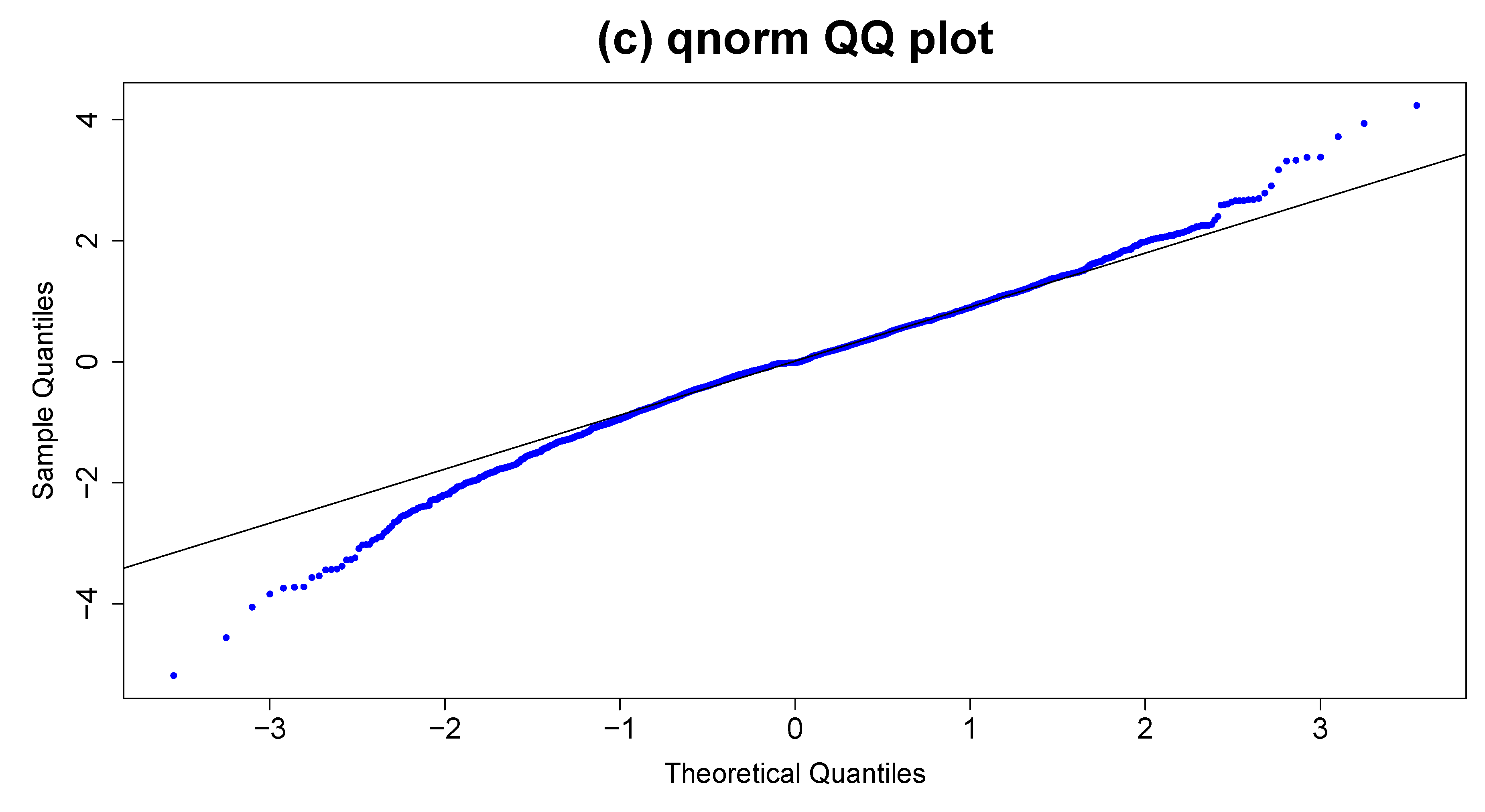
The plot of the estimated conditional standard deviations depicted in Figure 8 illustrates the presence of volatility clustering. However, when examining the time series of standardised squared residuals in Figure 7 (the second plot of the panel), it is evident that they tend to stabilise with minimal clustering. To evaluate the normality of the standardised residuals, a Q-Q plot is presented in Figure 9. This plot indicates a deviation from a straight line, suggesting that the standardised residuals do not follow a normal distribution. Additionally, the p-value obtained from the Jarque-Bera test is , which is significantly lower than 0.05, leading to the rejection of the normality assumption for the standardised residuals. The ACF of the standardised squared residuals shown in Figure 7 (the third plot of the panel) reveals no signs of autocorrelation, except at lag 13. Similar findings were also reported by the Box-Ljung test conducted above.
Figure 7.
The ACF plot for squared standardised residuals.
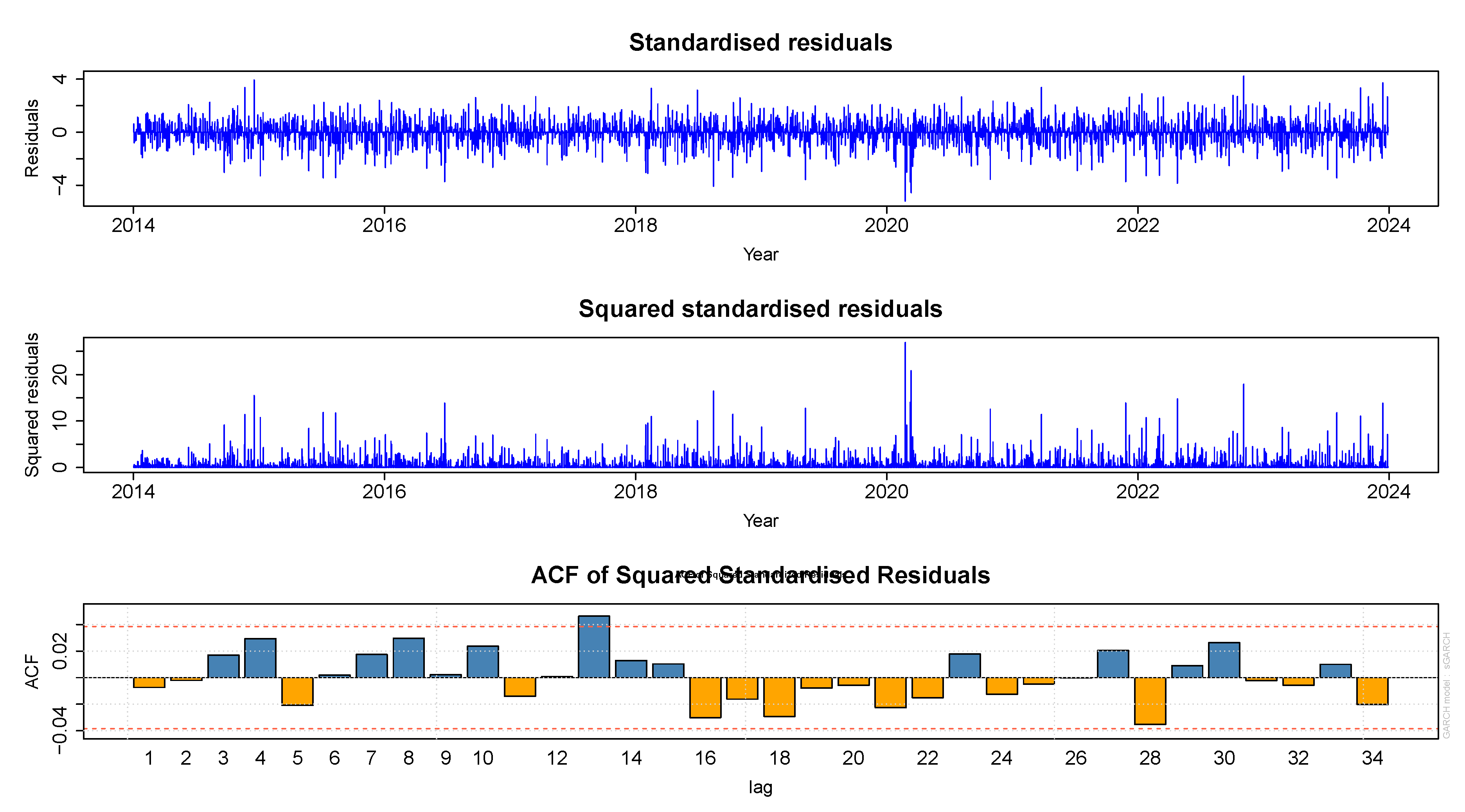
Figure 8.
The plot of estimated conditional standard deviations.
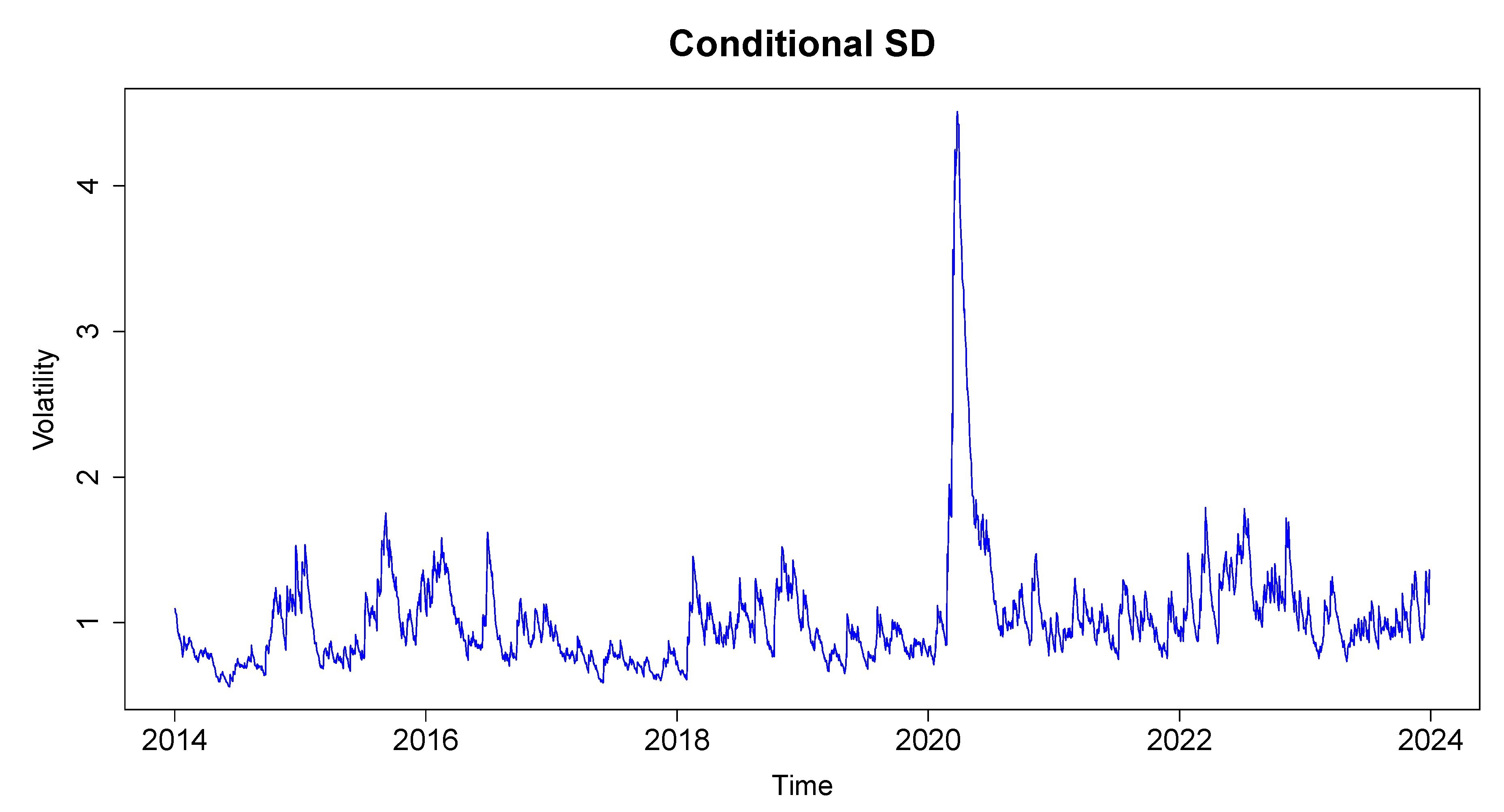
Figure 9.
Q-Q plot of standardised residuals.
3.3.2. fGARCH(1,1) Model Fitting
The student’s t-distribution, skewed student’s t-distribution, generalised error distribution, skewed generalised error distribution, and generalised hyperbolic distribution are fitted with ARMA(0,0)-fGARCH(1,1) model and Table 11 shows the information criteria obtained. Simiarly, as what we have discussed in the above subsection, Table 12 shows the ranking of different conditional distributions fitted with ARMA(0,0)- fGARCH(1,1) from the lowest to the highest value based on their respective information criteria in the Table 11. Based on the outcomes presented in Table 12, the skewed generalised error distribution seems to be a dominant conditional distribution, thus the ARMA(0,0)-fGARCH(1,1) with skewed generalised error distribution is the best fitting fGARCH model. The fGARCH model was fitted with ALLGARCH model as a submodel.
3.4. Overall Best Fitting Model
Table 13 presents the ARMA(0,0)-sGARCH(1,1) and ARMA(0,0)-fGARCH(1,1) models, both fitted using the skewed generalised error distribution, along with their respective information criteria. The results indicate that the ARMA(0,0)-fGARCH(1,1) model exhibits the lowest information criteria when compared to the ARMA(0,0)-sGARCH(1,1) model. This suggests that the ARMA(0,0)-fGARCH(1,1) model with SGED is the most suitable model for capturing the dynamics of the JSE ALSI returns’ volatility.
The other reasons why the ARMA(0,0)-fGARCH(1,1) model outperforms the ARMA(0,0)-sGARCH(1,1) model is that: the fGARCH model is more flexible in capturing asymmetries in the volatility process, such as leverage effects, where negative returns might lead to higher volatility than positive returns of the same magnitude. This flexibility allows it to better model the behavior of financial time series that exhibit such characteristics.
The fGARCH model can incorporate various forms of conditional heteroskedasticity, such as the EGARCH, ALLGARCH or TGARCH models. These can be more adept at capturing the actual volatility dynamics of the JSE ALSI, which might be influenced by factors like sudden market shifts or changes in investor sentiment and the fGARCH model often provides better out-of-sample volatility forecasts compared to the sGARCH model.
3.5. Model Diagnostics for the Qverall Best Fitting Model
Figure 10 illustrates volatility clustering in the fitted standardised residuals. Additionally, the plot of standardised squared residuals in Figure 11 demonstrates minimal volatility clustering with stable behavior. The ACF plot for standardised squared residuals, shown in Figure 12, indicates no significant autocorrelation except at lag 13. To confirm this results, the Box-Ljung test was conducted on the standardised squared residuals. As seen in Table 14, p-values at all tested lags exceed the significance threshold of 0.05, suggesting the absence of residual autocorrelation. Table 15 presents the ARCH LM test results for the ARMA(0,0)-fGARCH(1,1) model, where p-values at tested lags also exceed 0.05, indicating no remaining heteroskedasticity in the fitted model.
Table 16 displays the outcomes of the sign bias test, which assesses asymmetries in the volatility model to determine if positive and negative shocks have varying impacts on subsequent volatility. The p-values for the sign bias, negative sign bias, positive sign bias, and the joint effect all exceed 0.05, indicating a meaningful response to both positive and negative shocks. The ARMA(0,0)-fGARCH(1,1) model with SGED effectively reflects the leverage effect in the JSE ALSI returns and successfully captures volatility clustering.
The Nyblom stability test is used to assess parameter’s stability over time. A stable model should have constant parameters throughout the sample period. Table 17 shows that the parameters are stable in the model with both ARCH and GARCH effects being significant. The 1% significance level sets critical thresholds at 0.75 for individual parameters and 2.82 for the joint parameters. For this model, the joint statistic is 2.7179, which is below the critical value. Among individual parameters, the Nyblom stability test indicates that shows temporal variation, while other parameters remain stable. Table 18 lists the estimated parameters for the ARMA(0,0)-fGARCH(1,1) model with SGED, along with their respective p-values. The results in Table 18 reveal that all parameter estimates, except for the mean (with a p-value above 0.05), are statistically significant, with p-values below 0.05.
Figure 13 demonstrates that the empirical density indicates a better fit with the skewed generalised error distribution (SGED) compared to the normal density. The Q-Q plot for SGED illustrates that most data points align closely with the fitted SGED line, though some deviation appears in the tails.
3.6. Impact on Volatility
The news impact curve presented in Figure 14 illustrates that negative news has a more pronounced effect on volatility than positive news, with volatility responding more sharply to negative shocks. The estimated impact for positive shocks is , while for negative shocks, it is . The positive value of suggests that negative events influence volatility to a greater extent than positive ones. Additionally, the high persistence in the JSE ALSI returns, with a value of 0.935977, indicates a prolonged period for volatility to subside following a shock.
The plot in Figure 15 compares the time-varying conditional variance (blue line) with the long-run unconditional variance (red dashed line) for the JSE ALSI. The conditional variance fluctuates significantly over time, indicating that market volatility is not constant but rather dynamic, responding to recent events. Notably, there are clear spikes in the conditional variance, with the most prominent peak occurring around 2020, likely corresponding to a significant market event (possibly the COVID-19 pandemic), which caused a sharp increase in volatility. This suggests that during periods of bad news, volatility rises sharply, reflecting the heightened uncertainty and risk in the market.
In contrast, the unconditional variance, represented by the red dashed line, remains relatively flat. This variance is constant and represents the long-term average level of volatility expected in the market. Considering that the unconditional variance is much lower than the conditional variance during the 2020 spike indicates that the market’s reaction to the shock was temporary, with volatility eventually expected to return to more normal levels.
Throughout the sample period, the conditional variance exhibits volatility clustering, where periods of high volatility tend to follow one another, as seen between 2016 and 2021. These fluctuations suggest that risk in the JSE ALSI varies significantly depending on market conditions, but over the long run, the market tends to revert toward the lower unconditional variance.
Overall, the plot demonstrates that while short-term volatility (conditional variance) can deviate significantly due to market shocks, the long-run volatility (unconditional variance) remains stable, suggesting that the market eventually returns to its historical volatility levels once the effects of shocks dissipate.
3.7. Forecasting with the ARMA(0,0)-fGARCH(1,1) Model
Table 19 displays the predicted volatilities for the following 10 days based on the selected model. Figure 16 shows forecasts increase in volatility of the JSE ALSI over the next ten days based on the sample selected. The rate of increase varies with market fluctuations, highlighting the role of forecast updates in accounting for these changes.
4. Conclusion
This study examined the volatility of JSE ALSI returns, which exhibited leptokurtic characteristics and a slight leftward skew, using sGARCH(1,1) and fGARCH(1,1) models under five error distribution assumptions. The optimal mean model, identified as ARMA(0,0) using the auto.arima() function, was fitted with these volatility models. The ARMA(0,0)-fGARCH(1,1) model with skewed generalised error distribution provided the best fit based on information criteria. Key findings revealed high persistence in volatility, indicating that shocks to the market have a prolonged impact, with volatility decaying slowly over time. Additionally, significant autocorrelation, heteroscedasticity, and a leverage effect were observed, where negative shocks amplified volatility more than positive shocks. The Covid-19 pandemic had a pronounced impact on volatility, highlighting the market’s sensitivity to external shocks. Limitations included model assumptions and sensitivity to specification and outliers, which may affect prediction reliability. Future research could address these gaps by employing advanced methods such as artificial neural networks, GAS models, or multivariate GARCH frameworks to explore time-varying dynamics and sectoral interdependencies.
Author Contributions
Conceptualization, I.M., T.R. and C.S.; methodology, I.M.; software, I.M.; validation, I.M., T.R. and C.S.; formal analysis, I.M.; investigation, I.M., T.R. and C.S.; data curation, I.M.; writing—original draft preparation, I.M.; writing—review and editing, I.M., T.R. and C.S.; visualisation, I.M.; supervision, T.R. and C.S.; project administration, T.R. and C.S.; funding acquisition, I.M. All authors have read and agreed to the published version of the manuscript.
Institutional Review Board Statement
Not applicable.
Informed Consent Statement
Not applicable.
Data Availability Statement
The data were obtained from the Wall Street Journal Markets website https://www.wsj.com/market-data/quotes/index/ZA/XJSE/ALSH/historical-prices.
Acknowledgments
The support of the 2024 NRF Honours Postgraduate Scholarship towards this research is hereby acknowledged. Opinions expressed, and conclusions arrived at are those of the authors and are not necessarily to be attributed to the NRF. In addition, the authors thank the anonymous reviewers for their helpful comments on this paper.
Conflicts of Interest
The authors declare no conflicts of interest. The funders had no role in the study’s design, in the collection, analyses, or interpretation of data, in the writing of the manuscript, or in the decision to publish the results.
References
- Korkpoe, C. H., and Junior, P. O. (2018). Behaviour of Johannesburg Stock Exchange All Share Index returns: An asymmetric GARCH and news impact effects approach. SPOUDAI Journal of Economics and Business, 68(1), 26–42, Available at: http://spoudai.unipi.gr.
- Black, F. (1976). Studies of stock market volatility changes. Proceedings of the American Statistical Association, Business & Economic Statistics Section, 1976, Available at: https://cir.nii.ac.jp/crid/1570009749981528192.
- Engle, R. F. (1982). Autoregressive conditional heteroscedasticity with estimates of the variance of United Kingdom inflation. Econometrica: Journal of the Econometric Society, 50(4), 987–1007, Available at: https://www.jstor.org/stable/1912773.
- Bollerslev, T. (1986). Generalized autoregressive conditional heteroskedasticity. Journal of Econometrics, 31(3), 307–327. [CrossRef]
- Liu, H.-C., and Hung, J.-C. (2010). Forecasting S&P-100 stock index volatility: The role of volatility asymmetry and distributional assumption in GARCH models. Expert Systems with Applications, 37(7), 4928–4934. [CrossRef]
- Sariannidis, N., Konteos, G., and Drimbetas, E. (2009). Volatility linkages among India, Hong Kong, and Singapore stock markets. International Research Journal of Finance and Economics, 58, 141–149, Available at: https://ssrn.com/abstract=1340591.
- Horng, W., Hu, T.-C., Tsai, J., et al. (2009). Dynamic relatedness analysis of two stock market returns volatility: An empirical study on the South Korean and Japanese stock markets. Asian Journal of Management and Humanity Sciences, 4(1), 1–15, Available at: https://www.researchgate.net/profile/Tien-Chung-Hu/publication/237562195.
- Sigauke, C. (2016). Volatility modeling of the JSE all share index and risk estimation using the Bayesian and frequentist approaches. Economics, Management, and Financial Markets, 11(4), 33–48, Available at: https://www.ceeol.com/search/article-detail?id=471925.
- Engle, R. F., and Bollerslev, T. (1986). Modelling the persistence of conditional variances. Econometric Reviews, 5(1), 1–50. [CrossRef]
- Glosten, L. R., Jagannathan, R., and Runkle, D. E. (1993). On the relation between the expected value and the volatility of the nominal excess return on stocks. The Journal of Finance, 48(5), 1779–1801. [CrossRef]
- Ding, Z., Granger, C. W. J., and Engle, R. F. (1993). A long memory property of stock market returns and a new model. Journal of Empirical Finance, 1(1), 83–106. [CrossRef]
- Nelson, D. B. (1991). Conditional heteroskedasticity in asset returns: A new approach. Econometrica: Journal of the Econometric Society, 59(2), 347–370. [CrossRef]
- Hentschel, L. (1995). All in the family nesting symmetric and asymmetric GARCH models. Journal of Financial Economics, 39(1), 71–104. [CrossRef]
- Mandelbrot, B. B. (1997). The variation of certain speculative prices. Springer, Available at: https://www.jstor.org/sici?sici=0021-9398%28196310%2936%3A4%3C394%3ATVOCSP%3E2.0.CO%3B2-L.
- Fama, E. F. (1965). The behavior of stock-market prices. The Journal of Business, 38(1), 34–105, Available at: https://www.jstor.org/stable/2350752.
- Christie, A. A. (1982). The stochastic behavior of common stock variances: Value, leverage and interest rate effects. Journal of Financial Economics, 10(4), 407–432. [CrossRef]
- Bollerslev, T., Chou, R. Y., and Kroner, K. F. (1992). ARCH modeling in finance: A review of the theory and empirical evidence. Journal of Econometrics, 52(1-2), 5–59. [CrossRef]
- Aron, J., Elbadawi, I., et al. (1999). Reflections on the South African rand crisis of 1996 and policy consequences. Tech Report, Available at: https://ideas.repec.org/p/csa/wpaper/1999-13.html.
- Olweny, T., and Omondi, K. (2011). The effect of macro-economic factors on stock return volatility in the Nairobi stock exchange, Kenya. Economics and Finance Review, 1(10), 34–48, Available at: http://www.businessjournalz.org/efr.
- Olowe, R. A. (2009). Modelling naira/dollar exchange rate volatility: Application of GARCH and asymmetric models. International Review of Business Research Papers, 5(3), 377–398, Available at: https://scholar.google.com/scholar?hl=en&as_sdt=0%2C5&q=%5Cbibitem%7Bolowe2009modelling%7D+Olowe%2C+R.+A.+%282009%29.++Modelling+naira%2Fdollar+exchange+rate+volatility%3A+Application+of+GARCH+and+asymmetric+models.++%5Ctextit%7BInternational+Review+of+Business+Research+Papers%7D%2C+5%283%29%2C+377–398.&btnG=.
- Onwukwe, C. E., Bassey, B. E. E., and Isaac, I. O. (2011). On modeling the volatility of Nigerian stock returns using GARCH models. Journal of Mathematics Research, 3(4), 31, Available at: https://www.researchgate.net/publication/265772472_On_Modeling_the_Volatility_of_Nigerian_Stock_Returns_Using_GARCH_Models.
- Cifter, A. (2012). Volatility forecasting with asymmetric normal mixture GARCH model: Evidence from South Africa. Inst Economic Forecasting, Available at: https://www.researchgate.net/profile/AtillaCifter/publication/254449039_Volatility_Forecasting_with_Asymmetric_Normal_Mixture_Garch_Model_Evidence_from_South_Africa/links/54761e7b0cf2778985b07ada.
- Makhwiting, M. R. (2014). Modelling volatility and financial market risks of shares on the Johannesburg stock exchange. MSc Thesis, Available at: http://hdl.handle.net/10386/1389.
- Mzamane, T. P. (2013). GARCH modelling of volatility in the Johannesburg Stock Exchange index. PhD Thesis, Available at: https://researchspace.ukzn.ac.za.
- Niyitegeka, O., and Tewar, D. D. (2013). Volatility clustering at the Johannesburg Stock Exchange: Investigation and analysis. Mediterranean Journal of Social Sciences, 4(14), 621–626.
- Harvey, A., and Sucarrat, G. (2014). EGARCH models with fat tails, skewness and leverage. Computational Statistics & Data Analysis, 76, 320–338. [CrossRef]
- Xia, Q., Liang, R., and Liu, J. (2015). A Bayesian analysis of autoregressive models with exogenous variables and power-transformed and threshold GARCH errors. Communications in Statistics-Theory and Methods, 44(9), 1967–1980, Available at: https://www.tandfonline.com/doi/full/10.1080/03610926.2013.863926. [CrossRef]
- Brailsford, T. J., and Faff, R. W. (1996). An evaluation of volatility forecasting techniques. Journal of Banking & Finance, 20(3), 419–438. [CrossRef]
- Engle, R. F., and Ng, V. K. (1993). Measuring and testing the impact of news on volatility. The Journal of Finance, 48(5), 1749–1778. [CrossRef]
- Angabini, A., and Wasiuzzaman, S. (2011). GARCH models and the financial crisis: A study of the Malaysian. The International Journal of Applied Economics and Finance, 5(3), 226–236, Available at: https://scialert.net/abstract/?doi=ijaef.2011.226.236.
- Junior, T. P., Lima, F. G., and Gaio, L. E. (2014). Volatility behaviour of BRIC capital markets in the 2008 international financial crisis. African Journal of Business Management, 8(11), 1, Available at: https://academicjournals.org/journal/AJBM/article-full-text-pdf/ADB029645072.
- Rusere, W., and Kaseke, F. (2021). Modeling South African stock market volatility using univariate symmetric and asymmetric GARCH models. Indian Journal of Finance and Banking, 6(1), 1–16. [CrossRef]
- Engle, R. (2004). Risk and volatility: Econometric models and financial practice. American Economic Review, 94(3), 405–420, Available at: https://www.aeaweb.org/articles?id=10.1257/0002828041464597.
- Brooks, C. (2008). RATS Handbook to accompany introductory econometrics for finance. Cambridge Books, Cambridge University Press, Available at: https://ideas.repec.org/b/cup/cbooks/9780521721684.html.
- Ghalanos, A. (2019). rmgarch: Multivariate GARCH models. R Package Version 1.4-0, Available at: https://cran.r-project.org/package=rmgarch.
Figure 1.
JSE ALSI closing stock prices.
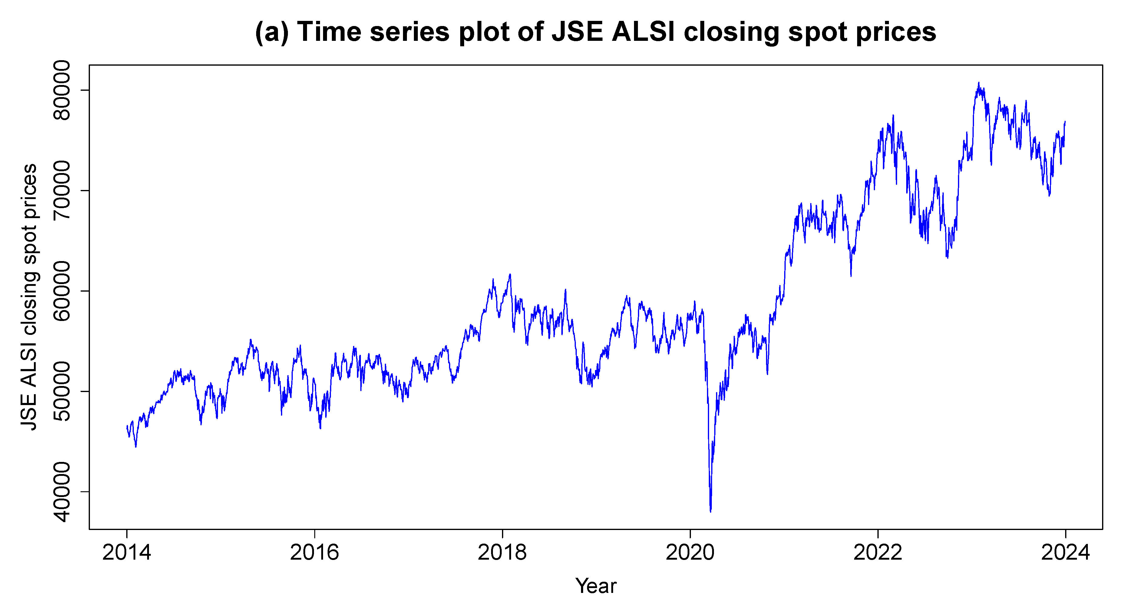
Figure 2.
Decomposition of time series for the log returns of the JSE ALSI.
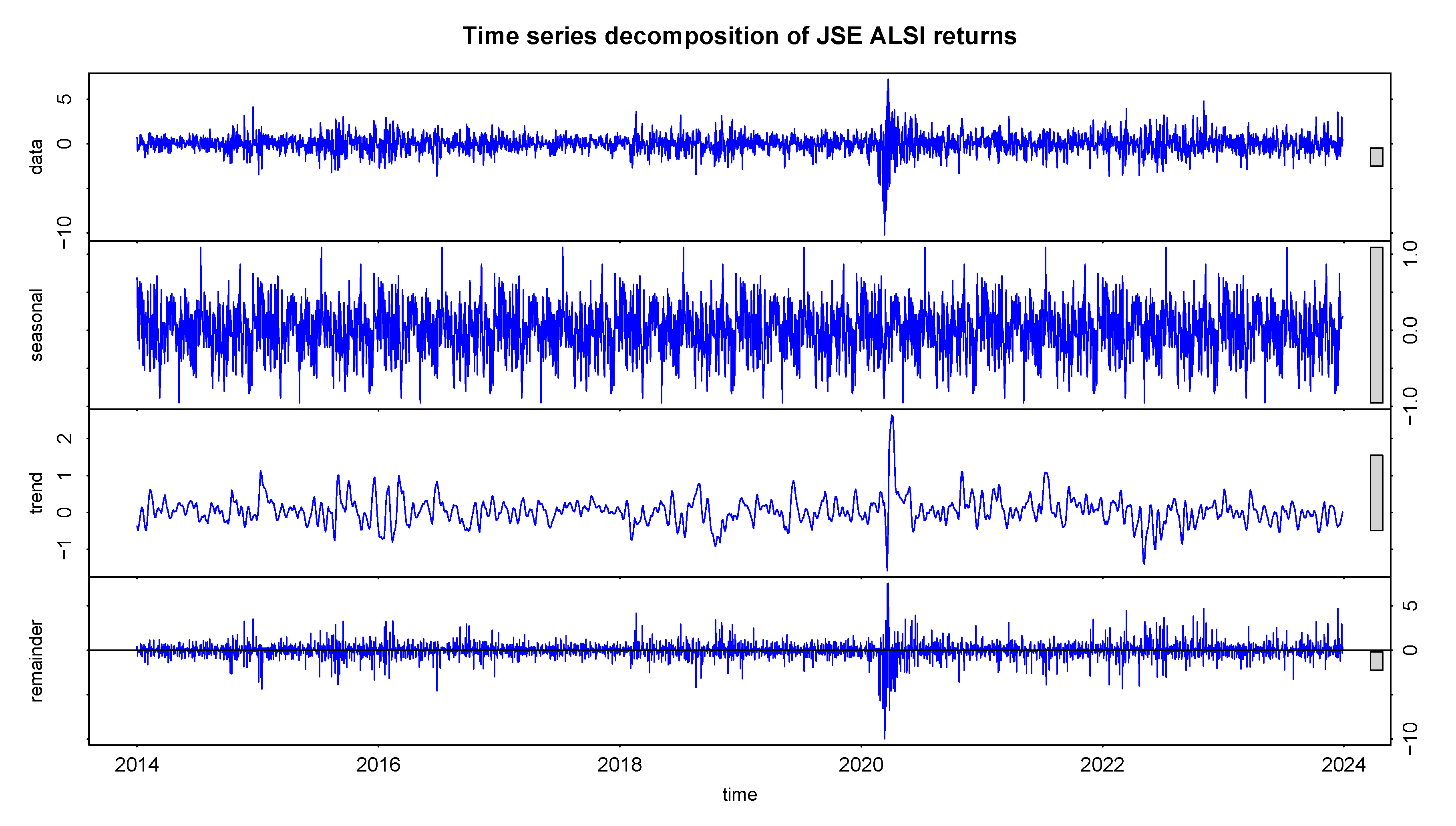
Figure 3.
The trend component of return series.
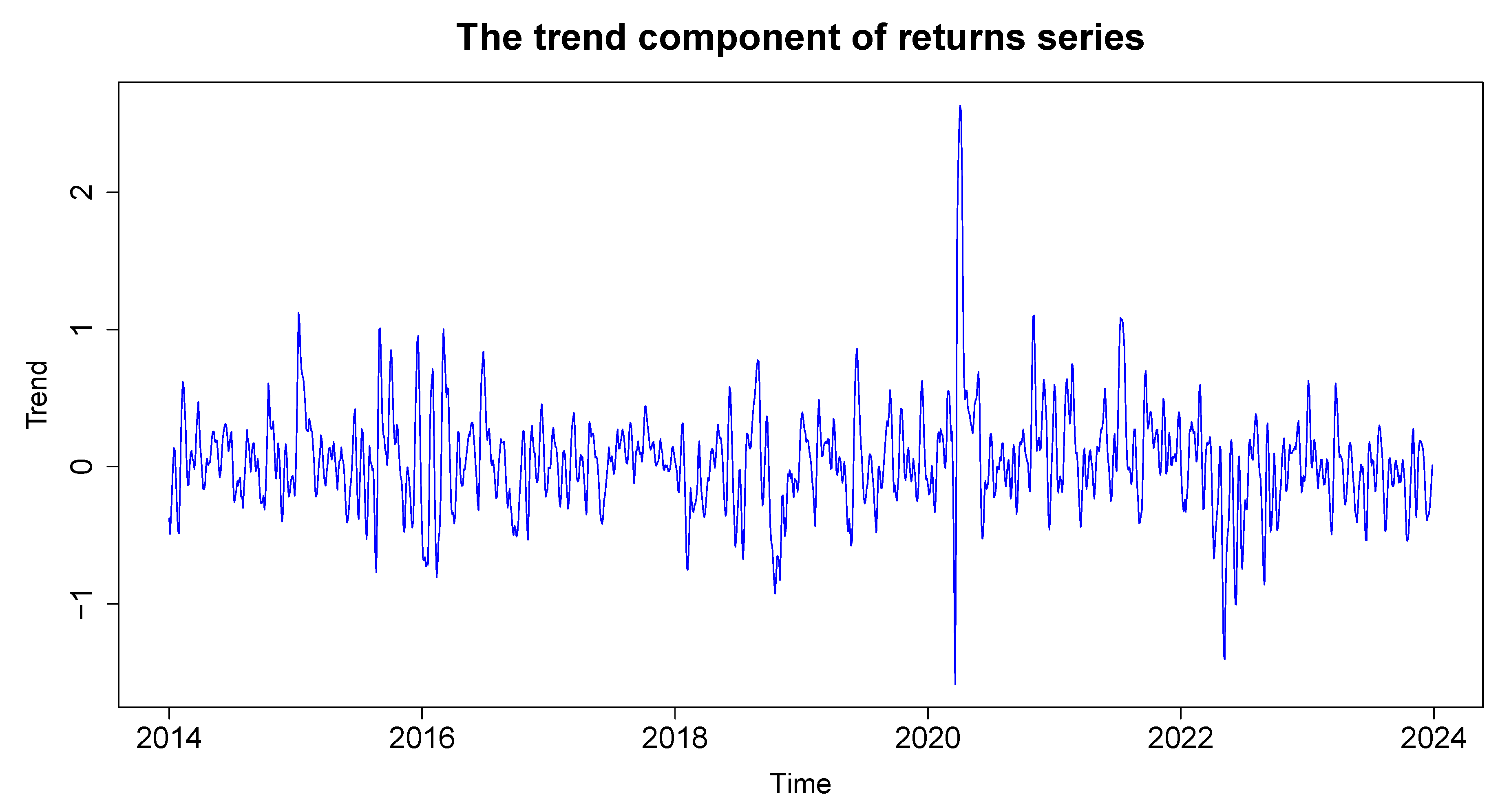
Figure 4.
(a) JSE All-Share Index plot (top left panel), (b) Daily log-returns for JSE Stock Index (top right panel), (c) Density plot of daily log-returns (bottom left panel), and (d) Normal Q-Q Plot of daily log-returns (bottom right panel).
Figure 4.
(a) JSE All-Share Index plot (top left panel), (b) Daily log-returns for JSE Stock Index (top right panel), (c) Density plot of daily log-returns (bottom left panel), and (d) Normal Q-Q Plot of daily log-returns (bottom right panel).
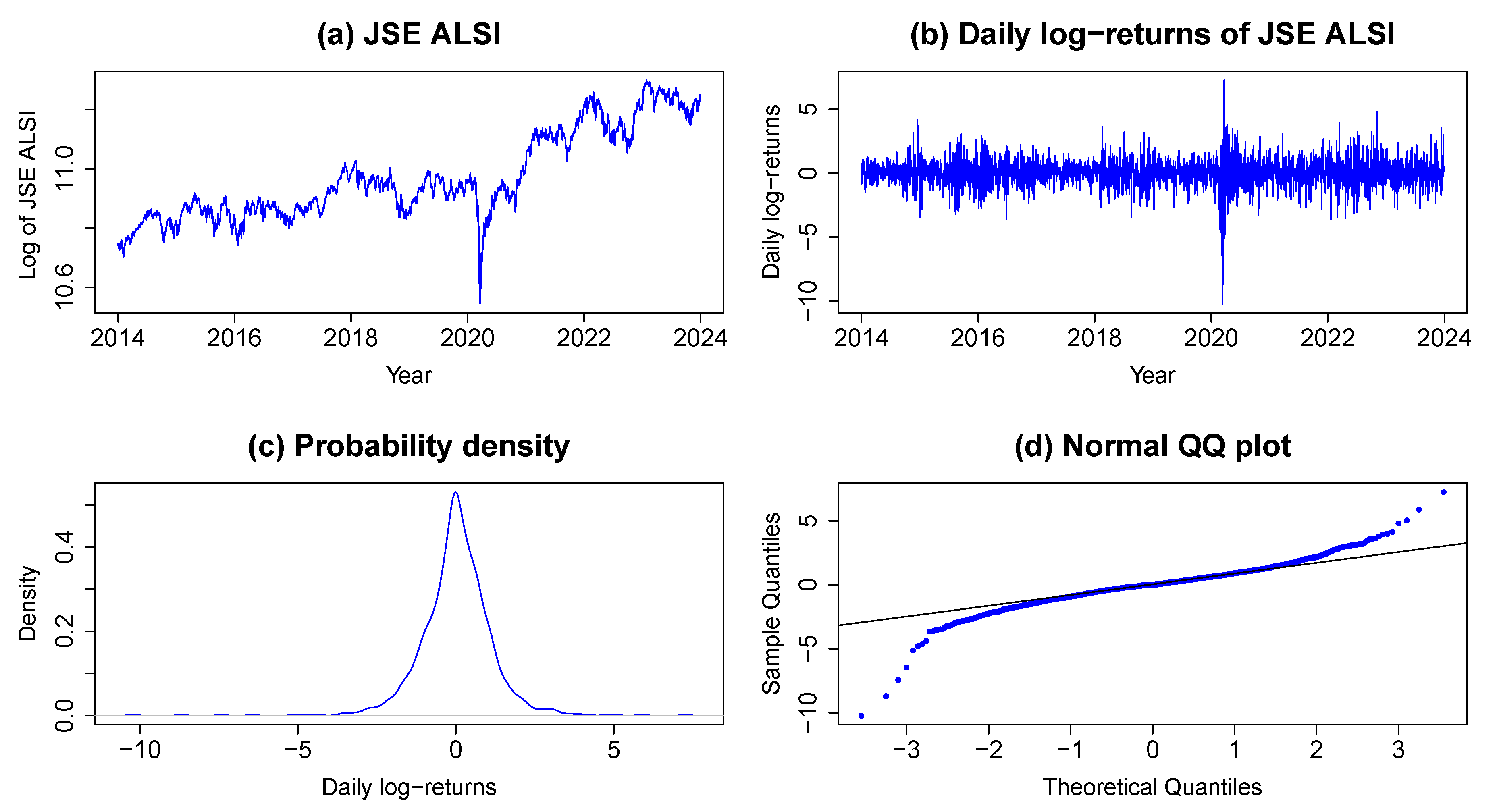
Figure 5.
ACF and PACF for JSE ALSI return series.
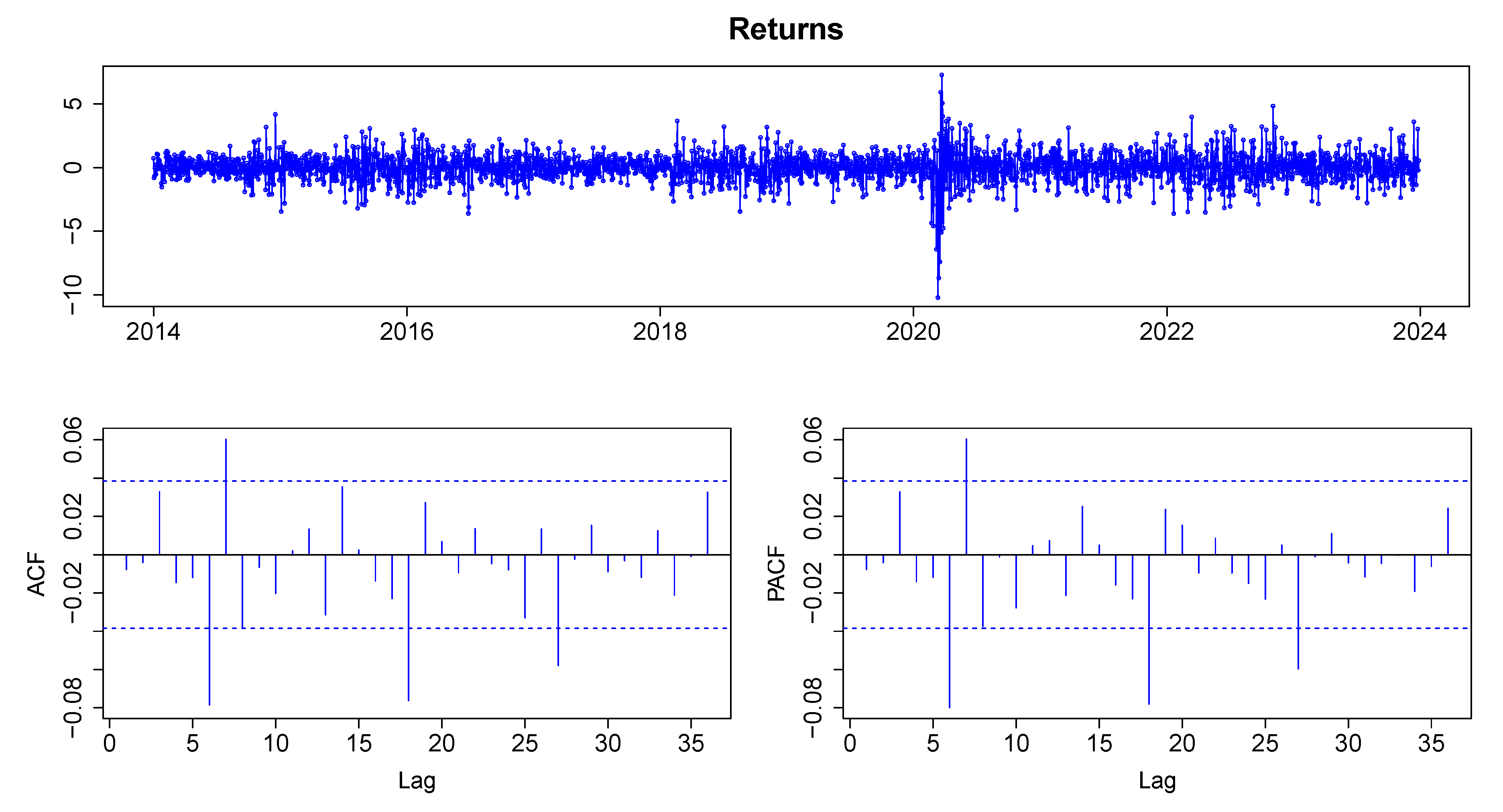
Figure 6.
ACF and PACF of squared JSE ALSI returns.
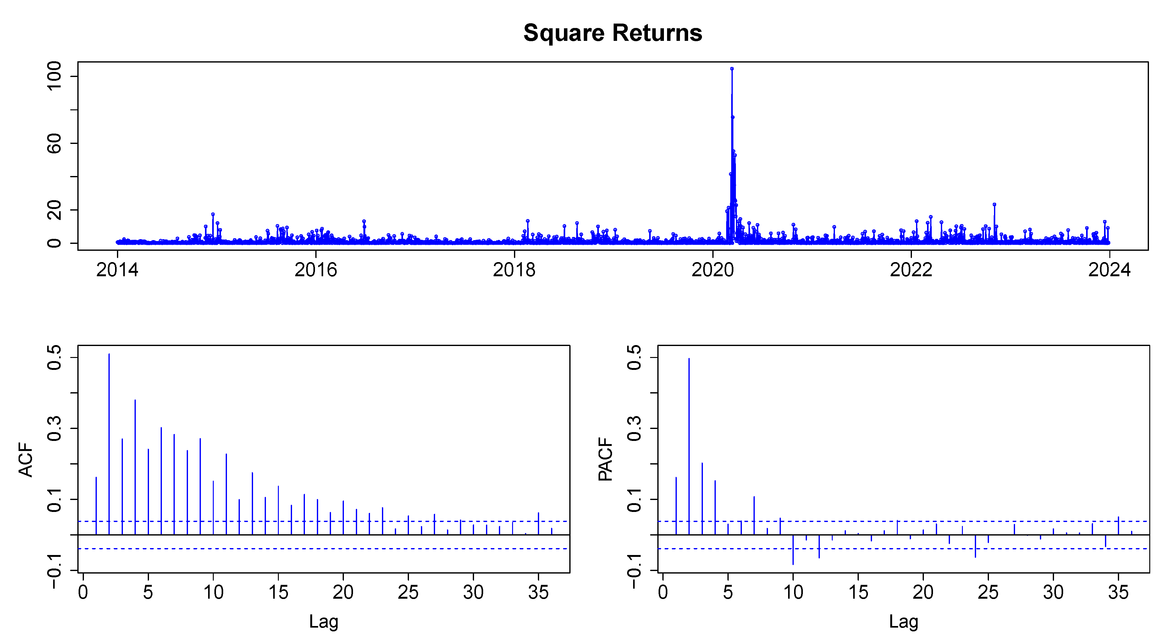
Figure 10.
Comparison of residuals and estimated conditional standard deviations.
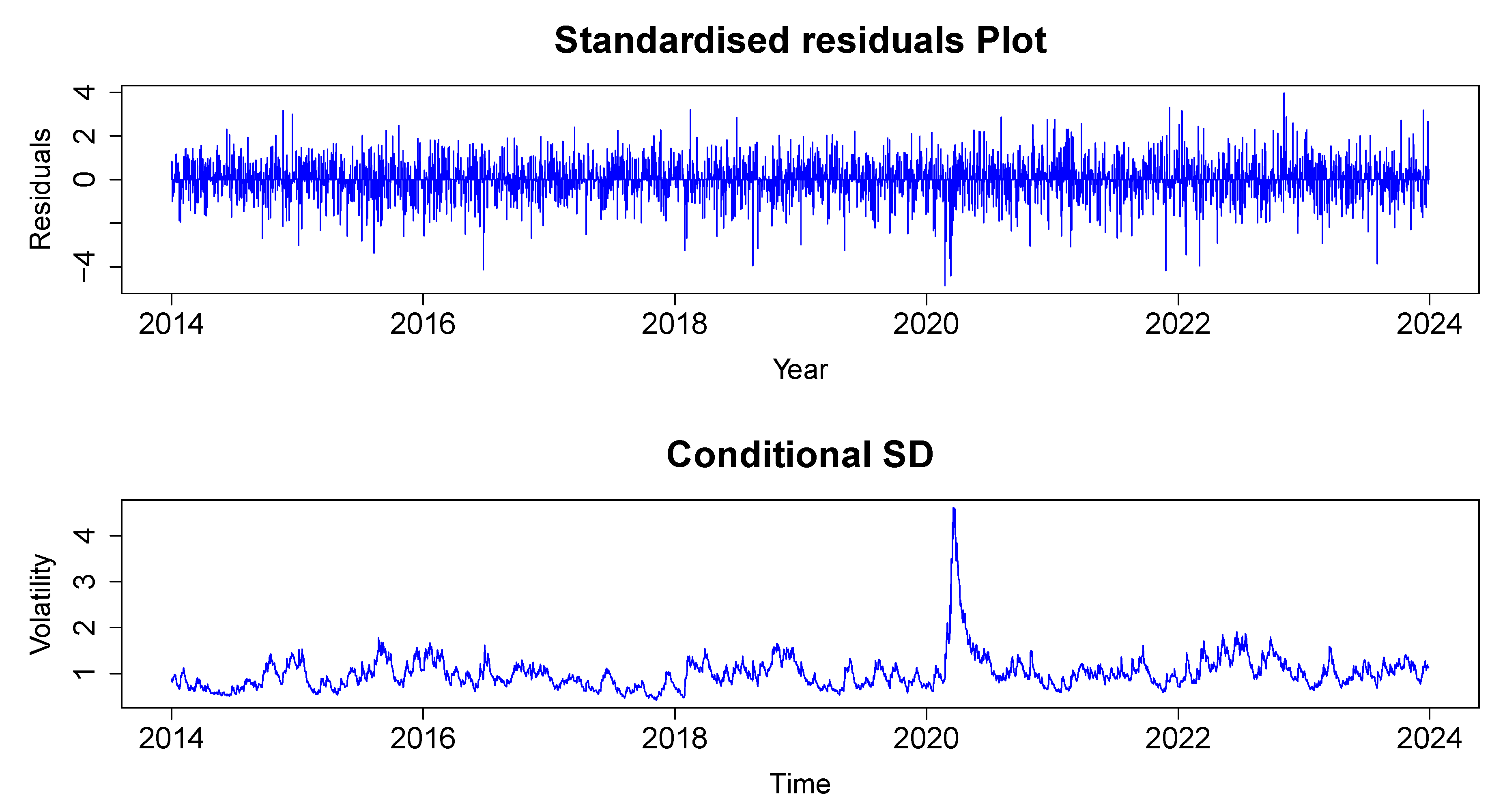
Figure 11.
Standardised squared residuals of ARMA(0,0)-fGARCH(1,1).
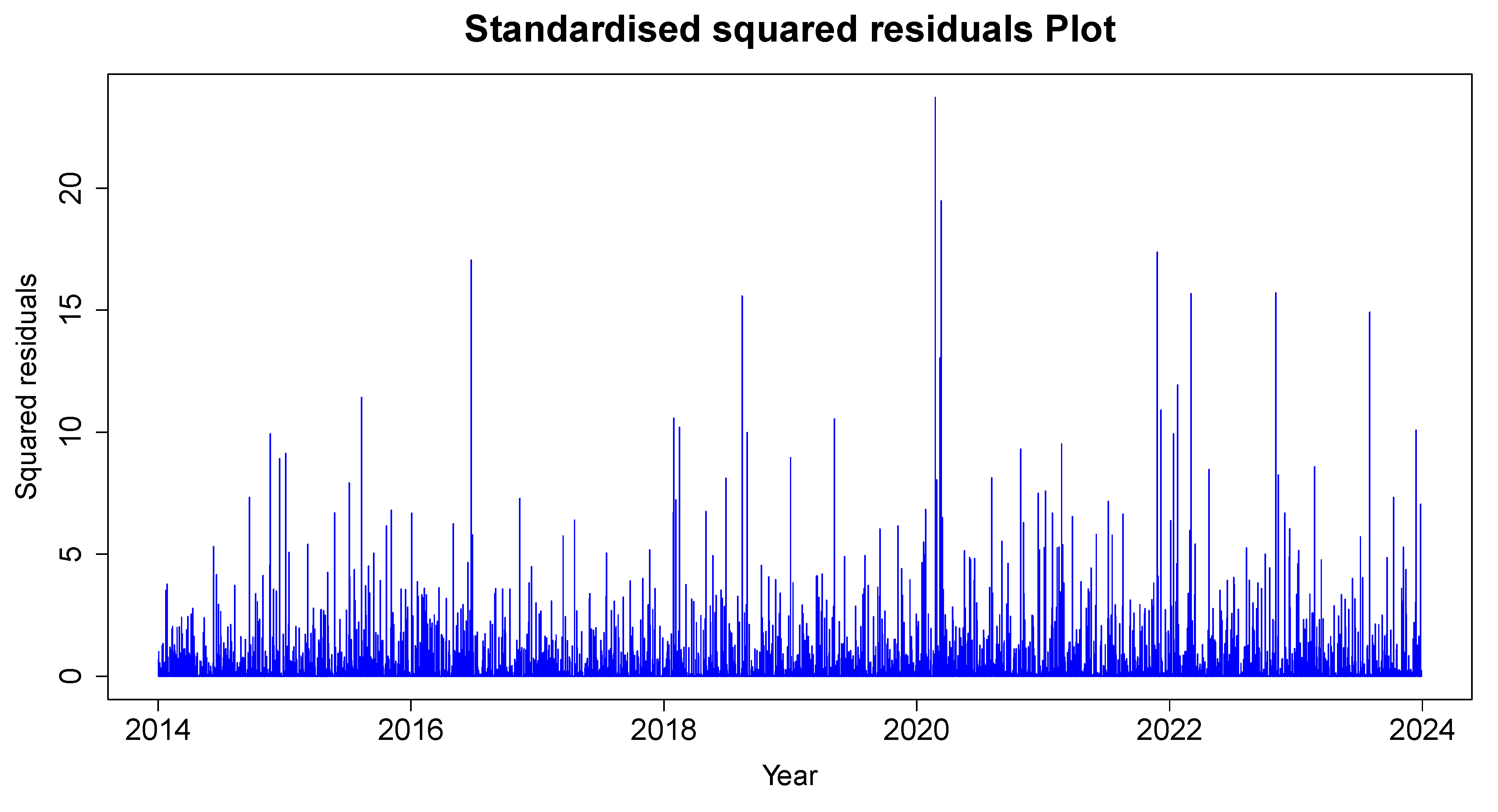
Figure 12.
ACF plot for the squared standardised residuals.
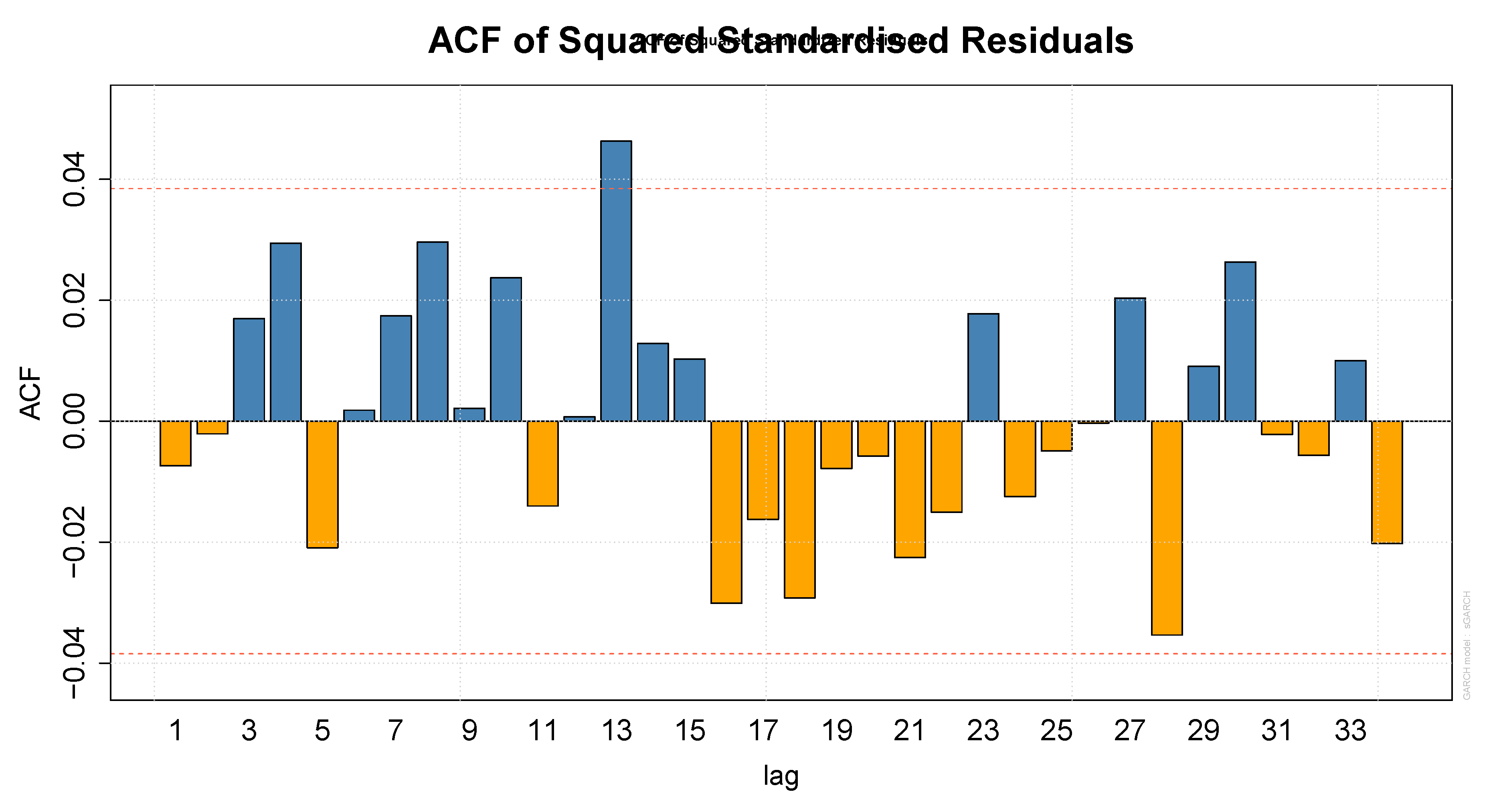
Figure 13.
Q-Q and Empirical Density plots of the standardised residuals.
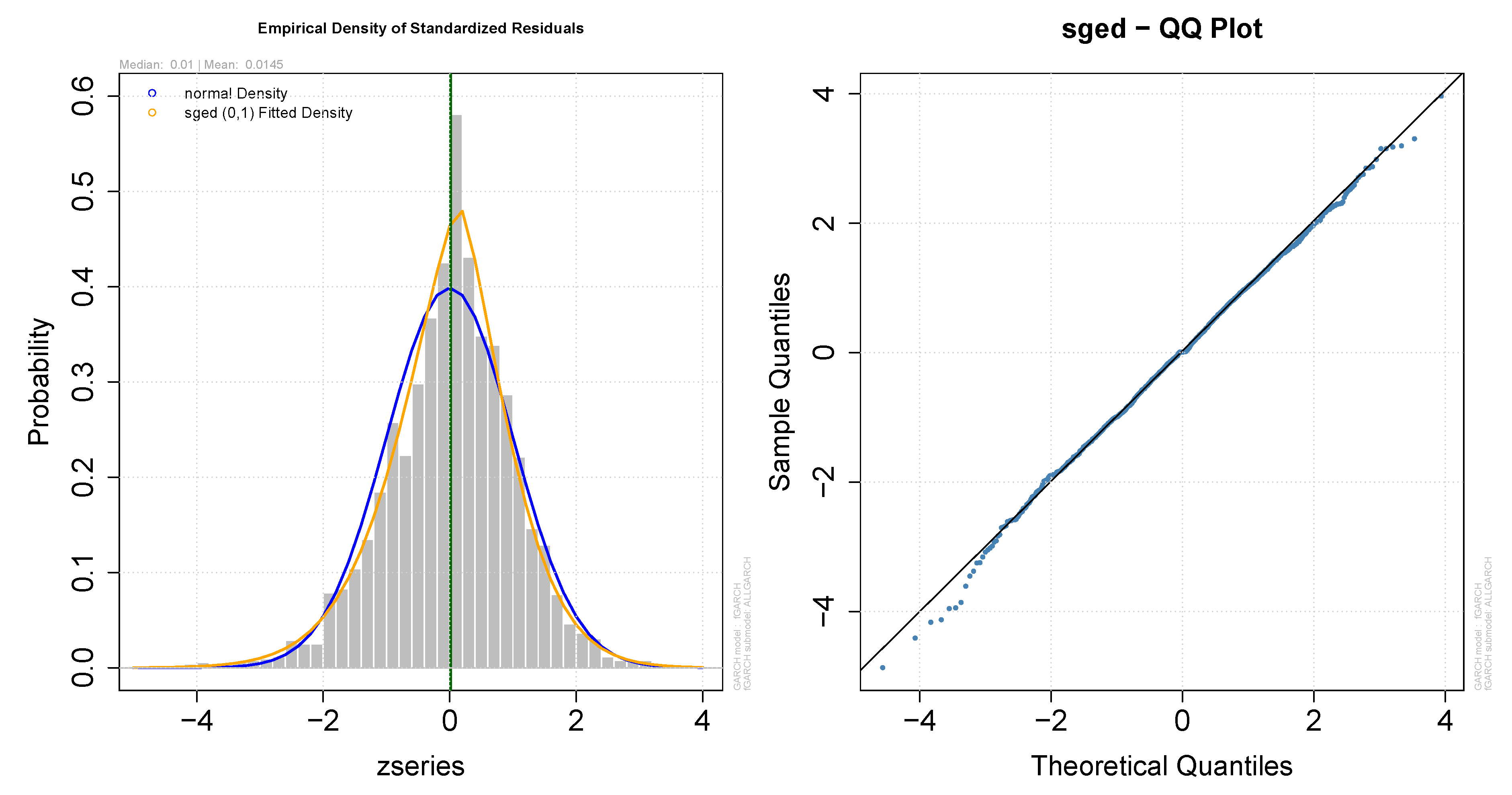
Figure 14.
Impact curve.
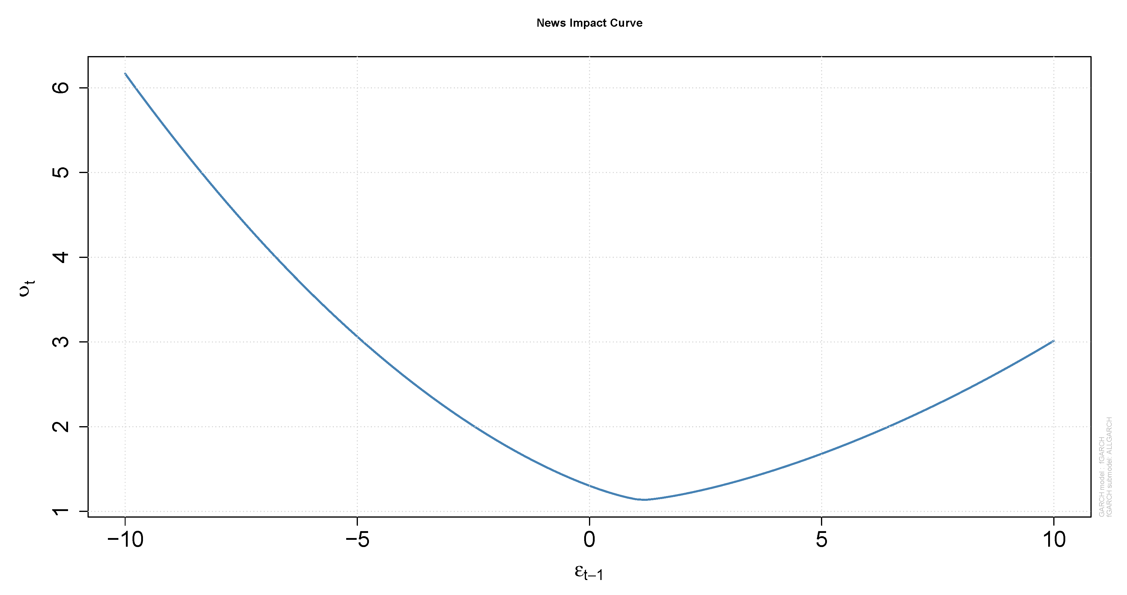
Figure 15.
Condition and Unconditional variance.
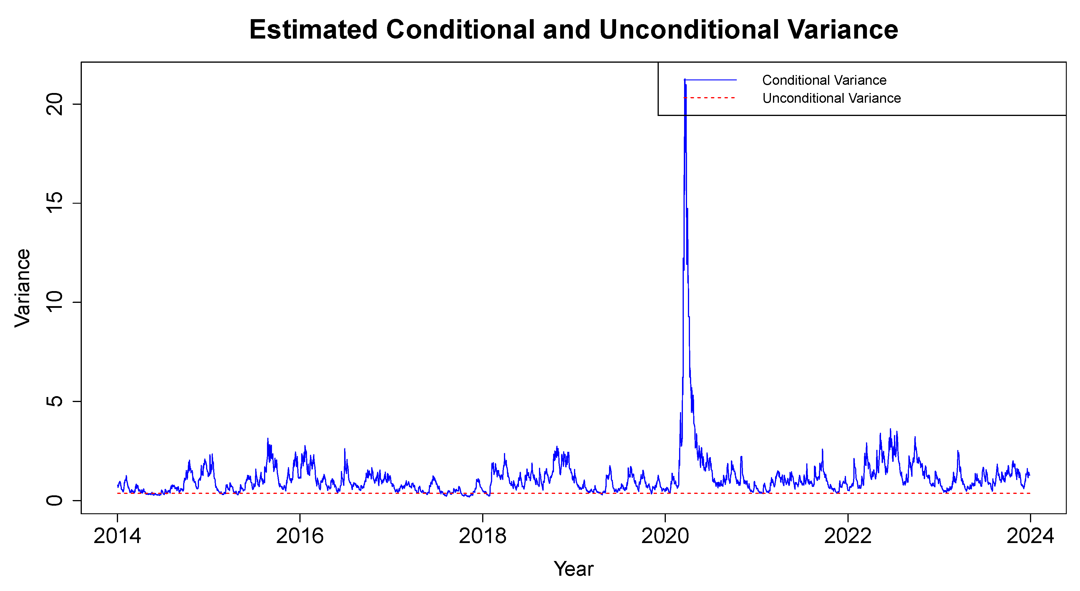
Figure 16.
Plot of the forecasted volatility over the following ten days.
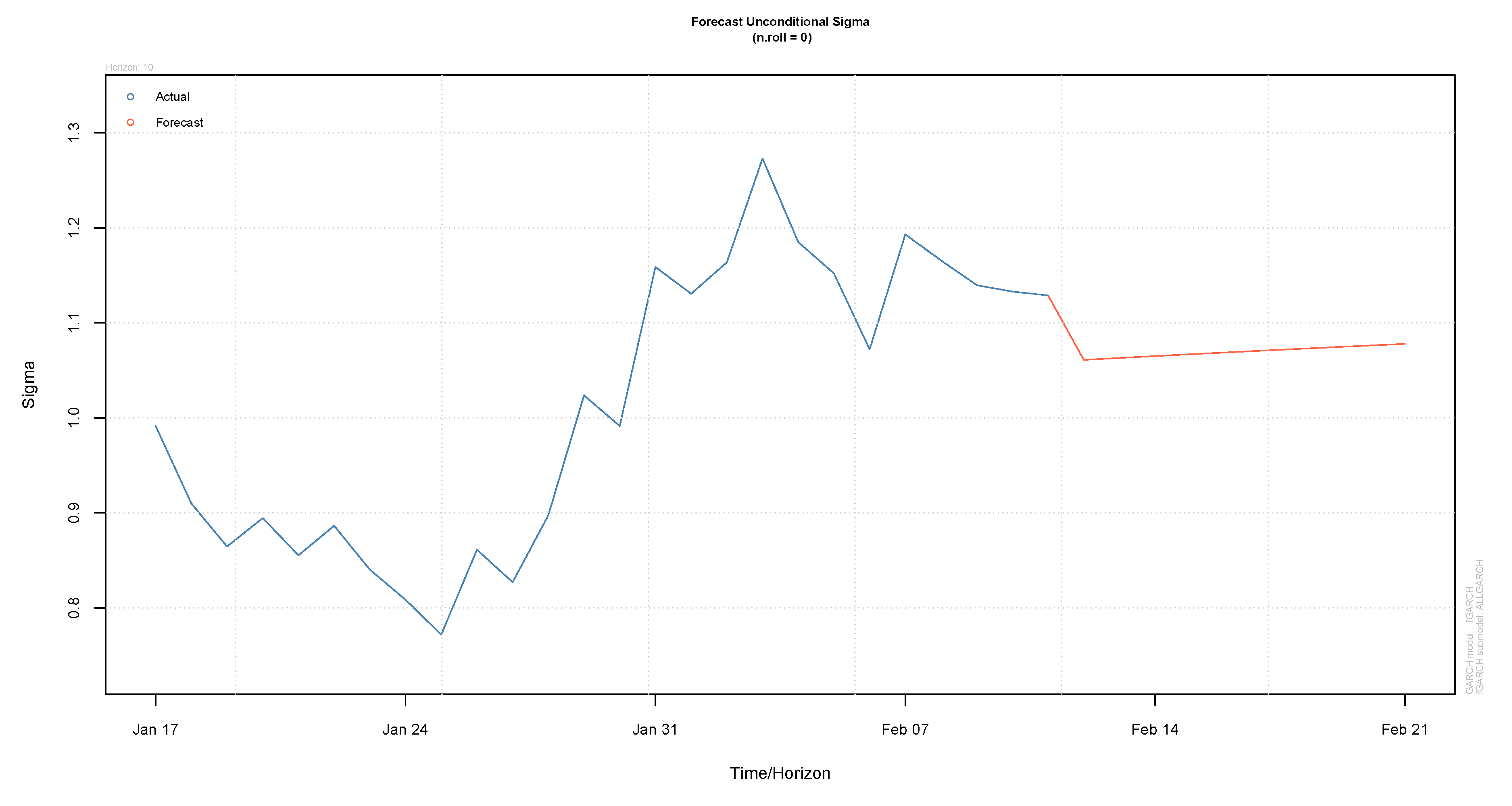

Table 1.
Results of normality and stationarity tests for returns.
| Test | Results |
|---|---|
| KPSS | Test Statistic: 0.022348 |
| p-value: 0.1 | |
| Decision: Stationary | |
| ADF | Test Statistic: -13.955 |
| p-value: 0.01 | |
| Decision: Stationary | |
| Jarque-Bera | Test Statistic: 6565 |
| p-value: | |
| Decision: Non-Normal |
Table 2.
Descriptive statistics of the JSE ALSI closing stock prices.
| Statistic | Estimate |
|---|---|
| Minimum | 37963 |
| Maximum | 80791 |
| 1st Quartile | 51912 |
| Median | 55840 |
| Mean | 58725 |
| 3rd Quartile | 66351 |
| Std. Deviation | 9086.296 |
| Kurtosis | -0.5821364 |
| Skewness | 0.7663588 |
| n | 2599 |
Table 3.
Descriptive statistics of return series.
| Statistic | Estimate |
|---|---|
| Minimum | -10.22682 |
| Maximum | 7.26147 |
| 1st Quartile | -0.51940 |
| Median | 0.00000 |
| Mean | 0.01956 |
| 3rd Quartile | 0.61427 |
| Std. Deviation | 1.096424 |
| Kurtosis | 7.699379 |
| Skewness | -0.5563153 |
| n | 2599 |
Table 4.
Summary of Box-Ljung Q test for detecting Autocorrelation.
| Lag | Results |
|---|---|
| 10 | critical value: 18.30704 |
| statistic: 34.347 | |
| p-value: 0.0001613 | |
| 15 | critical value: 24.99579 |
| statistic: 40.713 | |
| p-value: 0.0003537 | |
| 20 | critical value: 31.41043 |
| statistic: 59.853 | |
| p-value: 7.505 | |
| 36 | critical Value: 50.99846 |
| statistic: 78.612 | |
| p-value: 5.22 |
Table 5.
Summary of Engle’s ARCH LM test for detecting Heteroscedasticity.
| Lag | Results |
|---|---|
| 10 | critical value: 18.30704 |
| statistic: 778.48 | |
| p-value: | |
| 15 | critical value: 24.99579 |
| statistic: 785.77 | |
| p-value: | |
| 20 | critical value: 31.41043 |
| statistic: 792.26 | |
| p-value: | |
| 36 | critical value: 50.99846 |
| statistic: 789.05 | |
| p-value: |
Table 6.
Information criteria for ARMA(0,0)-sGARCH(1,1) with various error distributions.
| Information | M1 | M2 | M3 | M4 | M5 |
|---|---|---|---|---|---|
| criteria | |||||
| AIC | 2.7682 | 2.7651 | 2.7639 | 2.7626 | 2.7633 |
| BIC | 2.7795 | 2.7787 | 2.7752 | 2.7761 | 2.7791 |
| Hannan-Quinn | 2.7723 | 2.7700 | 2.7680 | 2.7675 | 2.7690 |
Table 7.
Ranking of different conditional distributions fitted with ARMA(0,0)-sGARCH(1,1) from the lowest to the highest value based on their respective information criteria.
Table 7.
Ranking of different conditional distributions fitted with ARMA(0,0)-sGARCH(1,1) from the lowest to the highest value based on their respective information criteria.
| No. | AIC | BIC | Hannan-Quinn |
|---|---|---|---|
| 1 | M4 | M3 | M4 |
| 2 | M5 | M4 | M3 |
| 3 | M3 | M2 | M5 |
| 4 | M2 | M5 | M2 |
| 5 | M1 | M1 | M1 |
Table 8.
Estimates of parameters for the ARMA(0,0)-sGARCH(1,1) model.
| Parameter | Estimate | Std.Error | t-value | p-value |
|---|---|---|---|---|
| 0.023106 | 0.017586 | 1.3139 | 0.188869 | |
| 0.022579 | 0.008160 | 2.7670 | 0.005657 | |
| 0.077131 | 0.013233 | 5.8286 | 0.000000 | |
| 0.903484 | 0.017303 | 52.2147 | 0.000000 | |
| skew | 0.937336 | 0.022573 | 41.5242 | 0.000000 |
| shape | 1.367764 | 0.053756 | 25.4440 | 0.000000 |
Table 9.
Results of the Weighted Ljung-Box test on standardised squared residuals.
| Lag | Statistic | p-value |
|---|---|---|
| 1 | 0.1414 | 0.7069 |
| 5 | 1.7295 | 0.6836 |
| 9 | 3.6470 | 0.6491 |
Table 10.
Results of the Weighted ARCH LM test on standardised residuals.
| Lag | Statistic | Shape | Scale | p-value |
|---|---|---|---|---|
| 3 | 0.7468 | 0.500 | 2.000 | 0.3875 |
| 5 | 3.2288 | 1.440 | 1.667 | 0.2583 |
| 7 | 3.8298 | 2.315 | 1.543 | 0.3718 |
Table 11.
Information criteria for ARMA(0,0)-fGARCH(1,1) with various error distributions.
| Information criteria | M1 | M2 | M3 | M4 | M5 |
|---|---|---|---|---|---|
| AIC | 2.7348 | 2.7288 | 2.7321 | 2.7274 | 2.7280 |
| BIC | 2.7528 | 2.7492 | 2.7501 | 2.7477 | 2.7506 |
| Hannan-Quinn | 2.7413 | 2.7362 | 2.7386 | 2.7348 | 2.7362 |
Table 12.
Ranking of different conditional distributions fitted with ARMA(0,0)-fGARCH(1,1) from the lowest to the highest value based on their respective information criteria.
Table 12.
Ranking of different conditional distributions fitted with ARMA(0,0)-fGARCH(1,1) from the lowest to the highest value based on their respective information criteria.
| No. | AIC | BIC | Hannan-Quinn |
|---|---|---|---|
| 1 | M4 | M4 | M4 |
| 2 | M5 | M2 | M5 |
| 3 | M2 | M3 | M2 |
| 4 | M3 | M5 | M3 |
| 5 | M1 | M1 | M1 |
Table 13.
Information criteria for ARMA(0,0)-sGARCH(1,1) and ARMA(0,0)-fGARCH(1,1) models using the skewed generalized error distribution.
Table 13.
Information criteria for ARMA(0,0)-sGARCH(1,1) and ARMA(0,0)-fGARCH(1,1) models using the skewed generalized error distribution.
| Model | AIC | BIC | Hannan-Quinn |
|---|---|---|---|
| ARMA(0,0)-sGARCH(1,1) with SGED | 2.7626 | 2.7761 | 2.7675 |
| ARMA(0,0)-fGARCH(1,1) with SGED | 2.7274 | 2.7477 | 2.7348 |
Table 14.
Weighted Ljung-Box test on standardised squared residuals.
| Lag | Statistic | p-value |
|---|---|---|
| 1 | 0.00383 | 0.9507 |
| 5 | 1.28506 | 0.7925 |
| 9 | 3.16065 | 0.7322 |
Table 15.
Weighted ARCH LM test on standardised residuals.
| Lag | Statistic | Shape | Scale | p-value |
|---|---|---|---|---|
| 3 | 0.5065 | 0.500 | 2.000 | 0.4767 |
| 5 | 2.5569 | 1.440 | 1.667 | 0.3608 |
| 7 | 3.2562 | 2.315 | 1.543 | 0.4665 |
Table 16.
Results of the Sign Bias test.
| Test | Statistic | p-value |
|---|---|---|
| Sign bias | 0.5814 | 0.56101 |
| Negative sign bias | 0.2212 | 0.82498 |
| Positive sign bias | 1.8559 | 0.06358 |
| Joint effect | 3.8638 | 0.27656 |
Table 17.
Nyblom test for parameter stability.
| Parameter | Estimate |
|---|---|
| 0.4475 | |
| 0.9950 | |
| 0.5830 | |
| 0.6689 | |
| 0.5457 | |
| 0.5984 | |
| 0.6204 | |
| 0.2675 | |
| 0.2930 |
Table 18.
Estimated parameters.
| Parameter | Estimate | Std.Error | t-value | p-value |
|---|---|---|---|---|
| -0.008445 | 0.016695 | -0.50585 | 0.612960 | |
| 0.023173 | 0.0.002651 | 8.74128 | 0.000000 | |
| 0.070950 | 0.019066 | 3.72123 | 0.000198 | |
| 0.865027 | 0.000470 | 1841.50524 | 0.000000 | |
| 0.189341 | 0.082816 | 2.28629 | 0.022237 | |
| 0.976316 | 0.109650 | 8.90396 | 0.000000 | |
| 1.351223 | 0.228573 | 5.91156 | 0.000000 | |
| skew | 0.905463 | 0.022789 | 39.73301 | 0.000000 |
| shape | 1.469429 | 0.058833 | 24.97611 | 0.000000 |
Table 19.
Predicted volatility over the upcoming ten days.
| Series | Sigma | |
|---|---|---|
| -0.008445 | 1.061 | |
| -0.008445 | 1.063 | |
| -0.008445 | 1.065 | |
| -0.008445 | 1.067 | |
| -0.008445 | 1.069 | |
| -0.008445 | 1.071 | |
| -0.008445 | 1.073 | |
| -0.008445 | 1.074 | |
| -0.008445 | 1.076 | |
| -0.008445 | 1.078 |
Disclaimer/Publisher’s Note: The statements, opinions and data contained in all publications are solely those of the individual author(s) and contributor(s) and not of MDPI and/or the editor(s). MDPI and/or the editor(s) disclaim responsibility for any injury to people or property resulting from any ideas, methods, instructions or products referred to in the content. |
© 2025 by the authors. Licensee MDPI, Basel, Switzerland. This article is an open access article distributed under the terms and conditions of the Creative Commons Attribution (CC BY) license (http://creativecommons.org/licenses/by/4.0/).
Copyright: This open access article is published under a Creative Commons CC BY 4.0 license, which permit the free download, distribution, and reuse, provided that the author and preprint are cited in any reuse.


