Submitted:
11 February 2026
Posted:
12 February 2026
You are already at the latest version
Abstract
Trajectory planning algorithms are essential in human-robot collaboration (HRC), as they must generate efficient trajectories for seamless interaction. Given the risks and complexity of testing in real-world scenarios, a virtual environment was developed in Unity 3D, integrating a digital twin of the UR3 robot that delivers workpieces to a user equipped with a Meta Quest device. The RRT, RRT-Star (RRTS), and RRT-Connect (RRTC) algorithms were evaluated using ANOVA and Tukey post-hoc tests, considering the following response variables: safety, feasibility, smoothness, and computation time across three experimental scenarios characterized by (i) low, (ii) medium, and (iii) high levels of movement of the participant’s left hand. The statistical results indicate that RRTC exhibited the best performance in terms of smoothness and computation time. Based on these findings, a multicriteria decision-making analysis was conducted using the Analytic Hierarchy Process (AHP), combining quantitative evidence derived from the statistical analysis with expert judgments supported by bibliographic references. This multicriteria analysis enabled the coherent integration of the different evaluation criteria and concluded that RRTC is the most suitable alternative for collaborative assembly tasks in CHR environments.
Keywords:
trajectory planning algorithms
; virtual reality
; Unity 3D
; collaborative manufacturing
; open motion planning library
1. Introduction
In the manufacturing industry, human-robot interaction (HRI) has transformed the way manufacturing systems operate and adapt to the evolving demands of the market [1,2]. In this context, reconfigurable manufacturing systems play a significant role by enabling agile and customized production. However, ensuring safe and efficient collaboration between robots and humans within a dynamic work environment remains a significant challenge [3,4], which lies in the development and selection of algorithms that guaranty obstacle avoidance.
Currently, HRC applications are regarded as a promising solution for industrial environments, due to their ability to enhance both precision and flexibility. However, HRC introduces significant safety challenges, as humans and robots are required to share the same workspace [5]. Ensuring human safety necessitates continuous monitoring of the distance between the robot and the operator, while the robot must also be capable of adapting to human motion either by reducing its speed or by dynamically adjusting its trajectory [6].
Obstacle avoidance is a critical aspect in ensuring safety and efficiency in HRC manufacturing systems [7,8]. It is essential to adjust robot trajectories to prevent hazardous situations caused by obstacles or the unpredictable behavior of humans in the workspace [4,9,10]. This prevents compromising both human physical integrity and the safety of robotic equipment [11]. In this regard, the proper selection of algorithms to address this challenge becomes a critical factor for the effective operation of these collaborative systems.
In the selection of motion planning algorithms for HRC environments, it is essential to ensure the effectiveness of this type of interaction. Among the most relevant aspects are: safety, to protect both the human and the surrounding environment [12]; feasibility and smoothness, which ensure executable trajectories with fluid movements suitable for safe interaction [13]; and finally, computation time, which is crucial for efficient real-time response [14,15]. These criteria enable the development of planning solutions applicable to collaborative industrial environments.
In the field of motion planning within dynamic environments, several studies have been developed based on optimization algorithms [14,16,17]. One such algorithm is the Artificial Potential Field (APF), which is used to control the movement and navigation of robotic manipulators in dynamic environments [18]. These algorithms are inspired by physical principles, particularly potential fields, as demonstrated in [19,20,21], and are designed to avoid obstacles while guiding robots toward their final goals.
In turn, RRT based algorithms have also been widely used. Their primary objective is to avoid obstacles by generating feasible trajectories toward a target point. This is achieved through random exploration of the environment, as described in [15,22,23]. Such is the case in the work by Shu et al [24], who, in the context of assembling prefabricated hospital structures, propose collision-free trajectory planning using RRT algorithms. This approach shows satisfactory performance in collision avoidance, trajectory smoothness, and path length.
A study using VR simulations evaluated operator proximity detection in HRC environments, optimizing the balance between false positives (FP), which cause unnecessary stops, and false negatives (FN), which pose collision risks [25]. Findings showed that beam opening angle and sensor placement on the robot are decisive factors for reducing FN without significantly increasing FP. Human-intervention tests highlighted challenges with motion variability, underscoring the need to adjust system sensitivity for reliable detection in collaborative industrial settings.
Building upon the aforementioned considerations, various approaches have been developed to ensure safety in HRC. One such approach is presented in [26], where the technique known as Back-Input Compensation (BICom) is proposed. This method is implemented on collaborative robots to improve the estimation of external torques by compensating the internal dynamic effects of the drive system, such as friction, elasticity, and gearbox dynamics. By comparing the measured motor torques against those predicted by the robot’s dynamic model, BICom isolates residual torques that arise from physical contact with the environment or a human operator. This enables the rapid detection of both soft and hard collisions. It is important to emphasize, however, that BICom is strictly a collision-detection and reaction technique: it identifies contact only after it has occurred and therefore cannot be used to prevent collisions or for trajectory planning.
Regarding the comparison of motion planning algorithms for a robotic manipulator, Shi et al. [27] compare the smoothed RRT (S-RRT), and a variant based on goal-biased probability and cost function, known as GA-RRT. The comparison focused on the computation time required to generate a trajectory toward a final target. The study concluded that the GA-RRT algorithm demonstrated greater efficiency in trajectory computation time compared to the standard RRT and S-RRT algorithms.
Similar to the previous study, Gao et al. [28] presents a comparison between a path planning method based on a Back Propagation neural network combined with the RRT-star (RRT*) algorithm, known as BP-RRT* and other algorithms such as RRT, RRT*, and the RRT* based APF method, known as P-RRT*. The comparison focused on the computation time required to generate a trajectory toward the final goal. This study concluded that the BP-RRT* algorithm significantly improved path planning efficiency and convergence speed compared to the other three algorithms. Specifically, improvements of 33%, 54%, and 32% in efficiency were observed in comparison to RRT, RRT*, and P-RRT*, respectively.
In the context of path planning and obstacle avoidance, each author has proposed their own approaches; however, to date, no comparative study has been identified that addresses these approaches from the perspective of a multi-criteria comparative analysis simultaneously comprising safety, feasibility, smoothness, and trajectory computation time. This means that the implementation of such algorithms often involves testing several options and selecting the most suitable one through a trial-and-error process. This highlights the lack of a comprehensive study that evaluates multiple relevant criteria for the selection of these algorithms and their subsequent implementation in collaborative robotics projects.
In accordance with the above, the comparison of motion planning algorithms in HRC environments reveals critical outcomes that define their effectiveness and applicability. These aspects are fundamental for the development and acceptance of robotic systems in shared environments. This research presents the implementation and comparison of three trajectory planning algorithms based on Rapidly Exploring Random Trees (RRT): RRT, RRT-Star, and RRT-Connect, within a collaborative virtual reality (VR) environment developed by authors. The algorithms were selected for their efficiency in spaces with multiple obstacles [29,30]. The analysis presented in this paper focuses on evaluating the impact of motion planning algorithms on four response variables: (i) safety, (ii) feasibility, (iii) smoothness, and (iv) trajectory computation time.
2. Materials and Methods
This section describes the experimental framework used to compare the trajectory planning algorithms in a collaborative manufacturing context. First, the virtual environment and the digital twin of the UR3 robot employed for the experiments are introduced. Next, the trajectory planning algorithms and their implementation details are presented. Subsequently, the experimental scenarios, trajectory definitions, and performance metrics are described. Finally, the statistical analysis procedures used to evaluate the effects of the different factors on the response variables are outlined.
2.1. Description of the Developed Software
The developed virtual manufacturing environment was created using Unity 3D and programmed in C#. It enables user interaction with a digital twin of the UR3 collaborative robot. This environment provides an immersive experience through the use of VR, implemented using the XR Interaction Toolkit and the Meta Quest 2 VR device. This configuration allows users to interact with the UR3 robot simulator and three different trajectory planning algorithms within the virtual environment.
The manufacturing task consists of a collaborative process between a user and a robotic manipulator. The user sequentially assembles a scaled vehicle model (Figure 1). During task execution, the robot supplies the workpieces requested by the user, who installs them at the corresponding locations on the vehicle chassis. This procedure is repeated until the assembly of all components is completed. The assembly components of the vehicle are: (i) the hood, (ii) the spoiler, (iii) the front left wheel, (iv) the front right wheel, (v) the rear left wheel, and (vI) the rear right wheel.
The proposed virtual environment includes three scenarios defined by the delivery zones of the assembly components within the environment (Figure 2, Figure 3 and Figure 4)
- Scenario 1. The UR3 robot delivers the assembly component directly to the user’s hand, as shown in Figure 2. Among the three scenarios, this configuration requires the lowest level of upper-limb movement.
- Scenario 2. The UR3 robot places the assembly component on the light-blue zone, as illustrated in Figure 3. This configuration requires a medium level of upper-limb movement.
- Scenario 3. The UR3 robot places the assembly component on the light-green zone, as shown in Figure 4. This configuration requires the highest level of upper-limb movement.
Unlike the Scenarios two and three, in Scenario one the delivery zone is not static, as it depends on the Cartesian position of the user’s left hand within the virtual environment, which is captured by the XR Interaction Toolkit. This Cartesian position is then transmitted to URSim, the official simulator of Universal Robots (Figure 5), which computes the corresponding joint angles through inverse kinematics to position the end effector at the location of the user’s hand. In this manner, the system dynamically defines the delivery point for Scenario 1.
For the user-application interaction, once the scenario has been selected, the user must choose one of the three available trajectory planning algorithms (RRT, RRT-Start, RRT-Connect). Subsequently, the user may define the number of obstacles to be integrated into the virtual environment (zero, one, two, or three obstacles), which are automatically placed at predefined centers, each associated with a box of fixed dimensions within which the obstacle is allowed to move. For all the experiments reported in this paper the number of obstacles remained fixed to three obstacles. Finally, the user selects which of the six assembly components is to be retrieved, and this selection automatically defines the start and goal coordinates of the planning process according to the previously configured scenario
Once these configurations are completed, the Activate Trajectory Planning option becomes available. When activated, the system generates two trajectories for each assembly component. The first corresponds to the motion of the UR3 robot from its current position to the location of the selected assembly component. These components are placed in one of two grays rectangles presented in the left side of the virtual scene (Figure 2, Figure 3 and Figure 4). The second trajectory is generated from the location of the selected assembly component to the delivery zone, according to the scenario in which the user is immersed. As previously indicated, the delivery zone can be either the hand of the user (Figure 2), the light-blue zone presented in Figure 3, or the green-light zone presented in Figure 4. The Figure 6 presents the 13 trajectories associated to full assembly tasks.
As indicated in Figure 6, the sequence of 13 trajectories begins with the robot moving from the Home position to the first selected assembly component, followed by motion from that component to the delivery zone. From this delivery zone, the robot proceeds to the next selected component, consecutively repeating the pick-and-deliver process for the six assembly components, and concluding with a return to the Home position.
2.2. Trajectory Planning Algorithms
To enable the use of the Open Motion Planning Library (OMPL)within the Unity environment, a C++ plugin was developed. This approach involved creating a C++ wrapper around the OMPL functionalities, exposing a simplified C-style application program interface that was accessed from Unity’s C# scripts. The wrapper avoided C++ specific features in the interface, such as Standard Template Library (STL) containers or class-based inheritance, to ensure compatibility with Unity’s foreign function interface. The resulting code was compiled into a dynamic-link library (DLL) on Windows. Unity then accessed the OMPL-based planner functions through the DllImport attribute in C#, enabling real-time communication between Unity and the native C++ library. This integration strategy offered high performance and was well-suited for applications requiring efficient trajectory planning in interactive virtual environments. https://ompl.kavrakilab.org/
The Unified Robot Description Format (URDF) was used to describe the characteristics of the UR3 robot, and the Flexible Collision Library (FCL), enabled the definition and management of obstacles within the planning space, as well as collision detection between the robot, the obstacles, and predefined zones in the environment. The Figure 7 illustrates the system architecture and the interaction among its components.
The RRT planning algorithms were selected due to their ability to perform rapid and efficient sampling of the configuration space, making them particularly suitable for highly complex environments with multiple obstacles [29]. These characteristics allow the generation of feasible trajectories in reduced time, even in search spaces with significant constraints [30].
The trajectory planning algorithms were implemented in the joint space of the robot rather than in the Cartesian space of its end-effector. This approach was chosen to prevent collisions between the robot’s links and external obstacles, as well as self-collisions between the robot’s own links.
The planning process involves defining a start point and a target point, both specified in the robot’s joint space. Each algorithm uses forward kinematics to determine whether a given joint configuration results in a collision with either external obstacles or the robot itself (self-collision). Although planning is performed in joint space, collision detection is carried out in Cartesian space, ensuring that the generated trajectory is valid with respect to the physical environment.
2.3. Criteria for the Comparison of Algorithms
The selection of motion planning algorithms must be based on a series of fundamental aspects. According to Palleschi et al. [12], safety in trajectory planning for HRC environments is essential to ensure the integrity of the surrounding workspace. On the other hand, Sapietová et al. emphasize the importance of evaluating motion length, to ensure that the generated trajectories are practically feasible and not merely optimal from a theoretical standpoint [13]. Similarly, Chen et al. stress the relevance of geometric continuity in the trajectory; in other words, the need for the path to be smooth and free of discontinuities in position, direction, and curvature, in order to ensure fluid and precise end-effector motion [31]. This aspect of the trajectory is referred to by the authors as smoothness. Finally, computational efficiency also plays a crucial role, as the systems must be capable of calculating and executing new trajectories in real time without slowing down production [14,15]. Based on these considerations, four main criteria were defined to carry out the comparison among the motion planning algorithms evaluated in this study:
- 1.
- Safety. Evaluates the algorithm’s ability to generate collision-free and self-collision-free trajectories.
- 2.
- Feasibility. Considers whether the points generated along the trajectory lie within the robot’s joint space. This variable focuses on the geometric feasibility of the trajectory, rather than on dynamic parameters such as velocity.
- 3.
- Smoothness. Analyzes the geometric continuity of the trajectory using curvature-based metrics.
- 4.
- Computation time. Measures the time required by the algorithm to generate a trajectory for the different starting and target points associated with the collaborative task.
2.3.1. Smoothness Estimation
The study of smoothness in robotic trajectories has been extensively addressed in the literature through various techniques that analyze the local geometry of the trajectory. In particular, [32,33,34,35,36] highlight the importance of geometric continuity as a fundamental aspect for evaluating smoothness, employing curvature-based approaches at points along the trajectory. Similarly, [37,38] propose two methods, an analytical approach and another based on Catmull-Rom splines, respectively; to generate smooth trajectories between consecutive points. Although the aforementioned works do not directly employ a discrete curvature metric, they share the common idea of analyzing the local geometry of the trajectory to assess or improve its smoothness.
For this research, a metric based on the mean curvature was used to quantify the smoothness of the trajectories generated by different motion planning algorithms. This evaluation was performed on the Cartesian Trajectory of the robot’s end-effector, which was derived from the joint-space trajectories.
The UR3 manipulator robot features six degrees of freedom (6 DOF), meaning that each state generated by the motion planning algorithms corresponds to a vector of six joint values representing a valid configuration of the robot within its configuration space. From each of these joint states, the forward kinematics model of the UR3 robot was applied to compute the corresponding Cartesian Position of the end-effector. This resulted in a sequence of points in a Cartesian three-dimensional space (, , …, ) representing the trajectory of the end-effector from an initial point to a final point. To estimate the smoothness of this Cartesian trajectory, a metric based on local curvature was employed. This metric is computed from three consecutive points , , along the trajectory. The curvature at point was estimated using the following equation:
where the vectors and represent the trajectory segments immediately before and after point i, respectively. The operator denotes the Euclidean norm of a three-dimensional vector, and the symbol × represents the cross product between two three-dimensional vectors. The index i ranges from 2 to because curvature estimation requires three consecutive trajectory points and therefore cannot be evaluated at the first () or last () point of the trajectory. To ensure a fair and consistent comparison across trajectories of different lengths, all trajectories were interpolated to a fixed number of points, with . This interpolation step guarantees that curvature values are computed over an equal number of samples for all trajectories, preventing bias in the smoothness metric that could arise from variations in trajectory discretization or path length.
Equation (1) measures the angular deviation between consecutive trajectory segments and provides a value proportional to the change in direction. A higher value indicates a more pronounced curvature and, therefore, a less smooth trajectory. Conversely, lower values reflect reduced curvature and a smoother trajectory.
Finally, the mean curvature was computed as the average of all values along the trajectory. This mean curvature was used as a global metric of smoothness. A lower mean curvature indicates a more continuous and smoother trajectory, which is desirable in many robotics applications, particularly in collaborative environments or those with dynamic constraints.
2.3.2. Computation Time
The motion planning algorithms implemented using the OMPL library automatically compute and report the planning computation time as part of their standard execution. This calculation is performed internally through the OMPL method solve(time_limit), which not only attempts to solve the planning problem within the specified time limit but also returns whether a solution was found and the exact time the algorithm took to do so. Thus, the solve() method not only executes the planning algorithm but also provides performance metrics, such as the trajectory computation time. According to Sucan et al. [39], this time corresponds to the interval required to find a valid trajectory between a given start and goal state, taking into account joint constraints and collision checking.
2.4. Data Collection for Comparing Developed Algorithms
The experiment in our virtual reality environment lasted nine consecutive days. During this time, trajectory planning tests were conducted using three algorithms: Algorithm 1 (RRT), Algorithm 2 (RRTS), and Algorithm 3 (RRTC). Each algorithm was evaluated over three different days, randomly selected, such that only one algorithm was executed on each test day. On each day, the selected algorithm was evaluated across the three scenarios defined in Section 2.1. For each scenario, the algorithm generated a set of 13 trajectories, corresponding to a complete sequence of deliveries of the six assembly components and the subsequent return of the robot to the initial reference position (Figure 6). All tests were conducted under the same experimental conditions, using an environment with three dynamic obstacles. Each obstacle was constrained to move within a bounded and fixed zone, ensuring environmental consistency throughout the nine days of experimentation. In this way, each test day produced 39 trajectories (13 trajectories for each of the three scenarios). Since each algorithm was evaluated over three days, a total of 117 trajectories were obtained per algorithm. Overall, the experiment generated a total of 351 trajectories, as summarized in the following expression:
This experimental structure enabled the collection of a set of trajectories to comparatively evaluate the performance of the planning algorithms, as well as to analyze the influence of the scenario’s spatial configuration and the presence of dynamic obstacles. The objective of this data collection was to obtain the trajectories required to analyze the criteria presented in Section 2.3.
2.5. Factors and Response Variables
This statistical study presented in this section comprises two response variables (curvature and the computation time) and the following three factors:
- 1.
- Algorithm. Defined by the three planning algorithms considered in the experiment. Each level corresponds to one of the following algorithms: RRT, RRTS, and RRTC.
- 2.
- Scenario. Defined by the three scenarios presented in Section 2.1. The levels of this factor were coded as integer numbers from 1 to 3.
- 3.
- Trajectory. Defined by the 13 trajectories presented in Figure 6. The levels of this factor were coded as integer numbers from 1 to 13.
A three-factor analysis of variance (ANOVA) was applied to each response variable using a significance level of 0.05. When statistically significant effects were detected in any of the analyzed factors (), a post hoc analysis based on Tukey’s test was subsequently performed to identify the specific pairs of factor levels that exhibited significant differences.
2.6. Multicriteria Analysis
To support decision-making in the selection of the most suitable trajectory planning algorithm for human–robot collaborative tasks, a multicriteria analysis based on the Analytic Hierarchy Process (AHP) was conducted [40,41]. The AHP method structures the decision problem into three hierarchical levels: (i) the objective, (ii) the evaluation criteria, and (iii) the decision alternatives. In this study, the objective was to identify the trajectory planning algorithm that provides the best overall performance in a collaborative assembly task. The evaluation criteria, described in Section 2.3, were: safety (S), feasibility (F), smoothness (), and trajectory computation time (T). The decision alternatives corresponded to the algorithms RRT, RRTS, and RRTC.
The relative weighting of each criterion was obtained through pairwise comparisons based on expert judgment supported by bibliographic evidence [41]. The scores used in the pairwise comparisons follow Saaty’s scale [41,42] presented in Table 1.
In AHP, expert judgments are collected through pairwise comparisons and encoded in a reciprocal comparison matrix , where each entry represents the relative importance of criterion i over criterion j according to Saaty’s scale (Table 1). By definition, and .
2.6.1. Criteria Weights via Geometric Mean
Let n be the number of criteria. The geometric mean associated with criterion i is computed as
and the corresponding normalized weight is obtained as
The vector defines the relative weights of the criteria.
2.6.2. Consistency Analysis
Since AHP relies on human judgments, a consistency analysis was performed to assess the internal coherence of the pairwise comparison matrix [40,42]. First, the consistency vector is computed as
An estimate of the eigenvalue associated with each criterion is then obtained as
where is the i-th component of the vector . The average eigenvalue is computed as
The Consistency Index (CI) is defined as
and the Consistency Ratio (CR) is computed as
where is the Random Index, which depends on the matrix order n [43]. In general, indicates an acceptable level of consistency for the pairwise judgments.
2.6.3. Overall Algorithm Score
Let , , , and denote the normalized performance scores of an algorithm with respect to safety, feasibility, smoothness, and computation time, respectively, where each score lies in the range . The overall multicriteria score is computed as a weighted sum:
with .
3. Results
This section presents the results obtained from the comparative evaluation of the trajectory planning algorithms. First, the safety and feasibility of the generated trajectories are analyzed to verify that all solutions satisfy the fundamental constraints imposed by the robotic system and the planning framework. Subsequently, the results for trajectory smoothness and computation time are reported and statistically analyzed using ANOVA and Tukey post hoc tests. Finally, these quantitative findings are integrated through a multicriteria analysis based on the Analytic Hierarchy Process to derive an overall ranking of the evaluated algorithms.
3.1. Safety and Feasibility
In the context of motion planning for robotic arms using the OMPL library, it is essential to understand how the safety and feasibility of the generated trajectories are ensured. OMPL implements sampling-based planning algorithms, which rely on external components for collision detection as well as for verifying the robot’s kinematic and dynamic constraints [44].
According to the description by Sucan et al. [39], OMPL features a modular architecture that structures the planning process through specialized classes such as: StateValidityChecker and StateSpace. The StateValidityChecker class defines the logic to determine whether a given robot configuration (i.e., the position and orientation of its joints) is valid by checking for collisions. On the other hand, the StateSpace class allows the definition of the type of state space (either Cartesian or joint space) and the joint limits of the robotic system. These classes are integrated through SpaceInformation, which encapsulates all necessary information for planning trajectories within the robot’s configuration space.
During the planning process, OMPL generates configurations that are verified to ensure they are collision-free and comply with the robot’s constraints. This implies that, if a trajectory is successfully generated, it can be inferred that it is safe (i.e., collision-free) and feasible (i.e., satisfies the constraints of the robotic system) [30]. Therefore, any trajectory generated by these sampling-based planning algorithms is guaranteed to be both safe and feasible, as they explore only valid configurations within the robot’s operational space.
3.2. Trajectory Smoothness
Figure 8 presents the distribution of the curvature metric for the three trajectory planning algorithms across the different experimental scenarios. For all scenarios, the RRT-Connect (RRTC) algorithm consistently exhibits lower median curvature values and a narrower interquartile range compared to RRT and RRT-Star (RRTS), indicating smoother trajectories with reduced variability. In contrast, RRT and RRTS show higher median curvature values and greater dispersion, particularly in Scenarios 2 and 3, suggesting less smooth and more variable trajectories. Additionally, an overall increase in curvature variability is observed as the scenario index increases, reflecting the influence of longer trajectories.
To assess statistical significance of the results presented in Figure 8, an ANOVA test was performed considering the curvature as the response variable, and Algorithm, Scenario, and Trajectory as the input factors. The corresponding results are presented in Table 2
Table 2 indicates that all three studied factors (Algorithm, Scenario, and Trajectory) had a statistically significant main effect on the average curvature of the Cartesian trajectories of the robot end-effector. In contrast, none of the interaction terms among the factors were statistically significant, indicating that their effects are additive and independent. Consequently, Tukey’s post hoc tests were applied independently to each factor to identify which specific levels exhibited statistically significant differences.
- a)
- Algorithm Factor.Table 3 revealed that, for the Algorithm factor, only the comparisons between the RRTC-RRT and RRTS-RRTC algorithms showed statistically significant differences (), indicating that the average curvature differs in these two cases. In contrast, the comparison between the RRTS-RRT algorithms yielded a (), indicating that no statistically significant difference was observed.
- b)
- Scenario Factor.Table 4 indicates that only the comparisons between Scenarios 2-1 and 3-1 showed statistically significant differences (p< 0.05), implying that the average curvature differs in these cases. In contrast, the comparison between Scenarios 3 and 2 yielded a (), indicating that no statistically significant difference was observed.
- c)
-
Trajectory Factor. This factor consists of 13 levels, which results in a total of 78 possible pairwise comparisons, computed as follows:Out of these 78 pairwise comparisons, 11 exhibited statistically significant differences, indicating that the mean curvature differs between those specific pairs of trajectory levels. Table 5 reports only the comparisons for which statistically significant differences were observed.
Since trajectory curvature represents a cost-type criterion, the average curvature values were normalized with respect to the maximum observed value in order to map them to the interval . Then, the smoothness performance associated with each algorithm was computed as
where denotes the average curvature of the Cartesian trajectory generated by a given algorithm. With this formulation, higher curvature values result in lower performance scores, the worst-performing alternative attains a value of zero, and all normalized scores are bounded within the range . Table 6 shows the Smoothness Performance of each algorithm.
3.3. Trajectory Computation Time
Figure 9 illustrates the distribution of trajectory computation time for the three planning algorithms across the different experimental scenarios. In all scenarios, RRT-Connect (RRTC) exhibits substantially lower computation times, with low median values and minimal dispersion, indicating fast and consistent performance. In contrast, RRT shows higher median computation times and greater variability, suggesting increased sensitivity to the spatial configuration of the task. RRT-Star (RRTS) presents the highest computation times across all scenarios, with very limited variability, reflecting the additional computational overhead associated with its optimization process. Overall, the box plot highlights a clear separation among the algorithms, with RRTC providing the most computationally efficient solution, particularly suitable for real-time collaborative applications. These visual trends are consistent with the statistical analysis, which identified a significant main effect of the trajectory planning algorithm on computation time.
To assess statistical significance of the results presented in Figure 9, an ANOVA test was performed considering the computation time as the response variable, and Algorithm, Scenario, and Trajectory as the input factors. The corresponding results are presented in Table 7.
Table 7 shows the results of the three-factor ANOVA performed on the trajectory computation time. The analysis reveals a statistically significant main effect of the trajectory planning algorithm, indicating that computation time differs markedly among the evaluated algorithms. In addition, the Trajectory factor also exhibits a significant main effect, suggesting that the specific start–goal configuration influences the time required to generate a trajectory. The Scenario factor does not show a statistically significant effect on computation time. Regarding interaction terms, the Algorithm–Trajectory interaction is statistically significant, indicating that the relative computational performance of the algorithms depends on the particular trajectory being planned. In contrast, no statistically significant effects were observed for the remaining two-way or three-way interactions. These results justify the application of post hoc analyses for the Algorithm and Trajectory factors, while highlighting that scenario variations do not independently affect computation time.
The post hoc analysis accounting for the significant Algorithm–Trajectory interaction revealed statistically significant differences among the three planners for every trajectory. Specifically, Tukey-adjusted pairwise comparisons within each trajectory (Trajectories 1–13) indicated that all three contrasts (RRT vs. RRTS, RRTC vs. RRTS, and RRT vs. RRTC) were significant ( in all cases). The direction of the estimated differences was consistent across trajectories, yielding the same ranking of computation time: RRT-Connect (RRTC) was the fastest planner, followed by RRT, whereas RRT-Star (RRTS) exhibited the highest computation time. Given the large number of statistically significant pairwise comparisons across trajectories, reporting the full post hoc table would be excessively long and is therefore omitted for conciseness.
Since trajectory computation time represents a cost-type criterion, the average computation time values were normalized with respect to the maximum observed value in order to map them to the interval . Specifically, the computation time performance associated with each algorithm was computed as
where denotes the average computation time required by a given algorithm to generate a trajectory. With this formulation, higher computation times result in lower performance scores, the slowest-performing alternative attains a value of zero, and all normalized scores are bounded within the range . Table 8 reports the computation time performance of each algorithm.
3.4. Multicriteria Analysis Results
While the individual performance metrics provide valuable insights into the behavior of the trajectory planning algorithms, a unified evaluation is required to support an overall comparison. To this end, a multicriteria analysis based on the Analytic Hierarchy Process (AHP) was conducted to integrate safety, feasibility, smoothness, and computation time into a single decision framework. The following subsubsections describe the comparison among criteria, the computation of their relative weights, and the resulting overall scoring of the algorithms.
3.4.1. Comparison Among Criteria
Safety was considered the most important criterion, as trajectory planning must ensure collision-free motions to preserve the physical and psychological integrity of the human operator, as well as the operator’s confidence during interaction [45,46]. After safety, feasibility was prioritized, since a trajectory lacks practical value if it cannot be executed within the joint limits of the manipulator, regardless of its geometric quality or computational efficiency [13]. Once safety and feasibility are ensured, it is appropriate to evaluate trajectory smoothness, understood as geometric continuity of motion (e.g., low curvature and absence of abrupt changes), which improves predictability and contributes to comfortable interaction [13,47]. Finally, computation time remains relevant; however, in collaborative scenarios, moderate increases in planning time are acceptable when they enable safer, more feasible, or smoother trajectories [48]. Based on this bibliographic evidence and Saaty’s scale (Table 1), the pairwise scores among criteria are summarized in Table 9.
3.4.2. Criteria Weights
The pairwise judgments define the criteria comparison matrix (Table 10). The geometric mean method, presented in Section (Section 2.6.1), yields the geometric means and the normalized weights reported in the last two columns of Table 10. The obtained weights indicate that safety predominates (), followed by feasibility (), smoothness (), and computation time ().
3.4.3. Consistency Analysis
The internal coherence of the pairwise comparison matrix was evaluated through a consistency analysis. First, the consistency vector was computed as
The eigenvalue estimates were , , , and , which yield an average eigenvalue . Consequently, the Consistency Index was . Using for [43], the Consistency Ratio was , which is below the commonly accepted threshold of . Therefore, the pairwise comparison matrix exhibits an acceptable level of consistency and the judgments can be considered reliable.
3.4.4. Overall Scoring Function
The criteria weights defined by the vector were used to compute an overall performance score for each trajectory planning algorithm. The global score was obtained as a weighted sum of the normalized criterion-specific performance measures:
where , , , and denote the normalized performance scores associated with safety, feasibility, smoothness, and computation time, respectively, and take values in the interval for . The values of and were set to one for all algorithms, since the Open Motion Planning Library (OMPL) guarantees collision-free and kinematically feasible trajectories (Section 3.1). The smoothness and computation time performance scores, and , were obtained from Table 6 and Table 8, respectively. The resulting overall scores for the three algorithms are given by:
These results indicate that RRT-Connect (RRTC) achieves the highest overall performance score, primarily due to its superior smoothness and computation time performance. RRT ranks second, benefiting from moderate computation efficiency but limited smoothness, while RRT-Star (RRTS) attains the lowest score as a consequence of its comparatively high computation time and lower smoothness performance. Therefore, within the evaluated collaborative manufacturing context, RRT-Connect emerges as the most suitable trajectory planning algorithm.
4. Discussion
The objective of this research was to compare the performance of three trajectory planning algorithms (RRT, RRTC, and RRTS) applied to a virtual UR3 robot, evaluating their impact in terms of safety, feasibility, smoothness, and computation time of the planned trajectory. The comparison was conducted across three different scenarios simulating a collaborative task with low, medium, and high levels of upper-limb movement (left hand) of a real person. These scenarios feature different spatial configurations between the origin and destination points within the context of a collaborative task.
4.1. Safety and Feasibility
Regarding safety and feasibility, these criteria did not represent a source of variability among the algorithms. As mentioned in Section 3.1, both criteria are guaranteed by the OMPL Library [39], which ensures that each configuration is collision-free and within the joint limits of the UR3 robot. Therefore, if an algorithm successfully generates a trajectory, it is considered safe and feasible [30]. According to Yang et al. [53], sampling-based planning algorithms consistently produce valid trajectories. Consequently, the authors note that current evaluation efforts for these algorithms should focus on the quality of the resulting trajectories, using smoothness and computation time as performance criteria.
Despite safety and feasibility did not allow to differentiate between the three analyzed algorithms, the multicriteria analysis showed that, within the context of HRC focused on assembly tasks, they are the most important criteria in the decision-making process, with relative weights of 65.45% and 20.45%, respectively. This indicates that, these criteria represent priority conditions that must be satisfied before considering other criteria.
4.2. Trajectory Smoothness
Regarding smoothness, although all trajectories were planned with the same number of obstacles (three), which moved within fixed, bounded zones in the robot’s configuration space, the results of the statistical analysis show significant differences in the average curvature associated with the algorithm used, the scenario considered, and the points of start and end of the trajectory.
The results of this study shows that the RRTC algorithm generates significantly smoother trajectories compared to RRT and RRTS, according to Tukey’s post hoc test. This finding is consistent with the box-and-whisker plot presented in Figure 8, where RRTC exhibits lower median curvature values and reduced dispersion relative to the other algorithms. This behavior can be explained by the exploration strategy employed by each algorithm. RRTC employs a bidirectional growth strategy, in which two random exploration trees expand simultaneously from the start and goal points. This mechanism promotes the generation of more direct trajectories with fewer deviations, resulting in paths with lower average curvature [54]. This behavior is also observed in the work of Cao et al., who note that bidirectional variants such as RRTC tend to produce more direct and smoother paths compared to RRT and RRTS [51].
In contrast, the RRT algorithm uses a unidirectional growth scheme from the start point toward the goal, which tends to generate more irregular trajectories with greater changes in direction, especially in the presence of obstacles [55]. Previous studies have shown that this characteristic limits the smoothness of the resulting trajectories compared to bidirectional variants such as RRTC [23,56]. On the other hand, RRTS is designed to progressively improve trajectory quality through an optimization process. However, this optimization increases the on computation time. Under strict time constraints, RRTS often produces trajectories that are similar to or even less smooth than those obtained by RRTC in terms of initial trajectory smoothness [50].
In this study, the time limit for computing a trajectory was set to 8 seconds, a value that allowed RRTS to find an initial feasible solution but did not enable it to fully exploit its optimization process. This explains why RRTC was able to produce smoother trajectories. The results obtained in this study indicate that, under planning conditions with limited computation time (typical of HRC scenarios) RRTC provides a clear advantage in terms of trajectory smoothness compared to RRT and RRTS.
The differences observed in the statistical analysis across scenarios and trajectories are not due to changes in the number or location of the obstacle movement zones, but rather to the spatial relationship between the start and goal points (the pair of points between which each trajectory is planned). In this sense, each scenario and each origin–destination pair represent a distinct spatial configuration, even within the same environment containing dynamic obstacles that move within fixed areas to be avoided. Therefore, although the obstacles are the same and move within the same bounded zones in the environment, the trajectories traverse the space differently depending on the scenario considered, due to variations in the delivery point location. According to [57,58], this affects the interaction between the trajectory and the obstacle movement areas, causing some trajectories to curve more in certain coordinates to avoid these zones, while in others they can follow more direct paths.
In particular, Tukey’s post hoc test indicates that scenarios 2 and 3 generate significantly more curved trajectories compared to scenario 1, while no statistically significant differences were observed between scenarios 2 and 3. This behavior is consistent with the observations in the box-and-whisker plot shown in Figure 8. It suggests that scenarios associated with fixed delivery points in the storage areas impose less direct trajectories than those aimed at the operator’s hand, even when the obstacle locations remain constant.
Regarding the trajectory factor, the results indicate that certain coordinates produce significantly smoother trajectories, particularly when compared to trajectory 1 (Table 5). This behavior is associated with the fact that trajectory 1 corresponds to an origin-destination pair with a less favorable spatial arrangement, resulting in greater interference with the obstacle movement zones. In contrast, the other trajectories have spatial relationships with reduced interference in these zones, which decreases the curvature of the generated paths. The above supports the observations in [59], which state that the location of the start point and goal point relative to intermediate obstacles reshapes or modifies the trajectory to avoid collisions, introducing deviations and large changes in curvature that reduce natural smoothness. The same holds true at the configuration-space level: according to [58,60], the size and arrangement of obstacles influence the generation of more or less smooth trajectories.
4.3. Computation Time
The statistical analysis confirms the existence of significant differences in trajectory computation time among the evaluated algorithms. In particular, the RRTC algorithm exhibits significantly lower computation times compared to RRT and RRTS, while RRT also outperforms RRTS. Therefore, it can be concluded that the type of algorithm has a significant impact on trajectory computation time, with RRTC being the most efficient in this regard. This behavior is consistent with the observations shown in the box-and-whisker plot presented in Figure 9.
Regarding the above, regardless of the presence or number of obstacles, trajectory computation time depends primarily on the algorithm’s search strategy. In this regard, [61] points out that, although environmental features can introduce variations in computation time, these variations are mainly related to the algorithm’s internal structure and search capability, rather than to the complexity of the environment.
This behavior is similar to that reported by Shi et al. [27], who proposed an enhanced variant of the RRT algorithm called GA-RRT, designed for collaborative scenarios with dual arms, where, in addition to external obstacles, collisions between segments of the two manipulators must also be avoided. Their approach reduced computation time by 70% compared to traditional RRT and S-RRT. Similarly, Gao et al. [28] developed the BP-RRT* algorithm, based on a neural network and tested in two scenarios: one with multiple static obstacles and another with a single large obstacle located near the start point. Their method showed significant improvements over RRT, RRT*, and P-RRT*, achieving reductions of up to 54.4%.
Although the environments considered in the studies discussed above may be regarded as more complex in terms of obstacle density and size, the results obtained in the present work indicate that RRT-Connect (RRTC) achieves planning times on the order of tenths of a second. (Table 8). This result can be explained, in part, by the bidirectional nature of RRTC and contrasts with the behavior of RRTS, whose optimization-based approach entails a higher computational cost. These findings suggest that, for scenarios involving a single robotic manipulator and multiple moving obstacles, RRTC represents an efficient solution without the need to resort to more complex or computationally expensive algorithms such as GA-RRT or BP-RRT*. These results reinforce the applicability of RRTC as a baseline algorithm for efficient trajectory planning in collaborative robotics with moving obstacles, particularly when trajectory computation time is prioritized in complex environments.
On the other hand, regarding the Scenario factor (Figure 9), the diagram shows very similar distributions of planning times across scenarios, suggesting that this factor does not have a significant effect on trajectory computation time. This observation was statistically confirmed using ANOVA.
5. Conclusions
Overall, this study suggests that, for human–robot collaboration scenarios involving a single robotic manipulator and a single human operator, RRT-Connect represents a suitable choice when smooth trajectories and low computation times are required, provided that safety and feasibility are ensured by construction, as is the case for planners implemented within the Open Motion Planning Library.
Author Contributions
J.D.A. developed the virtual reality simulator, conducted the experiments using the virtual robot, and prepared the first draft of the manuscript. C.F.R. conceived the experimental design, performed the statistical analyses, and wrote and revised the final version of the manuscript. All authors have read and agreed to the published version of the manuscript.
Funding
This research was funded by
Institutional Review Board Statement
Not applicable.
Informed Consent Statement
Not applicable.
Data Availability Statement
The data collected and analyzed during this study are publicly available in the Zenodo repository at https://doi.org/10.5281/zenodo.18551814.
Conflicts of Interest
The authors declare no conflicts of interest.
References
- Ananias, E.; Gaspar, P.D. A Low-Cost Collaborative Robot for Science and Education Purposes to Foster the Industry 4.0 Implementation. Applied System Innovation 2022, 5. [Google Scholar] [CrossRef]
- Franklin, C.S.; Dominguez, E.G.; Fryman, J.D.; Lewandowski, M.L. Collaborative robotics: New era of human–robot cooperation in the workplace. Journal of Safety Research 2020, 74, 153–160. [Google Scholar] [CrossRef] [PubMed]
- Matsas, E.; Vosniakos, G.C.; Batras, D. Prototyping proactive and adaptive techniques for human-robot collaboration in manufacturing using virtual reality. Robotics and Computer-Integrated Manufacturing 2018, 50, 168–180. [Google Scholar] [CrossRef]
- Wang, L.; Liu, S.; Liu, H.; Wang, X.V. Overview of human-robot collaboration in manufacturing. In Proceedings of the Proceedings of 5th international conference on the Industry 4.0 model for advanced manufacturing, 2020; Springer; pp. 15–58. [Google Scholar] [CrossRef]
- Fast-Berglund, Å.; Palmkvist, F.; Nyqvist, P.; Ekered, S.; Åkerman, M. Evaluating cobots for final assembly. Procedia CIRP 2016, 44, 175–180. [Google Scholar] [CrossRef]
- Flacco, F.; De Luca, A. Safe physical human-robot collaboration. In Proceedings of the 2013 IEEE/RSJ International Conference on Intelligent Robots and Systems. IEEE, 2013; pp. 2072–2072. [Google Scholar] [CrossRef]
- Gualtieri, L.; Rauch, E.; Vidoni, R. Development and validation of guidelines for safety in human-robot collaborative assembly systems. Computers & Industrial Engineering 2022, 163, 107801. [Google Scholar] [CrossRef]
- Gualtieri, L.; Rauch, E.; Vidoni, R.; Matt, D.T. Safety, ergonomics and efficiency in human-robot collaborative assembly: design guidelines and requirements. Procedia CIRP 2020, 91, 367–372. [Google Scholar] [CrossRef]
- Wei, K.; Ren, B. A method on dynamic path planning for robotic manipulator autonomous obstacle avoidance based on an improved RRT algorithm. Sensors 2018, 18, 571. [Google Scholar] [CrossRef]
- Xu, T.; Zhou, H.; Tan, S.; Li, Z.; Ju, X.; Peng, Y. Mechanical arm obstacle avoidance path planning based on improved artificial potential field method. Industrial Robot: the international journal of robotics research and application 2022, 49, 271–279. [Google Scholar] [CrossRef]
- Oberer, S.; Malosio, M.; Schraft, R. Investigation of robot human impact. BERICHTE 2006, 1956, 87, https://api.semanticscholar.org/CorpusID:6210976. [Google Scholar]
- Palleschi, A.; Hamad, M.; Abdolshah, S.; Garabini, M.; Haddadin, S.; Pallottino, L. Fast and safe trajectory planning: Solving the cobot performance/safety trade-off in human-robot shared environments. IEEE Robotics and Automation Letters 2021, 6, 5445–5452. [Google Scholar] [CrossRef]
- Sapietová, A.; Saga, M.; Kuric, I.; Václav, Š. Application of optimization algorithms for robot systems designing. International journal of advanced robotic systems 2018, 15, 1729881417754152. [Google Scholar] [CrossRef]
- Zhang, W.; Cheng, H.; Hao, L.; Li, X.; Liu, M.; Gao, X. An obstacle avoidance algorithm for robot manipulators based on decision-making force. Robotics and Computer-Integrated Manufacturing 2021, 71, 102114. [Google Scholar] [CrossRef]
- Nagata, C.; Sakamoto, E.; Suzuki, M.; Aoyagi, S. Path generation and collision avoidance of robot manipulator for unknown moving obstacle using real-time rapidly-exploring random trees (RRT) method. In Proceedings of the Service Robotics and Mechatronics: Selected Papers of the International Conference on Machine Automation ICMA2008; Springer, 2010; pp. 335–340. [Google Scholar] [CrossRef]
- Park, C.; Pan, J.; Manocha, D. ITOMP: Incremental trajectory optimization for real-time replanning in dynamic environments. In Proceedings of the Twenty-Second International Conference on Automated Planning and Scheduling, 2012. [Google Scholar] [CrossRef]
- Hu, Y.; Wang, Y.; Hu, K.; Li, W. Adaptive obstacle avoidance in path planning of collaborative robots for dynamic manufacturing. Journal of Intelligent Manufacturing 2021, 1–19. [Google Scholar] [CrossRef]
- Koditschek, D.E.; Rimon, E. Robot navigation functions on manifolds with boundary. Advances in applied mathematics 1990, 11, 412–442. [Google Scholar] [CrossRef]
- Yuan, Q.; Yi, J.; Sun, R.; Bai, H. Path Planning of a Mechanical Arm Based on an Improved Artificial Potential Field and a Rapid Expansion Random Tree Hybrid Algorithm. Algorithms 2021, 14, 321. [Google Scholar] [CrossRef]
- Batista, J.; Souza, D.; Silva, J.; Ramos, K.; Costa, J.; dos Reis, L.; Braga, A. Trajectory planning using artificial potential fields with metaheuristics. IEEE Latin America Transactions 2020, 18, 914–922. [Google Scholar] [CrossRef]
- Xia, X.; Li, T.; Sang, S.; Cheng, Y.; Ma, H.; Zhang, Q.; Yang, K. Path Planning for Obstacle Avoidance of Robot Arm Based on Improved Potential Field Method. Sensors 2023, 23, 3754. [Google Scholar] [CrossRef]
- Choset, H.; Lynch, K.M.; Hutchinson, S.; Kantor, G.A.; Burgard, W. Principles of robot motion: theory, algorithms, and implementations; MIT press, 2005; https://ieeexplore.ieee.org/book/6267238. [Google Scholar]
- Kuffner, J.J.; LaValle, S.M. RRT-connect: An efficient approach to single-query path planning. Proceedings of the Proceedings 2000 ICRA. Millennium Conference. IEEE International Conference on Robotics and Automation. Symposia Proceedings (Cat. No. 00CH37065). IEEE 2000, Vol. 2, 995–1001. [Google Scholar] [CrossRef]
- Shu, J.; Li, W.; Gao, Y. Collision-free trajectory planning for robotic assembly of lightweight structures. Automation in Construction 2022, 142, 104520. [Google Scholar] [CrossRef]
- Piamba, J.J.; Rengifo, C.F.; Guzmán, D.E. False positives and negatives in human-robot collision prevention: a virtual reality evaluation. Ingeniería y Competitividad 2025, 27. [Google Scholar] [CrossRef]
- Huang, S.; Gao, M.; Liu, L.; Chen, J.; Zhang, J. Collision Detection for Cobots: A Back-Input Compensation Approach. IEEE/ASME Transactions on Mechatronics, 2022. [Google Scholar] [CrossRef]
- Shi, W.; Wang, K.; Zhao, C.; Tian, M. Obstacle avoidance path planning for the dual-arm robot based on an improved RRT algorithm. Applied Sciences 2022, 12, 4087. [Google Scholar] [CrossRef]
- Gao, Q.; Yuan, Q.; Sun, Y.; Xu, L. Path planning algorithm of robot arm based on improved RRT* and BP neural network algorithm. Journal of King Saud University-Computer and Information Sciences 2023, 35, 101650. [Google Scholar] [CrossRef]
- Luo, S.; Zhang, M.; Zhuang, Y.; Ma, C.; Li, Q. A survey of path planning of industrial robots based on rapidly exploring random trees. Frontiers in Neurorobotics 2023, 17, 1268447. [Google Scholar] [CrossRef] [PubMed]
- Zhang, L.; Cai, K.; Sun, Z.; Bing, Z.; Wang, C.; Figueredo, L.; Haddadin, S.; Knoll, A. Motion planning for robotics: A review for sampling-based planners. Biomimetic Intelligence and Robotics 2025, 100207. [Google Scholar] [CrossRef]
- Chen, Y.; Li, L.; Ji, X. Smooth and accurate trajectory planning for industrial robots. Advances in Mechanical Engineering 2014, 6, 342137. [Google Scholar] [CrossRef]
- Pan, J.; Zhang, L.; Manocha, D.; Hill, U. Collision-free and curvature-continuous path smoothing in cluttered environments. Robotics: science and systems VII 2012, 17, 233, https://www.roboticsproceedings.org/rss07/. [Google Scholar]
- Elbanhawi, M.; Simic, M.; Jazar, R.N. Continuous path smoothing for car-like robots using B-spline curves. Journal of Intelligent & Robotic Systems 2015, 80, 23–56. [Google Scholar] [CrossRef]
- Li, X.; Yang, J.; Wang, X.; Fu, L.; Li, S. Adaptive Step RRT*-Based Method for Path Planning of Tea-Picking Robotic Arm. Sensors 2024, 24, 7759. [Google Scholar] [CrossRef]
- Dobiš, M.; Dekan, M.; Beňo, P.; Duchoň, F.; Babinec, A. Evaluation criteria for trajectories of robotic arms. Robotics 2022, 11, 29. [Google Scholar] [CrossRef]
- Ravankar, A.; Ravankar, A.A.; Kobayashi, Y.; Hoshino, Y.; Peng, C.C. Path smoothing techniques in robot navigation: State-of-the-art, current and future challenges. Sensors 2018, 18, 3170. [Google Scholar] [CrossRef]
- Yang, K.; Sukkarieh, S. An analytical continuous-curvature path-smoothing algorithm. IEEE Transactions on Robotics 2010, 26, 561–568. [Google Scholar] [CrossRef]
- Ren, L.; Kang, Y.; Yang, L.; Jia, H.; Wang, S. Optimization Algorithm for 3D Smooth Path of Robotic Arm in Dynamic Obstacle Environments. Applied Sciences 2025, 15, 2116. [Google Scholar] [CrossRef]
- Sucan, I.A.; Moll, M.; Kavraki, L.E. The open motion planning library. IEEE Robotics & Automation Magazine 2012, 19, 72–82. [Google Scholar] [CrossRef]
- Petrillo, A.; De Felice, F. Analytic Hierarchy Process-Models, Methods, Concepts, and Applications: Models, Methods, Concepts, and Applications; BoD–Books on Demand, 2023; https://www.intechopen.com/books/1002383. [Google Scholar]
- Dean, M. A practical guide to multi-criteria analysis; UCL: London, UK, 2022; Volume 33, p. 142. [Google Scholar] [CrossRef]
- Saaty, T.L.; Vargas, L.G.; et al. Decision making with the analytic network process; Springer, 2006; Vol. 282. [Google Scholar] [CrossRef]
- Alonso, J.A.; Lamata, M.T. Consistency in the analytic hierarchy process: a new approach. International journal of uncertainty, fuzziness and knowledge-based systems 2006, 14, 445–459. [Google Scholar] [CrossRef]
- Sotirchos, G.; Ajanovic, Z. Search-based versus Sampling-based Robot Motion Planning: A Comparative Study. arXiv 2024. arXiv:2406.09623. [CrossRef]
- Liu, B.; Fu, W.; Wang, W.; Li, R.; Gao, Z.; Peng, L.; Du, H. Cobot Motion Planning Algorithm for Ensuring Human Safety Based on Behavioral Dynamics. Sensors 2022, 22, 4376. [Google Scholar] [CrossRef]
- Yi, S.; Liu, S.; Yang, Y.; Yan, S.; Guo, D.; Wang, X.V.; Wang, L. Safety-aware human-centric collaborative assembly. Advanced Engineering Informatics 2024, 60, 102371. [Google Scholar] [CrossRef]
- Rojas, R.A.; Wehrle, E.; Vidoni, R. A multicriteria motion planning approach for combining smoothness and speed in collaborative assembly systems. Applied Sciences 2020, 10, 5086. [Google Scholar] [CrossRef]
- Gasparetto, A.; Boscariol, P.; Lanzutti, A.; Vidoni, R. Path planning and trajectory planning algorithms: A general overview. Motion and Operation Planning of Robotic Systems: Background and Practical Approaches 2015, 3–27. [Google Scholar] [CrossRef]
- Qi, J.; Yuan, Q.; Wang, C.; Du, X.; Du, F.; Ren, A. Path planning and collision avoidance based on the RRT* FN framework for a robotic manipulator in various scenarios. Complex & Intelligent Systems 2023, 9, 7475–7494. [Google Scholar] [CrossRef]
- Karaman, S.; Frazzoli, E. Sampling-based algorithms for optimal motion planning. The international journal of robotics research 2011, 30, 846–894. [Google Scholar] [CrossRef]
- Cao, M.; Mao, H.; Tang, X.; Sun, Y.; Chen, T. A novel RRT*-Connect algorithm for path planning on robotic arm collision avoidance. Scientific Reports 2025, 15, 2836. [Google Scholar] [CrossRef]
- Chu, Y.; Chen, Q.; Yan, X. An Overview and Comparison of Traditional Motion Planning Based on Rapidly Exploring Random Trees. Sensors 2025, 25, 2067. [Google Scholar] [CrossRef] [PubMed]
- Yang, Y.; Pan, J.; Wan, W. Survey of optimal motion planning. IET Cyber-systems and Robotics 2019, 1, 13–19. [Google Scholar] [CrossRef]
- Wang, Z.; Tang, J.; Yi, F.; Ren, X.; Wang, K. Research on path planning of robotic arms based on DAPF-RRT algorithm. PLoS One 2025, 20, e0323734. [Google Scholar] [CrossRef] [PubMed]
- Liu, Y.; Zuo, G. Improved RRT path planning algorithm for humanoid robotic arm. In Proceedings of the 2020 Chinese Control And Decision Conference (CCDC), 2020; IEEE; pp. 397–402. [Google Scholar] [CrossRef]
- Lau, C.; Byl, K. Smooth RRT-connect: An extension of RRT-connect for practical use in robots. In Proceedings of the 2015 IEEE International Conference on Technologies for Practical Robot Applications (TePRA), 2015; IEEE; pp. 1–7. [Google Scholar] [CrossRef]
- Chen, Z.; Su, W.; Li, B.; Deng, B.; Wu, H.; Liu, B. An intermediate point obstacle avoidance algorithm for serial robot. Advances in Mechanical Engineering 2018, 10, 1687814018774627. [Google Scholar] [CrossRef]
- Su, Y.; Lin, C.; Liu, T. Real-Time Trajectory Smoothing and Obstacle Avoidance: A Method Based on Virtual Force Guidance. Sensors 2024, 24, 3935. [Google Scholar] [CrossRef]
- Gulletta, G.; Silva, E.C.e.; Erlhagen, W.; Meulenbroek, R.; Costa, M.F.P.; Bicho, E. A Human-like Upper-limb Motion Planner: Generating naturalistic movements for humanoid robots. International Journal of Advanced Robotic Systems 2021, 18, 1729881421998585. [Google Scholar] [CrossRef]
- Wu, G.; Wang, P.; Qiu, B.; Han, Y. SDA-RRT* Connect: A Path Planning and Trajectory Optimization Method for Robotic Manipulators in Industrial Scenes with Frame Obstacles. Symmetry 2024, 17, 1. [Google Scholar] [CrossRef]
- He, X.; Zhou, Y.; Liu, H.; Shang, W. Improved RRT*-Connect Manipulator Path Planning in a Multi-Obstacle Narrow Environment. Sensors 2025, 25, 2364. [Google Scholar] [CrossRef]
Figure 1.
Assembly parts of a scaled vehicle model
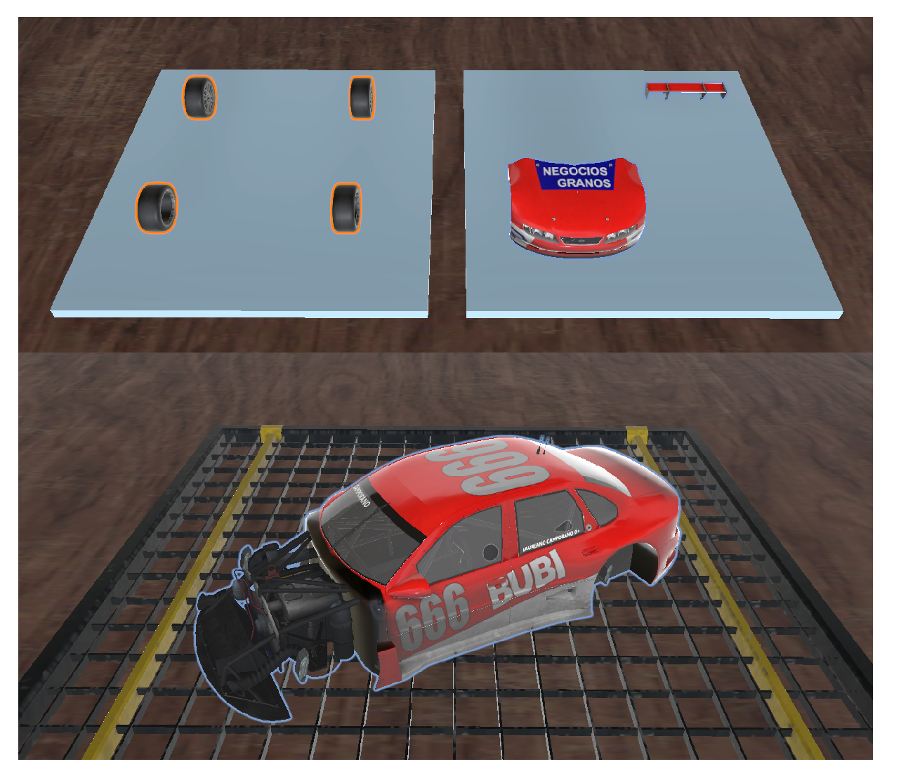
Figure 2.
Scenario 1. The robot delivers the assembly component to the user’s hand. The magenta path is composed of two segments. The first segment corresponds to the motion from the robot’s initial position to the storage area, represented by the two gray rectangles on the left side of each scene. The second segment corresponds to the motion from the storage area to the delivery point, which—depending on the scenario—may be the user’s hand, the light-blue zone, or the light-green zone.
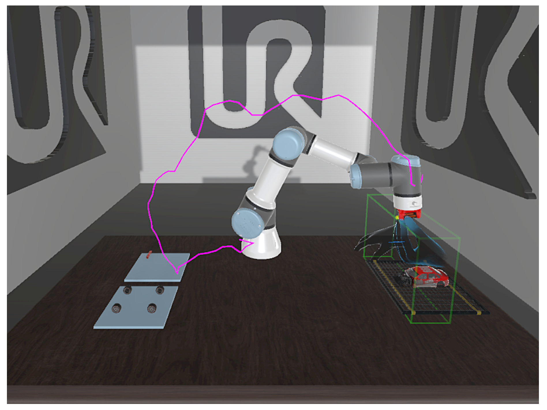
Figure 3.
Scenario 2. The robot places the assembly component on the light-blue zone.
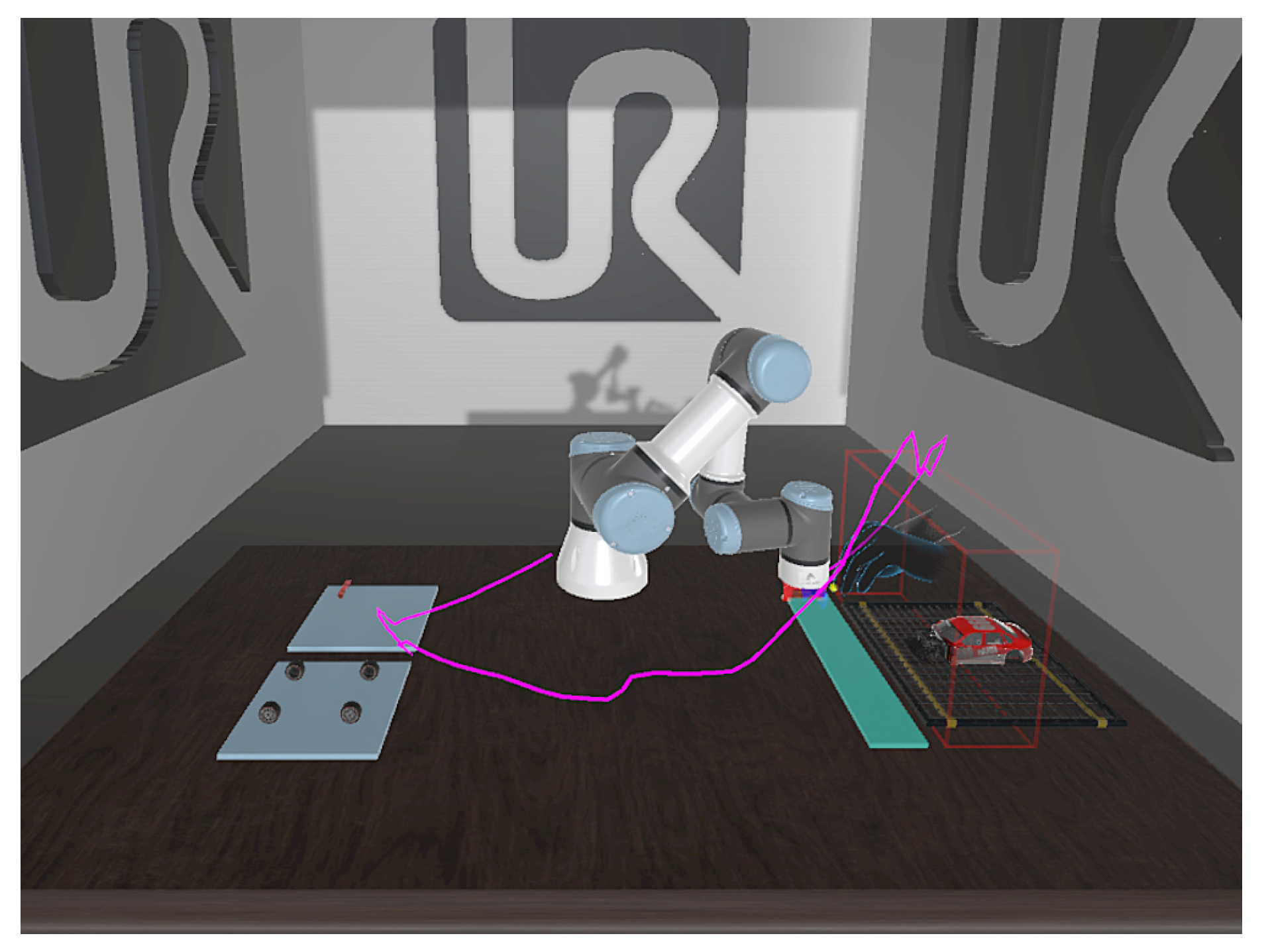
Figure 4.
Scenario 3. The robot places the assembly component on the light-green zone.
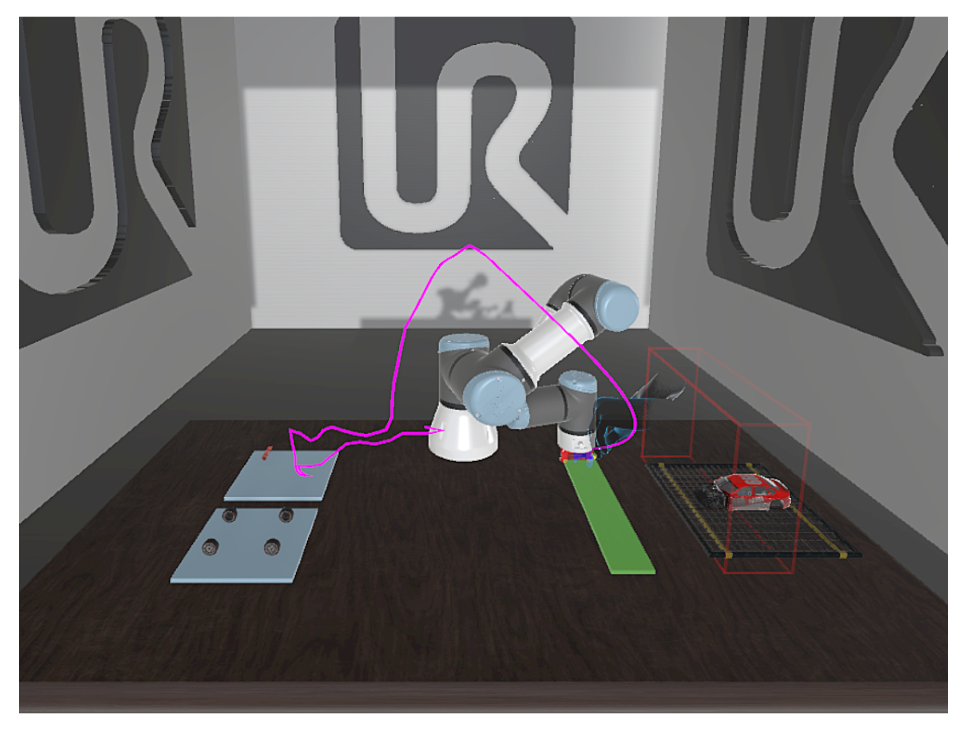
Figure 5.
Position validation in URSim.

Figure 6.
State machine illustrating the 13 trajectories associated with the complete assembly task (, ). The notation denotes Assembly Component j (). For example, represents the trajectory from the Home position to the location of Assembly Component 1 (). Similarly, corresponds to the trajectory from the location of Assembly Component 2 () to the delivery location, which depends on the scenario considered (the user’s hand in Scenario 1, the light-blue zone in Scenario 2, and the light-green zone in Scenario 3). The same numbering convention is applied to the remaining trajectories.
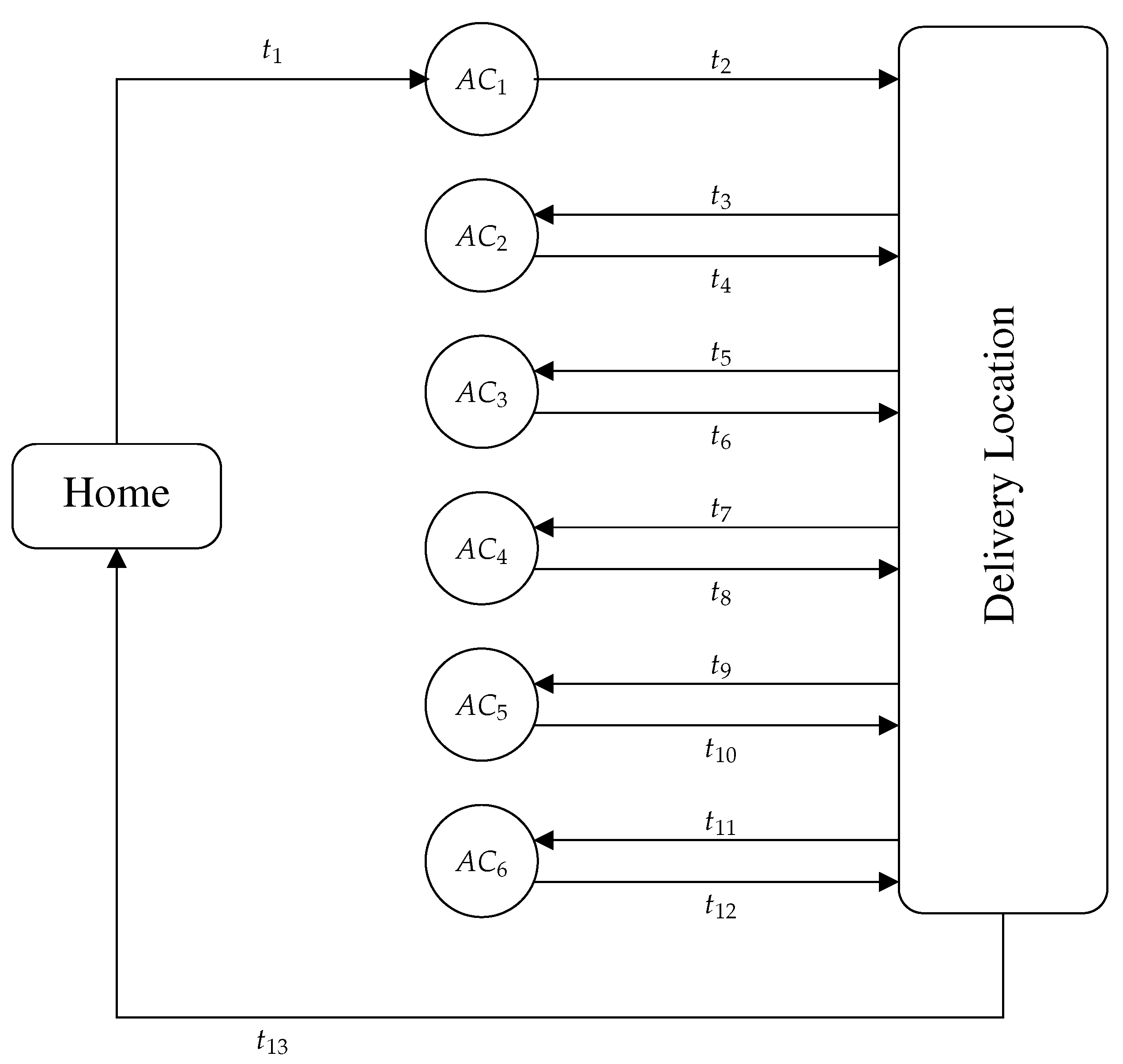
Figure 7.
Architecture of the trajectory planning system.
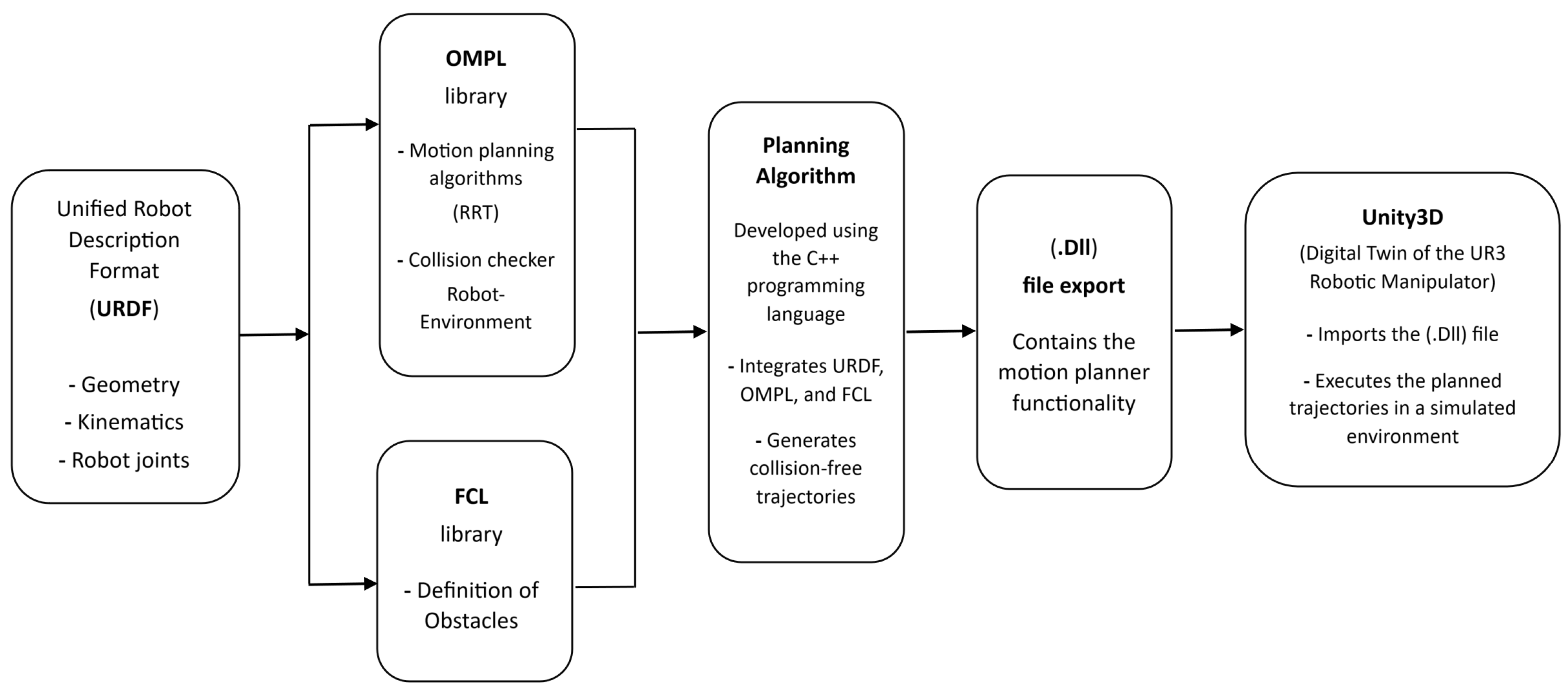
Figure 8.
Curvature by algorithm and scenario
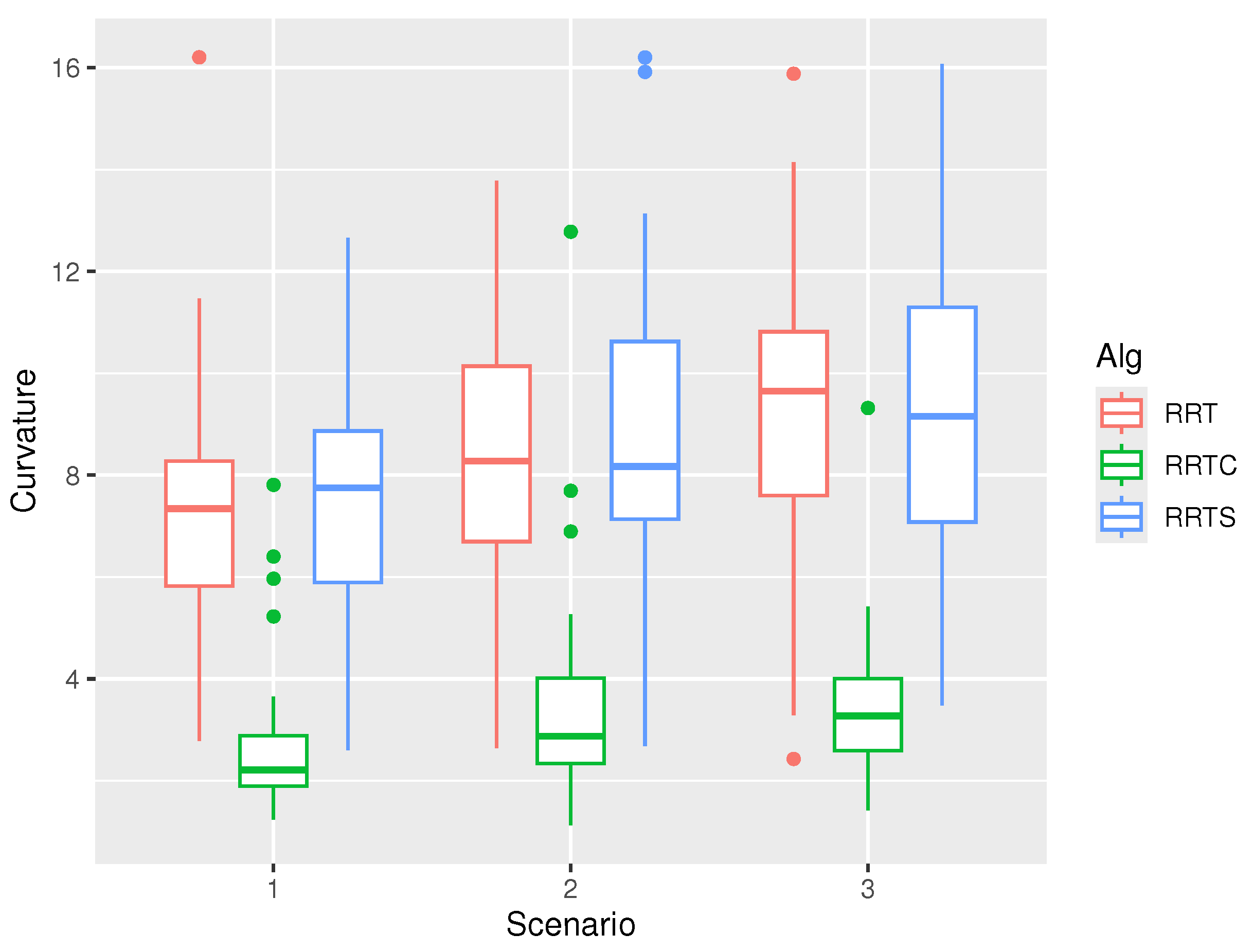
Figure 9.
Trajectory computation time by algorithm and scenario
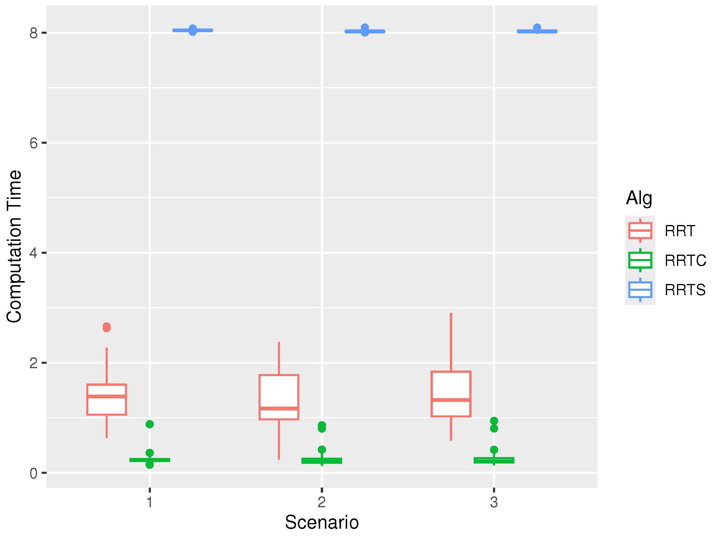

Table 1.
Saaty scale for pairwise comparisons in the Analytic Hierarchy Process.
| Score | Verbal judgment |
|---|---|
| 1 | Equal importance |
| 3 | Moderate importance |
| 5 | Strong importance |
| 7 | Very strong importance |
| 9 | Extreme importance |
| 1/3 | Moderate inverse importance |
| 1/5 | Strong inverse importance |
| 1/7 | Very strong inverse importance |
| 1/9 | Extreme inverse importance |
Table 2.
Three-factor ANOVA results for the curvature. The symbol : denotes interaction effects between the corresponding factors.
Table 2.
Three-factor ANOVA results for the curvature. The symbol : denotes interaction effects between the corresponding factors.
| Source | Sum Sq | Df | F value | Pr(>F) |
|---|---|---|---|---|
| (Intercept) | 15816.4 | 1 | 3125.3191 | |
| Alg | 2159.8 | 2 | 213.3890 | |
| Scenario | 148.5 | 2 | 14.6676 | |
| Trajectory | 317.1 | 12 | 5.2213 | |
| Alg : Scenario | 17.1 | 4 | 0.8441 | 0.4984 |
| Alg : Trajectory | 168.8 | 24 | 1.3898 | 0.1124 |
| Trajectory : Scenario | 153.1 | 24 | 1.2605 | 0.1928 |
| Alg : Scenario : Trajectory | 296.3 | 48 | 1.2198 | 0.1702 |
| Residuals | 1184.2 | 234 |
Table 3.
Difference of the mean trajectory curvature for each pair of algorithms. The second column indicates the difference between the mean curvature of two algorithms.
Table 3.
Difference of the mean trajectory curvature for each pair of algorithms. The second column indicates the difference between the mean curvature of two algorithms.
| Algorithm | Difference | Significance (p) |
|---|---|---|
| RRTC - RRT | -5.1742 | ≤ 0.0001 |
| RRTS - RRT | 0.1716 | 0.8291 |
| RRTS - RRTC | 5.3458 | ≤ 0.0001 |
Table 4.
Difference of the mean trajectory curvature for each scenario.
| Scenario | Difference | Significance (p) |
|---|---|---|
| 2 - 1 | 1.0658 | 0.0010 |
| 3 - 1 | 1.5582 | ≤ 0.0001 |
| 3 - 2 | 0.4924 | 0.2173 |
Table 5.
Difference of the mean curvature for each trajectory.
| Trajectory | Difference | Significance (p) |
|---|---|---|
| 4 - 1 | -3.1467 | ≤ 0.0001 |
| 5 - 1 | -2.3131 | 0.0188 |
| 6 - 1 | -3.3221 | ≤ 0.0001 |
| 7 - 1 | -2.4351 | 0.0096 |
| 8 - 1 | -2.9213 | 0.0004 |
| 9 - 1 | -2.8033 | 0.0010 |
| 10 - 1 | -2.9191 | 0.0004 |
| 11 - 1 | -2.3332 | 0.0169 |
| 12 - 1 | -3.4343 | ≤ 0.0001 |
| 13 - 1 | -3.9607 | ≤ 0.0001 |
| 13 - 3 | -2.1899 | 0.0355 |
Table 6.
Average curvature values and normalized smoothness performance for each algorithm.
| Algorithm | Average | Normalized | Smoothness |
|---|---|---|---|
| curvature | Value | performance | |
| RRT | 8.38 | 0.980 | 0.0201 |
| RRTC | 3.21 | 0.375 | 0.6250 |
| RRTS | 8.55 | 1.000 | 0.0000 |
Table 7.
Three-factor ANOVA results for trajectory computation time.
| Source | Sum Sq | Df | F value | Pr(>F) |
|---|---|---|---|---|
| (Intercept) | 3667.4 | 1 | 44065.5205 | |
| Alg | 4120.9 | 2 | 24757.8536 | |
| Scenario | 0.1 | 2 | 0.7466 | 0.4751 |
| Trajectory | 3.7 | 12 | 3.7351 | |
| Alg : Scenario | 0.3 | 4 | 0.7649 | 0.5490 |
| Alg : Trajectory | 5.6 | 24 | 2.8238 | |
| Scenario : Trajectory | 2.2 | 24 | 1.1125 | 0.3307 |
| Alg : Scenario : Trajectory | 4.1 | 48 | 1.0216 | 0.4425 |
| Residuals | 19.5 | 234 |
Table 8.
Average computation time and normalized performance for each algorithm.
| Algorithm | Average Time | Normalized Value | Time Performance |
|---|---|---|---|
| RRT | 1.41 | 0.1760 | 0.8240 |
| RRTC | 0.254 | 0.0316 | 0.9684 |
| RRTS | 8.03 | 1.0000 | 0.0000 |
Table 9.
Score–comparison between criteria.
| Comparison | Expert Judgment (Bibliographic Evidence) | Score |
|---|---|---|
| Safety vs Feasibility |
In CHR systems, safety is essential because motion planning must ensure collision-free trajectories to protect the operator [45,46]. While feasibility is necessary, a trajectory loses practical value if it does not guarantee safe conditions [13]. Moreover, geometrically feasible trajectories can still pose risks in complex environments [49,50]. Therefore, safety was judged strongly more important than feasibility. | 5 |
| Safety vs Smoothness |
Smoothness improves predictability and comfort [13,48], but it does not prevent collisions, since smooth trajectories may still pass dangerously close to humans or obstacles [50,51]. Therefore, safety was judged very strongly more important than smoothness. | 7 |
| Safety vs Computation time |
Computational efficiency should not compromise safety in collaborative robotics [46,48]. Planning-time reductions are irrelevant if they lead to unsafe trajectories [30,52]. Thus, safety was judged extremely more important than computation time. | 9 |
| Feasibility vs Smoothness |
Feasibility ensures the trajectory remains within joint limits, which must be satisfied before evaluating other criteria [13]. Smoothness improves interaction quality [47,48], but a smooth trajectory that is unreachable is unusable. Therefore, feasibility was judged moderately more important than smoothness. | 3 |
| Feasibility vs Computation time |
A trajectory must be executable within joint limits before considering computation time [13]. Faster algorithms may be less reliable in complex scenarios [50]. Therefore, feasibility was judged strongly more important than computation time. | 5 |
| Smoothness vs Computation time |
Smoothness improves HRI by reducing abrupt movements and lowering cognitive load [13,48]. Achieving smoother trajectories may require additional computation, which is acceptable when interaction quality is prioritized [50,51]. Therefore, smoothness was judged moderately more important than computation time. | 3 |
Table 10.
Criteria comparison matrix and resulting weights.
| Criteria | S | F | T | M | ||
|---|---|---|---|---|---|---|
| S | 1 | 5 | 7 | 9 | 4.2129 | 0.6545 |
| F | 1/5 | 1 | 3 | 5 | 1.3161 | 0.2045 |
| 1/7 | 1/3 | 1 | 3 | 0.6148 | 0.0955 | |
| T | 1/9 | 1/5 | 1/3 | 1 | 0.2934 | 0.0456 |
| Total (sum of geometric means) | 6.4371 | 1 | ||||
Disclaimer/Publisher’s Note: The statements, opinions and data contained in all publications are solely those of the individual author(s) and contributor(s) and not of MDPI and/or the editor(s). MDPI and/or the editor(s) disclaim responsibility for any injury to people or property resulting from any ideas, methods, instructions or products referred to in the content. |
© 2026 by the authors. Licensee MDPI, Basel, Switzerland. This article is an open access article distributed under the terms and conditions of the Creative Commons Attribution (CC BY) license (http://creativecommons.org/licenses/by/4.0/).
Copyright: This open access article is published under a Creative Commons CC BY 4.0 license, which permit the free download, distribution, and reuse, provided that the author and preprint are cited in any reuse.


