
Submitted:
09 February 2026
Posted:
10 February 2026
You are already at the latest version
Abstract
Buildings located in highly urbanized areas have not been considered for photovoltaic (PV) deployment on building walls due to limitation of ground and rooftops space. As the need for increasing energy demand due to population growth in cities, and the advancements in the efficiency of semi-transparent (ST-PV) solar cell technology, the integration of ST-PV modules into building windows, become feasible. The present article proposes a novel methodology for calculating the incident solar energy on PV vertical modules deployed on building walls and windows facing the southern direction and obscured by a nearby building in front. The present work analyses analytically, for the first time, the incident energy and its distribution on PV vertical modules along a wall height. Monthly and annually direct beam, diffuse and global energies are calculated for different wall height, building separation and orientation. The results shows, for example, that both the front and rear building walls receive the same amount of annual direct beam energy 913 kWh/m2 for a distance 25 m between the buildings. Decreasing the distance from 25 m to 10 m, decreases the annual incident global energy on the rear-building wall by 15 %.
Keywords:
PV in urban area
; PV on building walls
; window PV
; ST-PV modules
; incident solar energy
1. Introduction
The deployment of solar photovoltaic (PV) systems on rooftops, building walls and building windows in urban environments is to utilize potential land area for electricity generation. This approach also matches the need for increasing demand of energy due to population growth in cities. In addition, the generated electric energy at the site where the energy is demanded, avoids long and expensive transmission lines from electric power stations to the urban areas. Buildings located in highly urbanized areas have not been considered in the past for PV deployments due to limitation of ground and rooftops space [1]. These days, PV modules integrated into walls and windows becomes a prospective technology for reasons mentioned above. PV opaque modules may be deployed on building walls, and semi-transparent PV (ST-PV) modules may be deployed on building windows. Mono-facial PV modules is a well established technology, whereas ST-PV technologies are still under development, including organic, dye synthesized, polymer- and perovskite-based solar cells [2]. A comparison of three technologies (c-Si, CIS and CdTe), for building application under tropical weather conditions, employing the PVGIS tool, is in [3]. The present article proposes a novel methodology for calculating the incident solar energy on PV vertical modules of building walls obscured by a nearby building in front. The two vertical buildings are separated by a road and facing the southern direction. As the purpose is to calculate the incident solar radiation on the PV vertical modules, no distinction is made between walls and windows. The monthly and annually incident direct beam, diffuse and global energies are determined for a front unshaded building wall and on an obscured rear shaded building wall for different building height, building separation and building orientation. The uniformity of the incident solar energy on the PV modules along the height of the obscured building wall is numerically demonstrated, for the first time. The non-uniformity stems basically from the incident diffuse radiation rather from the mutual collector shading, for the examined buildings walls dimensions and the site location. The term “wall” means building-wall, front wall or unshaded wall means the building-wall on the left, and rear wall or shaded wall means the building-wall to the right, see Figure 1.
2. Methods and Materials
Geometry. Figure 1 depicts window PV collectors positioned on vertical () walls of two buildings and separated by a road, in an urban environment. The buildings erected in east-west direction of length and walls facing the south. The height of the front (left) and rear (right) walls is and , respectively. Because the walls are assumed relatively long, Hottel’s cross-string rule [4] is used to evaluate the view factor of the walls to sky. As the purpose is to calculate the incident solar energy on the vertical PV modules, no distinction is made between walls and windows.
2.1. Incident Direct Beam Radiation
2.1.1. Left Wall
The incident direct beam radiation on the front wall is given by:
where is the direct beam irradiance, is the angle between solar rays and the normal to the wall surface. The angle is given by:
where is the wall azimuth angle (walls facing due south) and is the solar azimuth angle.
2.1.2. Right Wall
The incident direct beam radiation on the right wall is given by:
The shadow height and length on the right wall caused by the front wall , is given by the following [5]:
where is the wall shading area, .
For a vertical wall, Eqs.(4) and (5) reduce to:
and Eq.(2) becomes
The incident solar energy on a wall is integrated for the duration of the solar rays impinges the wall, and depends on the sunrise and sunset hour angles and on the inclination angleof the collector. The hour angle for which the sun starts climbing on the wall (wall rise) , and leaving the wall (wall set) , is given by [6]:
The upper sign is valid for eastward-orientated walls, and the lower sign for westward- oriented walls, where:
For collector inclination angle, Eq.(13) reduces to:
The sunrise and sunset hour angles ,, respectively is given in [6],
The sunrise and sunset hour angles on an inclined plane denoted by (wall rise) and (wall set) are as follows:
and for ,
Therefore, the sunrise and sunset hours on a wall is thus determined by:
2.2. Incident Diffuse Radiation
The incident diffuse radiation on a wall, for isotropic diffuse radiation model, is given by:
where is the view factor of the wall to sky, and is the diffuse radiation on a horizontal plane. The sky view factor of an inclined wall in open space (front building wall, see Figure 1) is [7]:
and for , The sky view factor of a vertical wall,, deployed behind a front wall, (see Figure 1) is given by [4], see Figure 2:
i.e.,
2.3. Local Sky View Factor
The view factor of a collector (wall) to sky is an “average” view factor of the entire collector (wall) to sky. However, the sky view factor varies with the distance along the heightof the wall denoted as “local” sky view factor. The collectors on the rear-building wall comprises modules forming parallel segments/stripes along the wall length. Each segment sees the sky with a different angle, hence a different local sky view factor is attached to each segment,, see Figure 3. The local sky view factors, based on Eq.(21) and Figure 3, is determined for N parallel segments, by:
where As the diffuse incident irradiance is connected to sky view factor (see Eq.(19)) , the diffuse incident irradiance on wall becomes non-uniform.
3. Results
The monthly and the annual energies, in , of the incident direct beam, diffuse and global radiation on collectors deployed on building walls are analyzed for different wall height, distance between the building wall and wall orientation, including the non-uniformity of the energies along the wall height of . The incident solar radiation on walls is based on 10 minutes solar radiation data (direct beam and diffuse radiation, average data for years 2014-2023) , Israel, Meteorological Service–IMS) for Tel Aviv, latitude, longitude.
3.1. Distance Between Walls,(Front Wall Lower than Rear Wall),
The incident direct beam radiation depends strongly on the angle between solar rays and the normal to the wall surface, Eq.(2). Figure 4 depics the variation of with time of the day for specific four months on 21st of December, April, June and September, for a avertical wall, and considering the times the sunbeam impinges the collector ( see Eq.(18). The figure clearly shows that the lowest value of is in June. Consequently, Figure 5 shows the monthly incident direct beam energy on the walls - front (left) wall - unshaded in red, and rear (right) wall – shaded in blue, based on Eqs.(1) and (3), for parameters , and buildings facing the south (see Figure 1). Lower energies is obtained in summer months as the effect of dominates the resulted energies, see Eqs.(1), (3) and Figure 4. Figure 5 shows that for a relative large distance between the building walls, no shading occurs on the rear building wall caused by the front building, i.e., both building walls receives the same amount of direct beam energy.
Figure 4 and Figure 5 show that the incident solar energy on southern building walls is relatively low in summer months, thus saving cooling energy. The opposite is in winter months, solar energy on the buildubg walls is heigher, and thus saving heating energy.
Figure 6 depicts the monthly incident diffuse energy on the front (left) wall, in red, and on the rear (right) wall, in blue, for parameter(see Figure 1).
The sky view factor of the front building wall is larger than the sky view factor of the rear building wall, (see Eqs. (20), (22)), and accordingly are the incident diffuse energies. The global incident energy is the sum of the direct beam and the diffuse energies. Decreasing the distance between the buildings to causes shading on the rear-building wall by the front building. This is shown in Figure 7 for the incident direct beam energy. The incident diffuse and global energies act accordingly.
Table 1 shows the annual incident direct beam, diffuse and global energies, in, on the front and rear building walls for different distances between the building. Both the front and rear walls receive the same amount of annual direct beam energy for the distance. However, the diffuse and global energies on the rear wall are less by 19.19% and 5.88%, respectively. Decreasing the distance from 25 m to 10 m decreases the annual incident direct beam, diffuse and global energies on the rear wall by 10.55%, 27.5% and 15.5%, respectively.
3.2. Distance Between the Building Walls, (Front Building Higher than Rear Building),
Figure 8 depicts the monthly incident direct beam energy on the front (unshaded) wall in red, and on the rear (shaded) wall in blue, for parameters (see Figure 1). The rear-building wall suffer shading in Jan., Nov., and Dec. months only. Figure 9 depicts the monthly incident diffuse energies. The masking losses (diffuse radiation losses) on the rear wall are more noticeable than for the front wall, resulting from the difference in the sky view factors.
Table 2 shows the annual incident direct beam, diffuse and global energies, in , on the front and rear building walls, for wall height and, both forand. The front and rear walls receive the same amount of annual direct beam energy for . However, the diffuse and global energies on the rear wall are less by 36.58% and 11.25%, respectively. Increasing the wall height to decreases the annual incident direct beam, diffuse and global energies on the rear wall by 4.26%, 50.67% and 18.40%, respectively.
3.3. Building Walls Oriented with Azimuth Angle
Buildings may be constructed with any azimuth angle with respect to south. This section deals with incident monthly and annually energies on building walls oriented with azimuth angle, as a compared to walls with, Table 1. The results are shown in Table 3.
The values and remain the same and the distance beween the building are: .
The global energy on the rear wall is less than on the front wall by 7.07% for .Decreasing the distance from 25 m to 10 m decreases the annual incident direct beam, diffuse and global energies on the rear wall by 15.72%, 27.5% and 18.71%, respectively. By comparing Table1 () and Table 3 () for, the global energies on the rear wall as compared to the front wall are less by 5.88% and 7.07%, respectively.
.
3.4. Local Sky View Factor
The sky view factor varies with the distance along the heightof the building wall (see Section 2.3). The wall height,, is divided intosegments (strips) corresponding of the PV module height. The sky view factor of each segment, denoted by “local” sky view factor, varies with wall height. Figure 10 shows the variation of the local sky view factor with segment number for, as an example. The segment height is. As the diffuse incident irradiance is associated to sky view factor (see Eq.(19)) , the distribution of the incident diffuse energy on the segments becomes noticeable non-uniform. Table 4 shows the distribution of the monthly direct beam energy on the segments of for parameters, and building length.
The darker areas in Table 4 indicate that the shadows occurred on the segments in winter months, for example, in December, the shadow height reached segment 6. The annual total direct beam energy on each segment is listed in the last line, and its distribution is depicted in Figure 11, indicating that segments 1 and 2 (both of height 2 m), located at the bottom of the right wall, suffer substantial shading.
The distribution of the annual incident diffuse energy on the segments, is depicted in Figure 12, indicting a broad uneven distribution of the diffuse energy on the segments, stemming from the large variation of the sky view factors, see Figure 10. The distribution of the annual incident global energy on the segments is depicted in Figure 13, indicating a variation in the incident global energy on the segments, mainly affected by the diffuse radiation. The difference in the annual incident global energy between the first and eight segment is about 50 %.
The results presented in this section pertain to the solar radiation data for location, latitude, longitude. Different results may be obtained for different location sites, however the variation of the sky view factor along the height of a building wall dictates the non-uniformity of the incident global energy on the different segments of the PV modules deployed on the wall.
4. Discussion
The deployment of solar photovoltaic (PV) modules on building walls and windows in urban environment is to utilize potential area for electricity generation to alleviate the need for increasing demand for energy due to population growth in cities. PV modules integrated into windows becomes a prospective technology, these days, due to advancements in the efficiency of semi-transparent (ST-PV) solar cell technology. Buildings constructed in urban areas and separated by alleys and roads, are facing each other and therefore may obscure the solar beam from reaching the building walls. To determine whether PV modues installations on walls are viable, the incident solar energy on the walls are needed to assess. The present article proposes a novel methodology for calculating the incident solar energy of PV vertical modules on building walls/windows obscured by a nearby building in front. Monthly and annually direct beam, diffuse and global energies are calculated on a front-building wall and on a rear-building wall for different wall height, building separation and orientation. The results show that the solar energy on walls facing the south, is relatively low in summer months, thus may saving cooling energy, and in winter, the solar energy on the walls is heigher, and thus may saving heating energy. This results pertain to sites of relatively low latitudes. Local sky view factors of the obscured building wall segments, are mathematically formulated and calculated, to determine the uniformity of the global incident radiation along the height of the rear-building wall. The obtained non-uniformity stems from the different local sky view factors and hence, from the incident diffuse energy on the different segments. It is worth mentioning that the sky view factor is independent on the buildings location and orientation, but depends on the dimensions of the buildings and the separation.
5. Conclusion
Buildings located in highly urbanized areas have not been considered, in the past, for PV deployment on walls due to limitation of ground and rooftops space. These days, PV vertical modules integrated into walls and windows becomes a prospective technology due to the increase in module efficiency. The present article proposes a novel methodology for calculating the incident solar energy on PV vertical modules deployed on a building walls obscured by a nearby buildings in front. The buildings are separated by a roads and facing the southern direction. The work calculates, for the first time, the incident energy and its distribution along the height of an obscuring building wall. Monthly and annually direct beam, diffuse and global energies are calculated for different wall height, building separation and orientation. The results shows, for example, that both the front and rear building walls receive the same amount of annual direct beam energy for a distance 25 m between the buildings. Decreasing the distance from 25 m to 10 m, decreases the annual incident global energy on the rear-building wall by 15 %. The results pertain to the solar radiation data at location, latitude, longitude, and for building height and separation dealt in the article. Different results may be obtained for different location sites and different building dimensions.
Nomenclature
Front building wall heightm
Rear building wall heightm
Shadow height on rear wallm
Direct beam irradiance W/m2
Incident direct beam radiation W/m2
Diffuse radiation on a horizontal plane W/m2
Wall length m
Shadow length on rear wall m
Wall shading aream2
Sky view factor of front wall
Sky view factor of rear wall
Solar altitude angledeg.
Collector inclination angle deg.
Sun declination angle deg.
Collector latitude, deg.
Collector azimuth angledeg.
Solar azimuth angle- deg., forenoon afternoon
Angle between solar rays and the normal to wall surfacedeg.
Solar zenith angle - deg.
Sunrise hour anglesdeg.
Sunset hour angledeg.
Collector rise hour abgledeg.
Collector set hour angledeg.
References
- Panagiotidou, M.; Brito, M.C.; Hamza, K.; Jasieniak, J.J.; Zhou, J. Prospects of photovoltaic rooftops, walls and windows at a city building scale. Solar Energy 2021, 230, 675–687. [Google Scholar] [CrossRef]
- Lee, K.; Um, H.-D.; Choi, D.; Park, J.; Kim, N.; Kim, H.; Seo, K. The development of transparent photovoltaics. Cell Reports Phys. Sci 2020, 1(8), 100143. [Google Scholar] [CrossRef]
- Kumar, N.M.; Sudhakar, K.; Samykano, M. Performance comparison of BAPV and BIPV systems with c-Si, CIS and CdTe photovoltaic technologies under tropical weather conditions. Case Stud. Therm. Eng. 2019, 13, 100374. [Google Scholar] [CrossRef]
- Hottel, H.C.; Sarofin, A.F. Radiative Transfer; McGraw-Hill: New York, NY, USA, 1967; pp. 31–39. [Google Scholar]
- Bany, J.; Appelbaum, J. The effect of shading on the design of a field of solar collectors. Sol. Cells 1987, 20, 201–228. [Google Scholar] [CrossRef]
- Duffie, J.A.; Beckman, W.A. Solar engineering of thermal processes; Wiley: London, 1974; ISBN 0-471-22371-9. [Google Scholar]
- Liu, B.Y.H.; Jordan, R.C. The long-term average performance of flat-plate solar energy collectors. Sol. Energy 1963, 7, 53–74. [Google Scholar] [CrossRef]
Figure 1.
Window PV modules in urban environment.
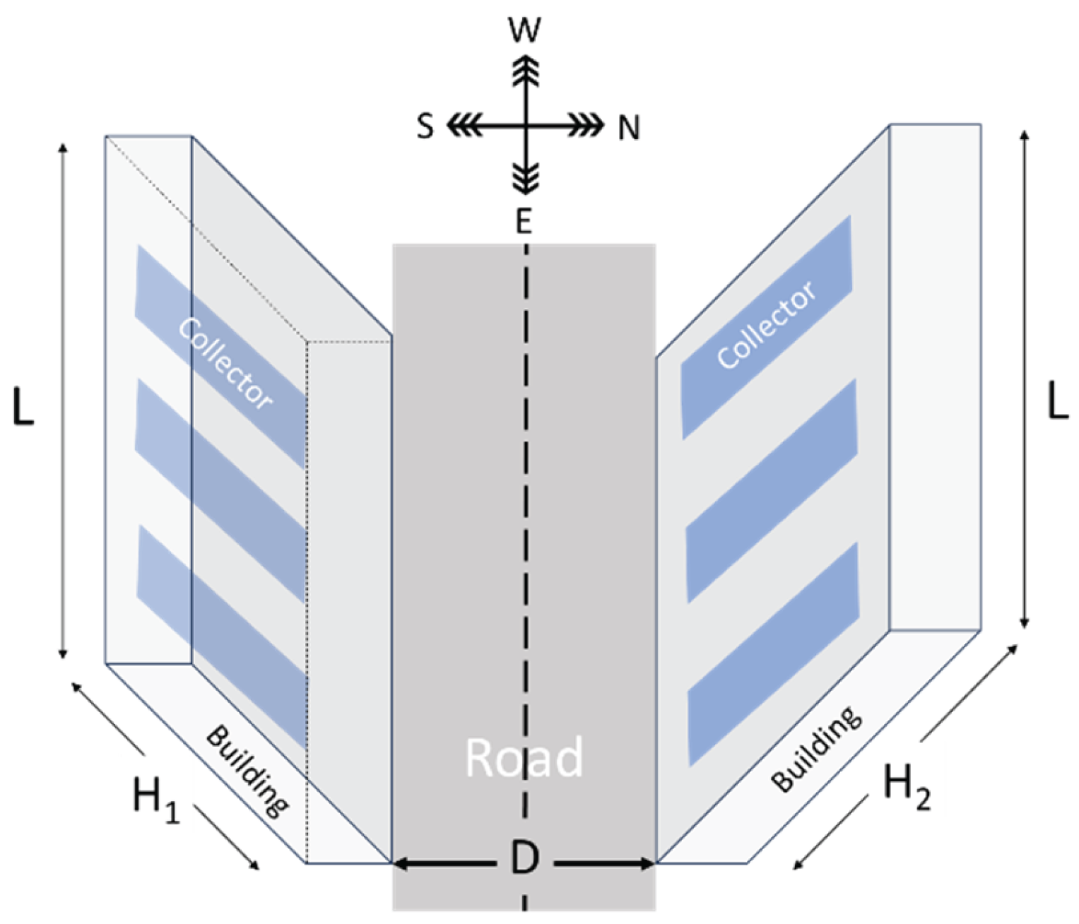
Figure 2.
- Sky view factor, Eq.(22).
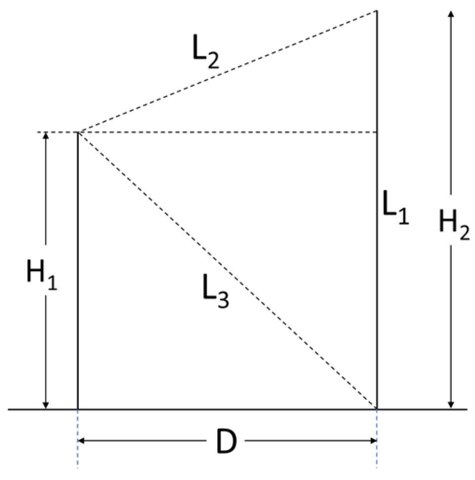
Figure 3.
Local view factors.
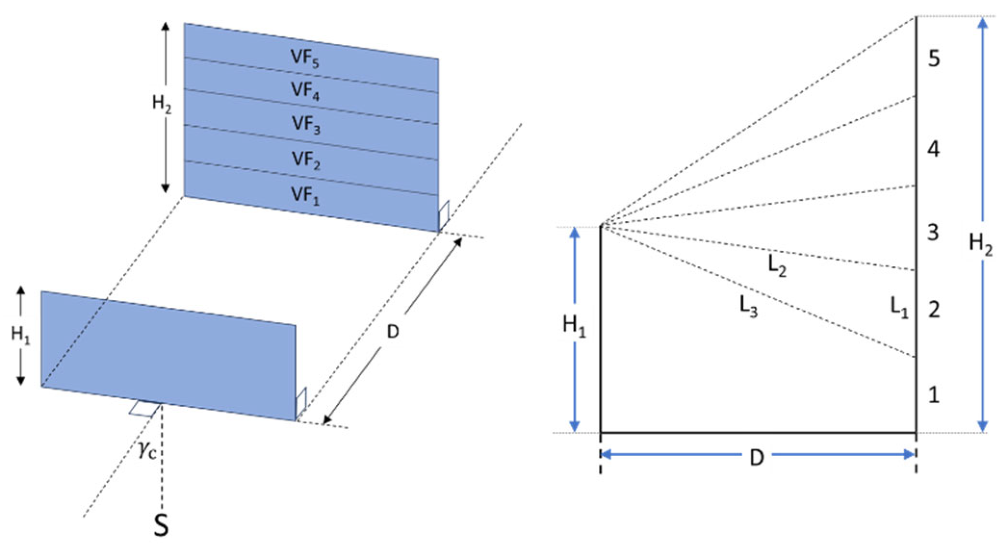
Figure 4.
Variation of with time of day for 21st Dec., April, June, Sep.,.
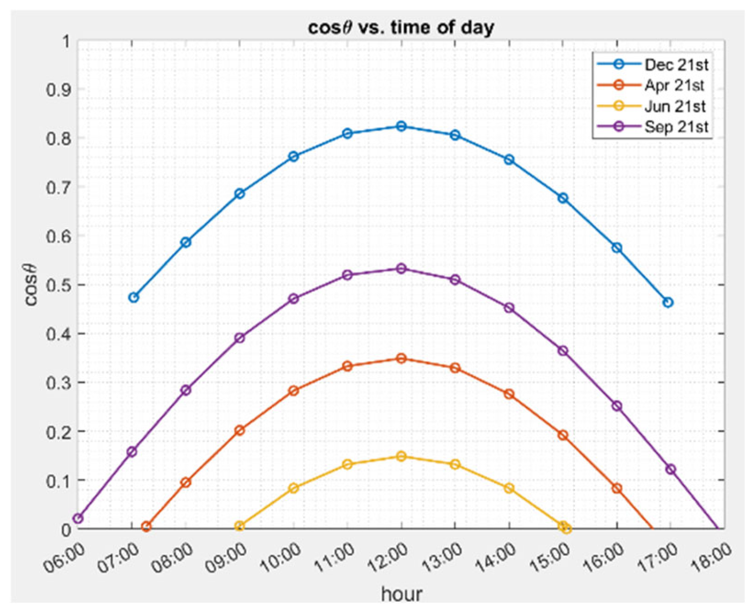
Figure 5.
Monthly incident direct beam energy for.
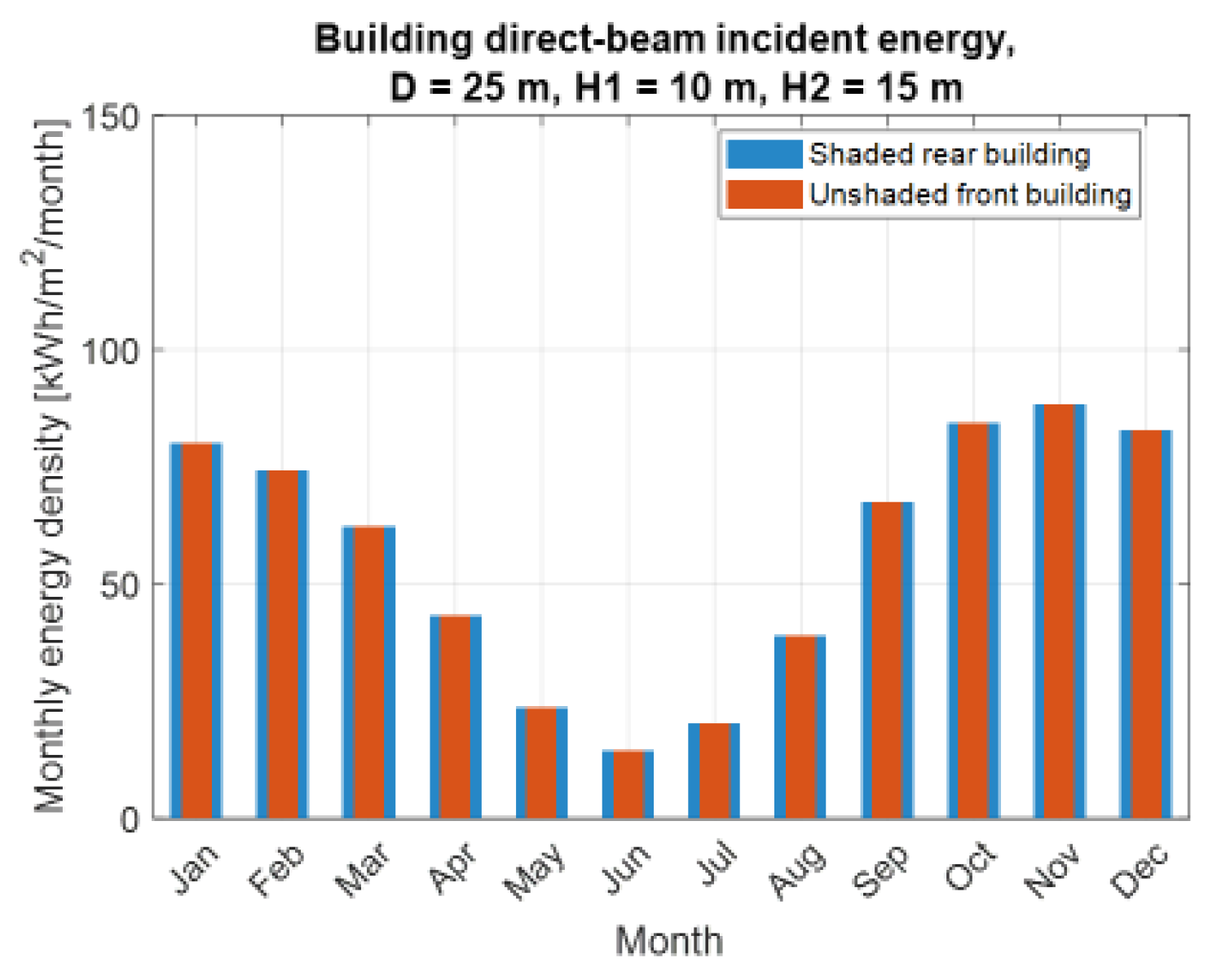
Figure 6.
Monthly incident diffuse energy.
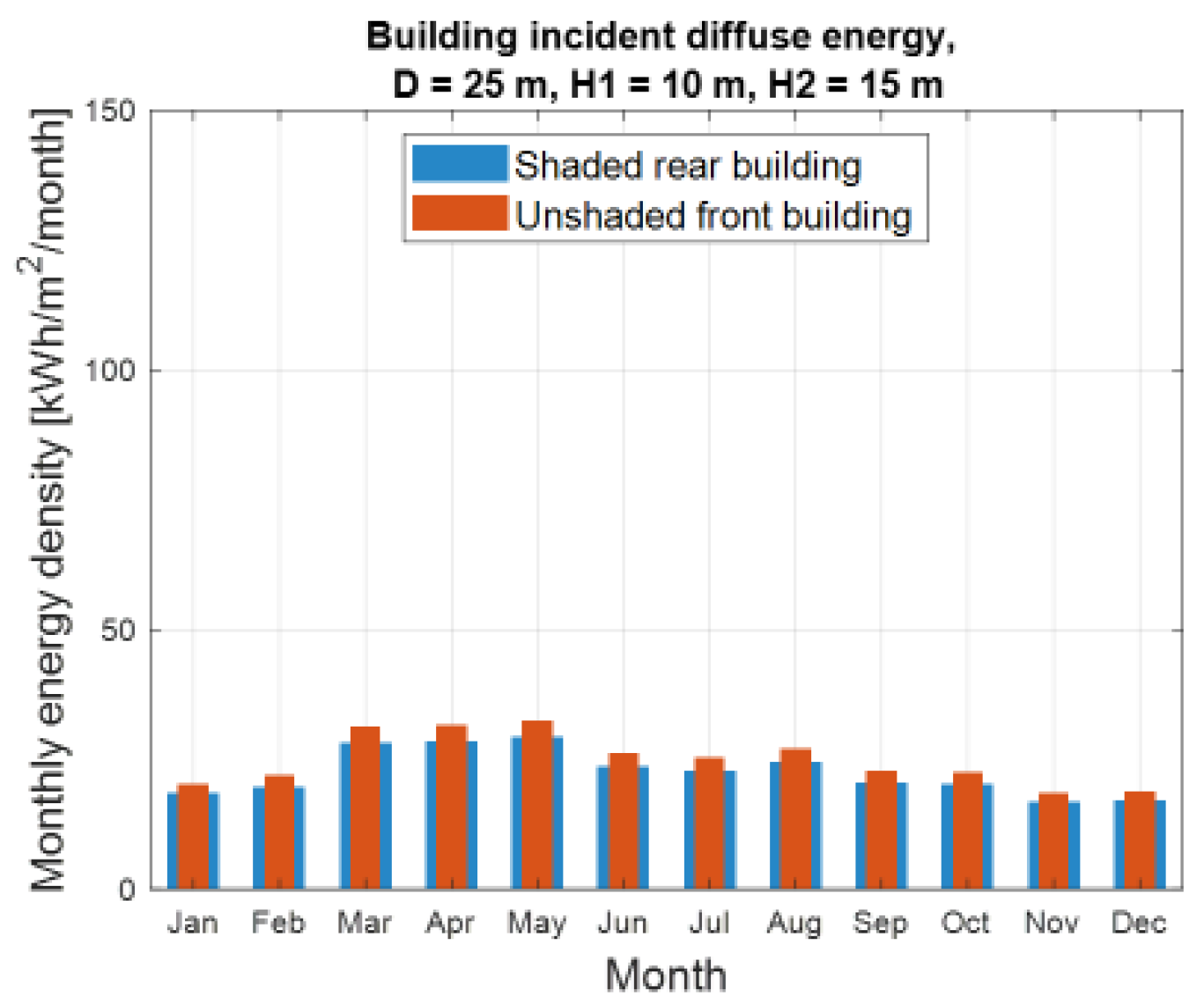
Figure 7.
Monthly incident direct beam energy for.
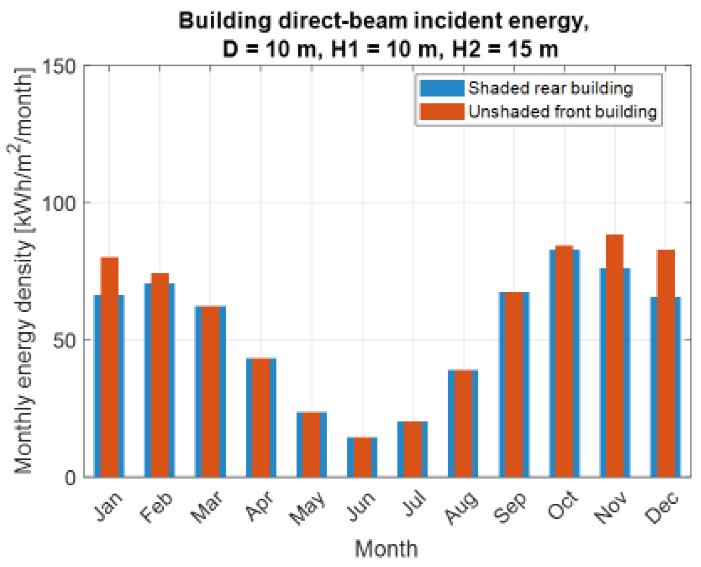
Figure 8.
Monthly incident direct beam energy for.
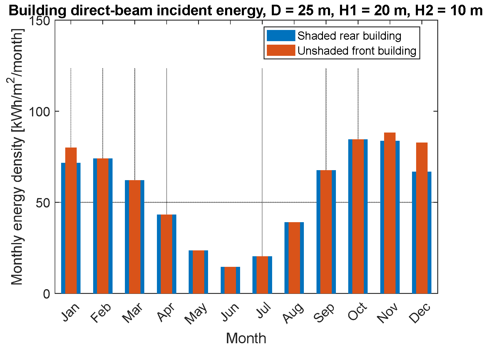
Figure 9.
Monthly incident diffuse energy for.
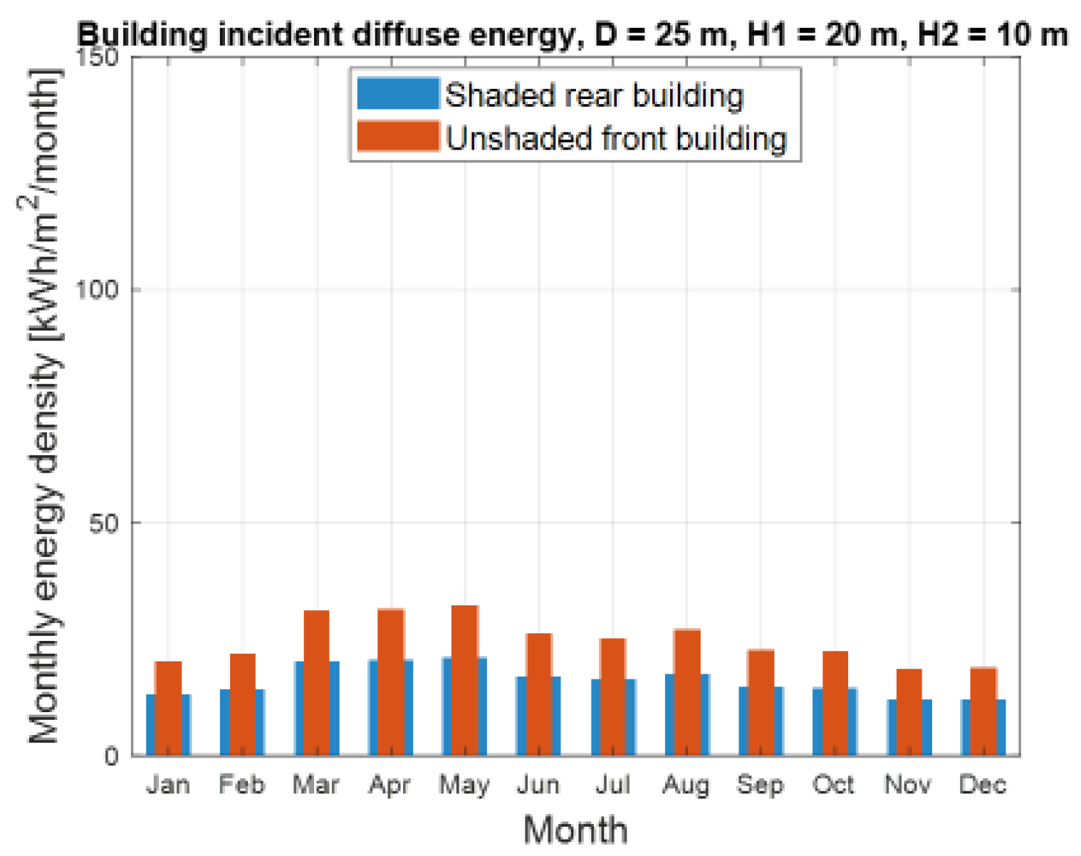
Figure 10.
Variation of local sky view factor with segment number , Eq.(23).
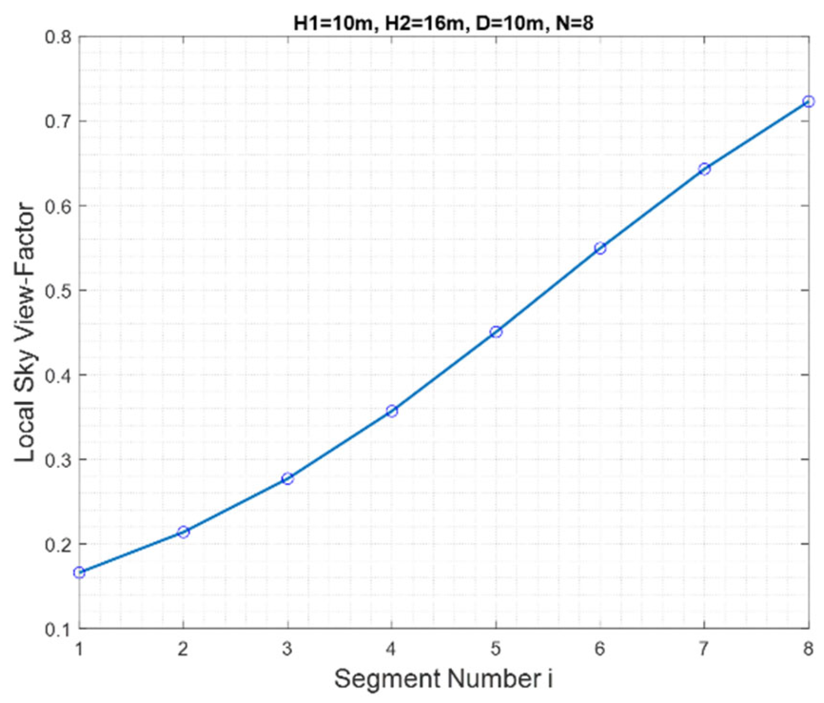
Figure 11.
Distribution of annual incident direct beam energy on segments.
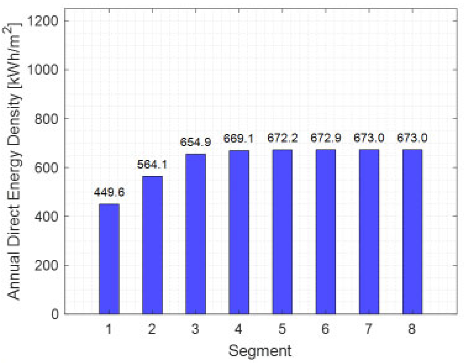
Figure 12.
Distribution of annual incident diffuse energy on segments.
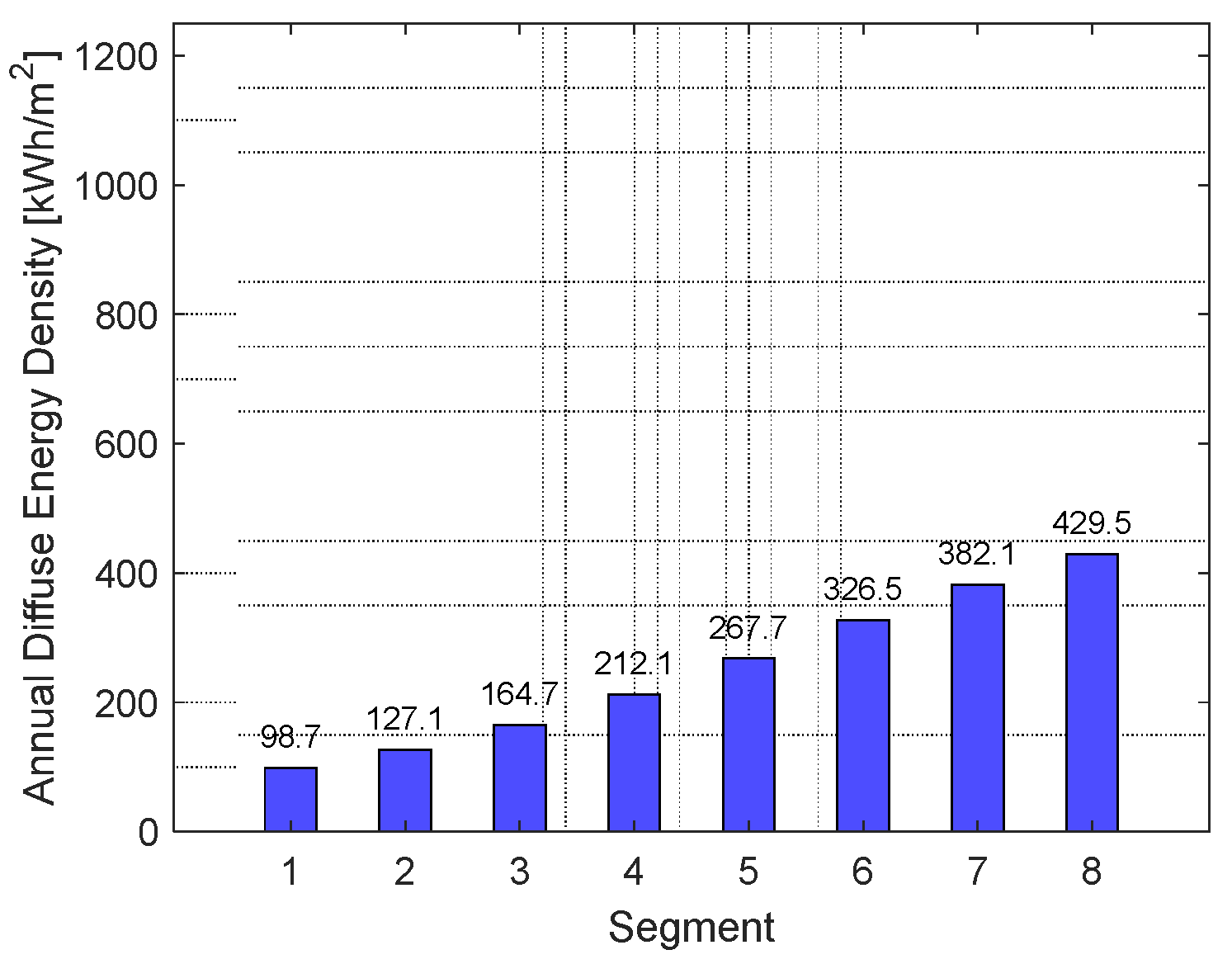
Figure 13.
Distribution of annual incident global energy on segments.
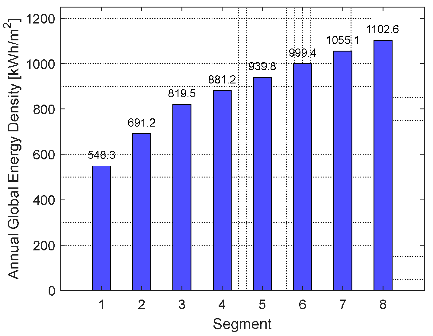

Table 1.
Direct beam, diffuse, global energies - variation in distance between buildings.
| Beam [kWh/m2/year |
Diffuse [kWh/m2/year |
Global [kWh/m2/year |
|
|---|---|---|---|
| Rear collectors, H1=10 m, H2=15 m, D=25 m | 673 | 240 | 913 |
| Rear collectors, H1=10 m, H2=15 m, D=15 m | 666 | 207 | 873 |
| Rear collectors, H1=10 m, H2=15 m, D=10 m | 602 | 174 | 776 |
| Front collectors, H1=10 m, H2=15 m, D=25 m | 673 | 297 | 970 |
| Front collectors, H1=10 m, H2=15 m, D=15 m | 673 | 297 | 970 |
| Front collectors, H1=10 m, H2=15 m, D=10 m | 673 | 297 | 970 |
Table 2.
Direct beam, diffuse, global energies - variation in wall height.
| Beam [kWh/m2/year |
Diffuse [kWh/m2/year |
Global [kWh/m2/year |
|
|---|---|---|---|
| Rear building, H1=15 m, H2=10 m, D=25 m | 680 | 189 | 868 |
| Rear building, H1=20 m, H2=10 m, D=15 m | 651 | 147 | 798 |
| Front building, H1=15 m, H2=10 m, D=25 m | 680 | 298 | 978 |
| Front building, H1=20 m, H2=10 m, D=25 m | 680 | 298 | 978 |
Table 3.
Direct beam, diffuse, global energies - variation in distance between buildings
| Beam [kWh/m2/ year |
Diffuse [kWh/m2/ year |
Global [kWh/m2/ year |
|
|---|---|---|---|
| Rear building, H1=10 m, H2=15 m, D=25 m | 706 | 240 | 946 |
| Rear building, H1=10 m, H2=15 m, D=15 m | 665 | 207 | 872 |
| Rear building, H1=10 m, H2=15 m, D=10 m | 595 | 174 | 769 |
| Front building, H1=10 m, H2=15 m, D=25 m | 721 | 297 | 1018 |
| Front building, H1=10 m, H2=15 m, D=15 m | 721 | 297 | 1018 |
| Front building, H1=10 m, H2=15 m, D=15 m | 721 | 297 | 1018 |
Table 4.
Direct beam energy on segments along .
| Month | Segment 1 [kWh/m2/ Month] |
Segment 2 [kWh/m2/ month] |
Segment 3 [kWh/m2/ Month] |
Segment 4 [kWh/m2/ month] |
Segment 5 [kWh/m2/ month] |
Segment 6 [kWh/m2/ month] |
Segment 7 [kWh/m2/ month] |
Segment 8 [kWh/m2/ month] |
|---|---|---|---|---|---|---|---|---|
| 1 | 16.62 | 46.51 | 72.90 | 77.45 | 78.15 | 78.48 | 78.48 | 78.48 |
| 2 | 50.63 | 69.30 | 72.32 | 72.74 | 72.90 | 72.90 | 72.90 | 72.90 |
| 3 | 61.80 | 61.85 | 61.85 | 61.85 | 61.85 | 61.85 | 61.85 | 61.85 |
| 4 | 43.00 | 43.00 | 43.00 | 43.00 | 43.00 | 43.00 | 43.00 | 43.00 |
| 5 | 23.23 | 23.23 | 23.23 | 23.23 | 23.23 | 23.23 | 23.23 | 23.23 |
| 6 | 14.31 | 14.31 | 14.31 | 14.31 | 14.31 | 14.31 | 14.31 | 14.31 |
| 7 | 20.03 | 20.03 | 20.03 | 20.03 | 20.03 | 20.03 | 20.03 | 20.03 |
| 8 | 38.73 | 38.73 | 38.73 | 38.73 | 38.73 | 38.73 | 38.73 | 38.73 |
| 9 | 67.36 | 67.36 | 67.36 | 67.36 | 67.36 | 67.36 | 67.36 | 67.36 |
| 10 | 74.13 | 82.69 | 83.94 | 84.11 | 84.11 | 84.11 | 84.11 | 84.11 |
| 11 | 24.65 | 64.81 | 83.64 | 86.78 | 87.34 | 87.46 | 87.51 | 87.51 |
| 12 | 15.15 | 32.30 | 73.56 | 79.48 | 81.14 | 81.46 | 81.53 | 81.53 |
| Total | 449.65 | 564.13 | 654.87 | 669.08 | 672.16 | 672.93 | 673.05 | 673.05 |
Disclaimer/Publisher’s Note: The statements, opinions and data contained in all publications are solely those of the individual author(s) and contributor(s) and not of MDPI and/or the editor(s). MDPI and/or the editor(s) disclaim responsibility for any injury to people or property resulting from any ideas, methods, instructions or products referred to in the content. |
© 2026 by the authors. Licensee MDPI, Basel, Switzerland. This article is an open access article distributed under the terms and conditions of the Creative Commons Attribution (CC BY) license (http://creativecommons.org/licenses/by/4.0/).
Copyright: This open access article is published under a Creative Commons CC BY 4.0 license, which permit the free download, distribution, and reuse, provided that the author and preprint are cited in any reuse.


