Submitted:
09 February 2026
Posted:
11 February 2026
You are already at the latest version
Abstract
To address the feasible issues in water treatment facilities such as low particle removal and overuse of chemical in flocculation-sedimentation treatment of complex sediment-laden particles in snowmelt and high-intensity rainfall water, this research presents a new multi-layered separation tank. Combining a multi-layer structural design and a synergistic enhancement mechanism flocculation-centrifugation it is possible to engineer the tank to achieve a great improvement in the coexistence. This study methodically examines the impact of the agitator speed, agitator height and the number of blades on the flow field qualities and the effectiveness of the agitator in removing particles in the multi-layer separation tank. Computational fluid dynamics (CFD) simulation validation, comparison with hydro-calculations and laboratory experiments are used in a combined method. Findings show that there is strong agreement between numerical representation and experimental values in determining the optimal conditions of operation and the exact rate of dosage of polyaluminum chloride (PAC) and polyacrylamide (PAM). At these optimised conditions, the system magnetises at a 75.25 percent removal rate of particles whose size ranges are 20–50 μm and turbidity of the effluent decreases to 10.6 NTU in 30 minutes of settling time. The proposed technology is more efficient than conventional coagulation processes in that effluent turbidity is reduced by 22.1% with same dosages of chemical additive indicating a higher performance of the proposed technology.
Keywords:
CFD simulation
; flocculation
; centrifugal separation
; multi-layer separation tank
; sediment-laden water
1. Introduction
Due to the dehydrated areas, the spring melt off of snow on the surface and heavy summer precipitation are typically what leads to a dramatic increase in the quantities of sediments within surface water and making the water supply plants somewhat ineffective. Sediment removal in the treatment of urban water supply is among the crucial pre treatment phases, whose main aim is to effectively remove or remove a number of fine particles suspended in the water, which form a strong basis to the later advanced treatment procedures. This step has a direct effect on operational economy and safety of the water plants technically [1]. The use of conventional sedimentation basins has a low efficiency to remove small particles of sediment material that have a diameter smaller than 200 μm in diameter, and has an unduly high hydraulic retention time (HRT). These fine sediments are also likely to settle in pipelines, pumps, and down-stream equipment in real-life practice of operation, enlarging wear and tear, consuming more energy and increasing maintenance expenses [2,3].
With a distinctive principle of functioning, centrifugal separation technology generates strong centrifugal force field through rotating on high speed. This intensively exaggerates the relative velocity of the suspended material and the fluid medium, which provides effective and efficient solidliquid separation. It is worth noting that this technology exhibits high versatility to suspended particles across a wide range of diameters in water, and has unique performance capabilities on the treatment of high-concentration and fine particles suspensions. Flocculation is a conventional unit operation in water treatment, which entails the introduction of special flocculants to water. By interacting physically and chemically with the colloidal and sub-micron diameter particles in water, through a series of inter_molecular reactions; such as adsorption, charge neutralization, bridging, and sweep flocculation, active groups attached to the flocculant molecular chains elevate the colliding fine particles into a larger, denser floc. This is the best way of destabilizing colloidal particles which improves their filtration or sedimentation operations greatly. Consequently, flocculation has come to be a part of the treatment of colloidal matter and ultra-fine particles, which are hard to remove after the water. Many researchers [4,5,6] have also worked on to ameliorate the efficiency and quality of flocculation as well as floc properties through the enhancement of parameters like selection of flocculant type, molecular framework formulation, tight dosage regulation, dosing point management and control of mixed reaction conditions thus significantly improving the results of solid-liquid separation.
The CFD is an affordable and efficient method of estimating and examining a complex fluid behaviour and is a quick substitute in system devising as well as problem solving [7,8]. It has been extensively used in forecasting the flow fields, calculation of the efficiency of the solid removal in water treatment plants and optimization of the structures of the unit [9,10]. In experiments where CFD is applied to optimize water treatment devices, the majority of researchers [11,12,13] use single-factor variable analysis, in which all the other factors that influence the results are kept constant with a single significant variable (e.g., inlet flow rate, chemical dosage, agitator blade angle, agitator speed). They compare the outcomes of simulating in different conditions and, therefore, explain the influence of the key factor on the equipment performance and determine the theoretically optimal operating conditions. Other scientists including Zhenfei Lu [14] have shown that efficiency in the simulations could be improved by choosing the right turbulence models. Kiringu Kuria and Dongguo Zhang [15,16] suggested optimization engineering processes of outlet layout and the inlet framework of rotational flow sedimentation tanks by a simulation of the outlet design and inlet framework. Therefore, an approach to utilize the CFD technology to assist in optimization of the process structure has a great practical importance.
This research is a novel proposal of a multi-layer isolation tank system that is enhanced with flocculation and centrifugal separation to solve the turbid water dilemma in spring snowmelt and severe rain problems especially in arid areas. This technology will remove the drawbacks of traditional sand basins and sedimentation tanks in the treatment of water with complicated sediment particle diameters distributions by using multi-layer structural design and synergistic flocculation-centrifugation enhancement mechanism. The format of multi-layer separation smartly combines the high-performance agglomeration effect of flocculation and the high rate of centrifugal separation, which is the rapid sedimentation effect, creating a new process of water treatment. This research comprehensively explores the effects of crucial parameters on flow field features and their particle removal capacity, such as the speed of agitators, agitator height, and the number of agitator blades in the multi-layer separation tank through a systematized test based on a combination of a simulation through the CFD method and experimental validation. The results offer a scientific foundation applied in achieving the optimization of equipment structure and improving the performance of separation.
2. Materials and Methods
2.1. Experimental Materials and Instruments
Synthetic sediment-laden water was prepared using a combination of PAM, PAC, ultrapure water, and quartz sand powder (particles diameters including: 0-50 μm) and had complex particle diameters distributions. Figure 1(a) demonstrates the experimental set up, and some primary instruments are presented in Table 1. The configuration of the model is presented in Figure 1(b) and the dimensions of multi-layer separation tank are given in Table 2.
2.2. Centrifugal Experiment
Shihezi North District Water Plant uses Manas River water as the source of raw water. Water of this river during spring snowmelt occurred as experimental feedwater in the first place, but seasonal changes in turbidity and particle diameters distribution (PSD) of water result in unstable water quality parameters. Experiments were conducted on synthetic water samples to facilitate uniform comparisons with the operational environments with the preparation of the samples using quartz sand. Table 3 shows the PSD of target water matrix, and Figure 2 shows the PSD of synthetic water prepared using quartz sand. The d₁₀ of the synthetic water was 0.64 μm, d₅₀ was 1.53 μm, d₉₀ was 4.06 μm, and turbidity was 70.7 NTU.
At a constant rate of adding a quartz sand, tap water was gradually mixed to the synthetic water to achieve 200 mg/L concentration. Synthetic water was poured in the inlet tank and the inlet pump was turned on to create the conditions of flow. Single factor testings were carried out to determine how the speed of agitator, the height of agitator and the number of blades in agitator affected the results of separation.
Ways in which the experiments were carried out were as follows:
(1) Start a time at T=0 and pre-clean the sampling bottles.
(2) Sample T=5 min, take 1500 mL of effluent out of the outlet and measure sand content and PSD.
(3) At least repeat every experimental condition three times so that the reliability and reproducibility of results can be assured.
2.3. Flocculation Experiment
Weigh 0.100 g of flocculant PAM in a 100 mL beaker and dilute it to the mark using the ultrapure water. A 0.1 percent (w/v) PAM stock solution is prepared by stirring at 500 rpm for 60 minutes using a magnetic stirrer. The same procedure was used to prepare a 5.0 per cent (w/v) PAC stock solution. Both flocculant solutions are to be fresh, and the use must be timely to avoid ineffectiveness.
For flocculation tests:
(1) Take several 500 mL beakers and pour quartz sand in them to obtain the required concentration.
(2) Put sand containing water in a magnetic stir in which the dosage optimization experiment would be carried out by adding varying amounts of flocculant solution and stirring it at fixed speed during 5 minutes.
(3) Mix then leave the suspensions to settle after 30 minutes. Take samples of supernatant periodically after an interval of 5 minutes in order to determine turbidity.
(4) At least, repeat every dosage condition on three occasions in order to obtain results that are reliable.
(5) Carry out secondary flocculation tests in the multi-layer separation tank with the best dosages of the flocculants as was found in the initial tests. To measure turbidity, 30 minutes of settle time followed by 5 minutes intervals of collected supernatant samples are taken under each operating condition.
2.4. Governing Equations
The multi layer separation tank designed in this paper is characterized by a two-layered design with an up down arrangement, which is developed to effectively separate all the sediment contaminated water with different particles of varying sizes D is the diameter of the main cylindrical tank, and H₁, H₂, and H₃ indicate the height of the first centrifugal separation chamber, second flocculation chamber and the height of the third buffer chamber, respectively. These chambers are divided by perforated blades with the first-layer blade having apertures arranged on the periphery and the second-layer blade having apertures focused on the center of the chamber to create different flow configurations within each chamber. The chambers have independent agitator blades (diameter d) on the heights h₁ and h₂ to control mixing intensity and flow field structure. The flow of water is as follows: The water is taken in via the bottom inlet to the first chamber where it is centrifugally separated on a primary basis and then it is subjected to secondary out of the second outlet whereby flocculation of the water is done and, the water then periodically flows out via the upper outlet of the third buffer chamber.
Continuous phase flow fields that are rotating are subject to well-known basic physical conservation laws: mass conservation, energy conservation and momentum conservation [17]. In ANSYS Fluent, the rotating flow fields have to satisfy equally the fluid control equations based on these laws and seemingly apposite turbulence models (e.g., k-ε, k-ω, or Large Eddy Simulation models) in the event of a turbulent flow. In compressible fluids, heat exchange processes are not important, and fluid particle interaction is the only point looked into.
2.4.1. Mass Conservation Equation
The mass conservation principle explains that the mass increase rate of an element of fluid is equal to the mass flux net pouring into the fluid element during the identical interval. This law is applicable to all flow problems and the general form is as [18,19,20]:
where ρl means the concatenation of density of the fluid (kg/m³), and velocity components u, v and w are the velocity in the x, y and z directions (m/s), and t is time (s).
2.4.2. Momentum Conservation Equation
The equations involved in every flow problem is momentum conservation equation (Navier-Stokes equation), which is dissatisfied by the rate of change of fluid momentum in an infinitesimal element, and is equal to the sum of the outside forces to the element. The Cartesian coordinate system has been employed in this study and the equations of conservation of momentum are [18,19,20]:
where ρ denotes the pressure of the infinitesimal element (Pa), τxx, τxy and τxz represent the components of viscous stress on the surface of the infinitesimal element, Fx, Fy and Fz are the body forces of the infinitesimal element in the x, y, and z directions, respectively, and div stands for the vector divergence symbol.
2.4.3. Turbulence Model
The dynamics in the multi-layer separation tank are very complicated as it is mixed with turbulence, fluid/wall, and disturbances created by blades. Some of the assumptions that have been made to streamline the flow fields analysis are as follows:
(1) The effect of thermal conduction by fluid-wall friction is insignificant.
(2) There is no energy exchange in the solid-liquid phases.
(3) Inlet boundary conditions are those characterized by uniform distributions of velocity.
(4) The flow regime is completely turbulent.
Single equation models, the Standard k-ε model, the RNG k-ε model, the Realizable k-ε model, the Reynolds Stress Model (RSM), and LES models are common turbulence models [21]. The study uses the realizable k-ε model which is an improved version of the k-ε model with increased range of application and accuracy especially because of modified dissipation rate transport equation which is obtained through laminar velocity fluctuations. The equations of turbulent kinetic energy (TKE,k) and dissipation rate (ε) are rewritten as follows [22]:
where Gk denotes the TKE generated by the mean shear rate, Gb represents the TKE influenced by buoyancy effects, Ym accounts for the effect of compressible turbulent fluctuation expansion on the total dissipation rate, and C3ε quantifies the effect of buoyancy on the dissipation rate.
2.5. Force Analysis of Particles in Rotating Flow Fields
Particles of the sediment water undergo various forces in rotating field flows such as; the gravity force, the buoyancy force, the drag force, the pressure gradient force, the centrifugal force, the Magnus force, the Saffman force and Basset force [23,24,25]. In the case of low solid-phase volume fraction, gravity, buoyancy, drag force, pressure gradient force, and centrifugal force are some of the forces that seriously determine the level of separation efficiency.
2.5.1. Gravity
Gravity is due to the gravitational attraction of the earth and acts vertically downwards. It is calculated as:
where g is gravitational acceleration (9.81 m/s²), dp is particle diameter (m), and ρp is particle density (kg/m³).
2.5.2. Buoyancy
Buoyancy is a elevating force that is created by the fluid in a direction that is opposite to the excessive power and emerges because of the change in pressure on the surface and at the base of the particle. It is calculated as:
where ρl is the liquid density (kg/m³).
2.5.3. Drag Force
The major interaction force between the particles and the fluid is known as the drag force and it is caused by differences in pressures and friction where the particles move past the fluid. When considering fine particles in Stokes flow regime (Reynolds number Re < 1) the law of drag is expressed as that of Stokes:
where ul is the fluid velocity (m/s), upis the particle velocity (m/s), and μ is the fluid dynamic viscosity (Pa·s).
2.5.4. Pressure Gradient Force
Spatial variations of fluid pressure cause the pressure gradient force. It is defined as:
where is the difference in the dynamic pressure at the position of the particle.
2.5.5. Centrifugal Force
Particles in rotating flow fields are subjected to a centrifugal force that is flowing radially. Being an inertial force, it can be characterized by Newton second law:
where ut is the tangential velocity of the particle at radius r (m/s), and R is the rotational radius of the agitator (m).
In the framework of this paper, the equation of motion of particles considers gravity and drag force, pressure gradient force, and centrifugal force only. Magnus force, Saffman force, Basset force, and added mass force have been neglected since: Magnus and Saffman forces are very small compared to dominant forces that they tend to affect mainly the lateral dispersion of particles and not longitudinal settling of particles; Basset force and added mass force is negligible since the characteristic relaxation time of particle movements is short compared to changes in flow field, thus causing negligible acceleration rates on the particles.
2.6. Mesh Generation and Mesh Independence Verification
Mesh generation This is a very important preprocessing step in numerical simulations, which has a direct impact on convergence, computational accuracy, and runtime [26,27]. It is defined by the fact that the continuous computational field is replaced into a small set of mesh cells thus, converting the equations of flow into forms which can be solved algebraically. Very coarse meshes can be computationally divergent and very fine meshes are computationally time-consuming. To ensure that the mesh sizes do not affect simulation outcomes, the present study has performed a mesh independence analysis on three different mesh schemes, that is, about 920,000 elements ( coarse mesh ), 1, 670, 000 elements ( medium mesh), and 6, 000, 000 elements (fine mesh). Figure 3(a) makes comparisons of Three mesh configurations of the velocity distributions at a given point. It was found that there were large differences between the coarse mesh solution and the fine mesh reference solution and the errors are generally large around the pool wall separation region. Based on the large increase in computational cost associated with the use of the fine mesh scheme over the relative advantage in accuracy, the final decision was to use the medium mesh scheme in all future simulations due to the trade-off between the accuracy and efficiency. Figure The medium grid mesh configurations are detailed in Figure 3(c), Figure 3(d), and Figure 3(e). These are clear indication of mesh refinement around the agitator blades and as such, will provide explicit ability to capture flow fields variations that are caused by the rotation of the agitator blades, such as turbulence generation and velocity gradients. At the same time, not to overload the calculation by the too dense mesh, the mesh becomes thinner progressively in the areas remote to the blades. Competent of preserving the computational precision, this method is relatively accurate in capturing the general features of the flow domain.
2.7. Boundary Conditions and Initial Conditions
Figure 3(b) depicts that the multi-layer separation tank has a single inlet and a single outlet. The inlet is defined as velocity inlet in order to define the flow velocity and particle concentration boundary conditions, whereas the outlet is defined as a pressure outlet to identify the backpressure conditions in real operating conditions. The Wall Functions utilize an improved wall functionality. It is a more effective model that mimics the boundary layer wall shear effects and turbulence effects, including the accurate capture of the physical interactions between particles and walls that guarantees physical fidelity and accuracy of the numerical simulation.
The ANSYS Fluent 2023 R1, was used to perform the CFD simulation of the multi-layer separation tank. A steady state solver that must be pressure-based was used with the acceleration of gravity calculated as 9.81 m/s² and the Realizable k-ε model used to model liquid phase turbulence. The inlet was, considered to be a velocity inlet whose flow velocity was 0.075 m/s and the outlet was, considered to be a pressure outlet. The pressureoverty coupling applied the Coupled scheme, the settings were the Least Squares Cell Based method (discretization of gradients) and the PRESTO scheme (discretization of pressure). The rest discretization schemes were the Second Order Upwind scheme (discretization of momentum and turbulent kinetic energy) and turbulent dissipation rate (discretization of the turbulent kinetic energy). WarpedNOWNFace gradient correction was on. The residual value computed was 1×10⁻⁵ and the iterations were fixed at 10, 000.
3. Results and Discussion
3.1. Centrifugal Test Results and Analysis
An experiment using centrifugals was aimed at determining the influence of the agitator speed, the number of agitator blades, and the agitator height in removing inorganic particles in the sediment water. The findings are as shown below.
Experimental data are shown in Figure 4(a) at various agitator speeds and negatively agitator, and in Figure 5(a) further reveal the efficiency distribution of removing the particles having different diameter. Optimal comprehensive removal effect was observed at 30 rpm of the agitator under the condition of 4 agitator blades and agitator height of 100 mm. The removal rates of particles of different diameters at this time are given as below: 35.21 percent between 0 and 2μm, 43.07 percent between 2 and 5μm, 45.55 percent between 5 and 10μm, 53.97 percent between 10 and 20 μm and 72.25 percent between 20 and 50μm that is a total of 40.14 percent. In the case of the size of this experimental device, a 30 rpm agitator rate will help the creation of a stable flow field structure, which will encourage the separation and sedimentation of particles.
Figure 4(b) and Figure 5(b) give a comparison between experimental results and removal rate with a different number of agitator blades. The agitator speed was set to 50 rpm, and the agitator height was set to 100 mm, under which the highest results were attained when the number of agitator blades was 3 (with a total removal rate of 37.77%). The rates of removation with the particle diameter were as shown: 33.72% in the range 0-2μm, 40.51% in the range 2–5μm, 43.55% in the range 5–10μm and 50.73% in the range 10–20μm, 73.32% in the range 20–50μm. In the size of this experiment device, three agitator blades will be able to decrease the disturbance of flow fields, without the cost of mixing efficiency thus enhancing settling of particles.
The results and rate at which particles were removed during the experiment at various heights of agitators are shown in Figure 4(c) and Figure 5(c). Under the condition of working of the agitator height of 80 mm, the 4 agitator blades, with the agitator speed of 50 rpm, the optimal removal effect is attained. In this condition, the experiment results showed that the removal rates of the respective ranges of particle diameters was as follows: 32.67% in the range 0-2μm, 37.82% in the range 2-5μm, 43.84% in the range 5-10μm, 47.08% in the range 10-20μm and 71.45% in the range 20-50μm, a total removal rate of 36.38%. The height of the agitator used in this experimental system (80 mm) ensures that synergistic mixing and sedimentation take place, thus ensuring maximum separation efficiency.
Figure 4(d) indicates that the height of the vortex (L₁) is directly proportional to the speed of the agitator (N) and the distance between the vortex and the bottom of the tank (L₂) decreases significantly. The smaller L₂ enhances the disruption of the boundary layer flow field in the bottom of the tank, which induces the tendency of settled particles to resuspension. At the same time, as more blades (n) are added, the area of contact between blades and fluid is increased, increasing the kinetic energy given to the vortex. This also extends the vortex length (L₁) below the blades, compressing the space between L₂ and hence encourages resuspension of the settled particles at the base too. As however more agitator height (H) is added, the vortex center is pushed upwards slowly pushing the field of influence of the flow field out of the tank bottom and raising L₂. In this situation, the settling particles become less prone to resuscitation and this increases sedimentation stability.
To establish a good control of flow characteristics under agitator dimensions and other structural parameters, agitator speed, numbers of agitator blades, and agitator height should be optimized. Following the single factor experiments that were done on agitator speed, agitator height, and the number of agitator blades, the best operating conditions of the first-layer were to be taken as agitator speed 30 rpm, agitator height 80 mm, and 3 blades. This is a good mix of parameters because it balances between under and over-effective vortex intensity and stable particle settling. The Table 4 below illustrates the experimental findings of the particle removal efficiency under the following operating conditions. Within these ideal operating parameters, the system proves useful with respect to treatment of 20-50mu diameter particles. Nevertheless, there is still poor removal of particles in the 0-20 μm range, which implies that a major bottleneck still exists in the treatment. The analysis shows that this is mainly because of the obvious nature of single layer centrifugal separation technology whereby because of the size of the particles, the centrifugal force cannot provide any effective effect on smaller and lighter particles of the elements being separated. Consequently, as an effort to further increase the overall efficiency of the system in the treatment of complex particle diameters distribution of sediment-laden water, the consideration of flocculation technology should also be addressed in the context of this study in order to promote efficient removal of particles ranging between 0 to 20mm, hence the overall efficiency of the system in terms of the total particle diameters.
3.2. Particle Removal Model Function Analysis
According to the data in Table 1 and the tendencies of the multi-parameters interactions, the predictive model of the process of water purification of the experimental sediment-laden in the multi-layer separation tank was created. This model uses a product form, which breaks down the multi-factor effects which are complex, into three comparatively independent functional block to predict removal rates in various operating conditions. The simplified version of the model is the following:
in which η(dp) is the predicted removal rate expressed as a percentage, ηopt(dp) is a benchmark removal rate with optimal operating conditions, F(N,n,H) represents the overall effect factor of operation parameters, and G(dp) represents the correction factor of the sensitivity of particle diameters.
The best operating condition removal rate function is determined on the basis of experimental results, and it portrays the underlying concept that the efficiency of the removal of experimental sediment-laden water at best operating conditions increases with the particle diameters. The experimental results are fitted using an exponential S-shaped curve where nonlinear regression analysis is done:
The influence parameter of operations is the overall effect on the efficiency of the experimental sediment removal when the parameters of operation are varied about the optimum values. In order to measure this effect, the relative deviation is defined as first:
These measures of deviation are the difference between the real operation conditions or it can be said the real conditions of operation and the ideal operating conditions. Using the multivariate nonlinear regression analysis of the experimental data of 10 operating conditions resulted in the following expression which was based on the quadratic response surface model:
Practically, it means that, with the same change in the operational conditions, particles of various sizes in mixtures of sediments suspended in water have different answers. In order to characterize such dependency on diameters, the correction function G(dp) is introduced. Investigations show that removal rate characteristics at varying diameters of particles are sensitive to changes in the operations under varying operating conditions such that medium sized particles are the most sensitive to the changes in operations. A mathematical description of this can be given with a double-Gaussian:
Independent validation was done with 10 sets of non-optimal operating condition data. Average particle diameters were used to calculate: 1.44μm (0–2 μm particles), 2.92μm (2–5μm), 6.65μm (5–10μm), 13.31μm (10–20μm), and 27.91μm (20–50μm). The figure of the calculations is provided in Table 5. It was predicted at removal rates when agitator operating conditions were 50 rpm agitator speed, 4 agitator blades, and 100 mm agitator height. The findings show that the values of absolute error were mostly kept within 2% which is just acceptable. This model was used to make predictions concerning the rate at which inorganic particles were removed in sediment laden water under the varying conditions of operation. The average percentage error in removing the inorganic particles in the sediment water under each operating condition are also less than 4 per cent as indicated in Table 6. It means that the equation has good predictive accuracy, and guideline value to model construction.
3.3. CFD Simulation and Analysis
3.3.1. The Influence of Agitator Speed
The fundamental parameter of entering external mechanical energy is a speed of agitator (N), which directly influences the intensity of turbulence and the driving ability of the fluid of flow field. In order to clarify the mechanism of influence, the evolution of the flow field was also simulated and analyzed in the regime of agitator speed changing between 10 rpm and 50 rpm under the conditions constant HRT = 5 min, the total number of agitator blades = 4, and the agitator height = 100 mm. Figure 6 shows the TKE contour plots within the separation tank at different agitator speeds, demonstrating that agitator speed decisively influences the spatial distribution of turbulence intensity. At a high speed of 50 rpm (Figure 6(a)), high TKE zones permeate the entire separation tank, exerting drag forces FD that exhibit intense random pulsations, with their trajectories showing pronounced diffusion characteristics that severely disrupt gravity-dominated directed settling. With a lowering of speed (Figure 6(b) to Figure 6(e)), the high TKE regions quickly shrink and only continue in close proximity of the blades, slowly turning the tank into a low-turbulence environment. This forms a flow field that has small force pulsations and large determinism of motion of particles. This in effect severely reduces the fluid forces on particles inside the main flow field. The high turbulence condition, high velocity areas and radical jets in the velocity field pattern all combine to create a complicated mechanical environment where forces and disturbances on fluids coexist. Figure 7 also shows how the macroscopic structure of the flow field is coined by the agitator speed. As Figure 7(a) and Figure 7(b) indicate, when the agitator is run at 50 rpm and at 40 rpm, strong the large-scale and high-intensity large, circulating vortices dominate the flow field, creating extreme radial jets adjacent to the agitator plane to the water surface. Though this structure of flow allows complete mixing the flow is so strong that aggregation of particles at the bottom is inhibited. Figure 7(c) to Figure 7(d) with a drop in the agitator speed, fluid inertial forces are overpowered by viscous forces, which increase gradually. The intensity of large-scale vortices decreases, and the smooth-streamlines are made smoother. At even lower speeds as indicated in Figure 7(e), the flow structure is loose and generally with low levels of velocity. A lack of sufficient driving force of a fluid does not allow a fine particle to be carried successfully to the settling zone, and the sizeable separation tank volume will not be effectively employed. All in all, agitator rates of 30 rpm and 20 rpm are sufficient to impart fluid kinetic energy to the particles without excessive turbulence that may disrupt the sedimentation process. This also confirms the optimal rate of removing the experiment under these conditions in Section 3.1.
3.3.2. The Influence of Agitator Blade Number
The spatial continuity of mechanical energy transfer to fluid kinetic energy and periodicity is dictated by n, or the number of agitator blades, having a direct effect on flow field symmetry, uniformity and stability. In order to explain the mechanism of its influence, the simulation and analysis of the evolution of the flow field between the agitator blades number 1 to 4 in constant conditions: HRT = 5 min, agitator speed = 50 rpm, and agitator height = 100 mm were done, displaying the distribution of energy dissipation and turbulent pulsations space. TKE distribution is very non-uniform in one blade with intense periodic shedding of vortices of the wake (Figure 8(d)). The resulting effect of such a very inhomogeneous turbulent field is that the particle force environment can change drastically. Adding agitator blades to two or three (Figure 8(b) and Figure 8(c)) further expands the range of distribution of the TKE values and enhances consistency, which displays more continuous energy input that allows formation of turbulent flows. The high TKE areas are larger and show a more homogeneous distribution of intensity with four agitator blades (Figure 8(a)) and suggests that the multi-blade designs do allow the structures of the flow field to be more representative of a steady and smooth energy input, which does not accumulate energy density in specific areas of the flow streamline diagram, and makes it possible to maintain large-scale consistent swirl flow. This can be easily seen in Figure 9 showing the effect on the flow field structure of the velocity streamline diagrams of agitator blades. The flow field has four blades (Figure 9(a)) that indicates a disposition towards multi-cell division which may undermine the value of large-scale circulation flows integration and cause a minor influence on directed transport of particles to the sedimentation area. The flow field experiences two clearly differentiated vortices of main circulation with conditions of fewer than two has planar symmetry and where the circulation is three, as would be found in Figure 9(b) and Figure 9(c). This is primordial in enhancing the equality and consistency of flow fields, increasing the mid-high velocity field, and enhancing uniformity in the distribution of particles and radial movement. The worst form of velocity field symmetry is the single-blade design (Figure 9(d)). The high velocity zone is limited to the domestic sector that is covered by the blade and there is still a large area of low-velocity stagnant areas that will carry on interfering throughout the tank, leading to grossly lopsided and insufficiently competent particle carrying capacity. The simulation shows that the two- and three-blade structures are the most effective ones to supply constant stable energy supply and create a symmetrical uniform flow field, which is more favorable to the removal of the particles. This would be in consistency with the maximum rate of removal achieved in the experiments in Section 3.1.
3.3.3. The Influence of Agitator Height
The height of the agitator (H) defines the spatial location of mechanical energy packet towards the axial direction of the tank. It is a very important geometrical parameter on designing the shape of the actual flow field in the tank and defining the volume of mixing and the volume of settling in the separation tank. In order to clarify the effect mechanism of the flow field, the flow field evolution simulation and analysis were carried out under constant conditions in terms of: HRT = 5 min, agitator speed = 50 rpm, and agitator blades number = 4 within the height of the agitator = 60 mm to 100 mm. Figure 10 shows TKE contour plots which were obtained at various agitator heights visually explaining the spatial distribution features of agitation energy input. With the height of agitator 100mm (Figure 10(a)) the high TKE area is concentrated towards the centre and top of the tank. In spite of the fact that this agitator height is still lower than the requirement in order to reduce the problem of particle resuspension, the energy is not effectively transferred to the bottom so that the turbulence intensity of the bottom region is low and further, an upward movement is created by the upper flow field. As the height of the agitator reduces to 80 mm and 60 mm (Figure 10(b) to Figure 10(c) the high TKE regions gradually move towards the bottom of the tank. Actually, high TKE regions are near the bottom making the area potentially vulnerable to resuspension as well as because of the observed placement of the energy injection directly to the bottom of the tank. Figure 11 shows of the balanced approaching flow field structure expansion with different agitator heights which are entirely explained in Figure 11 velocity stream line diagram. When using agitator blades at the height of 100 mm (Figure 11(a)) the agitator blades are in a relatively high position in the flow field and, therefore, incapable of developing an adequate transport capacity to drag the particles to the centre of the bottom of the tanks. With h vortex cores are suppressed at the base of the tank as the vortex height increases to 60 mm (Figure 11(c)) and produces a strong axial motion, the centrifugal action is easily re-entraining any particles at the tank bottom. The structure of the flow field, at 80 mm (Figure 11(b)), has an averagely scaled main circulation. This circulation does not only have a transport capacity but it also offers an efficient method of preventing unreasonable shear up of the bottom flow field to allow a steady environment favorable to convergent of particles. This process is what had made it possible to obtain a higher removal rate in Section 3.1 at height 80 mm agitator.
3.4. Flocculation Test Results and Analysis
3.4.1. Principles and Necessity of Flocculation Process
According to the outcome of the experiment conducted on the first-layer of sediment-laden water removal, centrifugal separation proves to have low efficiency when it comes to the removal of fine grained sediment (0–20μm) in the mixtures of sediment-laden water. Considering the formula of sedimentation velocity(20):
where ω is the rotational speed of the agitator (rpm), and η is the dynamic viscosity of the fluid (Pa·s).
Silt particles present in the water have very low natural settling rates. These particles are usually of high negative surface charge and repulsive forces exist between them, making them unable to approach each other, thereby preventing aggregation into larger size floc. Therefore, they spend a fairly steady state over a long period of time [28]. To overcome this shortcoming, this paper will use the flocculation technology to concentrate on fine particles and consequently boost the particle diameters of inorganic particles entering the second separation chamber. Increasing the diameter of the particles augments the capabilities of the removal of fine particles in water with sediment. PAC This is an inorganic polymer coagulant which works by means of primarily electrostatic neutralization. When PAC is hydrolyzed in water, large quantities of highly charged positive ions are produced and they neutralize negatively charged colloidal particles, destabilizing them and starting fine particle aggregation [29,30]. PAM is an organic polymer, which is water soluble, has good solubility, viscosity and molecular weight. The long-chain molecule structure is the main cause that the structure acquires larger forms of flocs by means of adsorption-bridging interaction among particles. The flocculation process is shown in Figure 12. As seen in the sedimentation velocity formula formula(20), at a constant agitator speed and the liquid viscosity, the sedimentation velocity is directly proportional to the square of the particle diameters. The density of flocs decreases, however, and decreases the velocity of sedimentation. Flocculation speeds up the speed of the growth of the particle diameters exponentially. As the difference in densities of fine particles and PAM is negligible and not the leading contribution, according to the experimental and theoretical studies in Section 3.1 and Section 3.2. the creation of large flocs allows the further extraction of the fine particles with respect to the sediment-contaminated water.
3.4.2. Optimization of Flocculant Dosage
To identify the most appropriate chemical dosage that will be used in the flocculation of the 0-20mm sediment filled water in the second step, preliminary experiments in beaker were first carried out systematically. This experiment included two sections: Firstly, PAC dosage was tested in a gradient, 20mg/L up to 160mg/L, with a given dosage of PAM at 1.0 mg/L in the experiment. Then, PAM dosage was optimized according to the identified optimal dosage of PAC in a gradient of 0.5, 1.0, 1.5 and 2.0 mg/L. Figure 13(a) above showed that floc diameters were increased significantly as the PAC dosage rose between 20 mg/L to 120mg/L, and settled flocs were disposed to densify. To match this morphological change as in Figure 13(c), the settling velocity of the mixture increased greatly, and the turbidity of the supernatant kept on decreasing with all time intervals. At a dosage of 120mg/L, the turbidity was controllable to 13.4 NTU 30 minutes after settling. Nevertheless, additional addition of PAC to 140mg/L and 160mg/L did not lead to improvement of turbidity removal, which means that approaches ideal dosage threshold. High dosage can lead to colloidal restabilization which will cause low efficiency and will cause financial inefficiency. Thus, the initial optimum dosage of PAC is established at 120mg/L. PAM effect of coagulation enhancement was also studied using fixed dosage of 120 mg/L PAC. Figure 13(b) shows an apparent morphology of flocs in PAM in varying dosages. When the turbidity results were added to the turbidity in Figure 13(d), a desirable flocculation effect was observed at a dosage of 1.0 mg/L PAM and the turbidity of the supernatant was found to be the lowest at every point of time. Having lower and higher PAM dosages resulted in a low sedimentation efficiency in different proportions, which indicates that there was an obvious range of highly effective dosage of PAM.
This initial experiment used intensive interpretation of the flocculation results and turbidity measurements to establish the most effective resulting chemical dosage combination to use in the secondary flocculation process: PAC 120 mg/L and PAM 1.0 mg/L. Within 30 minutes of settling the minimum turbidity was 11.8 TNU. Flocs which are formed between fine particle 0–20μm and PAM are of low density, and their settling behaviour is largely dependent upon the conditions of the flow fields. To maximize flocculation, leaving the first-layer rotation velocity constant, the responses of the number of agitator blades and the agitator height to floc removal performance were experimentally examined.
3.4.3. The Influence of Structural Parameters on Flocculation Efficiency
According to the results of experiment and simulation validation in Section 3.1 and Section 3.3, the optimum agitator rate in the multi-layer separation tank value was found to be 30 rpm. As well, by modifying the blades in the second separation chamber, the objective of changing the flow velocity is attained. Four agitator blade numbers were used namely 1, 2, 3 and 4. In the second flocculation chamber, the effect of the flocculation efficiency of the various number of agitator blades on the turbidity changes of the supernatant were monitored. Figure 14 (a) indicates the turbidity variation with the various agitator blade designs. The best flocculation was observed with two blades whose turbidity at all times was less than other groups and end turbidity was 11.5 NTU. Using a single blade, the floc formation was not thorough enough and as a result, the turbidity remained at a high level, reaching 15.6 NTU as the final sample. Despite the escalating effect of mixing intensity as adding three or four blades, localized shear forces caused the floc structure to break up resulting in the ultimate turbidity of 12.5 NTU and 13.6 NTU, respectively. This shows that a more agitator blades an agitator can have many much influence on the mixing efficiency and floc stability at the time of flocculation. Few blades leads to not even mixing whereas too many results in too much shear forces - neither of which can help to enhance the performance of flocculation. During this experiment, the two blades became the most appropriate balance in mixing and shear, which was the most efficient balance to use in flocculation.
The different agitator heights, which included 100 mm, 80 mm and 60 mm, were used and the turbidity of the supernatant under the effect of varying height of agitators in the secondary flocculation tank was observed and recorded in Figure 14(b). As is noted, the turbidity of the supernatants at all the time points was less at 100 mm agitator height as compared to the other two heights. Turbidity reduced to 11.5 NTU after 30 minutes of settling and this indicated the most brilliant effect of flocculation and settling. This has been credited to the effect that agitator height has on the balance between floc formation and breakage. The flow field generated at 100 mm is to be thoroughly mixed with coagulant and particles and will not cause excessive shear to the already created flocs on the tank bottom making it easier to form bigger flocs and to hold them in suspension as they settle. Bringing the agitator height to a low point triggers high bottom shear which is easily able to tear flocs leading to poor settling capabilities.
3.5. Process Comparison and Evaluation
In case of water treatment plants the primary expense of pretreatment of silt-laden water during the spring snowmelt and summer heavy rain falls consists of the expenditures on chemicals (PAC and PAM). We have compared experimental results of the use of traditional flocculant technology versus multi-layer separation tank technology in order to treat the sediment laden water. PAM used was 1.0mg/L and PAC used was 120mg/L. The results were given in Table 7 after 10 minutes of shaking and 30 minutes of standing. On the same dosage basis, the turbidity of the effluent at the end of the multi-layer separation process which included flocculation and centrifugation in the event of 30 minutes is 10.6 NTU which is significantly low compared to the turbidity of 13.6 NTU at the end of the traditional flocculation process. It means that the process of multi-layer separation which includes the flocculation and centrifugation is more effective in terms of drug treatment and also it is more economically efficient. In short, in the adopted process of centrifugation-flocculation, it is the distribution of complex diameter in particles that are flocculated and removes the particles within the sedimented water on a large scale. Centrifugal chamber, the first layer, mainly separates particles whose diameter is larger (20 μm or above). The flocculation chamber happens on the second layer and improves the level of removal of fine particles (0–20 μm) by flocculation and centrifugation. The multi-layer separation tank developed in the current paper is very beneficial in enhancing the capacity of sediment-laden water to remove complex multiple-diameter distribution particles as each particle is segregated by its diameter, and the complementary treatment processes are combined to work together.
4. Conclusions
With thorough analysis and optimization of the flow field occupancy, structural parameters, and treatment performance of the new centrifugal flocculation separation tank, this study used a systematic study by involving a numerical simulation and experimental validation. The essential conclusions have been made as follows:
i)The multi-layer separation tank proves to be of good performance when it comes to treating complex specks of the distribution of sediment laden water mixtures with particle diameters size. According to single factor analysis, first layer chamber offers a high separation efficiency of 20-50um particles with a removal rate of 75.25 percent at 30 rpm, 80mm height and 3 blades and low energy consumption. The second-layer settling fluid chamber, PAC height, 100 mm with 2 blades and optimized chemical dosage (PAC 120 mg/L, PAM 1.0 mg/L), had settled the effluent turbidity to 10.6 NTU after 30 minutes of settling, which was an excellent performance regarding flocculation and sedimentation factors.
ii)Estranged the inherent connection between flow field traits and structural variables in the multi-stage separation tank. It has been found through numerical simulation that agitator speed N, agitator height H and agitator blade number n are significant parameters that regulate the flow field structure, turbulence level, and particle movement behavior in the tank. Reduced agitator speed cause inadequate driving force to the flow field and thus limits the suspension and transport of the particles, whereas high agitator speed cause excessive development of turbulence and due to this, the secondary suspension of particles is caused. Very high agitator height can create compensatory up drafts along the bottom of the tank, whereas very low height can create too much bottom shear, preventing the particles in the liquid column. An insufficient number of agitator blades can lead to asymmetry in the flow field and imbalance in mixing, whereas excessive agitator blades can lead to over segmentation of flow field and low capability of a weak circulation integration.
iii)The efficiency of a multi-layer separation tank in the removal of sediment-laden water was predicted. A prediction model of the experimental sediment-laden water removal efficiency dependent on the deviation of operational parameters and the sensitivity of the different particle diameters was put in place. The mean declining error was 2.54 percent of the forecasted and practical values with the greatest error rate being under 4 percent. It gives a theoretical predictive and optimization tool of process parameters in a fast manner.
Author Contributions
Xiaolin Li: Conceptualization, Supervision, Writing – original draft; Hongjin Zhao: Investigation; Haoran Wang: Data curation; Ziheng Zhou: Software; Gangfa Liu: Project administration; Zhihua Sun: Formal analysis, Funding acquisition, Resources; Chun Zhao: Methodology, Resources, Writing – review and editing; Hongyv Lu: Supervision; Yusheng Sun: Visualization. All authors have read and agreed to the published version of the manuscript.
Funding
This study was financially supported by:. 1.“Posting the Challenge and Taking the Lead” Project of Shihezi City, Eighth Division (2025JB01) 2.High-level Talent Scientific Research Project of Shihezi University (RCZK202314) 3.Regional Innovation Guidance Plan of the Corps (2022BB007) 4.The Talent Development Fund (BT-2025-TCYC-0134, Tianchi Talents Program, 3rd batch, Young PhD category) 5.Scientific Research Start-up Project for High-level Talents, Shihezi University (RCZK202576)
Data Availability Statement
The data that support the findings of this study are available from the corresponding author upon reasonable request.
Conflicts of Interest
The authors declare that they have no known competing financial interests or personal relationships that could have appeared to influence the work reported in this paper.
Abbreviations
| CFD | Computational Fluid Dynamics |
| PAC | Polyaluminum Chloride |
| PAM | Polyacrylamide |
| PSD | Particle Diameters Distribution |
| LES | Large Eddy Simulation |
| RSM | Reynolds Stress Model |
| TKE | Turbulent Kinetic Energy |
| HRT | Hydraulic Retention Time |
References
- Hoiberg Benjamin, Shah Milinkumar T., 2020. CFD study of multiphase flow in aerated grit tank. Journal of Water Process Engineering, (prepublish), 101698-. [CrossRef]
- Li He, Tao Tan, Zhixi Gao, et al, 2019. The Shock Effect of Inorganic Suspended Solids in Surface Runoff on Wastewater Treatment Plant Performance. International Journal of Environmental Research and Public Health,16(3), 453- 453. [CrossRef]
- Li He,Yong Zhang, Dan Song, et al, 2022. Influence of Pretreatment System on Inorganic Suspended Solids for Influent in Wastewater Treatment Plant. Journal of Environmental and Public Health, 2022, 2768883-2768883. [CrossRef]
- Houfeng Wang, Hao Hu, Huajie Wang, et al, 2019. Combined use of inorganic coagulants and cationic polyacrylamide for enhancing dewaterability of sewage sludge. Journal of Cleaner Production, 211, 387-395. [CrossRef]
- Philip A. Hansel, R. Guy Riefler, Benjamin J. Stuart, 2014. Efficient flocculation of microalgae for biomass production using cationic starch. Algal Research, 5, 133-139. [CrossRef]
- Reza Arjmand, M. Massinaei, Ali Behnamfard, 2019. Improving flocculation and dewatering performance of iron tailings thickeners. Journal of Water Process Engineering, 31, 100873-100873. [CrossRef]
- David C. Miller, Madhava Syamlal, David S. Mebane, et al, 2014. Carbon Capture Simulation Initiative: A Case Study in Multiscale Modeling and New Challenges. Annual Review of Chemical and Biomolecular Engineering, 5(1), 301-323. [CrossRef]
- Gustavo Pinto, Francisco Silva, Jacobo Porteiro, et al, 2018. Numerical Simulation Applied to PVD Reactors: An Overview. Coatings, 8(11), 410-410. [CrossRef]
- The-Anh Nguyen, Nguyet Thi-Minh Dao, Mitsuharu Terashima, et al, 2019. Improvement of Suspended Solids Removal Efficiency in Sedimentation Tanks by Increasing Settling Area Using Computational Fluid Dynamics. Journal of Water and Environment Technology, 17(6), 420-431. [CrossRef]
- Mohamed El Amine Elaissaoui Elmeliani, Fawzia Seladji, Hakim Aguedal, et al, 2024. Enhancing ozonation technology: A case study on full-scale airlift reactor upgrades in the existing wastewater treatment plant's ozonation tank using CFD. Journal of Water Process Engineering, 66, 106023-106023. [CrossRef]
- Xiaoling Wang, Shasha Zhou, Jian Lang, et al, 2012. Numerical Simulation of Flow Field and Optimization of Structure Parameters of Vortex Grit Chamber for Sandstone Wastewater Treatment. Engineering Mechanics, 29(06), 300-307. [CrossRef]
- Na Wei, Yi Qiao, Shuanshi Fan, et al, 2023. Analysis of flow field characteristics of sand removal hydrocyclone applicable to solid fluidization exploitation of natural gas hydrate. Plo Sone, 18. e0295147. [CrossRef]
- Meroney Robert N, Sheker Robert E, et al, 2016. Removing Grit During Wastewater Treatment: CFD Analysis of HDVS Performance. Water environment research: a research publication of the Water Environment Federation, 88(5), 438-48. [CrossRef]
- Zhenfei Lu, Lan Yu, Xiaoyi Xu, et al, 2018. Comparative study on turbulence models simulating in organic particle removal in a Pista grit chamber. Environmental technology, 39(24), 3181-3192. [CrossRef]
- Kiringu Kuria, Basson Gerrit, 2021. Effect of Outlet Configurations on the Removal of Fine Noncohesive Sediment by Vortex Settling Basin at Small River Abstraction Works. Journal of Irrigation and Drainage Engineering, 147(11). [CrossRef]
- Dongguo Zhang, Xiaochen Jia, Ye Ding, et al, 2024. Numerical Simulation and Application of Swirl Grit Chamber Based on Initial Rain Water Quality. E3S Web of Conferences, 561, 03019-03019. [CrossRef]
- Channamallikarjun S. Mathpati, Sagar Deshpande, Jyeshtharaj B. Joshi, et al, 2009. Computational and experimental fluid dynamics of jet loop reactor. AIChE Journal, 55(10), 2526-2544. [CrossRef]
- R.Balasubramaniam, John E. Lavery, et al, 1989. numerical simulation of thermocapillary bubble migration under microgravity for large reynolds and marangoni numbers. 16. 187. [CrossRef]
- S. Kakaç, Yaman Yener, Anchasa Pramuanjaroenkij, et al, 2013. Convective Heat Transfer. [CrossRef]
- John A. Roberson, et al, 1990. Engineering Fluid Mechanics. [CrossRef]
- Guozhao Ji, Meng Zhang, Yongming Lu, et al, 2023. The Basic Theory of CFD Governing Equations and the Numerical Solution Methods for Reactive Flows. Computational Fluid Dynamics-Recent Advances, New Perspectives and Applications. [CrossRef]
- Saha Bijan Krishna, Jinghui Peng, Songjing Li, et al, 2020. Numerical and Experimental Investigations of Cavitation Phenomena Inside the Pilot Stage of the Deflector Jet Servo-Valve. IEEE Access, 8, 1-1. [CrossRef]
- Mangadoddy Narasimha, Matthew Brennan, P. N. Holtham, et al, 2014. A Review of CFD Modelling for Performance Predictions of Hydrocyclone. Engineering Applications of Computational Fluid Mechanics, 1(2), 109-125. [CrossRef]
- Climent E, Simonnet M, Magnaudet J, et al, 2007. Preferential accumulation of bubbles in Couette-Taylor flow patterns. Physics of fluids, 19(8), 83301-1-83301-12. [CrossRef]
- Luca Biferale, Fabio Bonaccorso, Irene Mazzitelli, et al, 2016. Coherent Structures and Extreme Events in Rotating Multiphase Turbulent Flows. Physical Review X, 6(4), 041036. [CrossRef]
- Hansmartin Friess, Sophia Haussener, Aldo Steinfeld, et al, 2013. Tetrahedral mesh generation based on space indicator functions. International Journal for Numerical Methods in Engineering, 93(10), 1040-1056. [CrossRef]
- Stephan de Hoop, Denis Voskov, Giovanni Bertotti, et al, 2022. An Advanced Discrete Fracture Methodology for Fast, Robust, and Accurate Simulation of Energy Production From Complex Fracture Networks. Water Resources Research, 58. [CrossRef]
- Zhirui Deng, Dong Huang, Qing He, et al, 2022. Review of the action of organic matter on mineral sediment flocculation. Frontiers in Earth Science, 10. [CrossRef]
- A.I. Zouboulis, N. Tzoupanos, 2010. Alternative cost-effective preparation method of polyaluminium chloride (PAC) coagulant agent: Characterization and comparative application for water/wastewater treatment. Desalination, 250(1), 339-344. [CrossRef]
- Yanxin Wu, Dongbo Wang, Xuran Liu, et al, 2019. Effect of poly aluminum chloride on dark fermentative hydrogen accumulation from waste activated sludge. Water Research, 153, 217-228. [CrossRef]
Figure 1.
Total sediment removal efficiency under different operating conditions. (a) Experimental results at agitator speeds of 10–50 rpm; (b) Experimental results with 1–4 agitator blades; (c) Experimental results at agitator heights of 60–100 mm; (d) Vortex diagram beneath the agitator blades. (Simulated water concentration = 200 mg/L, HRT = 5 min, agitator speed = 10–50 rpm, agitator blade number = 1–4 blades, agitator height = 60–100 mm).
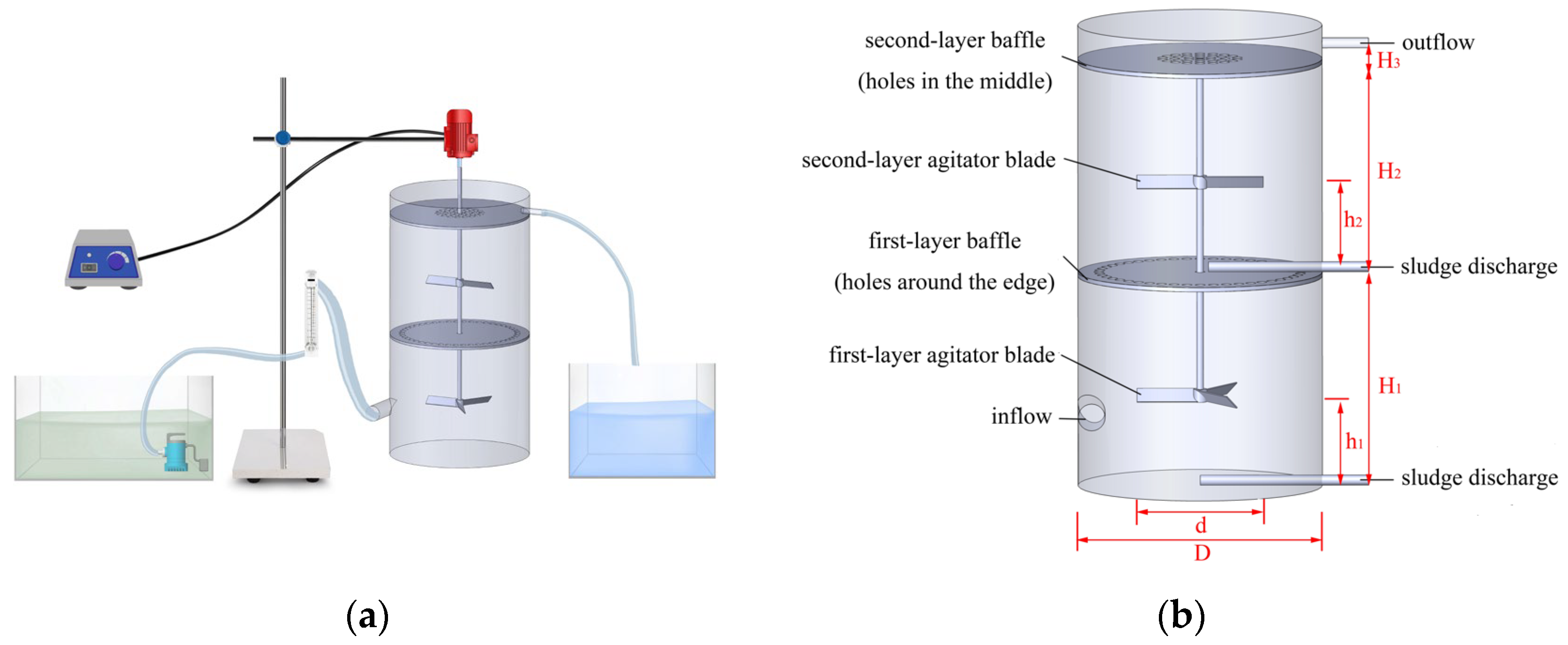
Figure 2.
Particle diameter distribution diagram of simulated wastewater.
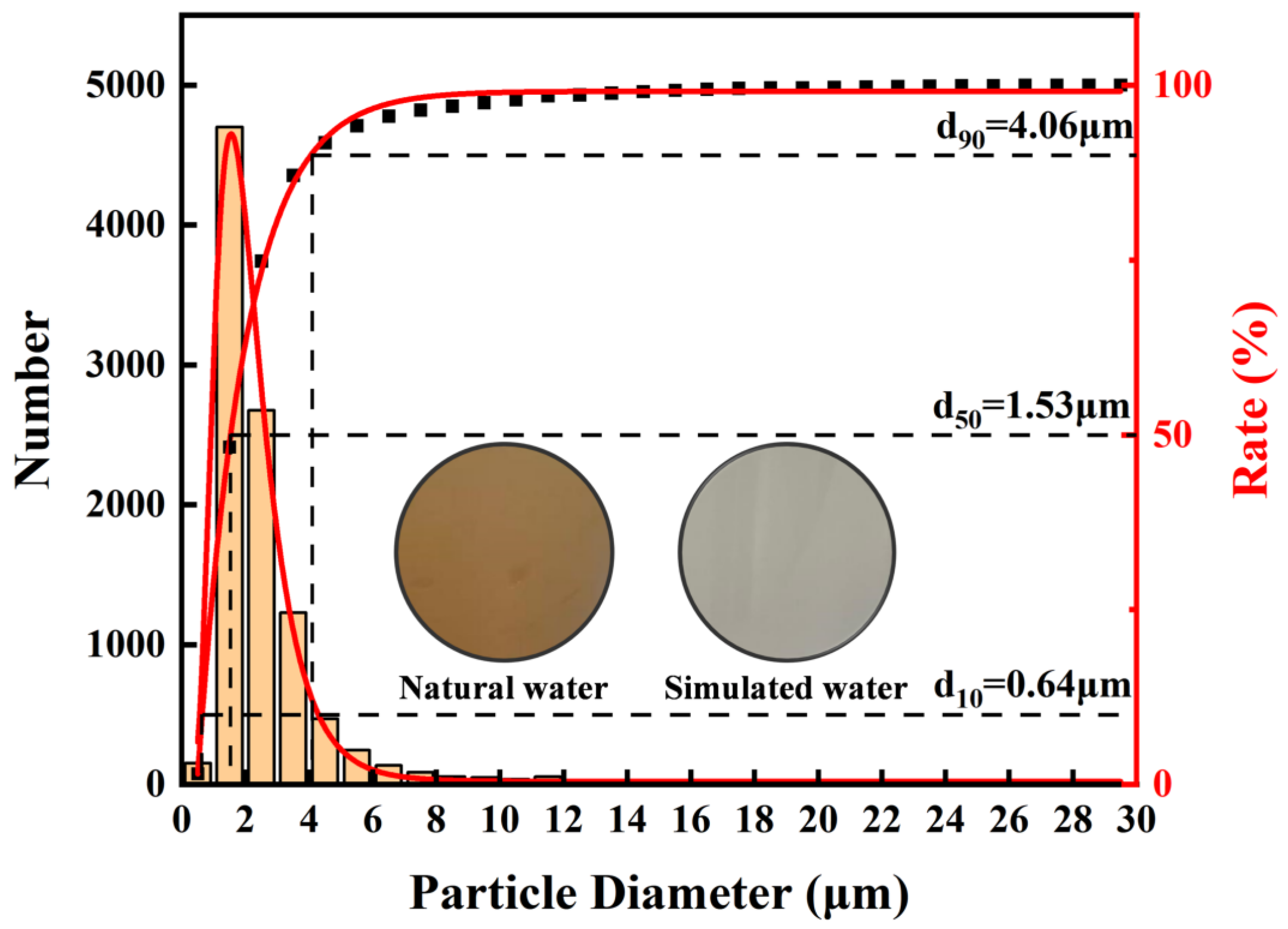
Figure 3.
Mesh independence verification and mesh partitioning diagram. (a) Mesh independence verification diagram; (b) Model diagram; (c) Overall mesh partitioning diagram; (d) Mesh partitioning cross-section diagram; (e) Local mesh partitioning diagram.
Figure 3.
Mesh independence verification and mesh partitioning diagram. (a) Mesh independence verification diagram; (b) Model diagram; (c) Overall mesh partitioning diagram; (d) Mesh partitioning cross-section diagram; (e) Local mesh partitioning diagram.
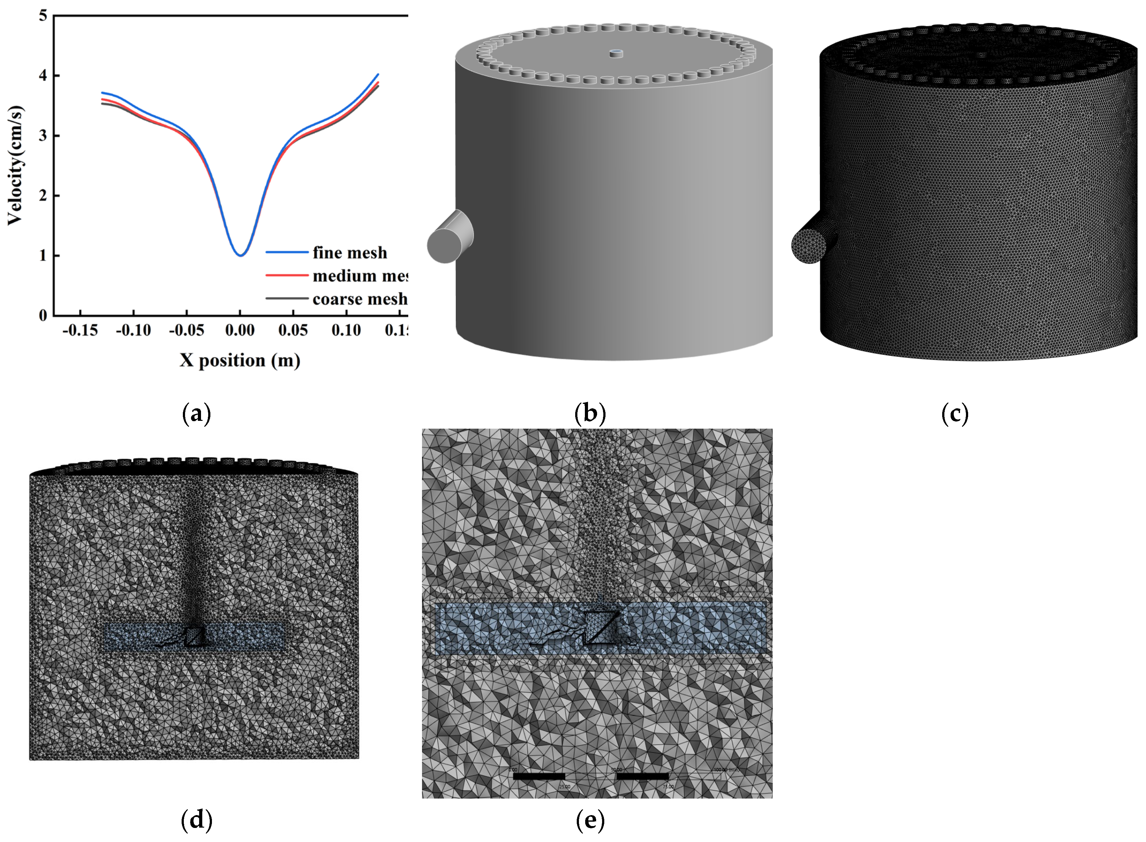
Figure 4.
Total sediment removal efficiency under different operating conditions. (a) Experimental results at agitator speeds of 10–50 rpm; (b) Experimental results with 1–4 agitator blades; (c) Experimental results at agitator heights of 60–100 mm; (d) Vortex diagram beneath the agitator blades. (Simulated water concentration = 200 mg/L, HRT = 5 min, agitator speed = 10–50 rpm, agitator blade number = 1–4 blades, agitator height = 60–100 mm).
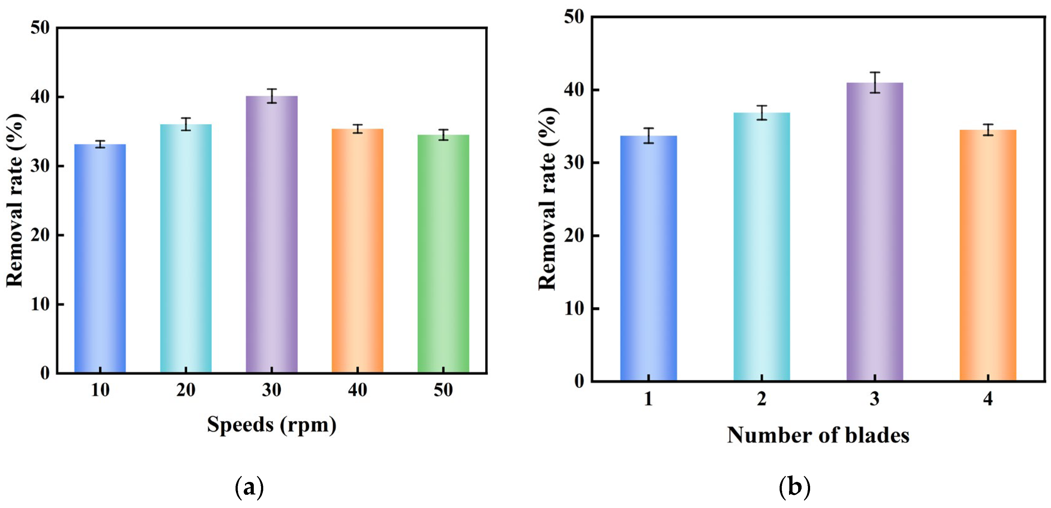
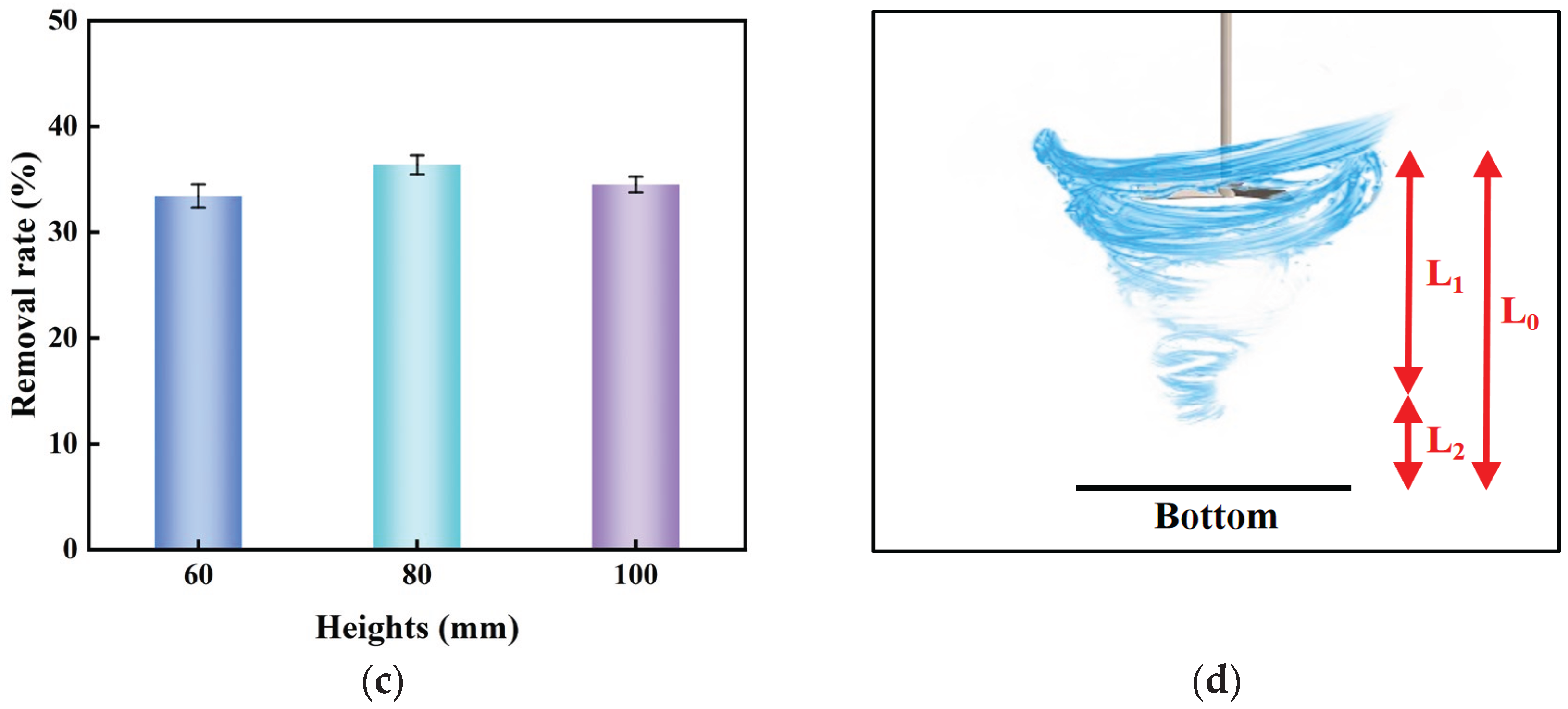
Figure 5.
Removal efficiency of different sediment particles under various operating conditions. (a) Experimental results at agitator speeds of 10–50 rpm; (b) Experimental results with 1–4 agitator blades; (c) Experimental results at agitator heights of 60-100 mm. (Simulated water concentration = 200 mg/L, HRT = 5 min, agitator speed = 10–50 rpm, agitator blade number = 1–4 blades, agitator height = 60–100 mm).
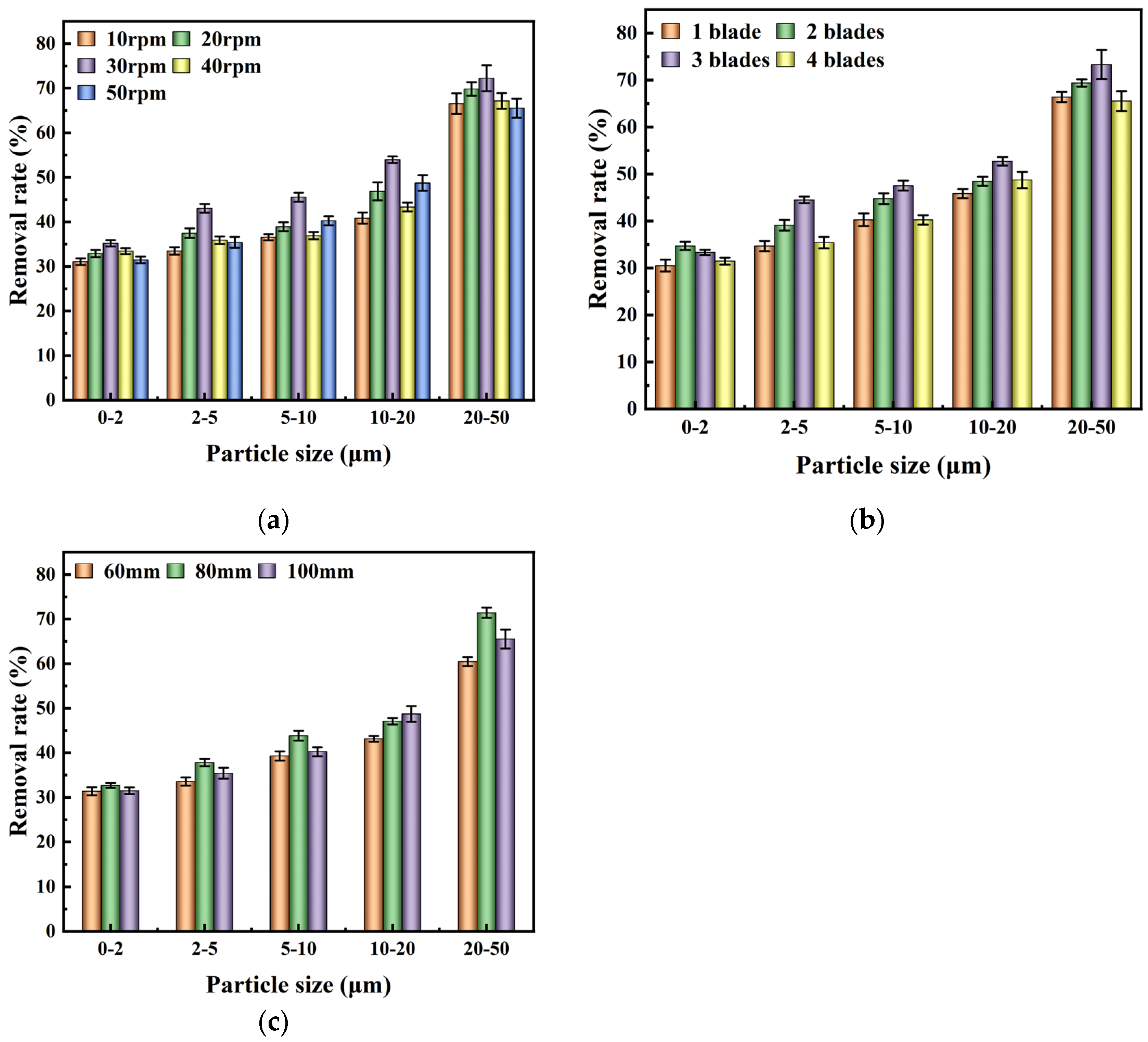
Figure 6.
TKE contour plots at different agitator speeds. (a) Speed = 50 rpm; (b) Speed = 40 rpm; (c) Speed = 30 rpm; (d) Speed = 20 rpm; (e) Speed = 10 rpm. (Simulated water concentration = 200 mg/L, HRT = 5 min, agitator blade number = 4, agitator height = 100 mm).
Figure 6.
TKE contour plots at different agitator speeds. (a) Speed = 50 rpm; (b) Speed = 40 rpm; (c) Speed = 30 rpm; (d) Speed = 20 rpm; (e) Speed = 10 rpm. (Simulated water concentration = 200 mg/L, HRT = 5 min, agitator blade number = 4, agitator height = 100 mm).
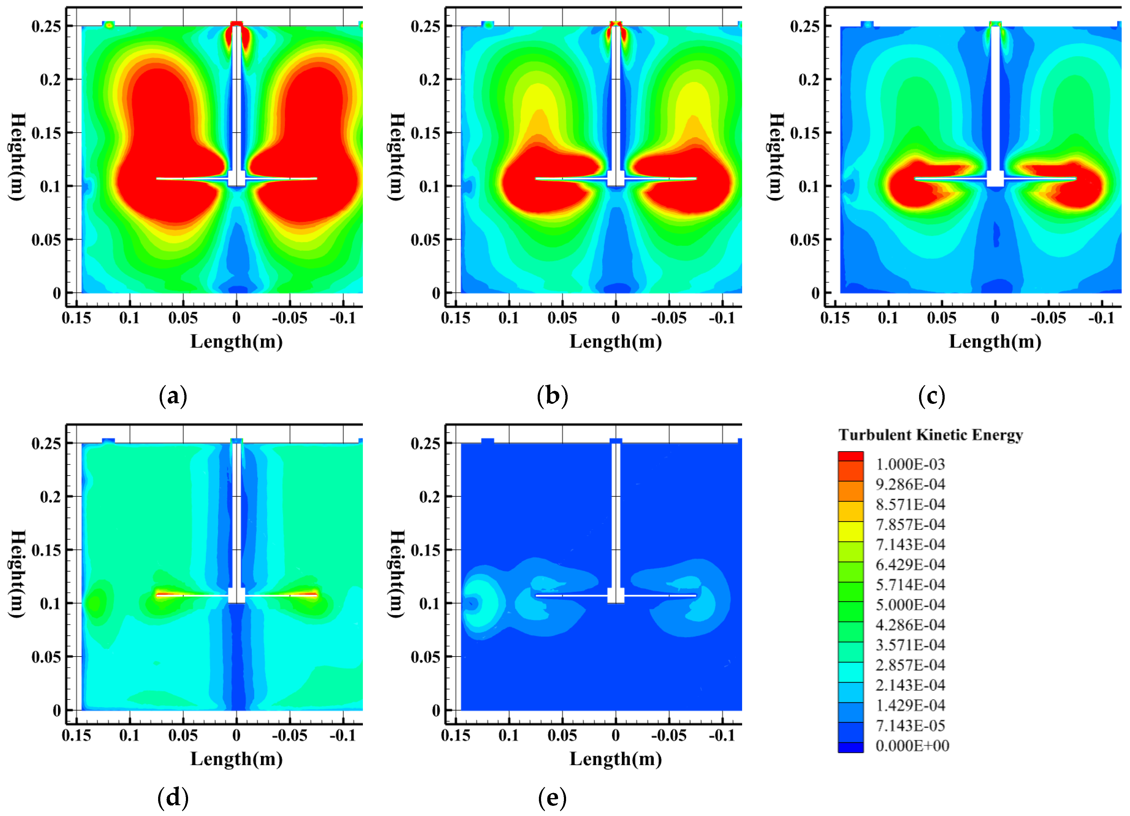
Figure 7.
Velocity streamlines at different agitator speeds. (a) Speed = 50 rpm; (b) Speed = 40 rpm; (c) Speed = 30 rpm; (d) Speed = 20 rpm; (e) Speed = 10 rpm. (Simulated water concentration = 200 mg/L, HRT = 5 min, agitator blade number = 4, agitator height = 100 mm).
Figure 7.
Velocity streamlines at different agitator speeds. (a) Speed = 50 rpm; (b) Speed = 40 rpm; (c) Speed = 30 rpm; (d) Speed = 20 rpm; (e) Speed = 10 rpm. (Simulated water concentration = 200 mg/L, HRT = 5 min, agitator blade number = 4, agitator height = 100 mm).
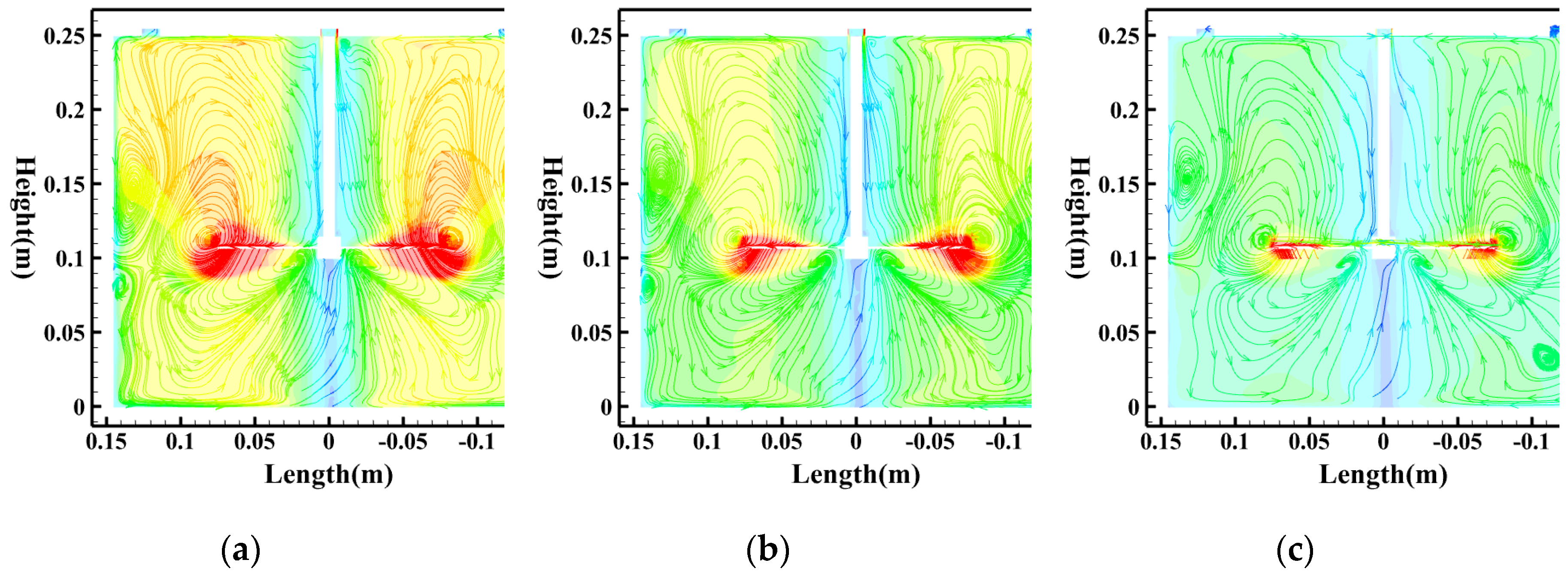
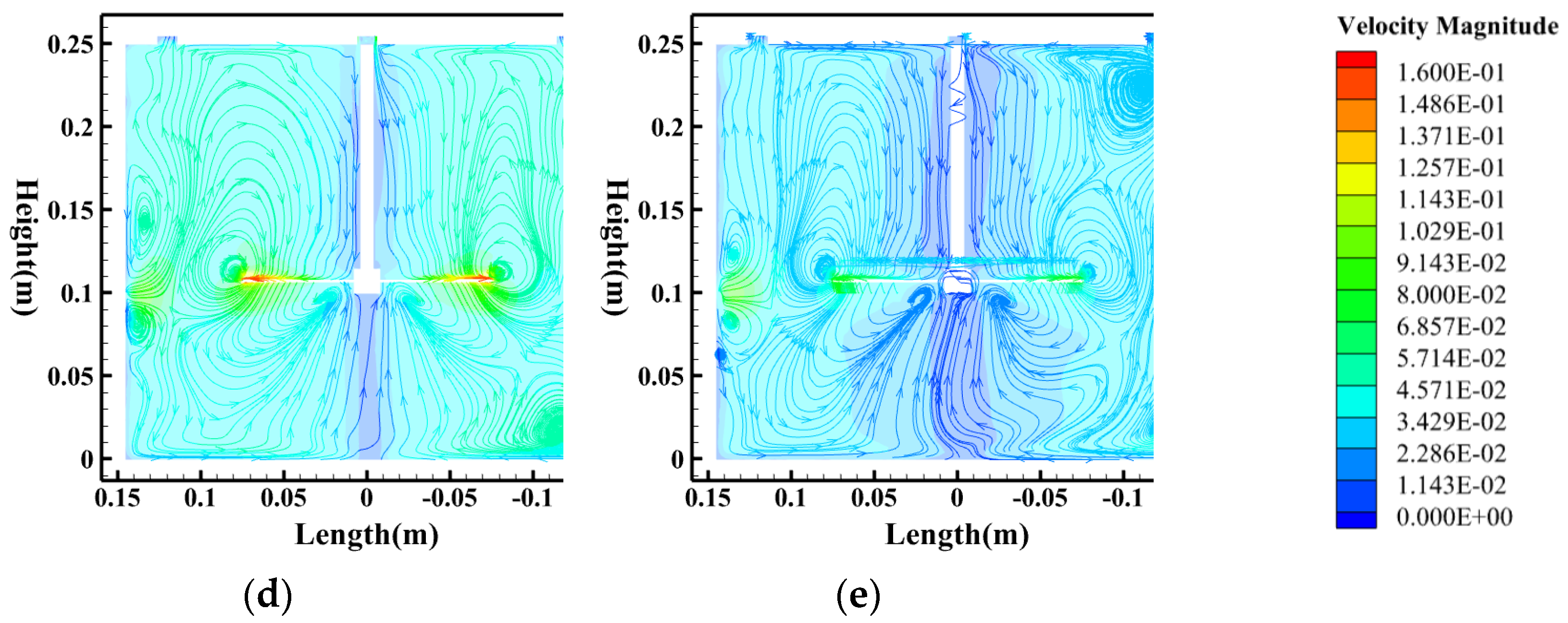
Figure 8.
TKE contour plots at different agitator blade numbers. (a) Four blades; (b) Three blades; (c) Two blades; (d) One blade. (Simulated water concentration = 200 mg/L, HRT = 5 min, agitator speed = 50 rpm, agitator height = 100 mm).
Figure 8.
TKE contour plots at different agitator blade numbers. (a) Four blades; (b) Three blades; (c) Two blades; (d) One blade. (Simulated water concentration = 200 mg/L, HRT = 5 min, agitator speed = 50 rpm, agitator height = 100 mm).
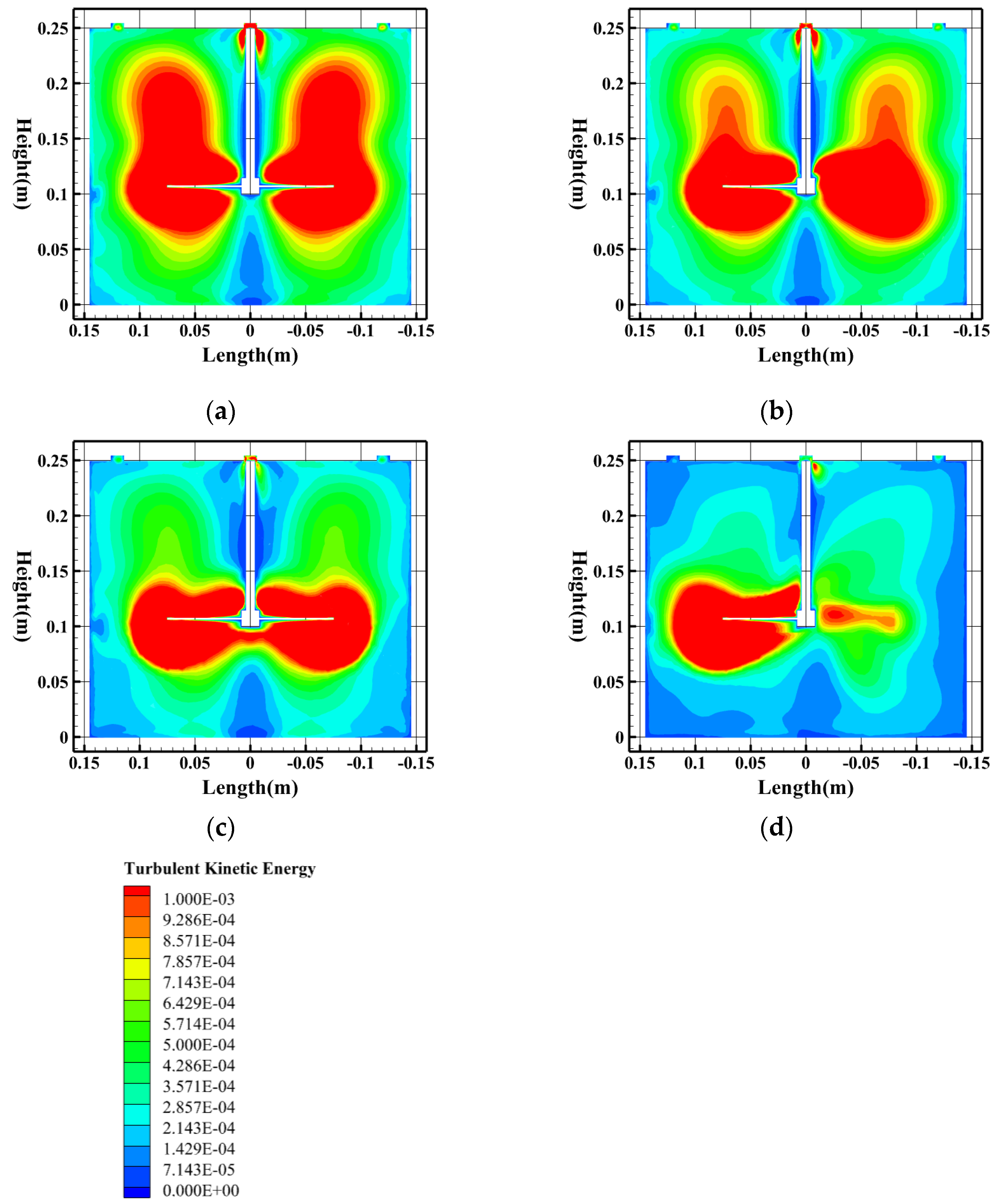
Figure 9.
Velocity streamlines at different agitator blade numbers. (a) Four blades; (b) Three blades; (c) Two blades; (d) One blade. (Simulated water concentration = 200 mg/L, HRT = 5 min, agitator speed = 50 rpm, agitator height = 100 mm).
Figure 9.
Velocity streamlines at different agitator blade numbers. (a) Four blades; (b) Three blades; (c) Two blades; (d) One blade. (Simulated water concentration = 200 mg/L, HRT = 5 min, agitator speed = 50 rpm, agitator height = 100 mm).
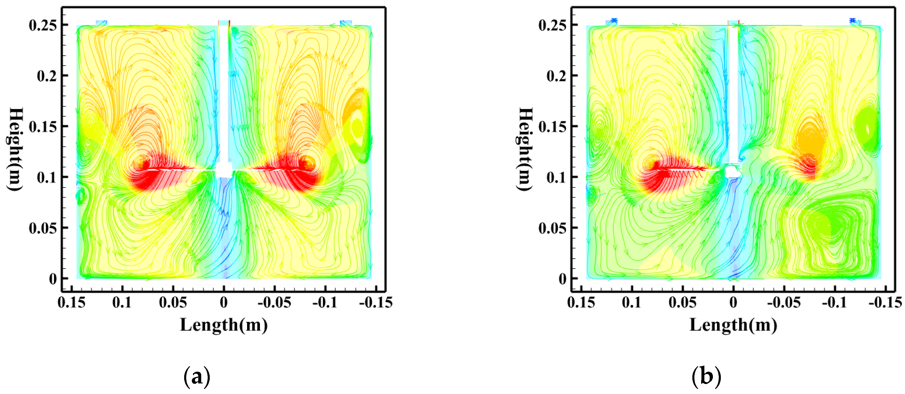
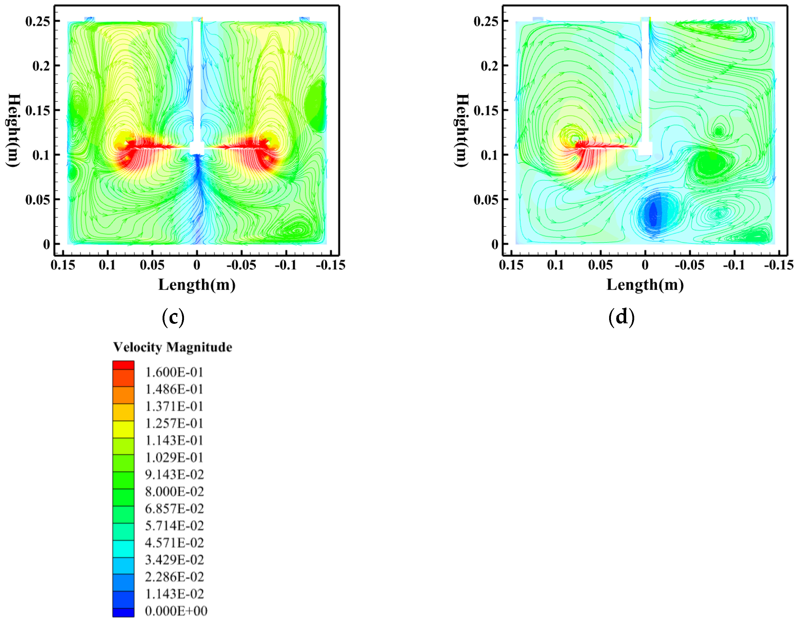
Figure 10.
TKE contour plots at different agitator heights. (a) Agitator height = 100 mm; (b) Agitator height = 80 mm; (c) Agitator height = 60 mm. (Simulated water concentration = 200 mg/L, HRT = 5 min, agitator speed = 50 rpm, agitator blade number = 4).
Figure 10.
TKE contour plots at different agitator heights. (a) Agitator height = 100 mm; (b) Agitator height = 80 mm; (c) Agitator height = 60 mm. (Simulated water concentration = 200 mg/L, HRT = 5 min, agitator speed = 50 rpm, agitator blade number = 4).
Figure 11.
Velocity streamlines at different agitator heights. (a) Agitator height: 100 mm; (b) Agitator height: 80 mm; (c) Agitator height: 60 mm. (Simulated water concentration = 200 mg/L, HRT = 5 min, agitator speed = 50rpm, agitator blade number = 4).
Figure 11.
Velocity streamlines at different agitator heights. (a) Agitator height: 100 mm; (b) Agitator height: 80 mm; (c) Agitator height: 60 mm. (Simulated water concentration = 200 mg/L, HRT = 5 min, agitator speed = 50rpm, agitator blade number = 4).
Figure 12.
Schematic of particle flocculation process.
Figure 13.
Flocculant dosage concentration experiment. (a) Floc images at PAC dosages ranging from 20 mg/L to 160 mg/L; (b) Floc images at PAM dosages ranging from 0.5 mg/L to 2.0 mg/L; (c) Turbidity variation at PAC dosages ranging from 20 mg/L to 160 mg/L; (d) Turbidity variation at PAM dosages ranging from 0.5 mg/L to 2.0 mg/L. (Simulated water concentration = 200 mg/L, HRT = 10 min, agitator speed = 50 rpm).
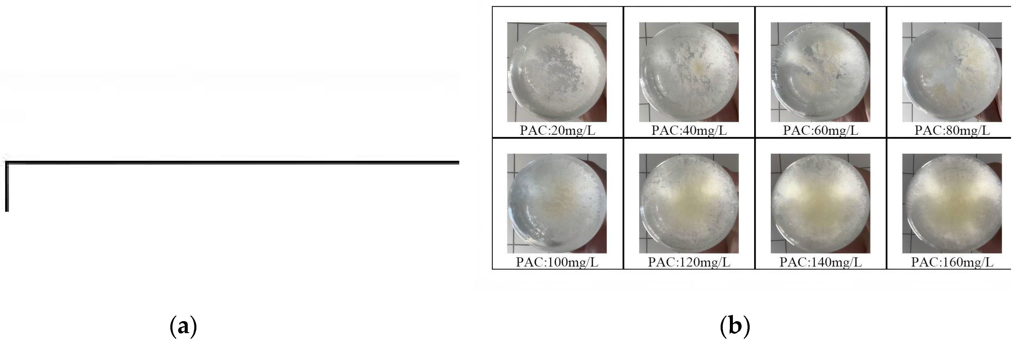
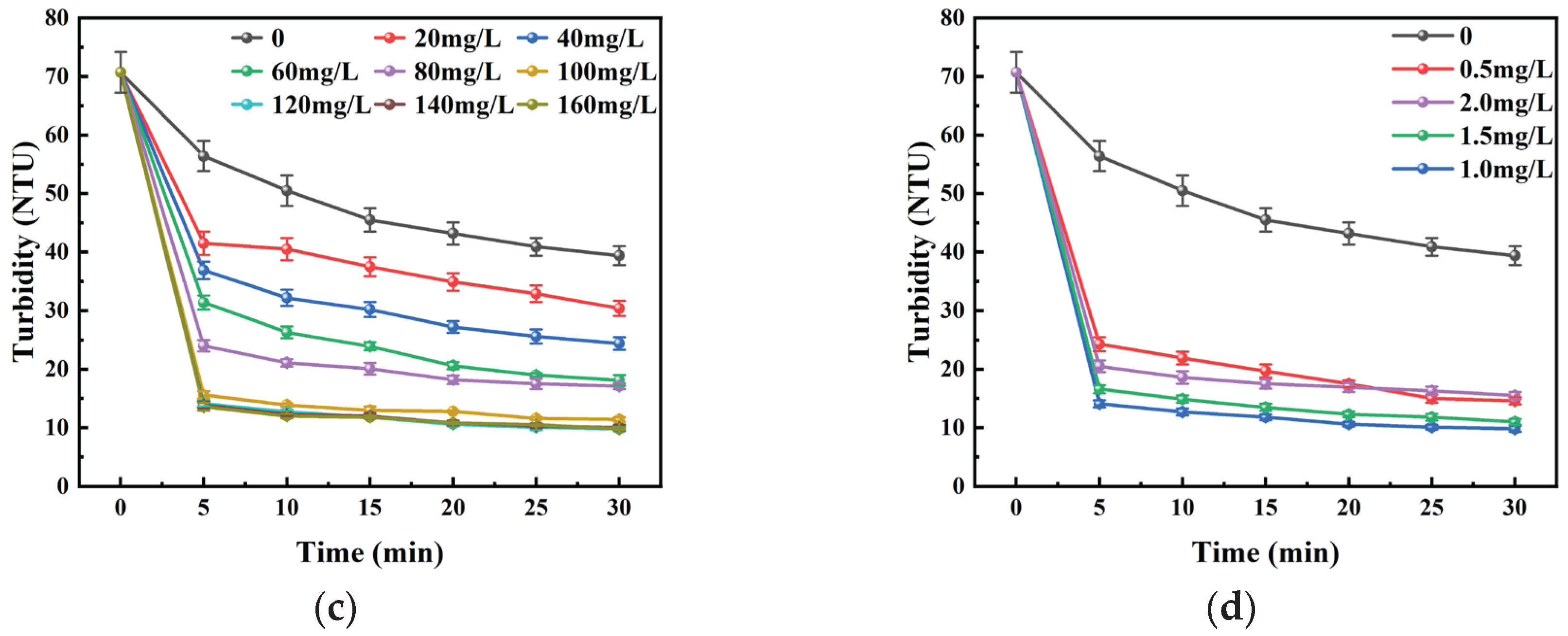
Figure 14.
Comparison of turbidity effects from different factors in the second layer. (a) Experimental results for agitator blade number 1–4; (b) Experimental results for agitator height 60–100 mm. (Simulated feed concentration = 200 mg/L, HRT = 10 min, agitator speed = 30 rpm).
Figure 14.
Comparison of turbidity effects from different factors in the second layer. (a) Experimental results for agitator blade number 1–4; (b) Experimental results for agitator height 60–100 mm. (Simulated feed concentration = 200 mg/L, HRT = 10 min, agitator speed = 30 rpm).
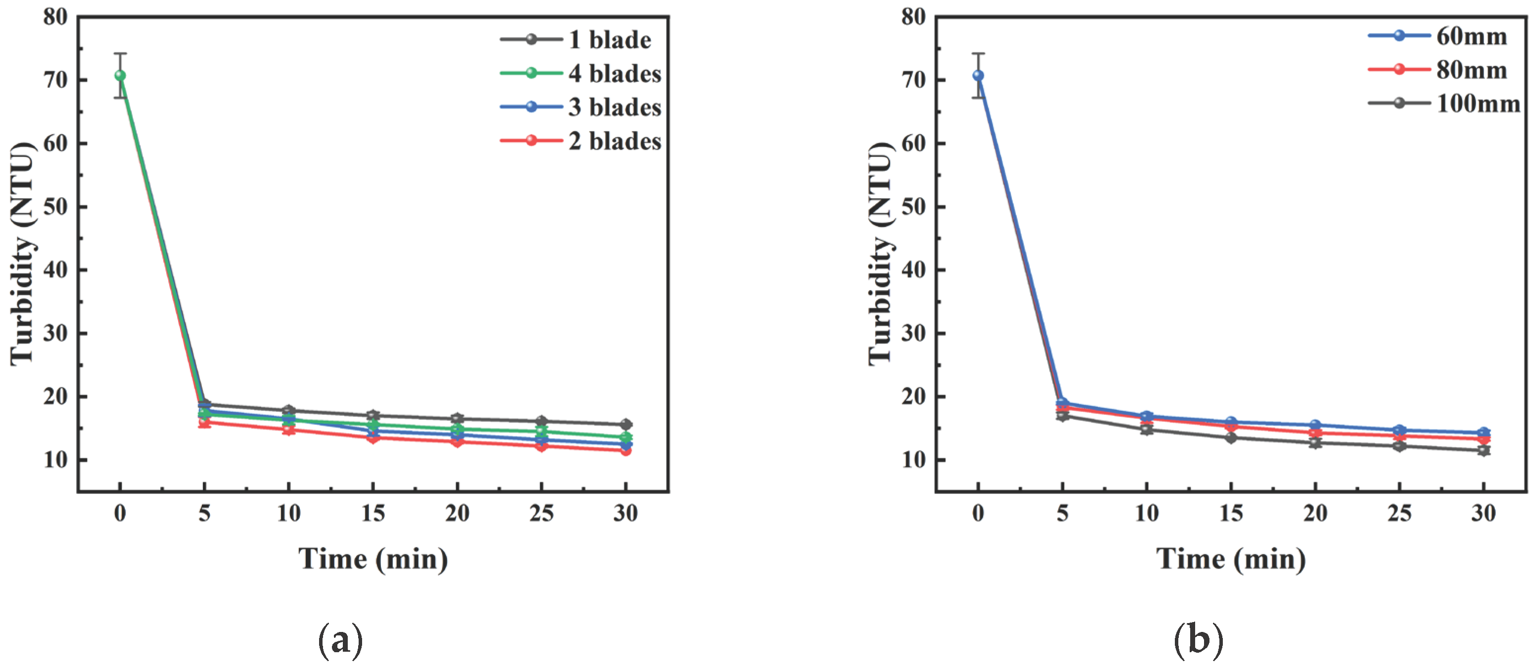

Table 1.
Major instruments.
| Instrument name | Instrument model | Manufacturer |
|---|---|---|
| Forced-air drying oven | DHG-9023A | Shanghai Hecheng Instrument Manufacturing Co., Ltd. |
| Digital microscope | EX33 | Ningbo Shunyu Instrument Co., Ltd. |
| Reduced-speed variable-frequency electric stirrer | GE-1T | Changzhou Yuexin Instrument Manufacturing Co., Ltd. |
| Magnetic stirrer | M-SCL | Hangzhou Qiwei Instrument Co., Ltd. |
| Oil-free vacuum Pump | HL-15L | Zhongshan Ruihai Electromechanical Equipment Co., Ltd. |
| Measuring and controlling instrument | BPM-AHGB1V0N | Beijing Yuanchang Testing Technology Co., Ltd |
Table 2.
Multi-layer separation tank dimensions.
| Parameter | H1 (mm) | H2 (mm) | H3 (mm) | h1 (mm) | h2 (mm) | D (mm) | d (mm) |
|---|---|---|---|---|---|---|---|
| value | 250 | 250 | 50 | 60-100 | 60-100 | 300 | 150 |
Table 3.
Water sample particle diameter distribution.
| Sample | Turbidity | Concentration | Particle diameter | ||||
|---|---|---|---|---|---|---|---|
| <2µm | 2–5µm | 5–10µm | 10–20µm | >20µm | |||
| Raw water | 67.8 NTU | 193.4 mg/L | 45.27% | 42.51% | 6.98% | 3.80% | 1.44% |
| Simulated water | 70.7 NTU | 200.0 mg/L | 48.21% | 42.43% | 5.73% | 2.14% | 1.49% |
Table 4.
Water sample particle diameter distribution.
| Particle diameter | <2µm | 2–5µm | 5–10µm | 10–20µm | >20µm |
|---|---|---|---|---|---|
| Turbidity | 34.64% | 45.80% | 50.58% | 56.14% | 75.25% |
Table 5.
Comparison of experimental and predicted values for a specific operating condition.
| Operating condition | Particle diameter (μm) | Average particle diameter (μm) |
Experimental Value (%) | Predicted value(%) | Absolute error(%) | ||
|---|---|---|---|---|---|---|---|
| Agitator speed (rpm) |
Agitator blade number (pieces) | Agitator height (mm) | |||||
| 50 | 4 | 100 | 0–2 | 1.44 | 31.46 | 30.61 | 0.85 |
| 2–5 | 2.92 | 35.42 | 33.33 | 2.09 | |||
| 5–10 | 6.65 | 40.26 | 39.76 | 0.50 | |||
| 10–20 | 13.31 | 48.73 | 49.81 | 1.08 | |||
| 20–50 | 27.91 | 65.55 | 66.07 | 0.52 | |||
Table 6.
Average error analysis table for all operating conditions.
| Operating condition | Average Absolute Error (%) | ||
|---|---|---|---|
| Agitator speed (rpm) |
Agitator blade number (pieces) | Agitator height (mm) | |
| 50 | 4 | 100 | 1.01 |
| 40 | 4 | 100 | 2.74 |
| 30 | 4 | 100 | 0.95 |
| 20 | 4 | 100 | 2.43 |
| 10 | 4 | 100 | 3.34 |
| 50 | 3 | 100 | 3.98 |
| 50 | 2 | 100 | 3.01 |
| 50 | 1 | 100 | 2.75 |
| 50 | 4 | 80 | 2.41 |
| 50 | 4 | 60 | 2.83 |
Table 7.
Comparison of turbidity between two processes.
| Process 1 | Turbidity (NTU) | ||||
|---|---|---|---|---|---|
| 5min | 10min | 15min | 20min | 25min | |
| Multi-layer separation + sedimentation | 16.2 | 15.0 | 13.1 | 12.2 | 11.0 |
| Traditional flocculation + sedimentation | 25.8 | 21.0 | 18.4 | 16.3 | 14.5 |
1 Operating parameters of the multi-layer separation tank: The agitator speed is 30 rpm, with the agitator height for the first-layer being 80 mm and the agitator height for the second-layer being 100 mm. The number of agitator blades for the first-layer is 3, and the number of agitator blades for the second layer is 2.
Disclaimer/Publisher’s Note: The statements, opinions and data contained in all publications are solely those of the individual author(s) and contributor(s) and not of MDPI and/or the editor(s). MDPI and/or the editor(s) disclaim responsibility for any injury to people or property resulting from any ideas, methods, instructions or products referred to in the content. |
© 2026 by the authors. Licensee MDPI, Basel, Switzerland. This article is an open access article distributed under the terms and conditions of the Creative Commons Attribution (CC BY) license (http://creativecommons.org/licenses/by/4.0/).
Copyright: This open access article is published under a Creative Commons CC BY 4.0 license, which permit the free download, distribution, and reuse, provided that the author and preprint are cited in any reuse.


