Submitted:
08 February 2026
Posted:
09 February 2026
You are already at the latest version
Abstract
A new, efficient algorithm for generating monitoring spreadsheets for the optical coating production with monochromatic layer thickness monitoring is presented. Due to its high computational efficiency, it has no limit on the number of different wavelengths used to monitor different groups of deposited coating layers. The algorithm allows for the use of various criteria to select the optimal sequence of monitoring wavelengths. Several examples are provided demonstrating the application of the algorithm to various types of multilayer filters.
Keywords:
thin films
; optical coatings
; monochromatic monitoring
; monitoring spreadsheet
1. Introduction
Monochromatic monitoring has been used to produce optical coatings with non-quarter-wave optical thicknesses for over forty years. In its original form, called level monitoring [1,2], it provides signals to terminate layer deposition upon reaching specified monitoring signal termination levels. These levels are pre-calculated based on known thicknesses of a theoretical coating design. Unfortunately, accurate control of layer thicknesses using level monitoring is difficult, since “small errors in early layers affect the shape of the [monitoring] curve for later layers” (Angus Macleod, ([3], p. 506)]. To overcome, or at least minimize, this negative effect, modern monochromatic monitoring equipment uses active corrections of termination levels based on information about the actual monitoring signal, primarily on the extreme values of this signal recorded during the coating deposition [4,5,6].
In the context of monitoring with correction of termination levels, the concept of monitoring signal swing is very useful ([7], pp.194-196). In particular, the formula for correction of termination levels follows directly from the consideration of this concept [7]. It is also important for creating monitoring spreadsheets, the correct specification of which allows for the full utilization of all the advantages of modern monitoring equipment.
In the case of direct monochromatic monitoring, when all layers are monitored on one of the produced samples, the monitoring spreadsheet is a table in which each layer is assigned a specific monitoring wavelength and a signal termination level. This table may also contain sets of other parameters important for accurate layer thickness control. For many years, the creation of monitoring spreadsheets depended almost entirely on the practical experience of the optical coatings engineer. Early attempts to automate this procedure [8,9] were not oriented towards the use of monitoring with termination level correction. Automated procedures that take into account specific requirements for reliable monitoring with termination level correction were proposed in [10,11].
This paper proposes a new computationally efficient algorithm for creating monitoring spreadsheets for coatings with large numbers of layers and virtually unlimited number of monitoring wavelength switches between groups of layers, with each of these groups being monitored at an optimally selected monitoring wavelength. A description of the algorithm is given in Section 2. Examples of the application of this algorithm with requirements similar to those considered in [11] are given in Section 3. Conclusions are presented in Section 4.
2. Algorithm for Creating a Monitoring Spreadsheet
This section discusses the algorithm for direct monitoring in transmission mode, but it can also be used for monitoring in reflection mode and for creating monitoring spreadsheets for witness chips, if a strategy with multiple monitoring chips is used [6]. As in [10,11], the selection of monitoring wavelengths for the coating layers is based on several criteria specified for the dependence of monitoring signal (transmittance) on the deposited layer thickness. As an example, we will use the criteria discussed in [11] as the most important ones. These are the criteria specified for the start amplitude of the monitoring signal and for its swing value at the beginning and end of layer deposition. It will be seen that the main part of the algorithm is independent of the set of selected criteria, and the algorithm can be directly used for any other combination of the criteria discussed in [10,11].
In [11], the start amplitude of the monitoring signal is the difference between the transmittance level at the beginning of layer deposition (the initial level) and the first transmittance extremum during the layer deposition. Since this difference can be either positive or negative, we will consider its absolute value and denote it as value (see Figure 1). This quantity will be called entry variation. The extremum of the monitoring signal is not necessarily reached during the layer deposition, and we will extend the definition of the entry variation for such situations. If there is no signal extremum during the layer deposition, then is equal to the absolute value of the difference between the transmittance initial level and the termination level (the transmittance level at the end of layer deposition).
Along with the value, we will consider the initial and final swing values, and . By definition, is related to the termination level, by the formula:
Here and are the last two monitoring signal extrema recorded during layer deposition. The values included in this formula are shown in Figure 1. The value is calculated similarly to the value, but the equation uses the initial level instead of .
We assume that the transmittance is measured as a percentage. Consequently, is also measured as a percentage. The same applies to the and . Figure 1 shows that their values are close to 0% or 100% if the initial or termination levels are close to the maximum or minimum values of the monitoring signal.
Figure 1 illustrates the monitoring of a relatively thick layer, for which two monitoring signal extrema are reached during the deposition process. However, extending the concept of initial and final swing values to thinner layers, when only one or even no extremes are reached, presents no problem. The expected monitoring signal is pre-calculated using the well-known analytical formulas [7], and in these formulas we can extend the deposition time to the left from the start of the layer deposition. This allows calculating the virtual last and previous monitoring extrema [12].
As noted in the introduction, the use of monochromatic monitoring with termination level correction requires the creation of monitoring spreadsheets with specific requirements to the monitoring signal behavior. Such requirements are particularly important for the monitoring signal at the beginning and end of layer deposition [10,11]. As an example, we will use the requirements that are considered most important in [11]. We require that the entry variation EV exceeds a%, and that the initial and final swing values be within the specified limits. The specific values of a and swing limits in percentage will be set in Section 3.
To take these requirements into account, we introduce three partial penalty functions, for
for
and for similarly to the Equation (3).
The penalty function f is the sum of these partial penalty functions:
Note that the penalty functions is zero if all requirements are met. The parameters and in Equations (2) and (3) will be specified in Section 3.
Let be the number of coating layers, and be the number of wavelength points in the wavelength grid used to select monitoring wavelengths. When creating a monitoring spreadsheet, our goal is to assign to each coating layer a monitoring wavelength at which the deposition of this layer should be monitored. The penalty function introduced above depends on the number of the design layer and the number of the monitoring wavelength in the specified wavelength grid ( varies from 1 to ). Therefore, we will denote as the penalty function value for the -th layer monitored at -th wavelength. In the algorithm under consideration, the selection of monitoring wavelengths is based on minimizing the penalty function values . Furthermore, the algorithm also takes into account the requirement to limit the number of wavelength switches during coating deposition. This means that the algorithm generates a specified number of groups of successive design layers, with each group monitored at its own monitoring wavelength. This is shown schematically in Figure 2.
The algorithm begins by generating a matrix with the elements specified above. This is an by matrix, where is typically significantly larger than . The next step is to generate an by matrix the elements of which are
When choosing the optimal monitoring wavelength for a sequence of layers, starting with layer and ending with layer , we consider the sums of penalty functions for all these layers at different monitoring wavelengths. It is natural to choose the monitoring wavelength so that this sum is minimal. It is easy to see that these sums are equal to the differences . We denote the minimum of this sum by :
and the monitoring wavelength at which this minimum is achieved by .
We now introduce the table with elements defined by Eq. (6). Note that this is an by table. Since , we only specify its elements on and above the main diagonal. Along with the minimum values defined by Eq. (6), this table also stores the wavelengths at which the minima are reached. This table is the key element of our algorithm. It allows us to select the optimal layer sequences and the optimal monitoring wavelengths for these sequences for any given number of wavelength switches during coating deposition.
In the extreme case where the monitoring wavelength is the same for all coating layers, the optimal monitoring wavelength is the one listed along with in the upper right corner of the table. If one or more wavelength switches are set, the optimal combinations are also easily found from this table. Because the table has small dimensions, all calculations are fast. In all the examples discussed in the next section, the calculations take fractions of a second on a typical laptop.
3. Examples of Application of the Algorithm
In all examples of this section, we set the following requirements for , and values. We require that and both swing values be between 10% and 90%. The parameters and in Equations (2) and (3) are equal to 4 and 0.2, respectively. We consider three filters with significantly different structures. In all three cases, the monitoring wavelengths are selected in the spectral range from 400 to 800 nm with a wavelength step of 5 nm.
3.1. Cut Filter
In this sub-section, we consider a 36-layer cut filter similar to that considered in [5]. As in [5], the layer materials are TiO2 and SiO2, and the substrate is BK7 glass. The first layer from the substrate is a high index layer. The theoretical transmittance of the filter and the physical thicknesses of its layers are shown in Figure 3. The filter under consideration has 36 layers instead of 42 in [5], but its structural properties are similar to those in [5]. It has two fairly thin first layers.
When constructing the monitoring spreadsheet, we successively increase the number of monitoring wavelengths that can be used to monitor the filter. When only one monitoring wavelength is allowed for all layers, the algorithm selects 555 nm. It turns out that with this selection, the monitoring requirements (see above) are violated for six design layers: layers 1 through 4, as well as layers 34 and 36. Increasing the number of different wavelengths to 2 and then to 3 reduces the number of layers with violated requirements to 4 and 3, respectively.
Figure 4 shows the monitoring signal corresponding to three different monitoring wavelengths. The signal is highlighted in pink in the layers where monitoring requirements are violated. These are layers 2, 4, and 36.
For layer 2, and . Layer 2 is one of two thin design layers. Meeting all the requirements for such layers is often difficult. However, the algorithm selected a wavelength that best meets both requirements. For layer 4, and for layer 36, . Further increasing the number of wavelength switches does not improve these figures.
3.2. Hot Mirror
Here we consider a 44-layer hot mirror with model high and low refractive indices of its layers equal to 2.35 and 1.45, and a substrate refractive index of 1.52. The first layer from the substrate is a high index layer. The theoretical transmittance of the hot mirror and the physical thickness of its layers are shown in Figure 5.
The hot mirror has no thin layers. However, it turns out that to meet the monitoring requirements formulated at the beginning of this section, we need a relatively large number of wavelengths switches. With three different monitoring wavelengths, the monitoring requirements are violated for eight design layers, with four wavelengths, for seven layers, and only with seven different monitoring wavelengths is the number of such layers reduced to three.
Figure 6 shows the monitoring signal corresponding to seven monitoring wavelengths. The signal is highlighted in pink in the layers where monitoring requirements are violated. These are layers 24, 26, and 32.
For layer 24, , for layer 26, . and for layer 32, . Clearly, the violations of the formulated requirements should be considered minor.
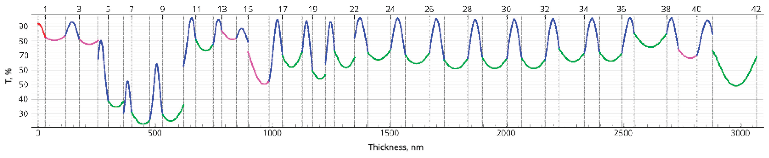
3.3. Long Pass Filter
The long pass filter discussed in this subsection has 42 layers, model high and low refractive indices of 2.35 and 1.45, and a substrate refractive index of 1.52. The first layer from the substrate is a high index layer. The theoretical transmittance of the filter and the physical thickness of its layers are shown in Figure 7.
The layers of this filter are thinner than those of the hot mirror. Therefore, one might expect that more wavelengths switches would be required to meet monitoring requirements. And this is indeed the case. With seven different monitoring wavelengths, we are left with eight layers where monitoring requirements are violated. Increasing the number of different monitoring wavelengths to eight reduces the number of such layers to five.
Figure 8 shows the monitoring signal corresponding to eight monitoring wavelengths. The signal is highlighted in pink in the layers where monitoring requirements are violated. These are layers 2, 4, 14, 16, and 40.
For layer 2, , for layer 4, , for layer 14, , for layer 16, ., and for layer 40, . Further complication of the monitoring strategy does not lead to significant improvement in the results.
4. Conclusions
A new algorithm for generating monitoring spreadsheets for the coating production with monochromatic monitoring of layer thicknesses is presented. The algorithm is based on assessing the quality of monitoring of successive groups of coating layers at a given monitoring wavelength. To assess this quality, various criteria for selecting a monitoring wavelength can be specified, and a penalty function is introduced that takes these criteria into account. The key element of the algorithm is the construction of a table that stores the minimum values of the penalty function and the optimal monitoring wavelengths for different groups of coating layers. Due to a small dimension of the introduced table, the computational efficiency of the proposed algorithm is high, and it has no limitations on the number of different wavelengths used to monitor the coating production.
The algorithm’s application is demonstrated using the examples of generating monitoring spreadsheets for three structurally different multilayer filters. In these examples, we used monitoring wavelength selection criteria that are essential for the reliable application of monochromatic monitoring procedures with on-line correction of the monitoring signal termination levels. In all examples, monitoring spreadsheets containing up to eight different monitoring wavelengths are generated in a fraction of a second on a standard laptop.
Author Contributions
Conceptualization, original draft preparation, A.V.T; Software, investigation, S.K.K.; Methodology, validation, A.A.T; Data curation, review, and editing, S.A.S. All authors have read and agreed to the published version of the manuscript.
Funding
The theoretical research underlying the development of the presented algorithm was conducted under the state assignment of Lomonosov Moscow State University.
Institutional Review Board Statement
Not applicable.
Informed Consent Statement
Not applicable.
Data Availability Statement
Data are contained within the article.
Conflicts of Interest
The authors declare no conflicts of interest.
References
- Macleod, H.A. Monitoring of optical coatings. Appl. Opt. 1981, 20, 82–89. [Google Scholar] [CrossRef] [PubMed]
- Zhao, F. Monitoring of periodic multilayers by the level method. Appl. Opt. 1985, 24, 3339–3342. [Google Scholar] [CrossRef] [PubMed]
- Macleod, H.A. Thin-Film Optical Filters, 4th ed.; CRC Press: Boca Raton, FL, USA; Taylor & Francis Group: Abingdon, UK, 2010. [Google Scholar]
- Zoeller, A.; Boss, M.; Goetzemann, R.; Hagedorn, H.; Klug, W. Substantial progress in optical monitoring by intermittent measurement technique. In Advances in Optical Thin Films II; Amra, C., Kaiser, N., Macleod, H.A., Eds.; SPIE, 2005; vol. 5963, p. 59630D. [Google Scholar]
- Zoeller, A.; Boss, M.; Hagedorn, H.; Romanov, B. Computer simulation of coating processes with monochromatic monitoring in Advances in Optical Thin Films III; SPIE, 2008; vol. 7101, pp. 188–194. [Google Scholar]
- Zöller, A.; Hagedorn, H.; Weinrich, W.; Wirth, E. Testglass changer for direct optical monitoring. Proc. SPIE 2011, 8168, 81681J. [Google Scholar]
- Tikhonravov, A. Optical Coatings: Design, Characterization, Monitoring; 2024, SPIE, 2024. [Google Scholar]
- Holm, C. Optical thin film production with continuous reoptimization of layer thicknesses. Appl. Opt. 1978, 18, 1978–1982. [Google Scholar] [CrossRef] [PubMed]
- Tikhonravov, A.V.; Trubetskov, M.K.; Amotchkina, T.V. Statistical approach to choosing a strategy of monochromatic monitoring of optical coating production. Appl. Opt. 2006, 45, 7863–7870. [Google Scholar] [CrossRef] [PubMed]
- Trubetskov, M.; Amotchkina, T.; Tikhonravov, A. Automated construction of monochromatic monitoring strategies. Appl. Opt. 2015, 54, 1900–1909. [Google Scholar] [CrossRef] [PubMed]
- Zideluns, J.; Lemarchand, F.; Arhilger, D.; Hagedorn, H.; Lumeau, J. Automated optical monitoring wavelength selection for thin film filters. Opt. Express 2021, 29, 33398–33413. [Google Scholar] [CrossRef] [PubMed]
- Kochikov, I.V.; Lagutin, Y. S.; Lagutina, A. A.; Lukyanenko, D.V.; Tikhonravov, A.V.; Yagola, A.G. Stable method for optical monitoring the deposition of multilayer optical coatings. Comput. Math. Math. Phys. 2020, 60, 2056–2063. [Google Scholar] [CrossRef]
Figure 1.
To the introduction of the entry variation EV and swing values.
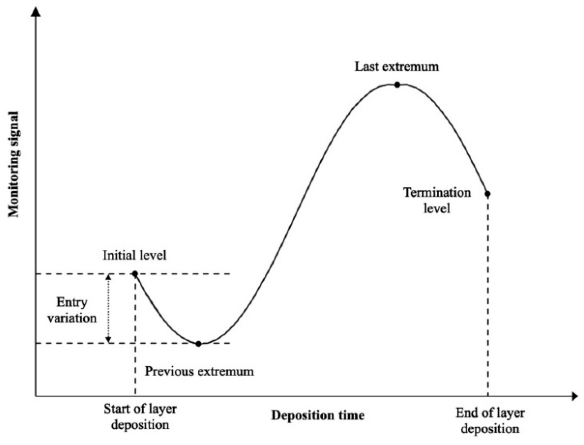
Figure 2.
Dividing the design into groups of layers, with each group monitored at its own wavelength.
Figure 2.
Dividing the design into groups of layers, with each group monitored at its own wavelength.
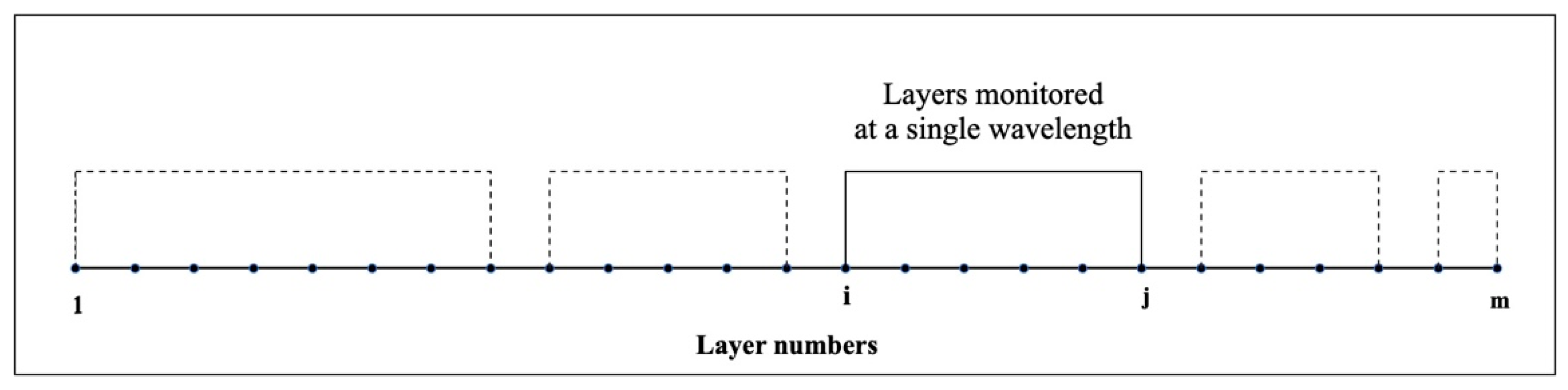
Figure 3.
(a) Theoretical transmittance (a) andlayer physical thicknesses (b) of a 36-layer cut filter.
Figure 3.
(a) Theoretical transmittance (a) andlayer physical thicknesses (b) of a 36-layer cut filter.
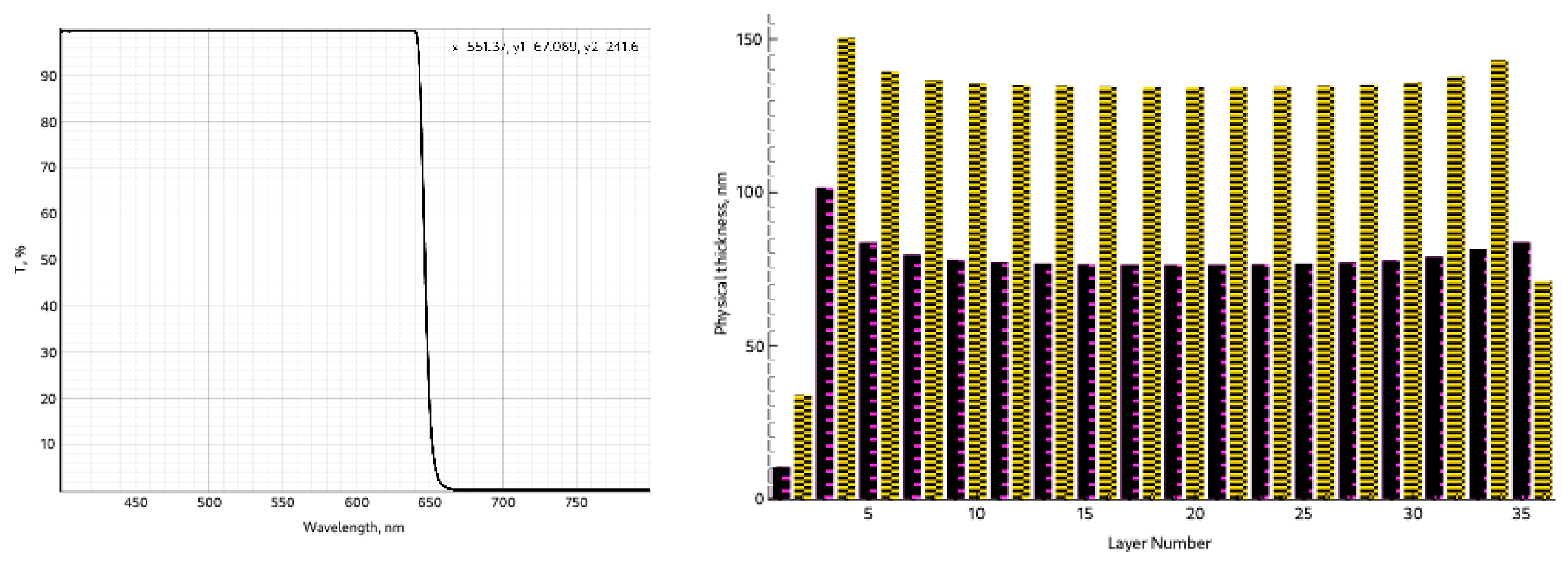
Figure 4.
Monitoring signal for a 36-layer cut filter: layers 1-3 are monitored at 400 nm, layers 4-35 at 590 nm, and layer 36 at 645 nm.
Figure 4.
Monitoring signal for a 36-layer cut filter: layers 1-3 are monitored at 400 nm, layers 4-35 at 590 nm, and layer 36 at 645 nm.
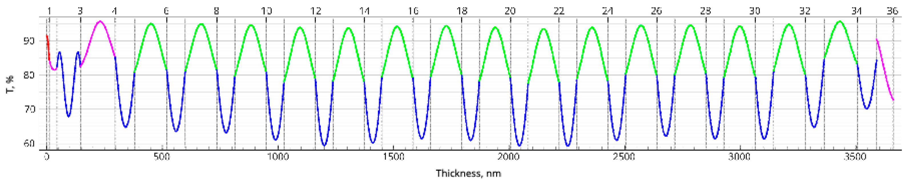
Figure 5.
Theoretical transmittance (a) and layer physical thicknesses (b) of a 44-layer hot mirror.
Figure 5.
Theoretical transmittance (a) and layer physical thicknesses (b) of a 44-layer hot mirror.
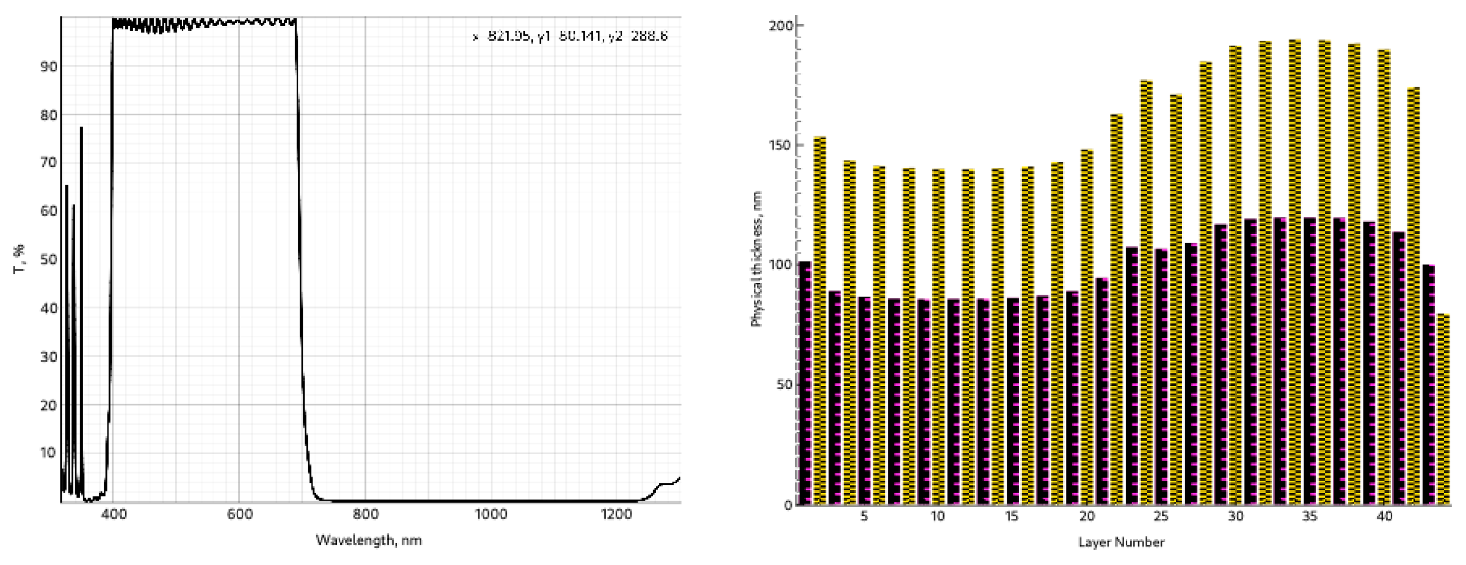
Figure 6.
Monitoring signal for a 44-layer hot mirror: layers 1-2 are monitored at 595 nm, layers 3-27 at 665 nm, layer 28 at 490 nm, layers 29-38 at 405 nm, layers 39-41 at 410 nm, layers 42-43 at 660 nm, and layer 44 at 490 nm.
Figure 6.
Monitoring signal for a 44-layer hot mirror: layers 1-2 are monitored at 595 nm, layers 3-27 at 665 nm, layer 28 at 490 nm, layers 29-38 at 405 nm, layers 39-41 at 410 nm, layers 42-43 at 660 nm, and layer 44 at 490 nm.
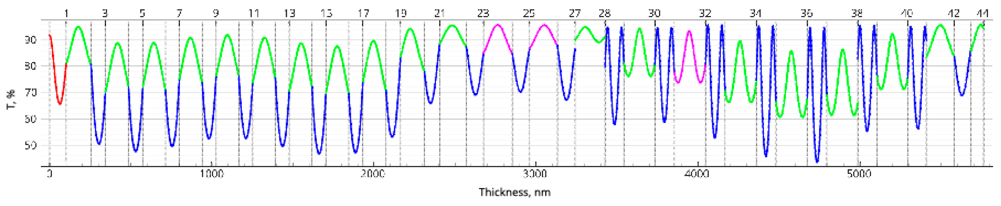
Figure 7.
Theoretical transmittance (a) and layer physical thicknesses (b) of a 42-layer long pass filter.
Figure 7.
Theoretical transmittance (a) and layer physical thicknesses (b) of a 42-layer long pass filter.
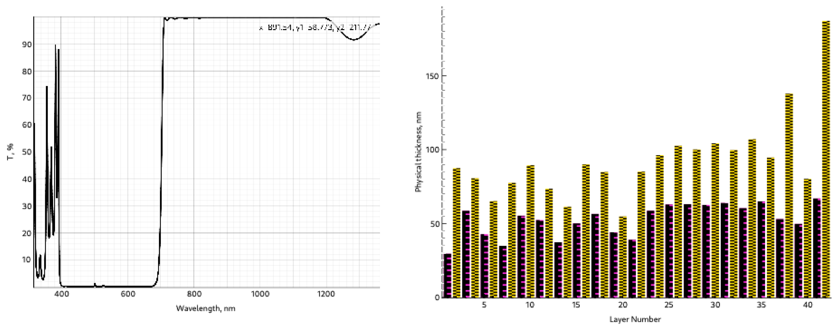
Figure 8.
Monitoring signal for a 42-layer long pass filter: layers 1-4 are monitored at 800 nm, layers 5-6 at 575 nm, layers 7-10 at 520 nm, layers 11-15 at 545 nm, layers 16-20 at 530 nm, layers 21-22 at 535 nm, layers 23-41 at 745 nm, and layer 42 at 705 nm.
Figure 8.
Monitoring signal for a 42-layer long pass filter: layers 1-4 are monitored at 800 nm, layers 5-6 at 575 nm, layers 7-10 at 520 nm, layers 11-15 at 545 nm, layers 16-20 at 530 nm, layers 21-22 at 535 nm, layers 23-41 at 745 nm, and layer 42 at 705 nm.
Disclaimer/Publisher’s Note: The statements, opinions and data contained in all publications are solely those of the individual author(s) and contributor(s) and not of MDPI and/or the editor(s). MDPI and/or the editor(s) disclaim responsibility for any injury to people or property resulting from any ideas, methods, instructions or products referred to in the content. |
© 2026 by the authors. Licensee MDPI, Basel, Switzerland. This article is an open access article distributed under the terms and conditions of the Creative Commons Attribution (CC BY) license (http://creativecommons.org/licenses/by/4.0/).
Copyright: This open access article is published under a Creative Commons CC BY 4.0 license, which permit the free download, distribution, and reuse, provided that the author and preprint are cited in any reuse.


