
Submitted:
08 February 2026
Posted:
09 February 2026
Read the latest preprint version here
Abstract
Sample-wise detection of P-, R-, and T-peaks in electrocardiograms (ECGs) is challenging because each peak type is sparsely represented (≈1:500 samples in a typical 10-s, 500-Hz ECG at 60 bpm), such that even a small number of false-positives (FPs) can markedly degrade positive predictive value (PPV) and limit the practicality of classifier-only approaches. This study proposes a lightweight ECG peak detection framework that combines binary classifiers with a physiological temporal constraints (PTC) algorithm to address extreme sample-level class imbalance. Local morphological features are first evaluated using lightweight machine-learning models, among which XGBoost (XGB) exhibited the most stable score-ranking performance. Rather than directly thresholding classifier outputs, prediction scores are interpreted through PTCs that encode physiological timing relationships. R-peaks are detected using score ranking combined with a refractory-period constraint, and the detected R-peaks serve as temporal landmarks for subsequent P- and T-peak detection within physiologically plausible time windows reflecting the P–QRS–T sequence. Quantitative evaluation was conducted using the Lobachevsky University Electrocardiography Database, hereafter referred to as LUDB. With a temporal tolerance of ±20 ms, the XGB-based system achieved an F1-score of 0.87 for R-peak detection (sensitivity 0.96, PPV 0.79), corresponding to approximately 9–10 true R-peaks with only 2–3 FP samples per 10-s segment. For P- and T-peaks, F1-scores of 0.70 and 0.69 were obtained, respectively. Additional evaluation on arrhythmic LUDB records and qualitative application to ECG recordings from the PTB-XL database demonstrated physiologically consistent behavior. These results indicate that reliable and interpretable ECG peak detection under extreme class imbalance can be achieved by integrating lightweight classifiers with explicit PTC algorithms, without reliance on complex deep learning architectures.
Keywords:
ECG
; peak detection
; extreme class imbalance
; false-positive reduction
; physiological temporal constraints
; binary classifier
1. Introduction
Accurate detection of P, R, and T-peaks in electrocardiograms (ECGs) is a fundamental task for a wide range of clinical and research applications, including heart rate variability analysis, arrhythmia diagnosis, pharmacological evaluation, and long-term physiological monitoring. Numerous automatic peak detection algorithms have been proposed, ranging from classical methods based on differentiation [1,2,3], integration, and thresholding—such as the Pan–Tompkins algorithm—to more recent data-driven approaches.
In recent years, machine learning and deep learning techniques have been increasingly applied to ECG analysis, including peak detection and waveform interpretation [4,5,6]. In particular, convolutional neural network (CNN)-based methods that directly process waveform segments, as well as deep models that exploit long-range temporal context, have demonstrated high performance in tasks such as ECG waveform delineation and segmentation, where the onset and offset of P, QRS, and T waves are estimated as temporal intervals [4,5,6,7,8,9,10,11]. Although these approaches often allow peak locations to be inferred from the estimated waveform structures, relatively few studies explicitly address ECG peak detection as a primary objective, especially for low-amplitude P and T-peaks. However, many deep learning approaches require large amounts of annotated training data and involve complex model architectures with high computational cost. In addition, their internal decision-making processes are often opaque, making it difficult to interpret detection results, analyze failure cases, or manually adjust parameters when false-positives (FPs) occur.
In practical operating environments, ECG recordings frequently contain baseline drift, noise, and various types of arrhythmia, and reliable ground-truth annotations are not always available. Under such conditions, practical usability, interpretability, and FP suppression are often more important than marginal improvements in classification accuracy. This is particularly true for applications involving long-term recordings, large-scale datasets, or interactive graphical user interfaces (GUIs) that allow manual peak correction, where low computational complexity and transparent algorithmic behavior are essential.
One of the main challenges in ECG peak detection is that P and T-peaks generally exhibit much lower amplitudes than R-peaks and often have ambiguous local morphologies. When low-amplitude peaks are evaluated solely based on local waveform shape, reliable discrimination between P and T-peaks becomes difficult. In contrast, human ECG interpretation typically relies on a stable temporal structure: P peaks precede R-peaks, and T-peaks follow R-peaks. Thus, once an R-peak is identified as a temporal landmark, the recognition of neighboring P and T-peaks becomes substantially easier.
Although ECG interpretation strategies vary among observers, a common cognitive process involves first identifying the most salient and high-amplitude QRS complex—particularly the R-peak—and then recognizing P and T-peaks in relation to this landmark based on their temporal order. In this study, we explicitly incorporate this human-inspired interpretation process into the algorithmic design by modeling the physiological temporal order of ECG components as physiological temporal constraints (PTC).
When applying machine learning to ECG peak detection, extreme class imbalance presents an additional challenge. For example, in a 10-s ECG segment sampled at 500 Hz, assuming a heart rate of 60 bpm, only a small fraction of samples (approximately 10 samples per peak type) correspond to a given P-, R-, or T-peak, while the vast majority (approximately 4990 samples per task) represent background. Under such conditions, indiscriminately increasing the number of features may cause the classifier to learn noise or spurious correlations, leading to degraded generalization performance and excessive FPs. Because performance measures that are dominated by true-negative counts—such as overall classification rate and specificity—tend to take artificially high values under extreme class imbalance, they become largely uninformative in this setting. This problem becomes more severe at higher sampling frequencies, where the number of background samples increases while the number of true peaks remains unchanged.
Although unsupervised learning approaches such as clustering or anomaly detection have been explored for imbalanced data, ECG peak identification is fundamentally defined by clinically established criteria. Ignoring annotated peak labels may therefore result in detections that conflict with clinical interpretation. Accordingly, this study adopts a supervised learning framework using medically defined peak labels and combines the resulting prediction scores with PTC-based interpretation.
Rather than aiming to maximize peak detection performance using deep learning models, this study focuses on a lightweight and interpretable design that explicitly targets sample-wise peak detection. Simple binary classifiers are used to estimate prediction scores that reflect local peak likelihood at the individual-sample level based on waveform morphology. The primary role of the classifier is to provide a coarse probabilistic indication of local, sample-wise peak likelihood. The main contributions of this study are summarized as follows:
(a) explicit incorporation of human-inspired ECG interpretation into algorithm design via physiological temporal constraints (PTC);
(b) realization of stepwise sample-wise P-, R-, and T-peak detection using R-peaks as temporal landmarks, effectively reducing FPs through the combination of lightweight classifiers and PTC;
(c) demonstration of practical applicability through quantitative evaluation on the Lobachevsky University Electrocardiography Database (LUDB) and qualitative visualization using PTB-XL, a large publicly available electrocardiography dataset.
2. Methods
2.1. Dataset
This study used the LUDB [12,13,14]. LUDB provides 12-lead ECG recordings with beat-level annotations of P waves, QRS complexes, and T waves assigned by experienced cardiologists.
A total of 142 recordings diagnosed as sinus rhythm (SR) were analyzed (male: 49 ± 18 years, n = 77; female: 55 ± 19 years, n = 65). Among the 12 leads, only leads II, V5, and V6 were used, because the morphologies of P waves, QRS complexes, and T waves were relatively clearly observable in these leads. Thus, three leads were analyzed per subject, resulting in a data length of 3 × 10 s × 500 Hz = 15,000 samples per subject.
Each recording was segmented into 10-s time windows. For each sample point, cardiologist-provided annotations were used to determine whether it corresponded to a P-peak, R-peak, or T-peak. Labels were encoded as integer values (P = 1, R = 2, T = 3), and all remaining samples were treated as non-peak (background).
To prevent information leakage between subjects, the data were randomly divided at the record level into training (80%), tuning (10%), and test (10%) sets. This subject-wise split was repeated ten times, and classifier training and evaluation were performed independently for each split. The results for each split were saved in separate output directories.
2.2. Signal Preprocessing
For feature extraction, a sliding window centered at each sample point was employed. The window length was specified directly in the number of samples as
Because the sampling frequency was 500 Hz, these window lengths correspond to 14, 18, 22, 26, and 30 ms, respectively.
Prior to feature extraction, the ECG signals were filtered using a low-pass filter (LPF) with a cutoff frequency of 40 Hz (CFL= 40Hz) to suppress high-frequency noise and spike-like artifacts while preserving the morphological characteristics of the P, QRS, and T waves. The half-window length was defined as
At the signal boundaries, complete windows could not be formed; therefore, samples within ±half points from the edges were excluded from the analysis.
2.3. Feature Extraction
For each central sample , a symmetric local window
was extracted from the ECG signal, and 11 lightweight morphological features were computed. These features were designed to capture local waveform characteristics common to P, R, and T waves while keeping the computational cost low.
(a) Amplitude and statistical features
First, statistical features describing the amplitude distribution within the window and the relative prominence of the center sample were defined as
where wleft and wright denote the left and right sub windows divided at the center sample.
These features represent the local amplitude level, left–right asymmetry, and the prominence of the center point.
(b) Differential and curvature features
To characterize the local slope and curvature around the center sample, first- and second-order difference features were defined as
These correspond to the first-order central difference (local slope) and the discrete second-order difference (local curvature), respectively, and help distinguish the sharp morphology of the QRS complex from the smoother P and T waves.
(c) Slope and energy-based features
To capture the global trend and local variability within the window, the following two features were introduced.
where denotes the sample index within the window, and and are their respective mean values. The feature f7 represents the slope of the linear regression fitted to the windowed waveform, reflecting its overall increasing or decreasing trend.
where is the window length. This feature corresponds to the difference energy, defined as the mean squared first-order difference, and reflects the local roughness or high-frequency content of the waveform.
(d) Direct amplitude information
Finally, direct amplitude-related features were included as
These features provide absolute amplitude information at the center sample and within the window, complementing the relative and differential descriptors.
These features serve as local morphological descriptors that are commonly applicable to P-, R-, and T-peaks and are computationally efficient, making them suitable for high-speed processing. For each waveform type, a binary classification problem was formulated by treating samples with the corresponding label as positive and all other samples as negative.
2.4. Classification Models
Independent binary classifiers were constructed for the detection of P-, R-, and T-peaks. In this study, six machine learning methods with different characteristics, ranging from linear to nonlinear models, were evaluated for comparison.
(a) XGBoost (XGB)
XGB is a decision-tree ensemble method based on gradient boosting. The following hyperparameters were tuned:
Class imbalance was addressed using the scale_pos_weight parameter.
(b) Logistic Regression (LGR)
LGR is a linear classification model with L2 regularization. The regularization parameter
was used as a tuning parameter. Features were standardized prior to training, and class imbalance was handled using class_weight = “balanced”.
(c) Quadratic Discriminant Analysis (QDA)
QDA is a discriminant analysis method that assumes class-specific covariance matrices. In this study, the standard implementation was used without additional hyperparameter tuning.
(d) Naive Bayes (NB)
Gaussian NB was employed. This method assumes conditional independence among features and that each feature follows a normal distribution. Default parameter settings were used without hyperparameter tuning.
(e) k-Nearest Neighbors (KNN)
KNN is a nonparametric method that performs classification based on distances in feature space. Euclidean distance was used as the distance metric, and the number of neighbors was treated as a tuning parameter:
Features were standardized to account for the influence of scale on distance calculations.
(f) Linear Discriminant Analysis (LDA)
LDA is a linear classifier that assumes multivariate normal distributions for each class and maximizes the ratio of between-class variance to within-class variance. In this study, the standard LDA formulation with a shared covariance matrix across classes was used, without additional hyperparameter tuning.
Each classifier outputs a posterior probability indicating the likelihood that a given sample corresponds to a peak. In this study, this probability was referred to as the prediction score. These prediction scores were not used directly for final peak decisions but were interpreted in combination with the PTCs algorithm described in the next section.
2.5. Peak Detection Algorithm Based on PTC
2.5.1. Algorithm Overview
This section describes the overall structure of the peak detection algorithm designed to reduce FPs. The proposed algorithm is characterized by a stepwise processing framework that combines probabilistic peak estimation using machine learning with PTC and a cognitively inspired design.
The algorithm is composed of the following three core components:
(a) a design aligned with the temporal structure of ECG signals and the human cognitive process of ECG interpretation,
(b) suppression of FP R-peaks through score-based descending-order processing combined with a refractory period constraint,
(c) reduction of the search space for P- and T-peaks using R-peaks as temporal landmarks based on PTCs.
By applying these components sequentially, the proposed method suppresses erroneous detections that are difficult to avoid using machine learning alone and achieves practical and interpretable peak detection performance.
Generation and Score-Based Ordering of R-Peak Candidates
First, the trained R-peak classifier was applied to all sample points of the ECG signal, and the probability that each time index corresponded to an R-peak was calculated as an R-peak prediction score.
The resulting prediction scores and their corresponding time indices were stored as a two-dimensional array and sorted in descending order of the prediction score. This procedure established an ordered list in which R-peak candidates could be evaluated sequentially, starting from the most likely candidate.
By explicitly defining the order in which candidates are accepted or rejected, this score-based ordering clarifies the decision process and enables efficient application of subsequent temporal constraints.
R-Peak Candidate Selection Using a Refractory Period
Around the QRS complex, multiple adjacent samples often exhibit high R-peak prediction scores for a single heartbeat. Consequently, simple threshold-based detection tends to produce multiple detections of the same R-peak, resulting in FPs.
To address this issue, a sequential candidate selection strategy was adopted that combines probability thresholding with a refractory period. Candidate R-peaks are processed in descending order of prediction score, and a candidate is rejected if its temporal distance from an already selected R-peak falls within the refractory period. The concept of a refractory period is motivated by the suppression of multiple detections introduced in the Pan–Tompkins algorithm. In the Pan–Tompkins method, a refractory period of 200 ms is imposed after QRS detection to prevent re-detection within the same cardiac cycle, based on the assumption of a physiological ventricular refractory period [2].
In the present study, considering that R-peak candidates are prefiltered with high accuracy by a machine-learning classifier, the refractory period was optimized via grid search within the range of 30–80 ms. This range was chosen based on the typical temporal width of the QRS complex in adult ECGs, which is generally on the order of several tens of milliseconds to approximately 100 ms [15,16,17], as well as the sampling frequency used in this study (500 Hz, corresponding to a temporal resolution of 2 ms). Refractory periods shorter than 30 ms were insufficient to suppress multiple detections within a single QRS complex, whereas values exceeding 80 ms increased the risk of suppressing closely spaced beats, particularly under tachycardic conditions.
Through this sequential selection process, exactly one R-peak is selected per heartbeat, achieving a balance between effective suppression of multiple detections and robustness to heart rate variability.
Visualization of the Sequential Selection Process Using a Table
Table 1 presents an example of the sequential selection process for R-peak candidates.
At each step, candidate time points and their corresponding scores, sorted in descending order, are evaluated, and a decision of adoption or rejection is made based on the minimum temporal distance from previously selected R-peaks.
(i) The first candidate, which has the highest score, is unconditionally adopted.
(ii) Subsequent candidates are adopted as new beats only if they are sufficiently separated from already selected R-peaks.
(iii) Candidates located within the refractory period are rejected, even if they have high scores.
This table provides an intuitive illustration that the proposed R-peak selection is a decision-making process based on both probabilistic scores and temporal constraints.
R-Peak– Landmarked P- and T-Peak Detection
The timing of the selected R-peaks serves as a temporal landmark for each cardiac cycle. Because the ECG waveform follows a well-defined physiological sequence (P→QRS→ T), this structure was explicitly exploited in the proposed method. Specifically, for each detected R-peak, P-peak candidates were searched within a temporal window preceding the R-peak, whereas T-peak candidates were searched within a temporal window following the R-peak. Within each window, candidates were evaluated based on the output scores of the corresponding classifier, and the final peak position was determined by considering both probabilistic confidence and morphological plausibility.
By introducing R-peak–centered temporal constraints, the search space is substantially reduced, which effectively suppresses false detections of P and T waves. This strategy reflects the temporal cognitive process used by human experts when interpreting ECGs, in which P and T waves are identified after recognizing the R-peak as a reference point.
From a clinical electrophysiological perspective, the durations of major ECG intervals in adults are well established. The normal QRS duration is typically 60–100 ms, and values exceeding 120 ms are generally considered abnormal, reflecting prolonged ventricular depolarization [16,17]. The P wave precedes the QRS complex, with its initial deflection occurring approximately 120–200 ms before QRS onset, corresponding to the physiological PR interval [16,17]. In contrast, the QT interval, which encompasses ventricular depolarization and repolarization, typically spans several hundred milliseconds, with heart rate–corrected values generally considered normal up to approximately 400–460 ms [16,17].
These established temporal relationships provided a physiological basis for the design of the search windows in the proposed algorithm. P-peak detection was restricted to a temporal window covering the physiological range of the PR interval preceding the R-peak, while T-peak detection was limited to a window encompassing the expected range of the QT interval following the R-peak. This design ensures that candidate peaks are evaluated only within physiologically plausible regions, thereby reducing the likelihood of false detections caused by irrelevant waveform components or noise. In this study, P-peaks were searched approximately 40–260 ms before the R-peak, and T-peaks were searched approximately 40–450 ms after the R-peak.
Figure 1 shows the flowchart of the peak detection algorithm used in this study. In PTC algorithm, probabilistic thresholds and temporal constraints are applied sequentially to the prediction scores output by the machine-learning model. A key feature of the proposed method is that the selection of prediction scores and the application of physiological constraints are performed before generating the final peak position flags, and are tightly integrated with the machine-learning model itself. Thus, the PTC–based processing employed in this study should not be regarded as a simple post-processing step, but rather as a core component of the peak detection algorithm. In this section, we focus on the conceptual structure of the algorithm and the overall processing flow. The mathematical definitions, parameter settings, and optimization procedures based on grid search are described in detail in the following sections (Section 2.5.2, Section 2.5.3 and Section 2.5.4).
The ECG signal is first processed by a trained machine-learning classifier to generate a time series of feature-based prediction scores. These scores are then input to the PTC algorithm, where R-peaks are detected first and subsequently used as temporal landmarks for P- and T-peak detection.
2.5.2. R-Peak Detection and Parameter Tuning
The trained R-peak classifier was applied to every sample of the filtered ECG, yielding a prediction score defined as
Samples exceeding the threshold were retained as R-peak candidates:
Because multiple adjacent samples often produce high scores around a single QRS complex, a refractory period constraint was imposed. After selecting the highest-scoring candidate, all remaining candidates within the refractory window around the selected R-peak were removed:
This procedure was repeated until no candidates remained, ensuring that only one R-peak was selected per QRS complex.
A grid search was performed on the tuning set for each split. The evaluated parameters included the feature-extraction window length,
the probability threshold,
and the refractory period
For each parameter combination, the numbers of true positive (TP), FP, and false negative (FN) were aggregated across the tuning set, and the following performance metrics were computed:
The performance metrics were defined as sensitivity (Se), positive predictive value (PPV), and F1-score (F1). The parameter set yielding the highest F1 was selected as the optimal configuration for that split.
2.5.3. P-Peak Detection Within R-Centered Windows
For each detected R-peak at index , P-peak candidates were searched only within a physiologically plausible pre-R interval:
[r−Ppre, r−Ppost], Ppre > Ppost > 0
For each candidate index , the classifier produced a prediction score defined as
The most likely P-peak position was determined as
Because the prediction score function may yield high values at both local maxima and minima of the ECG waveform, a five-point local extremum constraint was additionally applied to the selected candidate to ensure physiologically plausible peak detection:
x(i−1) −x(i−2) >0, x(i) −x(i−1) ≥0, x(i+1) −x(i) ≤0, x(i+2) −x(i+1) <0
The candidate was finally accepted if
A grid search was conducted over the following parameter ranges:
Ppre ∊ { 160, 180, 200, 220, 240, 260} ms
Ppost ∊ { 40, 60, 80, 100} ms
θp ∊ { 0.05, 0.10, 0.15, 0.20, 0.25, 0.30, 0.40, 0.50, 0.60, 0.70, 0.80, 0.90, 1.00 }
The optimal combination was selected separately for each split.
2.5.4. T-Peak Detection
T-peak candidates were searched within a post-R interval defined as
[r + Tpre, r + Tpost], Tpre < Tpost
For each candidate index i, the classifier produced a prediction score defined as
The most likely T-peak position was determined as
For the same reason as in P-peak detection, the prediction score function may yield high values at both local maxima and minima of the ECG waveform. Therefore, the same five-point local extremum constraint was applied to T-peak candidates before thresholding. The candidate was accepted if
A grid search was conducted over the following parameter ranges:
Tpre ∊ {40, 60, 80, 100, 120} ms
Tpost ∊ {250, 300, 350, 400, 450} ms
θT ∊ {0.05, 0.10, 0.15, 0.20, 0.25, 0.30, 0.40, 0.50, 0.60, 0.70, 0.80, 0.90, 1.00}
The optimal parameter combination was selected separately for each split.
2.6. Evaluation Protocol
2.6.1. Baseline Classification Performance Evaluation (Without PTC)
Before incorporating PTCs, the baseline classification performance of each machine-learning classifier was evaluated. In this evaluation, the objective was to quantify the intrinsic discriminative capability of each classifier based solely on features extracted from the ECG waveform, without introducing any temporal or physiological assumptions.
Receiver operating characteristic (ROC) curves and precision–recall (PR) curves were constructed from the continuous prediction scores output by each classifier. The area under the ROC curve (AUC) was calculated from the ROC curves, while the average precision (AP) was derived from the PR curves. These metrics were employed to comprehensively assess classification performance, particularly under class-imbalanced conditions.
This baseline evaluation serves as a reference performance for quantitatively assessing the effect of the temporal constraint algorithm applied in subsequent stages.
2.6.2. Final Peak Detection Performance Evaluation (with PTC)
The peak detection performance of the final system incorporating the PTC algorithm was evaluated. In this system, probabilistic scores output by machine-learning classifiers are processed through a series of temporal constraints, including a refractory period for R-peak detection and R-peak–centered temporal search windows for subsequent P- and T-peak detection, to determine the final peak locations.
The proposed algorithm follows a pipeline structure in which R-peak detection and subsequent P- and T-peak detection are sequentially coupled, with different probability thresholds and temporal constraints applied at each stage. As a result, the final output is not a continuous prediction score but a discrete sequence of detected peaks. Owing to this structural characteristic, performance evaluation methods that assume continuous threshold variation, such as ROC or PR curves, are not applicable to the final algorithm.
For the final performance evaluation, the detected R-, P-, and T-peak timings were compared with physician-annotated reference labels. A detected peak was classified as a TP if it occurred within ±10, ±20, or ±30 ms of the reference peak; otherwise, it was classified as a FP or FN. Se, PPV, and F1 were computed across all test records and all leads for each data split. The final results are reported as the mean ± standard deviation obtained from 10-fold cross-validation.
Performance evaluation was conducted for the following temporal tolerance windows:
In this study, the ±20 ms condition was adopted as the primary evaluation criterion.
2.6.3. Handling of True Negatives (TNs) in Evaluation
In the proposed framework, TNs are not explicitly counted. This is because the algorithm is not designed to perform exhaustive sample-wise classification over all background samples. Instead, a limited set of candidate points is first identified based on classifier score ranking, and only these candidates are evaluated through a sequential, candidate-driven decision process. Samples that are not selected as candidates are excluded from the decision process and are neither classified nor counted as negative samples.
2.7. Summary of Parameter Statistics
For each data split, a single set of time-constraint parameters was obtained for R-peak, P-peak, and T-peak detection. Consequently, ten values were collected for each parameter. For these values, the median, mode, and range (min–max) were calculated to evaluate the stability and variability of the optimal parameter selection. In addition, the optimal classifier parameters for XGB, LGR, and KNN were evaluated in the same manner.
2.8. Application to Arrhythmic Data in the LUDB
Using the classifier that achieved the highest performance in the evaluation on SR data, together with its trained model and optimal parameter settings, peak detection was performed on the arrhythmic data included in the LUDB, and the detection accuracy was evaluated. The arrhythmic dataset consisted of 38 male subjects (53 ± 21 years) and 20 female subjects (52 ± 21 years).
The purpose of this analysis was to examine whether the proposed algorithm, optimized using SR data, can function properly under arrhythmic conditions characterized by cardiac dynamics different from those observed during training. In other words, this experiment aimed to assess the generalization performance of the proposed method on arrhythmic data.
The arrhythmic data in the LUDB include a total of ten rhythm abnormalities, encompassing various SR–related disorders, such as sinus arrhythmia (SNA), sinus bradycardia (SNB), sinus tachycardia (SNT), irregular SR (ISN), sinus arrhythmia with wandering atrial pacemaker (SAW), sinus bradycardia with wandering atrial pacemaker (SBW), and SR with wandering atrial pacemaker (SRW), as well as atrial fibrillation (AF), typical atrial flutter (AFLT), and atrial fibrillation with aberrant conduction (AFA). These rhythm abnormalities often exhibit unstable or absent P-wave morphology and variable T-wave shapes, making them particularly challenging conditions for peak detection.
Accuracy evaluation was conducted for each arrhythmia type as well as for the combined arrhythmic dataset. Se, PPV, and the F1 were calculated to quantitatively assess how consistently the proposed algorithm maintains peak detection performance under arrhythmic conditions.
2.9. Standardization for Implementation and Application to the PTB-XL ECG Dataset
2.9.1. Algorithm Design with Implementation in Mind
The proposed PTC algorithm was designed with practical deployment in mind, with particular emphasis on standardization for implementation. The processing pipeline is explicitly decomposed into preprocessing, feature extraction, peak score estimation by a classifier, and sequential selection based on physiological time constraints, such that each stage can be reproduced independently.In addition, the final decision for peak detection is placed immediately before the generation of peak position flags, and the classifier outputs are treated as intermediate representations that are combined with the subsequent time-constraint–based selection process. As a result, the algorithm can be applied to different datasets and recording conditions without modifying its overall structure.
2.9.2. Standardization of Sampling Frequency and Preprocessing
Because the training data in the LUDB are standardized to a sampling frequency of 500 Hz, ECG data to which the proposed algorithm is applied must also be resampled to the same frequency. As a database satisfying this requirement, the PTB-XL ECG database was adopted in this study.
However, because the LUDB and PTB-XL datasets differ in terms of ECG voltage scaling and noise characteristics, directly inputting PTB-XL ECG signals into a classifier optimized using LUDB data would result in inappropriate peak detection. To reduce these inter-database differences, preprocessing was applied to the ECG waveforms. Specifically, LPF and high-pass filter (HPF) were performed to remove high-frequency noise, spike-like artifacts, and baseline wander.
Subsequently, for each ECG recording, the mean and standard deviation over a 10-s interval were calculated, and the signal was normalized (standardized) to have zero mean and unit variance. The rationale for performing standardization over a relatively long 10-s window is that normalization over shorter windows may significantly distort waveform morphology. For example, when a window contains only low-amplitude waves, the entire waveform may be compressed toward the baseline, whereas windows containing only high-amplitude waves may cause peak locations to shift toward the baseline. To avoid such effects, the same 10-s interval used as the analysis unit was adopted as the standardization window.
The cutoff frequency of the HPF (CFH) in the preprocessing stage was determined based on a trade-off between baseline wander suppression and preservation of physiologically meaningful low-frequency components. Baseline wander in ECG signals is known to originate from variations in electrode–skin impedance, respiratory motion, and body movement, and is primarily concentrated in the very low-frequency range below approximately 0.3 Hz [18]. At the same time, low-frequency components associated with the ST segment, T wave, and respiration-related physiological fluctuations extend into a similar frequency range, and excessive attenuation of these components may distort clinically relevant waveform morphology [19,20]. Therefore, setting an excessively high cutoff frequency risks removing physiologically meaningful information. To address this trade-off, CFH was varied within the range of 0.05–0.60 Hz, covering commonly used values reported in previous studies and practical ECG systems [19,20,21], and the optimal cutoff frequency was determined via grid search.
The classification performance of the machine-learning models was first verified using the LUDB before signal standardization. In this phase, the dataset was split into training (80%), validation (10%), and test (10%) subsets, and the generalization performance of the classifiers was confirmed on the independent test set.
Subsequently, for implementation-oriented optimization, the LUDB ECG signals were standardized using the preprocessing procedure described above, and the classifiers were retrained. In this phase, the dataset was randomly divided into 90% for training and 10% for tuning (development). The rationale for using a larger training proportion was to exploit as much data as possible for stable parameter estimation, as this step aimed at optimizing preprocessing-related and PTC parameters rather than reassessing classifier generalization performance.
Using the tuning set, the preprocessing parameters and PTC-related parameters were optimized via grid search. After fixing all parameters, the same preprocessing and standardization procedures were applied to the PTB-XL ECG data, and peak detection was performed using the LUDB-trained classifiers without retraining.
2.9.3. Application to the PTB-XL ECG Dataset and Data Characteristics
As an example of operational verification in a practical application setting, 20 consecutive and anonymized ECG recordings (IDs: 001–020; mean age 37 ± 17 years; 10 males and 10 females) were extracted from the PTB-XL ECG database without case selection [22,23,24], and the proposed method was applied. These ECG recordings primarily exhibit normal SR, while also including findings such as AFLT, SNA, SNB, and inferior myocardial infarction (IMI). In addition, some recordings contain baseline wander and abnormal QRS morphologies. Accordingly, this subset covers a range of ECG waveform characteristics that are commonly observed in clinically acquired ECG data.
In the quantitative evaluation using the LUDB, leads II, V5, and V6 were employed. In contrast, for the application to the PTB-XL dataset, only lead II was used to display peak detection results, prioritizing implementation simplicity and visualization clarity among the 12 available leads. Because PTB-XL does not necessarily provide explicit beat-level ground-truth peak annotations, this application was intentionally designed to examine whether the proposed algorithm operates stably and consistently in the absence of reference labels. This evaluation perspective reflects the practical reality that real-world ECG data are often unlabeled, and that algorithmic sanity cannot be assessed solely through benchmark accuracy.
2.10. Implementation Details
All analyses and evaluations were implemented in Python 3.12.7 (64-bit). Numerical computation and data handling were performed using NumPy and Pandas. ECG preprocessing was conducted using LPF implemented with the butter and filtfilt functions in SciPy. Machine-learning models were implemented using scikit-learn (XGB, LGR, QDA, NB, KNN, LDA). Trained models were saved using joblib, and intermediate results were stored in JSON format.
3. Results
3.1. Baseline Classification Performance Without PTC
Figure 2 and Figure 3 show the ROC and precision–recall (PR) curves, respectively, for P-, R-, and T-peak classification by each classifier before incorporating the PTC algorithm. Table 2 summarizes the peak classification performance of each classifier in terms of the area under the ROC curve (AUC) and average precision (AP). The ROC curve evaluates the ability of a classifier to rank positive and negative samples based on prediction scores, whereas the PR curve characterizes the trade-off between precision and recall under class-imbalanced conditions [25,26].
As shown by the ROC curves in Figure 2, XGB and LGR exhibited particularly high AUC values compared with the other classifiers (R-peak: AUC≥0.990; P-peak and T-peak: AUC ≥ 0.870), indicating that these classifiers can effectively rank peak-related samples higher than background samples. For these classifiers, varying the decision threshold resulted in appropriate changes in the TP and FP rates, suggesting normal classifier behavior in terms of score ranking. In contrast, KNN showed relatively poor ROC performance, reflecting limited discriminative ability.
Despite the favorable ROC results, the PR curves in Figure 3 reveal substantially lower AP values than those suggested by the ROC analysis, even for R-peak classification, and markedly lower values for P-peak and T-peak classification. This discrepancy reflects the extreme class imbalance inherent in sample-wise ECG peak detection, where only a very small fraction of samples correspond to true peaks. Under such conditions, even a small number of FP detections leads to a pronounced degradation in precision.
Notably, distinct behaviors were observed across classifiers in the PR curves. For XGB, LGR, and KNN precision drops abruptly as soon as recall begins to increase, indicating that a marginal relaxation of the decision threshold results in a rapid explosion of FP detections. This behavior suggests that, once these classifiers start capturing true peak samples, they simultaneously activate a large number of background samples with similar local characteristics.
In contrast, the other classifiers (QDA, NB, and LDA) exhibited a more balanced PR behavior, in which recall and precision changed approximately proportionally as the threshold was varied. This pattern indicates a limited ability to aggressively prioritize peak-like samples, resulting in a gradual trade-off between recall and precision without a sharp increase in FPs.
Taken together, these results indicate that, although some classifiers possess sufficient discriminative ability in terms of score ranking, classifier-only, sample-wise peak detection tends to function as a background discrimination process under extreme class imbalance. Consequently, classifier-only approaches are insufficient to suppress FPs in practical ECG peak detection. This observation provides a clear motivation for introducing physiological temporal constraints to regulate peak selection and convert probabilistic scores into reliable and physiologically plausible peak detections.
3.2. Baseline Classification Performance with PTC
Table 3 presents the final peak detection performance after incorporating the PTC algorithm under a temporal tol of ±20 ms. For R-peak detection, XGB, LGR, and LDA exhibited high performance, achieving Se of approximately 0.95 and PPV of 0.78–0.81, which resulted in F1 in the range of 0.86–0.87.
For P-peak detection, XGB and LGR outperformed the other classifiers, with Se = 0.79–0.80 and PPV = 0.59–0.63, yielding F1 of 0.68–0.70. In contrast, P-peaks were not detected by LDA.
A similar trend was observed for T-peak detection, where XGB and LGR achieved Se of 0.75–0.77 and PPV of 0.60–0.63, resulting in F1 ranging from 0.65 to 0.69.
3.3. Effect of Temporal Tolerance on Peak Detection Accuracy
Table 4 presents the peak detection performance of XGB and LGR when the temporal tol was changed to ±10 ms and ±30 ms. The F1 for R-peak detection showed little change compared with the ±20 ms condition. In contrast, the F1 for P-peak detection ranged from 0.59 to 0.62 under the ±10 ms condition and increased to 0.73–0.74 under the ±30 ms condition. Similarly, the F1 for T-peak detection was 0.60–0.61 at ±10 ms and 0.70–0.72 at ±30 ms. For both P-peak and T-peak detection, changes in temporal tol resulted in performance differences of several percentage points.
3.4. Stability of Optimized Algorithmic Parameters
Table 5 summarizes the statistical properties of the algorithmic parameters and score thresholds optimized for each classifier across the ten splits. For each parameter, the median, mode, and range were calculated from the values obtained in the ten splits.
For R-peak detection, the parameter win_len showed classifier-dependent tendencies. The median and mode were 15 for XGB, 7 for LGR and LDA, and 11 for QDA, indicating relatively consistent selections for some classifiers. The R-peak score threshold θR tended to have median values of 0.95 for XGB, 0.85 for LGR, and 0.40 for KNN and LDA. The refractory period refR was distributed within the range of 30–80 ms, with 40–80 ms being selected for most classifiers.
For P-peak and T-peak detection, XGB and LGR tended to select relatively high score thresholds (θP and θT), whereas QDA, KNN, and some other classifiers frequently selected lower threshold values close to the minimum. In particular, for KNN, θP and θT took identical values across all splits, indicating minimal variability in parameter selection.
Overall, these results indicate that the optimal parameters were selected consistently across splits for some classifiers, while others exhibited relatively large inter-split variability. The parameter statistics reported here quantitatively characterize the selection tendencies of PTC-related parameters and score thresholds for each classifier.
Table 6 summarizes the statistical properties of the algorithmic parameters optimized for P-peak and T-peak detection. For P-peak detection, the search time windows selected for XGB, LGR, QDA, and NB were concentrated around Ppre = 100 ms and Ppost = 180–240 ms, indicating that similar time windows were chosen across many classifiers. In contrast, KNN frequently selected a shorter Ppre of 40 ms, reflecting differences in time-window configuration among classifiers. For LDA, no corresponding time parameters were obtained because P-peaks were not detected.
For T-peak detection, XGB, LGR, QDA, and NB predominantly selected Tpre ≈ 120 ms, with Tpost distributed in the range of 300–450 ms, showing relatively consistent selection tendencies across both splits and classifiers. In contrast, KNN and LDA often selected a shorter Tpre of 40 ms, exhibiting a pattern distinct from that of the other classifiers.
Overall, these results indicate that the search time windows for P-peak and T-peak detection were concentrated within physiologically plausible ranges for most classifiers. In particular, XGB and LGR demonstrated stable selection of temporal parameters across splits, supporting the robustness of the optimized time-window settings.
3.5. Stability of Classifier Parameters
Table 7 presents the optimization results of the classifier parameters for XGB, LGR, and KNN. For XGB, all parameters converged to identical values across all splits for P-peak, R-peak, and T-peak detection, indicating a high degree of stability in optimal parameter selection.
For LGR, some variability was observed in the regularization parameter C; however, higher values of C tended to be selected for P-peak and T-peak detection.
For KNN, the number of neighbors was predominantly selected as 3, and for T-peak detection in particular, the same value was selected across all splits.
3.6. Performance on Arrhythmic Data in the LUDB
Using the XGB classifier that achieved the highest performance on the SR data, together with its trained model and optimized parameters, peak detection was performed on the arrhythmic data included in the LUDB. Table 8 summarizes the detection performance for the entire arrhythmic dataset. For R-peak detection, a Se of 0.931 and a PPV of 0.764 were achieved, resulting in an F1 of 0.839. For P-peak detection, the performance decreased to Se = 0.786 and PPV = 0.414, yielding an F1 of 0.542. For T-peak detection, Se = 0.645 and PPV = 0.582 were obtained, corresponding to an F1 of 0.612.
Table 9 presents the F1 stratified by arrhythmia type. While R-peak detection achieved high F1 for most arrhythmia types, P-peak and T-peak detection exhibited greater variability across arrhythmias. In particular, AF-related arrhythmias frequently involved absence of P waves or marked morphological variability, resulting in cases where P-peaks were not detected.
Table 10 summarizes detailed P-peak detection statistics for AF–related rhythms, including the absolute number of FPs and their proportion relative to background samples. For AF, AFA, and AFLT, no P-peak ground-truth annotations are provided in the dataset; consequently, both TP and FN are zero, resulting in a Se of zero. The FP rate, expressed as FP/N, remains below 0.31% for all rhythm types, indicating effective suppression of spurious P-peak detections when P-wave morphology is physiologically absent or ill-defined.
3.7. Robustness to Preprocessing Conditions and Practical Implementation Results
3.7.1. Effect of Preprocessing Parameters on Peak Detection Performance
Figure 4 shows the peak detection performance obtained by training and validation after applying HPF processing and normalization to LUDB ECG signals, assuming practical implementation (tol = ±20 ms).
For R-peak detection, Se remained consistently high with increasing CFH, reaching values above 0.96 in the range of 0.05–0.6 Hz. In contrast, improvements in PPV and F1 were limited, and performance gains tended to saturate at higher cutoff frequencies.
For P-peak and T-peak detection, the most stable F1 values were obtained when CFH was set within the range of 0.05–0.3 Hz. At CFH ≥ 0.4 Hz, although Se was largely preserved, PPV decreased, resulting in a reduction in the F1. These results indicate that excessively increasing CFH suppresses baseline wander but simultaneously attenuates low-frequency components of the P and T waves, leading to a trade-off between noise suppression and detection accuracy.
Based on a balance between detection stability and physiological plausibility, the range CFH = 0.05–0.3 Hz was considered appropriate for implementation in this study. Table 11 summarizes the final algorithmic parameters and classifier parameters selected under this CFH range. With respect to variations in CFH, the main parameters related to R-peak detection (θR and refR) remained consistent, showing no substantial changes.
In the implementation-optimized parameter set, refR was shortened by approximately 10 ms, and Tpost for T-peak search was extended by approximately 100 ms compared with the pre-implementation settings. In addition, the score threshold θT for T-peak detection was increased by 0.2. These adjustments were made to accommodate waveform changes induced by preprocessing while suppressing false detections.
Although some time windows and score thresholds related to P-peak and T-peak detection were locally adjusted depending on preprocessing conditions, the overall detection performance remained stable. These findings demonstrate that the PTC algorithm is robust to variations in preprocessing conditions and requires only minimal parameter readjustment during implementation.
In the subsequent implementation examples and visualizations, the following default settings were used: CFH = 0.10 Hz, CFL = 40 Hz, win_len = 15, refR = 50 ms, θR = 0.95, θP = 0.70, θT = 0.90, Ppre = 200 ms, Ppost = 100 ms, Tpre = 120 ms, and Tpost = 450 ms.
3.7.2. Peak Detection Examples on PTB-XL ECG Data
Figure 5 illustrates representative examples of peak detection results obtained by applying the implementation-oriented algorithmic parameters with their default settings to ECG signals from the PTB-XL ECG database. In this example, the ECG waveforms were processed using LPF and HPF, followed by normalization based on the mean and standard deviation, and R-peak, P-peak, and T-peak detection was performed.
As shown in the figure, R-peaks were stably detected for all beats, and multiple detections were effectively suppressed by the refractory period constraint. By using the R-peak as a temporal landmark, P-peaks and T-peaks were also consistently detected at physiologically plausible positions. In particular, even when the amplitudes of the P and T waves were relatively small, appropriate peak locations were selected while suppressing false detections through the combination of temporal constraints and score-based morphological constraints.
It should be noted that when R-peaks are absent near the boundaries of the analysis interval, the corresponding P-peaks and T-peaks are not considered for detection. This behavior is a direct consequence of the algorithm design, which uses the R-peak as a temporal landmark. The ECG waveforms shown here are not raw signals but ECG signals processed by LPF and HPF. The same applies to Figure 6, Figure 7 and Figure 8.
Figure 6 presents an application example for an ECG signal containing pronounced high-frequency components. The upper panel shows the peak detection results obtained using the default parameters on an ECG with substantial high-frequency content, where reduced detection accuracy was observed for some peaks. Under such conditions, the presence of high-frequency noise can hinder reliable discrimination of peak morphologies.
When CFL was reduced from 40 Hz to 16 Hz, the peak detection performance improved, as shown in the lower panel of Figure 6. In this case, high-frequency components were effectively suppressed, while the amplitudes of the P and T waves were relatively enhanced, leading to clearer separation of individual peaks, including the R wave.
These results demonstrate that, for ECG signals dominated by high-frequency components, appropriate adjustment of CFL can maintain or improve the detection performance of the PTC algorithm.
Figure 7 (upper panel) shows an example of an ECG signal with pronounced baseline drift. Under the default settings, unstable R-peak detection was observed around 4–6 s, which consequently made P-peak and T-peak detection difficult in this interval. In contrast, when CFH was increased from 0.1 Hz to 0.3 Hz, baseline drift originating from low-frequency components was effectively suppressed. As a result, R waves were detected more stably, leading to improved detection accuracy for both P-peaks and T-peaks, as shown in the lower panel of Figure 7.
Figure 8 presents two examples of AFLT. In both cases, atrial activity appeared as sawtooth-shaped F waves, and no distinct P waves were formed. Consequently, P-peaks were not detected by the proposed method. This behavior does not indicate a malfunction of the algorithm but rather reflects the physiological characteristics of AFLT. In contrast, R-peaks and T-peaks were stably detected for most beats.
Overall, these results demonstrate that appropriate adjustment of cutoff frequencies and algorithmic parameters, according to preprocessing conditions and waveform characteristics, enables reliable peak detection on real ECG data. For clarity and readability, only representative tables and figures are included in the main text, while comprehensive visual examples (PTB-XL, IDs: 001–020) are provided in the Supplementary Materials.
4. Discussion
4.1. Interpretation of Baseline Classification Performance and Limitations of AUC-Based Evaluation
In the baseline evaluation of this study, many classifiers exhibited high discriminative performance for R-peak detection in terms of ROC curves and AUC values. This result indicates that the proposed lightweight features and machine-learning models are capable of ranking samples located near ECG peaks higher than background samples. In other words, the classifiers successfully learned local morphological characteristics that distinguish peak-adjacent samples from non-peak regions.
However, the PR analysis and AP results revealed that, particularly for P- and T-peaks, it is difficult to achieve reliable peak detection when classifier outputs are used directly. This discrepancy arises from the extreme class imbalance inherent in ECG peak detection problems. Because only a very small fraction of samples correspond to true peaks, even a slight increase in FPs can lead to a substantial numerical decrease in precision.
Importantly, a high AUC does not necessarily guarantee practical peak detection performance [25,26]. ROC analysis evaluates the ranking ability of prediction scores across all samples, but it does not account for the requirement that a single peak position must be uniquely determined within each heartbeat. Situations in which multiple adjacent samples within a single cardiac cycle receive high prediction scores are not explicitly considered in ROC-based evaluation. Consequently, even classifiers with high AUC values may produce excessive FPs if temporal consistency and physiological plausibility are not enforced.
These observations indicate that converting probabilistic classification outputs into reliable peak detections requires the incorporation of PTCs and structural decision rules. The proposed PTC algorithm fulfills this role by combining a refractory period constraint for R-peak detection with R-peak–centered temporal search windows for P- and T-peak detection. This design preserves the ranking capability of the classifier while effectively suppressing FPs. From this perspective, the ROC and PR analyses performed in this study not only quantify the intrinsic discriminative ability of the classifiers but also provide quantitative evidence supporting the necessity of incorporating PTCs into ECG peak detection algorithms.
4.2. Interpretation of PPV Under Extreme Class Imbalance
PPV, defined as TP/(TP + FP), is highly sensitive to the number of FP detections. In sample-wise ECG peak detection, the evaluation unit is the individual sample rather than the heartbeat, resulting in an overwhelming dominance of background samples relative to true peaks. In the present study, the ratio of peak samples to background samples was on the order of approximately 1:500, representing an extremely imbalanced classification problem.
Under such conditions, even a very small number of FPs can lead to a pronounced numerical decrease in PPV. For example, in a 10-s ECG segment sampled at 500 Hz, approximately 5000 samples contain about 10 true R-peaks. In this setting, the occurrence of only two FP detections reduces the PPV to approximately 0.8. However, this corresponds to incorrectly selecting just 2 samples out of roughly 5000 background samples, yielding a false-detection rate of approximately 0.04% relative to the background population.
Therefore, under extreme class imbalance, the absolute value of PPV should not be interpreted in the same manner as in balanced classification tasks [26]. While a PPV of approximately 0.8 might be considered moderate in balanced datasets, in the context of sample-wise ECG peak detection it indicates effective suppression of FPs under highly stringent evaluation conditions.
To provide a concrete interpretation based on the experimental results, the R-peak detection performance after incorporating the PTC algorithm can be translated into absolute detection counts. As shown in Table 3, the XGB classifier achieved the best overall R-peak detection performance, with a sensitivity of 0.963 ± 0.038 and a PPV of 0.787 ± 0.025. These values correspond to detecting approximately 9–10 true R-peaks with only 2–3 FP samples per 10-s segment, corresponding to a FP rate of less than 0.1% relative to background samples.
Accordingly, performance metrics for ECG peak detection must be interpreted in relation to the underlying data distribution and evaluation granularity. When viewed within this context, the results of this study demonstrate that the proposed PTC-based framework achieves robust FP suppression while preserving high sensitivity. When interpreted together with the ROC and PR analyses, these findings confirm that the primary contribution of the proposed framework lies in converting reliable probabilistic score rankings into structured and physiologically plausible peak selections.
Unlike conventional classification-based approaches that attempt to label every sample, the proposed method adopts a candidate-driven peak selection paradigm. Rather than performing point-by-point labeling of all samples, the framework focuses on identifying physiologically meaningful peak locations. Accordingly, background samples that are never examined are neither classified as negative nor counted as TNs. This design choice reflects the clinical priority of suppressing FPs rather than exhaustively labeling non-peak samples.
4.3. PTCs as a Human-Inspired Interpretation Model
A key conceptual contribution of this study is the explicit incorporation of a temporal interpretation process that is consistent with common ECG reading strategies into the algorithmic design. While ECG interpretation strategies may vary among observers, it is generally recognized that the QRS complex, and particularly the R-peak, represents the most salient and reliably identifiable component of the ECG waveform. Once an R-peak is identified as a temporal reference, the interpretation of neighboring P and T waves becomes more constrained by their relative timing.
The proposed PTC algorithm formalizes this temporal dependency by first detecting R-peaks using probabilistic score ranking combined with a refractory-period constraint, and subsequently detecting P- and T-peaks within R-centered temporal search windows. This stepwise design reflects the inherent temporal structure of the ECG waveform (P → QRS → T) without assuming a single fixed interpretation strategy.
By explicitly incorporating temporal order and physiological plausibility into the peak selection process, the proposed framework reduces ambiguity associated with low-amplitude P and T waves and suppresses detections in physiologically implausible regions. Importantly, this temporal reasoning is not applied as an external post-processing step but is integrated into the core detection pipeline, allowing probabilistic ranking and temporal constraints to function cooperatively.
4.4. Interpretation of Algorithm Behavior Under Arrhythmic Conditions
The performance evaluation on arrhythmic data provides further insight into the behavior and limitations of the proposed method. While R-peak detection remained robust across most arrhythmia types, greater variability was observed for P- and T-peak detection.
R-peak detection remained reliable even under arrhythmic conditions because the QRS complex is generally preserved and remains the most salient morphological component of the ECG waveform [17]. This characteristic suggests that R-peaks are relatively easier to identify than P- and T-peaks, even in the presence of rhythm irregularities.
Arrhythmia-specific differences were also observed in relation to heart rate. In tachycardia, peak detection tended to be more reliable because shorter RR intervals (RRIs) and relatively stable QRS morphology increase the likelihood that true peaks fall within the expected temporal constraints. As a result, the PTC-based search windows are more frequently aligned with physiologically plausible peak locations.
In contrast, bradycardia can reduce detection performance. Prolonged RRIs may shift the timing of peak-related events outside the nominal temporal windows optimized under typical heart rates. Consequently, true peaks may fall outside the predefined search windows, making correct peak selection more difficult without expanding or adapting the temporal constraints.
Finally, in AF and related atrial arrhythmias, P-peak detection is intrinsically unreliable because distinct P-wave morphology is often absent, highly unstable, or replaced by fibrillatory or flutter activity [28]. In such cases, degradation in P-peak detection performance should not be interpreted as algorithmic failure. Rather, it reflects physiologically appropriate behavior: when no distinct P-wave exists, forcing a detection would inevitably increase FPs. As shown in Table 11, the absence of P-peak detections in AF-related rhythms is attributable to dataset annotation and underlying physiological characteristics rather than deficiencies of the proposed method. Moreover, the consistently low FP/N values confirm that the proposed framework robustly suppresses spurious P-peak detections under conditions where P-wave morphology is ill-defined or absent.
This characteristic distinguishes the proposed approach from purely data-driven models that may produce peak detections even when the underlying physiological waveform component is absent or ill-defined. From a clinical and practical perspective, suppressing detections under ambiguous conditions is often preferable to generating spurious peaks, particularly in applications involving long-term monitoring or downstream analyses such as heart rate variability and interval estimation.
4.5. Lightweight Design and Practical Implications Compared with Deep Learning Approaches
Rather than aiming to maximize detection accuracy through increasingly complex deep learning architectures, this study intentionally adopts a lightweight and interpretable design that prioritizes physiological consistency and practical usability. In the proposed framework, the role of the binary classifier is deliberately limited to providing a coarse probabilistic ranking of local peak likelihood, while the primary responsibility for FP suppression and peak selection is delegated to the PTC-based sequential selection algorithm. This design philosophy contrasts with many recent deep learning–based ECG analysis approaches applied to both SR and arrhythmic conditions, including ECG delineation and arrhythmia classification tasks [7,8,9,10,11,29,30,31,32,33,34].
An important distinction between the proposed method and many existing approaches lies in the problem formulation. In this study, ECG peak detection is treated as a sample-wise classification task under extreme class imbalance, where the ratio of background samples to true peak samples is on the order of 1:500, and the objective is to identify a single physiologically valid peak point per cardiac cycle. In contrast, many deep learning–based approaches developed for SR and arrhythmia analysis segment ECG signals into short temporal windows of several hundred milliseconds to a few seconds and classify each segment either as peak-containing or non-peak, or directly as rhythm classes [7,8,9,10,11,29,30,31,32,33,34]. In such segment-level formulations, multiple samples within a segment are implicitly regarded as equivalent, and the detection target is an interval or rhythm label rather than a unique peak location.
Deep learning approaches, such as convolutional neural networks and hybrid CNN–RNN architectures, often rely on sophisticated preprocessing pipelines—including multi-stage filtering, wavelet transforms, or adaptive normalization—to enhance peak-related morphology prior to learning [4,5,6,8,9]. While these techniques can improve benchmark performance, they increase design complexity and reduce transparency, particularly in practical deployment scenarios involving heterogeneous recording conditions and long-term monitoring.
In contrast, the proposed method employs a minimal and implementation-oriented preprocessing scheme. ECG signals are processed using LPF and HPF [18,19,21], followed by standardization within a 10-s analysis window. Local morphological characteristics are then captured by computing 11 lightweight features within a short sliding window of approximately 30 ms, with overlap at each sample point. This design preserves temporal resolution at the sample level and enables direct integration with the subsequent PTC-based sequential selection process.
This explicit separation of roles reflects the observation that, under extreme class imbalance, classifier-only approaches tend to function primarily as background discriminators rather than reliable peak selectors [25,26]. By decoupling score ranking from decision making, the proposed framework preserves the strengths of machine learning—namely, flexible pattern recognition—while avoiding the excessive FPs that arise when probabilistic outputs are directly converted into detections.
A further practical implication of this design is that FPs are incurred only when a candidate is explicitly selected as a peak. Candidates that are not selected do not contribute to FPs. This property is particularly important under extreme class imbalance, where forcing detections from low-confidence regions would inevitably inflate FP counts. By selecting at most one peak per cardiac cycle from a physiologically constrained search space, the number of potential FPs is inherently bounded by the number of heartbeats rather than by the total number of samples. For example, even if all P-peak detections were incorrect, the number of FPs would be limited to one per beat, rather than thousands at the sample level. This behavior fundamentally differs from naïve sample-wise decision strategies, in which each sample is independently evaluated and may contribute to FPs.
Consequently, the proposed approach achieves effective FP suppression not by aggressively thresholding classifier scores, but by allowing uncertain candidates to be ignored. This “non-selection” principle reflects a clinically reasonable strategy: when no physiologically plausible peak is present, refraining from detection is preferable to forcing an unreliable decision [27,28]. Such behavior is particularly desirable in applications involving long-term monitoring or downstream analyses, such as interval estimation and heart rate variability analysis.
This design choice offers several practical advantages. First, computational complexity is significantly reduced, making the method suitable for real-time processing, large-scale ECG datasets, and interactive GUI-based applications. Second, the algorithmic behavior remains transparent and interpretable: users can understand why specific detections are accepted or rejected based on temporal constraints and physiological plausibility, facilitating manual correction, parameter adjustment, and error analysis. Third, the stability of optimized parameters across data splits, preprocessing conditions, and rhythm types suggests that the proposed framework generalizes well without extensive retraining or fine-tuning.
In contrast, many deep learning–based approaches for ECG analysis under sinus and arrhythmic conditions require large annotated datasets, involve high computational and memory costs, and operate as black boxes with limited interpretability [29,30,31,32,33,34]. While such models may achieve impressive numerical performance, they may continue to produce detections or classification outputs even when the underlying physiological waveform components are absent or severely distorted, particularly under arrhythmic conditions with pronounced morphological variability. Consequently, high numerical accuracy does not necessarily translate into physiologically meaningful or clinically reliable peak detection.
Overall, the present study demonstrates that competitive and practically useful ECG peak detection performance can be achieved by combining lightweight classifiers with physiologically grounded temporal constraints. Rather than replacing human ECG interpretation with end-to-end black-box models, the proposed approach incorporates physiologically grounded constraints—such as temporal order, refractory behavior, and rhythm-dependent plausibility [16,17,27]—within an algorithmic framework. This balance between data-driven ranking and rule-based physiological structure provides a viable and transparent alternative to deep neural networks for practical ECG analysis.
4.6. Study Limitations
A limitation of this study is the size and diversity of the training data used for classifier optimization. The machine-learning models were trained using approximately 80–90% of the SR-labeled records in the LUDB, corresponding to 142 subjects. Although this dataset includes a variety of rhythm abnormalities, it represents a relatively limited population for training data-driven models, particularly under the extreme class imbalance inherent in sample-wise ECG peak detection.
Consequently, while cross-validation results indicate stable performance within the LUDB, the generalizability of the learned classifier parameters to broader populations and recording conditions cannot be fully guaranteed. In addition, quantitative performance evaluation on external ECG databases was not feasible due to the absence of reference peak annotations. Although qualitative inspection confirmed that the proposed method successfully detected ECG peaks in unseen datasets, further validation using larger annotated databases or expert-reviewed annotations is required to establish robust clinical reliability.
5. Conclusions
In this study, we proposed a lightweight ECG peak detection framework that combines sample-wise probabilistic classification with PTC. By formulating peak detection as a one-point selection problem under extreme class imbalance, the proposed method explicitly addresses FP suppression rather than relying solely on classifier accuracy.
Analysis results demonstrated that, although baseline classifiers exhibited high score-ranking ability, reliable peak detection required the incorporation of PTC. The proposed PTC-based framework effectively reduced FPs while preserving sensitivity, particularly for R-peak detection, and exhibited physiologically consistent behavior under various arrhythmic conditions.
These findings indicate that competitive and practically useful ECG peak detection can be achieved without complex deep learning architectures by integrating lightweight classifiers with explicit temporal structure.
Supplementary Materials
The following supporting information can be downloaded at: Preprints.org, Video S1: Demonstrating the PTB-XL ECG peak detection; Folder S2: PTB-XL peak detection figures.
| Name | Type | Description |
| S1 | Video (mp4) | Demonstration of the ECG P-, R-, and T-peak detection (127s). PTB-XL(ID:009→010→001→008→017). |
| S2 | Folder | PTB-XL peak detection figures (png, ID:001-020) and ID list (csv). |
Author Contributions
Conceptualization, Y.Y.; methodology, Y.Y., K.Y.; software, Y.Y.; validation, Y.Y., K.Y.; formal analysis, Y.Y.; investigation, Y.Y.; resources, K.Y.; data curation, Y.Y.; writing—original draft preparation, Y.Y.; writing—review and editing, Y.Y.; visualization, Y.Y.; supervision, K.Y.; project administration, Y.Y. All authors have read and agreed to the published version of the manuscript.
Funding
This research received no external funding.
Institutional Review Board Statement
This study used only de-identified ECG data obtained from the publicly available LUDB and PTB-XL, a large publicly available electrocardiography dataset available via PhysioNet. No new human data were collected. Analyses of publicly available, fully anonymized datasets are exempt from ethical review according to institutional guidelines; therefore, formal ethical approval was not required.
Informed Consent Statement
Not applicable.
Data Availability Statement
The ECG datasets analyzed in this study are publicly available in the PhysioNet repository: LUDB (https://www.physionet.org/content/ludb/1.0.1/, accessed on 1 December 2025) and PTB-XL (https://physionet.org/content/ptb-xl/1.0.3/, accessed on 1 December 2025). The additional results and derived data supporting the findings of this study are provided in the Supplementary Materials.
Conflicts of Interest
The authors declare that they have no competing interests.
Abbreviations
The following abbreviations are used in this manuscript:
AF, atrial fibrillation;
AFA, atrial fibrillation with aberrant conduction;
AFLT, atrial flutter;
AP, average precision;
AUC, area under the ROC curve;
CNN, convolutional neural network;
ECG, electrocardiogram;
FN, false-negative;
FP, false-positive;
GUI, graphical user interface;
IMI, inferior myocardial infarction;
ISN, irregular sinus rhythm;
LUDB, Lobachevsky University Electrocardiography Database;
PR, precision–recall;
PPV, positive predictive value;
PTC, physiological temporal constraint;
ROC, receiver operating characteristic;
RR interval, RRI;
SAW, sinus arrhythmia with wandering atrial pacemaker;
SBW, sinus bradycardia with wandering atrial pacemaker;
Se, sensitivity;
SNB, sinus bradycardia;
SNA, sinus arrhythmia;
SR, sinus rhythm;
SNT, sinus tachycardia;
SRW, sinus rhythm with wandering atrial pacemaker;
TP, true-positive
TN, true-negative
References
- Engelse, W.A.H.; Zeelenberg, C. A Single Scan Algorithm for QRS Detection and Feature Extraction. Comput. Cardiol. 1979, 6, 37–42.5. [Google Scholar]
- Pan, J.; Tompkins, W.J. A Real-Time QRS Detection Algorithm. IEEE Trans. Biomed. Eng. 1985, 32, 230–236. [Google Scholar] [CrossRef]
- Hamilton, P.S.; Tompkins, W.J. Quantitative Investigation of QRS Detection Rules Using the MIT/BIH Arrhythmia Database. IEEE Trans. Biomed. Eng. 1986, 33, 1157–1165. [Google Scholar] [CrossRef]
- Yun, D.; Lee, H.-C.; Jung, C.-W.; Kwon, S.; Lee, S.-R.; Kim, K.; Kim, S.U.; Han, S.S. Robust R-Peak Detection in an Electrocardiogram with Stationary Wavelet Transformation and Separable Convolution. Sci. Rep. 2022, 12, 19638. [Google Scholar] [CrossRef] [PubMed]
- Nurmaini, S.; Darmawahyuni, A.; Rachmatullah, M.N.; Firdaus, F.; Sapitri, A.I.; Tutuko, B.; Tondas, A.E.; Putra, M.H.P.; Islami, A. Robust Electrocardiogram Delineation Model for Automatic Morphological Abnormality Interpretation. Sci. Rep. 2023, 13, 13736. [Google Scholar] [CrossRef]
- Su, X.; Wang, X.; Ge, H. Exercise ECG Classification Based on Novel R-Peak Detection Using BILSTM-CNN and Multi-Feature Fusion Method. Electronics 2025, 14, 281. [Google Scholar] [CrossRef]
- Moskalenko, V.; Zolotykh, N.; Osipov, G.V. Deep learning for ECG segmentation. In Advances in Neural Computation, Machine Learning, and Cognitive Research III; Studies in Computational Intelligence; Springer: Cham, Switzerland, 2020; pp. 246–254. [Google Scholar]
- Peimankar, A.; Puthusserypady, S. DENS-ECG: A deep learning approach for ECG signal delineation. Expert Syst. Appl. 2021, 165, 113911. [Google Scholar] [CrossRef]
- Wu, W.; Huang, Y.; Wu, X. A New Deep Learning Method with Self-Supervised Learning for Delineation of the Electrocardiogram. Entropy 2022, 24, 1828. [Google Scholar] [CrossRef] [PubMed]
- Krasteva, V.; Stoyanov, T.; Schmid, R.; Jekova, I. Delineation of 12-Lead ECG Representative Beats Using Convolutional Encoder–Decoders with Residual and Recurrent Connections. Sensors 2024, 24, 4645. [Google Scholar] [CrossRef]
- Niu, Y.; Lin, N.; Tian, Y.; Tang, K.; Liu, B. ECG Waveform Segmentation via Dual-Stream Network with Selective Context Fusion. Electronics 2025, 14, 3925. [Google Scholar] [CrossRef]
- Kalyakulina, A.; Yusipov, I.; Moskalenko, V.; Nikolskiy, A.; Kosonogov, K.; Zolotykh, N.; Ivanchenko, M. Lobachevsky University Electrocardiography Database (Version 1.0.1). PhysioNet 2021. [Google Scholar]
- Kalyakulina, A.I.; Yusipov, I.I.; Moskalenko, V.A.; Nikolskiy, A.V.; Kosonogov, K.A.; Osipov, G.V.; Zolotykh, N.Y.; Ivanchenko, M.V. LUDB: A New Open-Access Validation Tool for Electrocardiogram Delineation Algorithms. IEEE Access 2020, 8, 186181–186190. [Google Scholar] [CrossRef]
- Goldberger, A.L.; Amaral, L.A.N.; Glass, L.; Hausdorff, J.M.; Ivanov, P.C.; Mark, R.G.; Stanley, H.E. PhysioBank, PhysioToolkit, and PhysioNet: Components of a New Research Resource for Complex Physiologic Signals. Circulation 2000, 101, e215–e220. [Google Scholar] [CrossRef]
- Hnatkova, K.; Andršová, I.; Toman, O.; Smetana, P.; Huster, K.M.; Šišáková, M.; Barthel, P.; Novotný, T.; Schmidt, G.; Malik, M. Spatial distribution of physiologic 12-lead QRS complex. Sci. Rep. 2021, 11, 4289. [Google Scholar] [CrossRef] [PubMed]
- Sattar, Y.; Chhabra, L. Electrocardiogram. In StatPearls [Internet]; StatPearls Publishing: Treasure Island, FL, USA, 2023; Available online: https://www.ncbi.nlm.nih.gov/books/NBK549803/ (accessed on 1 January 2026).
- Surawicz, B.; Childers, R.; Deal, B.J.; Gettes, L.S. AHA/ACCF/HRS Recommendations for the Standardization and Interpretation of the Electrocardiogram: Part III: Intraventricular Conduction Disturbances. J. Am. Coll. Cardiol. 2009, 53, 976–981. [Google Scholar] [CrossRef]
- Dotsinsky, I. ECG Baseline Wander Removal through the Use of the Least Mean Squares Adaptive Filtering Technique. BioMed. Eng. OnLine 2007, 6, 18. [Google Scholar] [CrossRef]
- Lenis, G.; Pilia, N.; Loewe, A.; Schulze, W.H.; Dössel, O. Comparison of baseline wander removal techniques considering the preservation of ST changes in the ischemic ECG: A simulation study. Comput. Math. Methods Med. 2017, 2017, 9295029. [Google Scholar] [CrossRef] [PubMed]
- Kher, R. Signal processing techniques for removing noise from ECG signals. J. Biomed. Eng. Res. 2019, 3, 101. [Google Scholar]
- Dobrev, D.; Neycheva, T.; Krasteva, V.; Jekova, I. Design of High-Pass and Low-Pass Active Inverse Filters to Compensate for Distortions in RC-Filtered Electrocardiograms. Technologies 2025, 13, 159. [Google Scholar] [CrossRef]
- Wagner, P.; Strodthoff, N.; Bousseljot, R.; Samek, W.; Schaeffter, T. PTB-XL, a Large Publicly Available Electrocardiography Dataset (Version 1.0.3). PhysioNet 2022. [Google Scholar]
- Wagner, P.; Strodthoff, N.; Bousseljot, R.-D.; Kreiseler, D.; Lunze, F.I.; Samek, W.; Schaeffter, T. PTB-XL: A Large Publicly Available ECG Dataset. Sci. Data 2020, 7, 154. [Google Scholar] [CrossRef]
- Goldberger, A.L.; Amaral, L.A.N.; Glass, L.; Hausdorff, J.M.; Ivanov, P.C.; Mark, R.G.; Stanley, H.E. PhysioBank, PhysioToolkit, and PhysioNet: Components of a New Research Resource for Complex Physiologic Signals. Circulation 2000, 101, e215–e220. [Google Scholar] [CrossRef]
- Davis, J.; Goadrich, M. The Relationship between Precision–Recall and ROC Curves. In Proceedings of the 23rd International Conference on Machine Learning (ICML 2006), Pittsburgh, PA, USA, 25–29 June 2006; pp. 233–240. [Google Scholar]
- Saito, T.; Rehmsmeier, M. The Precision–Recall Plot Is More Informative than the ROC Plot When Evaluating Binary Classifiers on Imbalanced Datasets. PLoS ONE 2015, 10, e0118432. [Google Scholar] [CrossRef]
- Ashley, E.A.; Niebauer, J. Cardiology Explained Chapter 3: Conquering the ECG; Remedica: London, UK, 2004. [Google Scholar]
- Nesheiwat, Z.; Goyal, A.; Jagtap, M. Atrial Fibrillation. In StatPearls [Internet]; StatPearls Publishing: Treasure Island, FL, USA, 2025; Available online: https://www.ncbi.nlm.nih.gov/books/NBK526072/ (accessed on XX Month 2026).
- Kiranyaz, S.; Ince, T.; Gabbouj, M. Real-Time Patient-Specific ECG Classification by 1-D Convolutional Neural Networks. IEEE Trans. Biomed. Eng. 2016, 63, 664–675. [Google Scholar] [CrossRef]
- Acharya, U.R.; Oh, S.L.; Hagiwara, Y.; Tan, J.H.; Adam, M.; Gertych, A.; Tan, R.S. A deep convolutional neural network model to classify heartbeats. Comput. Biol. Med. 2017, 89, 389–396. [Google Scholar] [CrossRef]
- Hannun, A.Y.; Rajpurkar, P.; Haghpanahi, M.; Tison, G.H.; Bourn, C.; Turakhia, M.P.; Ng, A.Y. Cardiologist-Level Arrhythmia Detection and Classification in Ambulatory Electrocardiograms Using a Deep Neural Network. Nat. Med. 2019, 25, 65–69. [Google Scholar] [CrossRef] [PubMed]
- Yao, Q.; Wang, R.; Fan, X.; Liu, J.; Li, Y. Multi-Class Arrhythmia Detection from 12-Lead Varied-Length ECG Using Attention-Based Time-Incremental Convolutional Neural Network. Inf. Fusion 2020, 53, 174–182. [Google Scholar] [CrossRef]
- Xia, Y.; Wulan, N.; Wang, K.; Zhang, H. Detecting Atrial Fibrillation by Deep Convolutional Neural Networks. Comput. Biol. Med. 2018, 93, 84–92. [Google Scholar] [CrossRef]
- Oh, S.L.; Ng, E.Y.K.; Tan, R.S.; Acharya, U.R. Automated diagnosis of arrhythmia using combination of CNN and LSTM techniques with variable length heart beats. Comput. Biol. Med. 2018, 102, 278–287. [Google Scholar] [CrossRef] [PubMed]
Figure 1.
Overall workflow of the proposed peak detection framework.
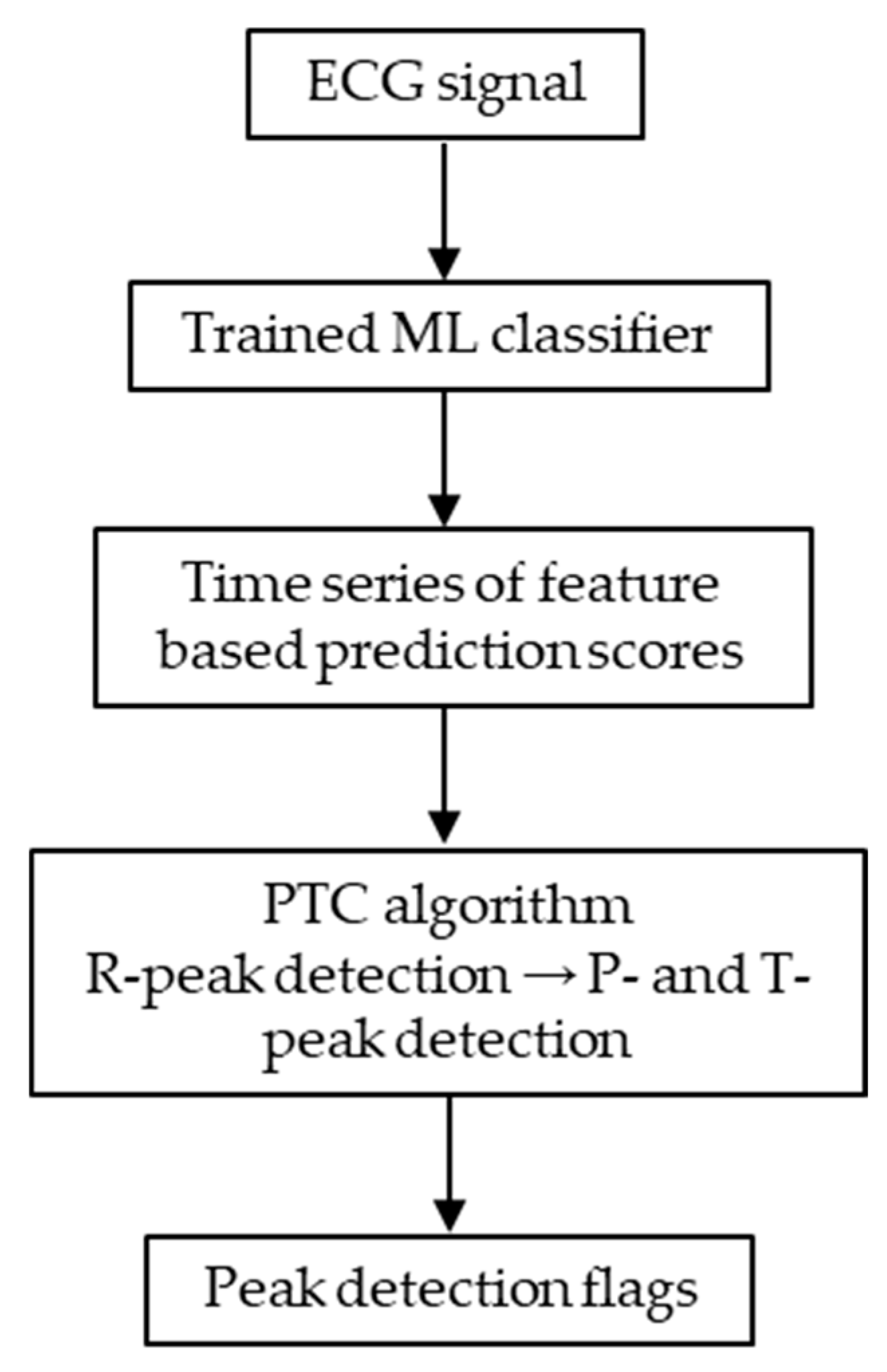
Figure 2.
ROC curves of each classifier. The horizontal axis represents the FP rate, and the vertical axis represents the TP rate. Green: R-peak; orange: P-peak; red: T-peak.
Figure 2.
ROC curves of each classifier. The horizontal axis represents the FP rate, and the vertical axis represents the TP rate. Green: R-peak; orange: P-peak; red: T-peak.
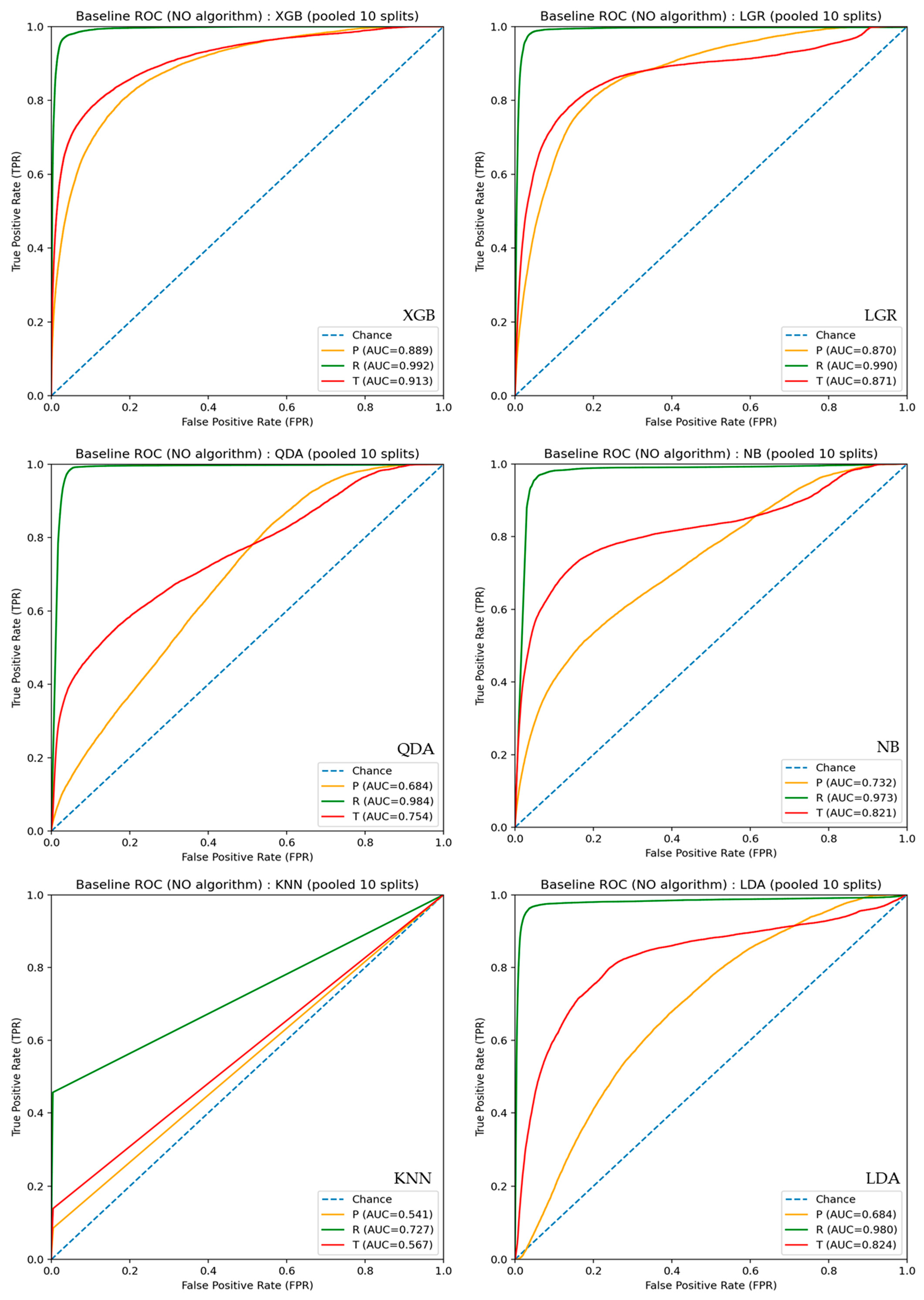
Figure 3.
PR curves of each classifier. The horizontal axis represents recall, and the vertical axis represents precision. Green: R-peak; orange: P-peak; red: T-peak.
Figure 3.
PR curves of each classifier. The horizontal axis represents recall, and the vertical axis represents precision. Green: R-peak; orange: P-peak; red: T-peak.
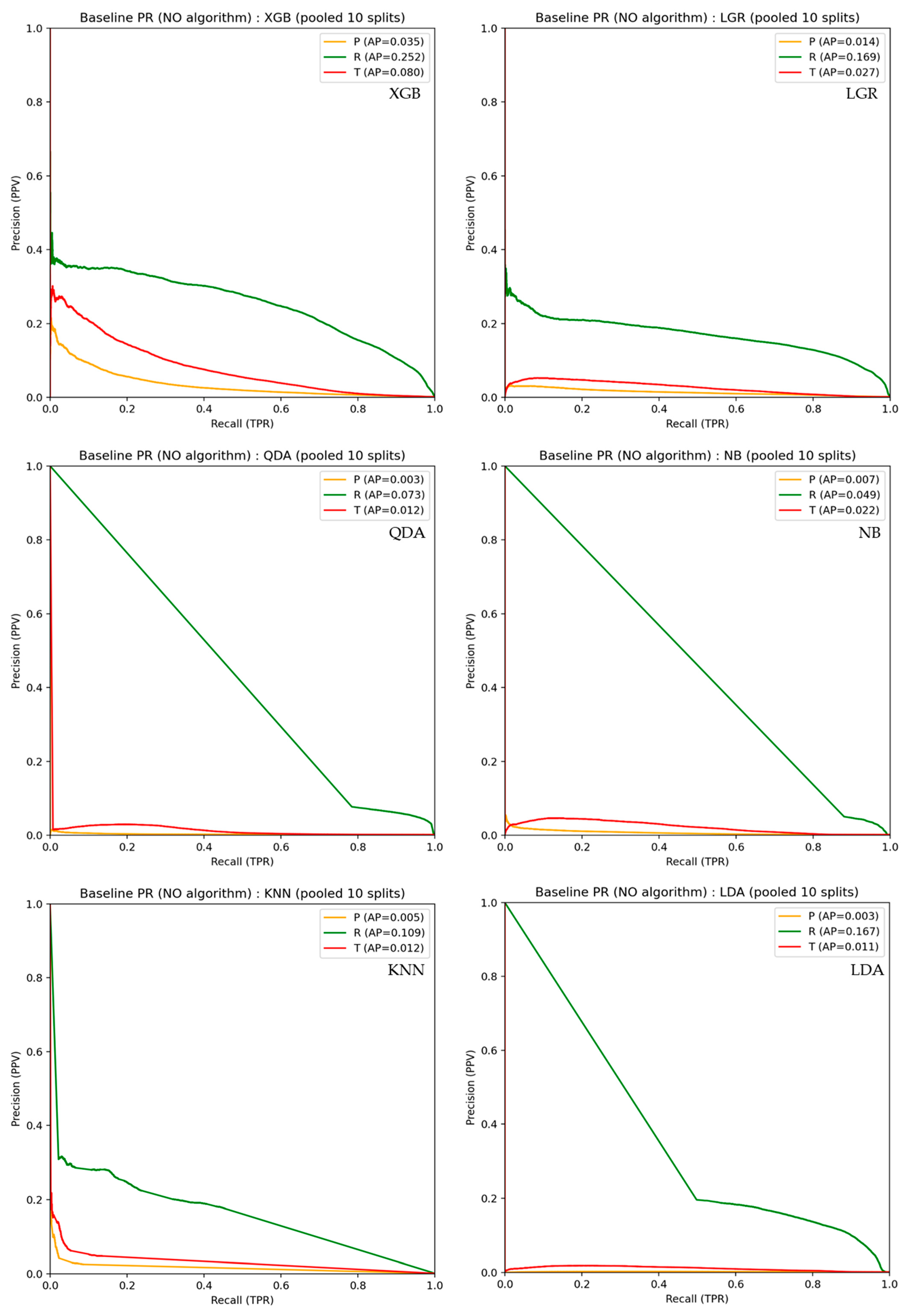
Figure 4.
Effect of the HPF cutoff frequency on peak detection performance(tol=±20 ms). Se, PPV, and F1 for P-, R-, and T-peak detection are shown under different CFH settings. ■: R-peak, ■: P-peak, ■: T-peak.
Figure 4.
Effect of the HPF cutoff frequency on peak detection performance(tol=±20 ms). Se, PPV, and F1 for P-, R-, and T-peak detection are shown under different CFH settings. ■: R-peak, ■: P-peak, ■: T-peak.
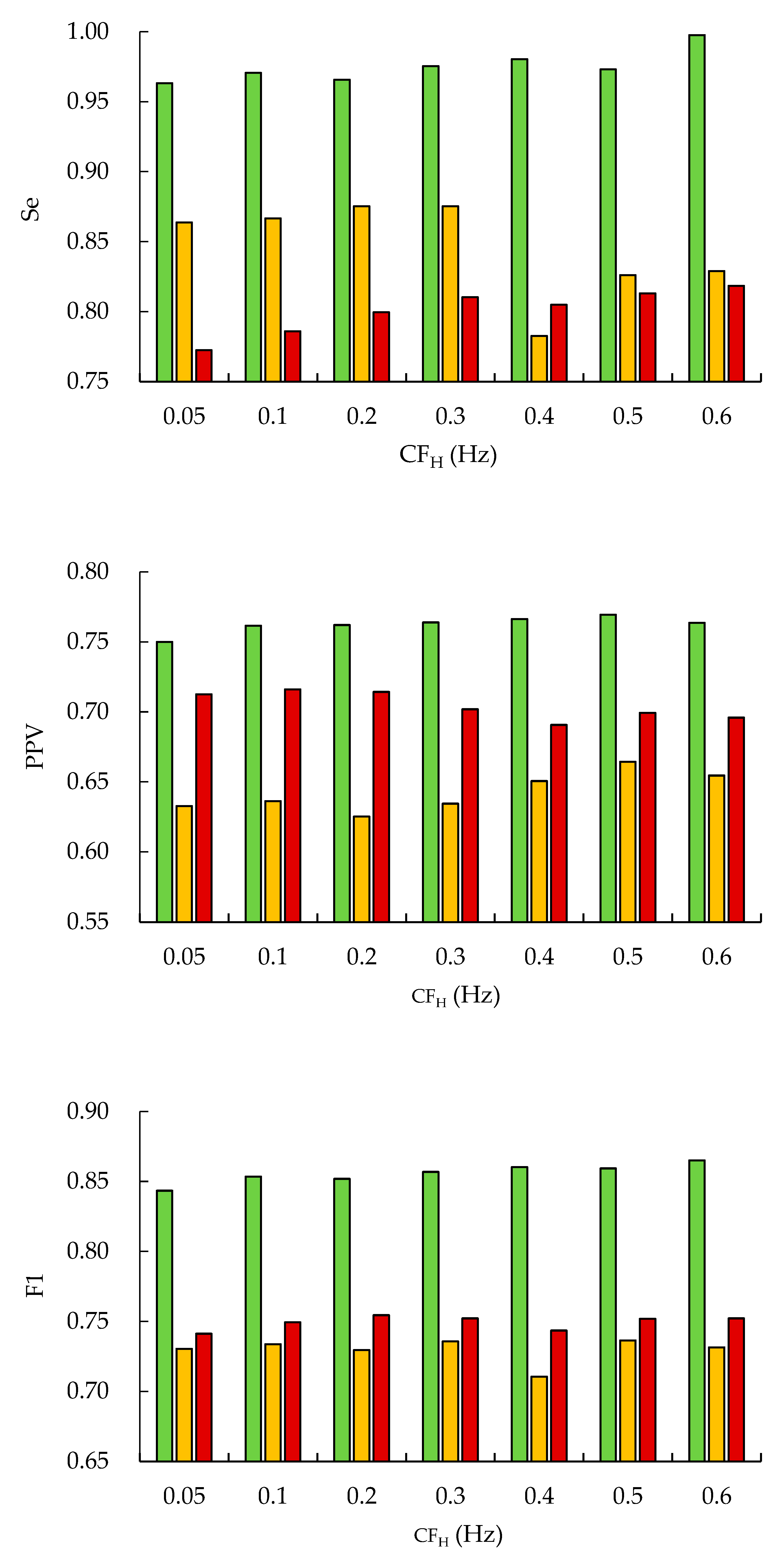
Figure 5.
Peak detection results of SR ECG signals from PTB-XL. Upper: ID 005; lower: ID 014, ●: R-peak, ▼: P-peak, ▼: T-peak.
Figure 5.
Peak detection results of SR ECG signals from PTB-XL. Upper: ID 005; lower: ID 014, ●: R-peak, ▼: P-peak, ▼: T-peak.
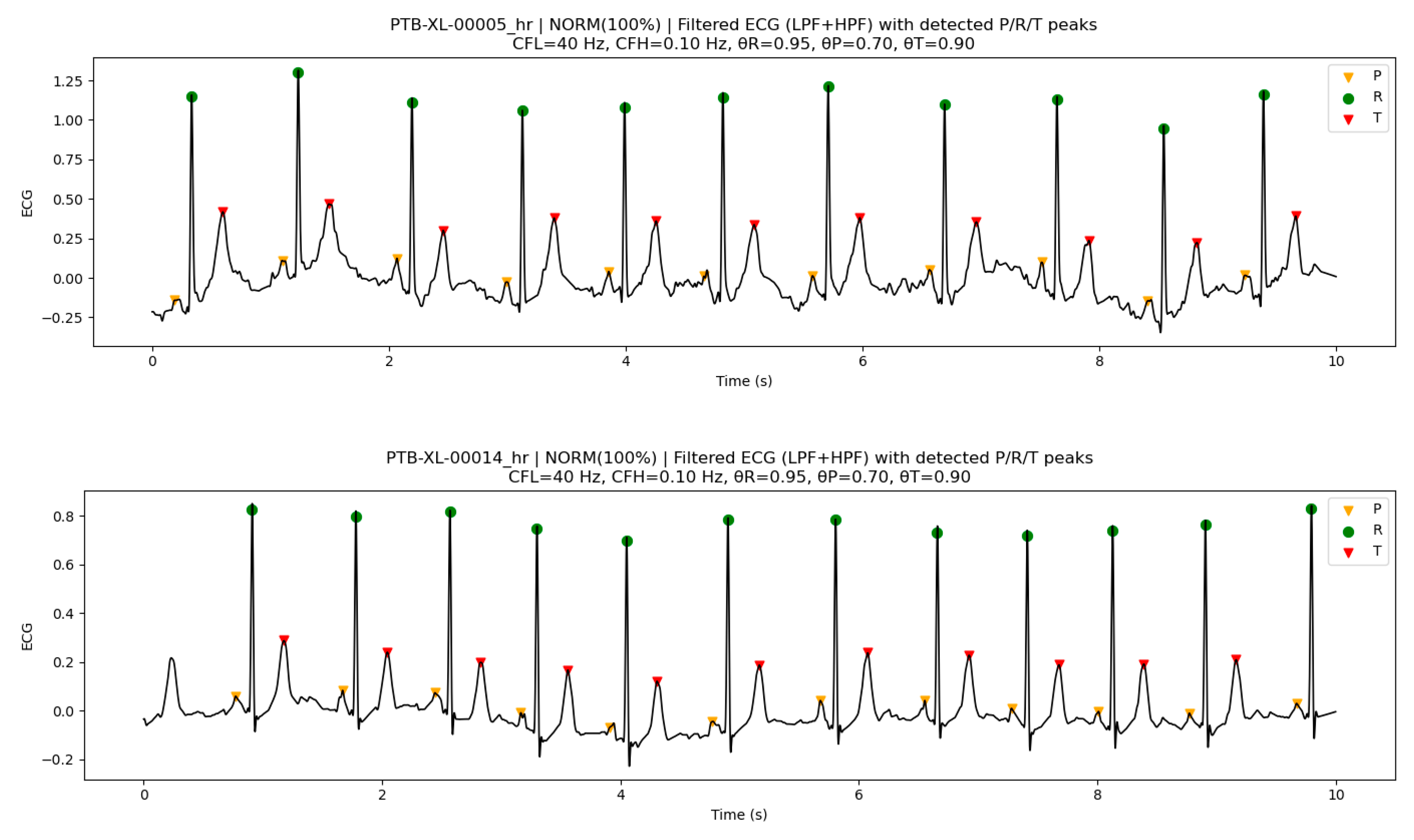
Figure 6.
An example with rich high-frequency components (ID 001, SR). Upper:CFL=40Hz, lower: CFL=16Hz, ●:R-peak, ▼:P-peak, ▼:T-peak.
Figure 6.
An example with rich high-frequency components (ID 001, SR). Upper:CFL=40Hz, lower: CFL=16Hz, ●:R-peak, ▼:P-peak, ▼:T-peak.
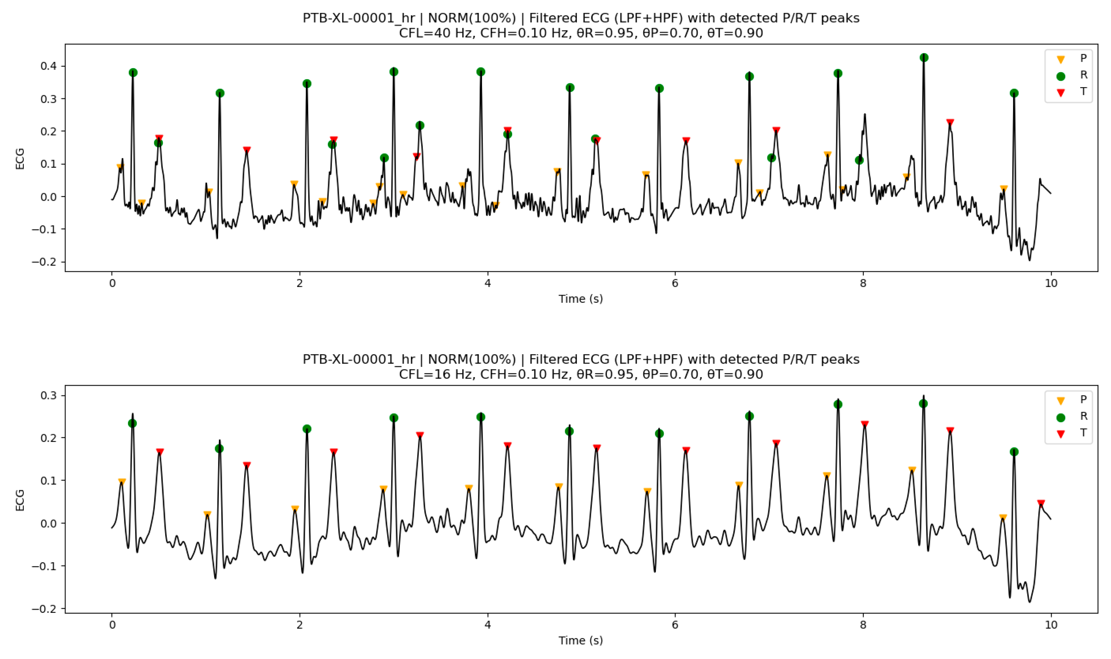
Figure 7.
An example with large variations in baseline drift (ID 008, IMI). Upper: CFH=0.10Hz, lower: CFH=0.30Hz, ●:R-peak, ▼:P-peak, ▼:T-peak.
Figure 7.
An example with large variations in baseline drift (ID 008, IMI). Upper: CFH=0.10Hz, lower: CFH=0.30Hz, ●:R-peak, ▼:P-peak, ▼:T-peak.
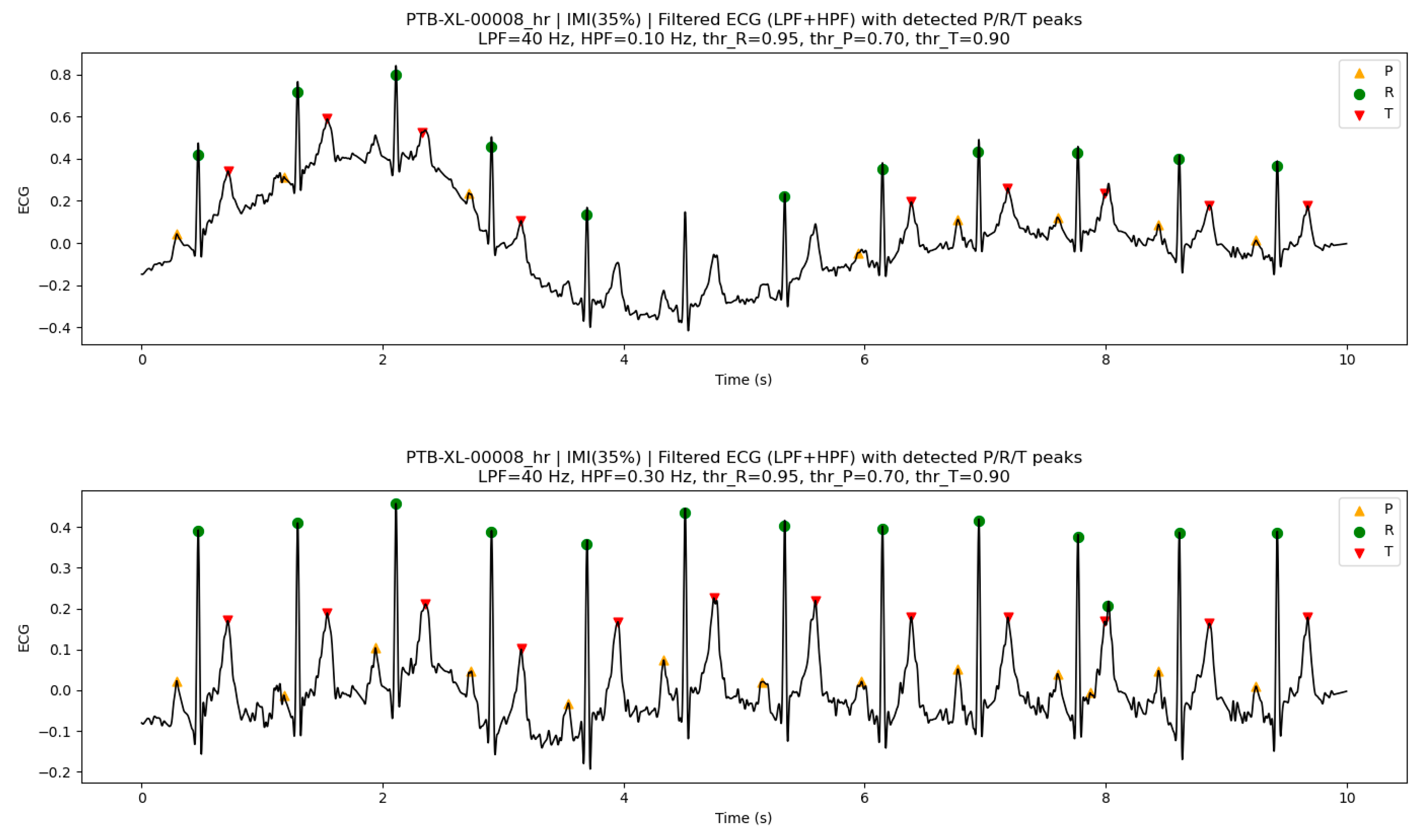
Figure 8.
Examples of peak detection in AFLT. Upper: ID 017; lower: ID 018, ●:R-peak, ▼:P-peak, ▼:T-peak.
Figure 8.
Examples of peak detection in AFLT. Upper: ID 017; lower: ID 018, ●:R-peak, ▼:P-peak, ▼:T-peak.
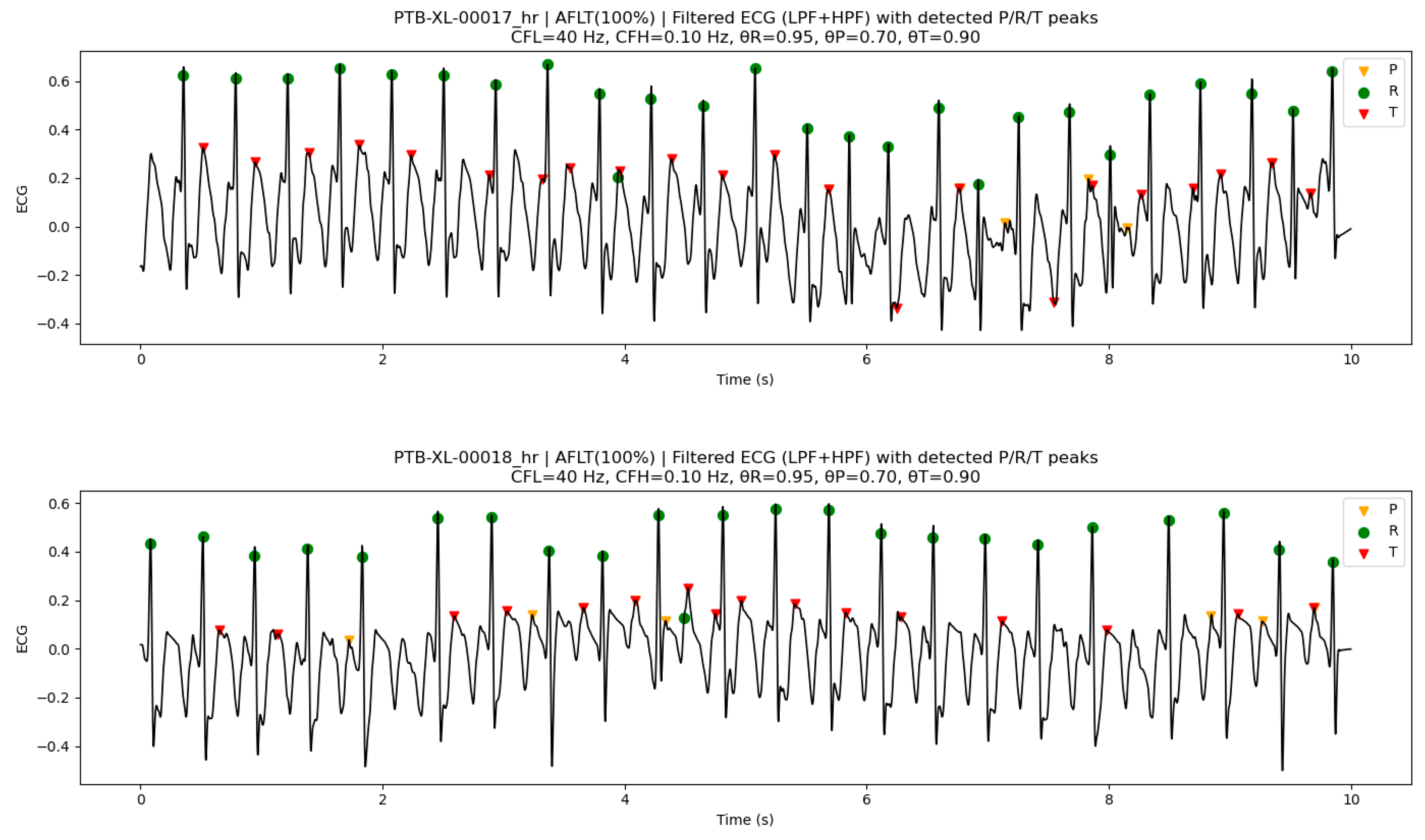

Table 1.
Example of R-peak selection with refractory-period suppression (10 steps, Refractory period = 50 ms).
Table 1.
Example of R-peak selection with refractory-period suppression (10 steps, Refractory period = 50 ms).
| Step | Candidate time (ms) |
Score | Previously selected R-peaks (ms) |
Distance to nearest selected peak (ms) |
Decision | Reason |
| 1 | 1600 | 0.99 | — | — | Adopt | First peak, highest score |
| 2 | 800 | 0.97 | [1600] | 800 (>50) | Adopt | Far from 1600 ms |
| 3 | 1635 | 0.94 | [800,1600] | 35 (≤50) | Reject | Within refractory of 1600 ms |
| 4 | 2400 | 0.92 | [800,1600] | 800 (>50) | Adopt | New beat |
| 5 | 770 | 0.88 | [800,1600,2400] | 30 (≤50) | Reject | Within refractory of 800 ms |
| 6 | 3220 | 0.85 | [800,1600,2400] | 820 (>50) | Adopt | New beat |
| 7 | 3270 | 0.8 | [800,1600,2400,3220] | 50 (≤50) | Reject | Within refractory of 3220 ms |
| 8 | 4020 | 0.76 | [800,1600,2400,3220] | 800 (>50) | Adopt | Distant new beat |
| 9 | 2370 | 0.71 | [800,1600,2400,3220,4020] | 30 (≤50) | Reject | Within refractory of 2400 ms |
| 10 | 4820 | 0.68 | [800,1600,2400,3220,4020] | 800 (>50) | Adopt | New beat |
Table 2.
AUC and AP of each classifier before incorporating the PTC algorithm.
| Classifier | P-peak | R-peak | T-peak | |||
| AUC | AP | AUC | AP | AUC | AP | |
| XGB | 0.889 | 0.035 | 0.992 | 0.252 | 0.913 | 0.080 |
| LGR | 0.870 | 0.014 | 0.990 | 0.169 | 0.871 | 0.027 |
| QDA | 0.684 | 0.003 | 0.984 | 0.073 | 0.754 | 0.012 |
| NB | 0.732 | 0.007 | 0.973 | 0.049 | 0.821 | 0.022 |
| KNN | 0.541 | 0.005 | 0.727 | 0.109 | 0.567 | 0.012 |
| LDA | 0.684 | 0.003 | 0.980 | 0.167 | 0.824 | 0.011 |
Table 3.
Peak detection performance after incorporating the PTC algorithm.
| Classifier | R-peak (tol=±20 ms) | ||||||
| N (Total ECG time points) |
Se | PPV | F1 | TP | FP | FN | |
| XGB | 225000 | 0.963±0.038 | 0.787±0.025 | 0.866±0.026 | 397±24 | 108±14 | 15±16 |
| LGR | 225000 | 0.955±0.046 | 0.785±0.029 | 0.861±0.035 | 394±25 | 111±19 | 18±17 |
| QDA | 225000 | 0.932±0.064 | 0.755±0.033 | 0.834±0.041 | 384±32 | 124±18 | 28±26 |
| NB | 225000 | 0.918±0.040 | 0.750±0.031 | 0.826±0.033 | 378±24 | 126±15 | 34±16 |
| KNN | 225000 | 0.524±0.056 | 0.796±0.023 | 0.63±0.042 | 224±16 | 58±8 | 188±11 |
| LDA | 225000 | 0.945±0.056 | 0.813±0.01 | 0.873±0.026 | 389±29 | 89±6 | 23±23 |
| Classifier | P-peak (tol=±20 ms) | ||||||
| N (Total ECG time points) |
Se | PPV | F1 | TP | FP | FN | |
| XGB | 225000 | 0.794±0.055 | 0.626±0.025 | 0.699±0.032 | 275±22 | 177±24 | 81±24 |
| LGR | 225000 | 0.804±0.048 | 0.588±0.041 | 0.679±0.042 | 283±20 | 198±23 | 73±13 |
| QDA | 225000 | 0.669±0.062 | 0.489±0.048 | 0.565±0.052 | 245±26 | 244±20 | 110±20 |
| NB | 225000 | 0.631±0.05 | 0.46±0.031 | 0.532±0.037 | 235±16 | 254±18 | 121±26 |
| KNN | 225000 | 0.162±0.034 | 0.485±0.08 | 0.242±0.043 | 49±10 | 71±24 | 307±22 |
| LDA | 225000 | 0 | - | 0 | 0 | 0 | 356±23 |
| Classifier | T-peak (tol=±20 ms) | ||||||
| N (Total ECG time points) |
Se | PPV | F1 | TP | FP | FN | |
| XGB | 225000 | 0.766±0.064 | 0.629±0.057 | 0.69±0.055 | 279±23 | 177±38 | 90±23 |
| LGR | 225000 | 0.769±0.071 | 0.607±0.059 | 0.678±0.062 | 279±32 | 170±27 | 91±28 |
| QDA | 225000 | 0.670±0.074 | 0.503±0.047 | 0.575±0.057 | 258±26 | 233±28 | 111±27 |
| NB | 225000 | 0.755±0.058 | 0.568±0.048 | 0.648±0.051 | 282±23 | 207±20 | 87±19 |
| KNN | 225000 | 0.253±0.041 | 0.523±0.041 | 0.339±0.041 | 91±8 | 95±9 | 279±18 |
| LDA | 225000 | 0.041±0.025 | 0.568±0.131 | 0.075±0.044 | 15±9 | 10±4 | 355±20 |
Table 4.
Peak detection performance of XGB and LGR at tol = ±10 ms and ±30 ms.
| Classifier | R-peak (tol_10ms) | R-peak (tol_30ms) | ||||
| Se | PPV | F1 | Se | PPV | F1 | |
| XGB | 0.946±0.050 | 0.773±0.033 | 0.85±0.037 | 0.964±0.037 | 0.787±0.026 | 0.867±0.026 |
| LGR | 0.937±0.059 | 0.769±0.037 | 0.845±0.045 | 0.966±0.033 | 0.794±0.026 | 0.872±0.026 |
| Classifier | P-peak (tol_10ms) | P-peak (tol_30ms) | ||||
| Se | PPV | F1 | Se | PPV | F1 | |
| XGB | 0.698±0.047 | 0.551±0.025 | 0.615±0.029 | 0.844±0.061 | 0.666±0.023 | 0.744±0.034 |
| LGR | 0.692±0.043 | 0.506±0.031 | 0.585±0.033 | 0.87±0.047 | 0.636±0.037 | 0.734±0.037 |
| Classifier | T-peak (tol_10ms) | T-peak (tol_30ms) | ||||
| Se | PPV | F1 | Se | PPV | F1 | |
| XGB | 0.681±0.057 | 0.559±0.054 | 0.613±0.051 | 0.799±0.061 | 0.656±0.054 | 0.719±0.051 |
| LGR | 0.675±0.065 | 0.533±0.051 | 0.595±0.055 | 0.809±0.069 | 0.639±0.059 | 0.714±0.061 |
Table 5.
Summary of optimized algorithmic parameters and score threshold across classifiers. Values are reported as median [min–max], with the most frequent value (mode) in parentheses.
Table 5.
Summary of optimized algorithmic parameters and score threshold across classifiers. Values are reported as median [min–max], with the most frequent value (mode) in parentheses.
| Classifier | win_len | refR (ms) | θR |
| XGB | 15 [13–15] (15) | 60 [40–80] (60) | 0.95 [0.60–0.95] (0.95) |
| LGR | 7 [7–15] (7) | 55 [30–80] (40) | 0.85 [0.65–0.90] (0.90) |
| QDA | 11 [9–15] (11) | 80 [70–80] (80) | 0.60 [0.45–1.00] (0.60) |
| NB | 7 [7–11] (7/9) | 75 [40–80] (80) | 0.55 [0.40–0.90] (0.55) |
| KNN | 9 [7–15] (9) | 30 [30–30] (30) | 0.40 [0.40–0.40] (0.40) |
| LDA | 7 [7–15] (7) | 40 [30–80] (40) | 0.40 [0.40–0.55] (0.40) |
| Classifier | θP | θT | |
| XGB | 0.70 [0.40–0.80] (0.70) | 0.70 [0.05–0.90] (0.80) | |
| LGR | 0.50 [0.05–0.60] (0.50) | 0.50 [0.05–0.50] (0.50) | |
| QDA | 0.05 [0.05–0.90] (0.05) | 0.05 [0.05–0.90] (0.05) | |
| NB | 0.80 [0.05–0.90] (0.90) | 0.05 [0.05–0.90] (0.05) | |
| KNN | 0.05 [0.05–0.05] (0.05) | 0.05 [0.05–0.05] (0.05) | |
| LDA | 0.05 [0.05–0.05] (0.05) | — |
Table 6.
Optimized P- and T-peak algorithmic parameters (median [min–max] (mode)).
| Classifier | Ppre (ms) | Ppost (ms) | Tpre (ms) | Tpost (ms) |
| XGB | 100 [80–100] (100) | 200 [180–240] (200) | 120 [100–120] (120) | 350 [300–450] (350) |
| LGR | 100 [100–100] (100) | 240 [200–240] (200) | 120 [60–120] (120) | 350 [300–450] (350) |
| QDA | 100 [100–100] (100) | 180 [160–200] (180) | 120 [80–120] (120) | 350 [300–450] (350) |
| NB | 100 [80–100] (100) | 220 [180–220] (220) | 120 [80–120] (120) | 350 [300–400] (350) |
| kNN | 40 [40–100] (40) | 220 [180–260] (200) | 40 [40–120] (40) | 350 [350–450] (350) |
| LDA | — | — | 40 [40–120] (40) | 300 [300–400] (300) |
Table 7.
Summary of optimized classifier parameters (median [min–max] (mode)).
| Classifier | Parameter | P-peak | R-peak | T-peak |
| XGB | n_estimators | 300 [300–300] (300) | 300 [300–300] (300) | 300 [300–300] (300) |
| max_depth | 4 [4–4] (4) | 4 [4–4] (4) | 4 [4–4] (4) | |
| learning_rate | 0.1 [0.1–0.1] (0.1) | 0.1 [0.1–0.1] (0.1) | 0.1 [0.1–0.1] (0.1) | |
| LGR | C | 10 [1–10] (10) | 0.1 [0.1–1] (0.1/1) | 10 [0.1–10] (10) |
| KNN | n_neighbors | 3 [3–8] (3) | 3 [3–8] (3) | 3 [3–3] (3) |
Table 8.
Performance evaluation of XGB for peak detection on arrhythmic LUDB data. The results in this table were calculated using parameter settings optimized on SR data. The algorithmic parameters were fixed as {win_len = 15, θR = 0.95, refR = 60 ms, Ppre = 200 ms, Ppost = 100 ms, θP = 0.70, Tpre = 120 ms, Tpost = 350 ms, θT = 0.80}, and the classifier hyperparameters were set to {n_estimators = 300, max_depth = 4, learning_rate = 0.1}.
| Peak | N (Total ECG time points) |
Se | PPV | F1 | TP | FP | FN |
| R | 867564 | 0.931 | 0.764 | 0.839 | 1509 | 466 | 111 |
| P | 867564 | 0.786 | 0.414 | 0.542 | 684 | 970 | 186 |
| T | 867564 | 0.645 | 0.582 | 0.612 | 937 | 672 | 515 |
Table 9.
F1 for each peak detection across different arrhythmia types. The F1 values are sorted in descending order for each peak.
Table 9.
F1 for each peak detection across different arrhythmia types. The F1 values are sorted in descending order for each peak.
| Arrhythmia | R-peak | Arrhythmia | P-peak | Arrhythmia | T-peak |
| SNT | 0.935 | SNT | 0.867 | SRW | 0.882 |
| SRW | 0.917 | SNA | 0.786 | SAW | 0.842 |
| AFA | 0.905 | SAW | 0.750 | SNA | 0.807 |
| SNA | 0.904 | SR | 0.727 | SR | 0.769 |
| SR | 0.902 | SNB | 0.625 | SNT | 0.740 |
| SAW | 0.900 | ISN | 0.598 | ISN | 0.729 |
| ISN | 0.870 | SRW | 0.324 | TAF | 0.677 |
| AFLT | 0.857 | SBW | 0.320 | SNB | 0.655 |
| SNB | 0.844 | AF | 0.000 | AFLT | 0.352 |
| AF | 0.746 | AFA | 0.000 | AFA | 0.206 |
| SBW | 0.727 | AFLT | 0.000 | SBW | 0.000 |
Table 10.
Detailed P-peak detection results for AF–related rhythms.
| Arrhythmia | N (Total ECG time points) |
PPV | Se | F1 | TP | FP | FN | FP/N (%) |
| AF | 209412 | 0 | 0 | 0 | 0 | 353 | 0 | 0.169 |
| AFA | 14958 | 0 | 0 | 0 | 0 | 43 | 0 | 0.287 |
| AFLT | 44874 | 0 | 0 | 0 | 0 | 136 | 0 | 0.303 |
Table 11.
Selected PTC algorithm and classifier parameters for CFH (0.05–0.3 Hz). The classifier hyperparameters were fixed, whereas the PTC algorithm parameters were optimized for each preprocessing condition.
Table 11.
Selected PTC algorithm and classifier parameters for CFH (0.05–0.3 Hz). The classifier hyperparameters were fixed, whereas the PTC algorithm parameters were optimized for each preprocessing condition.
| Parameters | CFH (Hz) | |||
| 0.05 | 0.1 | 0.2 | 0.3 | |
| win_len | 15 | 15 | 13 | 15 |
| refR (ms) | 50 | 50 | 40 | 30 |
| θR | 0.95 | 0.95 | 0.95 | 0.95 |
| θP | 0.7 | 0.7 | 0.6 | 0.6 |
| θT | 0.9 | 0.9 | 0.9 | 0.9 |
| Ppre (ms) | 200 | 200 | 200 | 200 |
| Ppost (ms) | 100 | 100 | 100 | 100 |
| Tpre (ms) | 120 | 120 | 120 | 60 |
| Tpost (ms) | 450 | 450 | 450 | 450 |
| n_estimators | 300 | 300 | 300 | 300 |
| max_depth | 4 | 4 | 4 | 4 |
| learning_rate | 0.1 | 0.1 | 0.1 | 0.1 |
Disclaimer/Publisher’s Note: The statements, opinions and data contained in all publications are solely those of the individual author(s) and contributor(s) and not of MDPI and/or the editor(s). MDPI and/or the editor(s) disclaim responsibility for any injury to people or property resulting from any ideas, methods, instructions or products referred to in the content. |
© 2026 by the authors. Licensee MDPI, Basel, Switzerland. This article is an open access article distributed under the terms and conditions of the Creative Commons Attribution (CC BY) license (http://creativecommons.org/licenses/by/4.0/).
Copyright: This open access article is published under a Creative Commons CC BY 4.0 license, which permit the free download, distribution, and reuse, provided that the author and preprint are cited in any reuse.


