Submitted:
06 February 2026
Posted:
09 February 2026
You are already at the latest version
Abstract
Maintaining stable temperature and relative humidity (RH) is critical for edible fungi cultivation, yet the climate dynamics are nonlinear and strongly coupled, making conventional control prone to slow recovery under disturbances. This study develops a reproducible lumped-parameter coupled temperature–humidity model and validates a fuzzy-PID strategy in MATLAB/Simulink through numerical experiments. The model describes the thermal and moisture dynamics using effective capacities and aggregated heat/moisture exchange terms. Three standardized scenarios are designed for repeatable evaluation: set-point tracking, step disturbances (±2 °C and ±5% RH), and periodic disturbances. The proposed fuzzy-PID is compared with a baseline PID and a no-control case using unified control metrics (steady-state error, settling time, recovery time, integral error) and total energy consumption. Under the same disturbance settings, fuzzy-PID achieves faster recovery and lower error accumulation than PID, while reducing total energy consumption (e.g., 5.7 kWh vs 6.7 kWh for PID in a representative test). These results demonstrate that the proposed modeling and control framework is reproducible and suitable for simulation-based assessment of controllers during high-humidity cultivation stages.
Keywords:
edible fungi
; cultivation room
; coupled dynamics
; temperature and humidity control
; fuzzy-PID
; MATLAB/Simulink
; disturbance rejection
1. Introduction
Edible fungi cultivation requires a stable microclimate because both yield and quality are highly sensitive to environmental fluctuations. Among the controllable factors, temperature and relative humidity (RH) are the two most critical variables, and they must be regulated within appropriate ranges to maintain favorable growth conditions over long cultivation periods. However, the cultivation room climate is influenced by nonlinear heat and moisture transfer processes, external disturbances (e.g.; ventilation and ambient changes), and actuator constraints, which can lead to slow responses, steady-state deviations, and unnecessary energy consumption in practice.
A key engineering challenge is the intrinsic coupling between temperature and RH: temperature variations change the air’s moisture-holding capacity and thus RH, while humidification and ventilation processes modify moisture content and can also affect the thermal state. Therefore, independent single-loop tuning may lead to cross-effects between the two variables and reduced disturbance-rejection capability. These characteristics underscore the need for a modeling-and-control framework that can be evaluated under standardized, reproducible conditions.
In this study, a coupled temperature–humidity dynamic model is established, and a fuzzy-PID strategy is assessed in MATLAB/Simulink through reproducible numerical experiments. The proposed approach is compared with a baseline PID and a no-control case under set-point tracking, step disturbances, and periodic disturbances, using unified performance metrics such as tracking error, settling/recovery behavior, and total energy consumption. The results provide a simulation-based and reproducible reference for controller assessment in edible fungi cultivation rooms [1,2,3].
2. Analysis of Temperature and Humidity Requirements and Coupling Mechanism for Edible Fungi Growth
2.1. Growth Stages of Edible Fungi and Environmental Requirements
The cultivation process of edible fungi can be generally described by several stages (e.g.; germination, mycelial growth, fruiting, and maturation), and the environmental requirements may vary across stages and species. For reproducibility in this paper, we focus on a representative high-humidity cultivation condition used in the subsequent control tests, and set the set-points to T=22℃ and RH=90% throughout the simulation study. This setting enables consistent comparisons of different control strategies under identical operating conditions and disturbance profiles, and it underscores the need for precise, coordinated regulation of temperature and relative humidity to improve cultivation performance [4,5].
2.2. Physical Relationship and Coupling Characteristics Between Temperature and Relative Humidity
There exists a close physical coupling relationship between temperature and relative humidity. Temperature affects the air’s saturation capacity for water vapor, while relative humidity depends on both temperature and the actual water vapor content. Specifically, relative humidity (RH) can be expressed as the ratio of the actual water vapor pressure at the same temperature:
where e is the actual vapor pressure and is the saturation vapor pressure at temperature T. As temperature changes, changes nonlinearly, so RH may vary significantly even when the absolute moisture content is unchanged. In edible fungi cultivation, such coupling means that regulating temperature may induce changes in RH, and humidification/ventilation may also influence thermal conditions. Therefore, controlling a single factor independently may lead to cross-effects and make it difficult to maintain an optimal growth environment under disturbances; both factors should be considered jointly in control [6,7].
Figure 1.
Coupled Temperature and humidity Relationship Model.
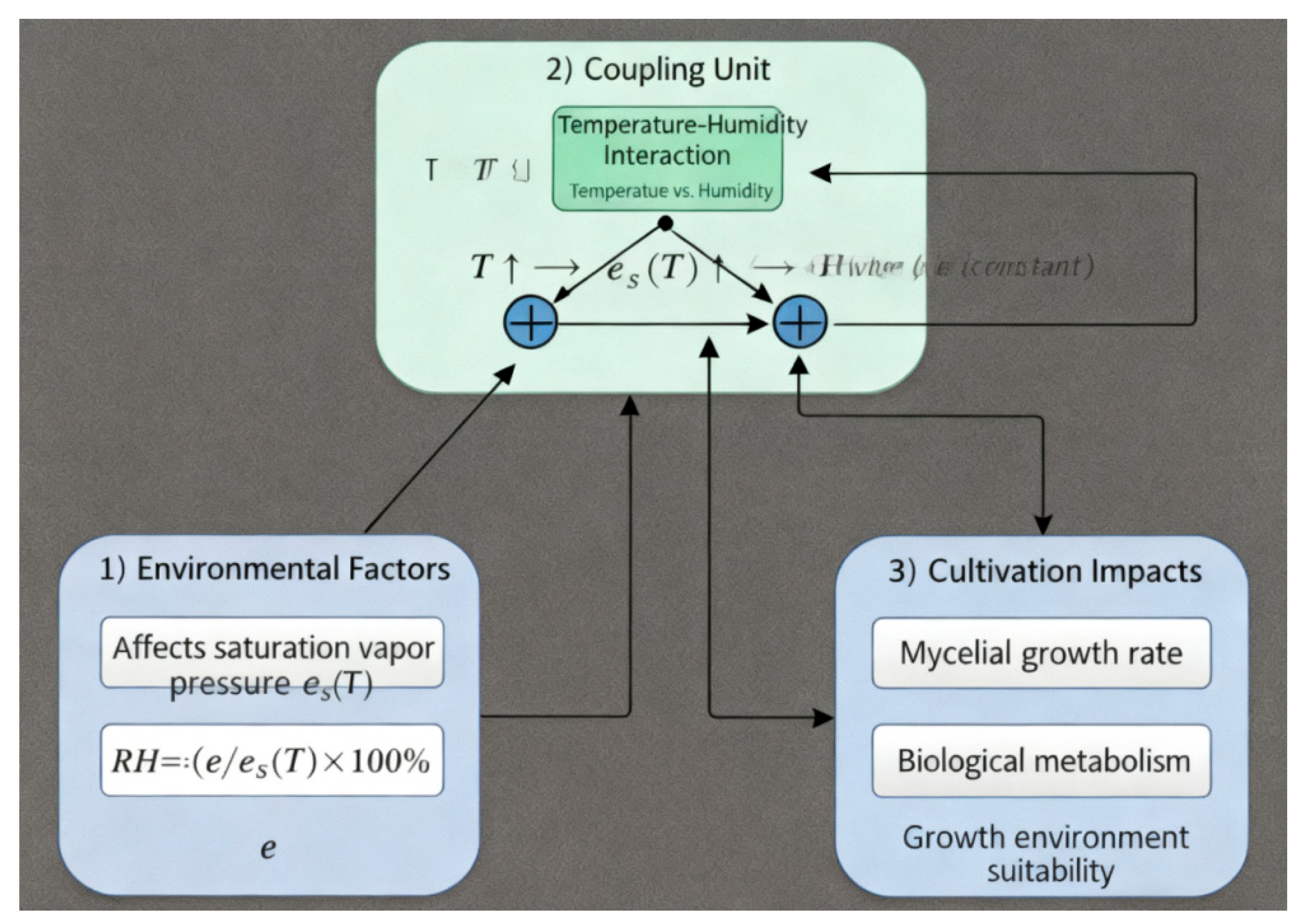
2.3. Mechanism Model of the Effect of Temperature and Humidity on Mycelial Growth Rate
Temperature and humidity affect mycelial growth by influencing metabolic activity, hydration status, and gas exchange conditions [11,12]. Extreme temperature conditions may reduce growth by slowing metabolism, while excessively low RH can cause dehydration and stall growth; conversely, overly high RH may increase surface wetness and reduce effective ventilation, limiting oxygen availability.
where r(T, H)is the mycelial growth rate at coupled T and H, rmax is the maximum specific growth rate, Topt and Hopt are the optimal values of T and H, and σT and σH represent the sensitivities of r(T, H) to T and H, respectively. This model shows that temperature and humidity have coupled effects on mycelial growth, meaning that the effects of both factors on the mycelial growth rate decrease when their values deviate from optimal values.
3. Construction of the Temperature-Humidity Coupling Mathematical Model
3.1. Construction of the Environmental Temperature-Humidity Dynamics Model
The goal of the temperature–humidity dynamics model is to describe the temporal variation of temperature and humidity and their interactions [8]. A reproducible lumped-parameter model is adopted by considering the heat and water-vapor exchange in the room air. The coupled dynamics are expressed as:
where T(t) is the indoor air temperature and H(t) denotes indoor humidity ; Qin(t) and Qout(t) are the aggregated heat gain and heat loss terms (e.g.; heating input, ventilation loss, heat exchange with the envelope); Ein(t) and Eout(t) are the aggregated moisture gain and moisture loss terms (e.g.; humidification/evaporation input and ventilation/dehumidification loss). CT and CH represent effective thermal and moisture capacities, respectively. This formulation follows energy and mass conservation principles and enables the simulation of temperature and humidity variations under different external disturbances (e.g.; changes in heat sources, changes in evaporation rates, ventilation effects) and control inputs.
3.2. Coupled Temperature-Humidity Growth Model and System Coupling Structure Design
The impact of temperature and humidity on the growth of edible fungi should be comprehensively characterized using a system-level coupling model [9,10]. Based on the growth-rate relationship described in Section 2.3 and the temperature–humidity dynamic equations in Section 3.1, a coupled temperature–humidity growth model can be constructed by treating environmental temperature and humidity as system inputs and the mycelial growth rate as the output. The coupled model can be written in a compact form as:
where is the mycelial growth rate and represents the coupled effect of dynamic temperature and humidity on growth.
For the system coupling structure, the control objective is to regulate and (or RH) to their set-points under disturbances, so that r(t) remains close to its optimal region. In practice, the coupling structure should include sensor feedback (temperature and humidity measurements), a controller that computes control actions (heating/humidification/ventilation), and the dynamic model that describes how the environment responds to control inputs and external disturbances. This closed-loop coupling structure supports real-time adjustment of temperature and humidity to maintain a favorable growth environment and improve cultivation performance [11,12,13].
4. Temperature-Humidity Coupling Control Strategy Design
4.1. Analysis of the Mimo (Multiple Input Multiple Output) Control System
The temperature–humidity coupling system can be regarded as a multivariable regulation problem because temperature and relative humidity are distinct variables but exhibit strong cross-effects. In such systems, independent adjustment of one variable may inadvertently perturb the other, increasing control difficulty and motivating coordinated regulation. Therefore, the controller design should explicitly account for the interaction between temperature and humidity to reduce cross-coupling and improve disturbance rejection [14].
In principle, advanced multivariable methods (e.g.; model predictive control and adaptive control) can be used to coordinate coupled variables when a sufficiently accurate model and constraints are available. However, for a reproducible and implementable baseline, this study focuses on comparing classical PID and fuzzy-PID strategies under standardized simulation scenarios, while leaving advanced multivariable optimization as an extension [15,16,17].
4.2. Fuzzy-Pid Controller Design
A traditional PID controller is simple and effective; however, in a coupled temperature–humidity system with disturbances and nonlinearities, PID may suffer from slow recovery and limited adaptability. To enhance robustness, fuzzy supervision is integrated with PID to form a fuzzy-PID controller. In this study, two independent fuzzy-PID controllers are implemented for the temperature and relative humidity loops (SISO×2), enabling reproducible implementation and a fair comparison with the baseline PID.
In each loop, the fuzzy supervisor takes the tracking error e and its change Δe as inputs. After normalization to [−1,1], five linguistic terms {NB, NS, ZO, PS, PB} with triangular membership functions are used. The fuzzy rule base outputs the control increment Δu (equivalently, the PID adjustment), and the final crisp output is obtained via centroid defuzzification. The resulting control action is updated discretely as u(k) = u(k−1) + Δu (k). This design does not require an exact mathematical model and can respond quickly to uncertainties and disturbances [18].
5. Simulation Experiment Design and Implementation
5.1. Simulation Environment and Parameter Design
To evaluate the proposed temperature–humidity coupling control strategy under reproducible conditions, all experiments are conducted on the MATLAB/Simulink platform. The coupled dynamic model (Section 3) and the control strategies (Section 4) are implemented in a closed-loop simulation, with the controlled variables being indoor temperature T(t) and relative humidity RH(t). The simulation adopts a fixed sampling time Δt = [1 s ] and a total simulation duration Tsim = 40 min for each scenario. To ensure fair comparisons, all controllers share identical model parameters and disturbance profiles. The baseline comparison includes: (i) no-control case, (ii) classical PID, and (iii) fuzzy-PID.
Key simulation parameters are listed in Table 1 (temperature setting range 18–28 °C, RH setting range 80–95%, air heat capacity 1.0 J/(kg·K), evaporation rate 0.05 kg/s, and external disturbance amplitudes ±2 °C and ±5% RH). These settings are used to reproduce typical high-humidity cultivation conditions in a numerical environment and to test controller performance consistently across different disturbances..
By adjusting these parameters, the simulation can model the performance of the temperature-humidity control system under different external conditions. These parameter settings not only reflect the system’s response to various control strategies but also help analyze the effects of temperature-humidity control under different operating conditions.
5.2. Simulation Operating Conditions and Disturbance Scenario Setting
To verify the effectiveness of the temperature–humidity coupling control strategy, standardized operating conditions and disturbance scenarios are designed in simulation. The experiments include nominal operation and two reproducible disturbance types: (i) sudden (step) disturbances and (ii) periodic disturbances.
For sudden disturbances, the external temperature step change is set to ±2 °C, and the external RH step change is set to ±5%. For periodic disturbances, sinusoidal disturbance signals with the same amplitudes are applied to emulate cyclic environmental variations. These disturbance profiles are injected into the model as external inputs so that all controllers are tested under identical interference conditions.
5.3. Simulation Process and System Response
The closed-loop simulation follows four functional modules: (1) signal sampling, (2) error computation, (3) control decision, and (4) feedback update. At each sampling time k, the model outputs T(k) and RH(k). The tracking errors eT(k)=T\*−T(k) and eRH(k)=RH\*−RH(k) are computed and sent to the controller.
In PID control, the control outputs are generated using proportional–integral–derivative (PID) action. For fuzzy-PID, the controller uses {e(k), Δe(k)} as inputs and outputs the control increment Δu(k), updating the actuator command as u(k) = u(k−1) + Δu (k). The updated control inputs are then applied to the dynamic model, which produces the next-step temperature and RH responses. In addition, time delays and actuator response characteristics can be modeled as transfer blocks in Simulink to capture dynamic lag effects.
5.4. Growth Index Calculation Method and Evaluation System
To evaluate the control performance of the temperature–humidity regulation system, the Growth Index (GI) is defined as an aggregated indicator over the simulation horizon. GI integrates the instantaneous growth rate r(T(t),RH(t)) over time:
In discrete-time simulation with sampling time Δt, GI is computed as:
where T(k) and RH(k) are the simulated temperature and RH at time step k, and N=Tsim/Δt. This formulation enables reproducible computation of GI from simulation outputs.
In addition to GI, the evaluation metrics include: (i) tracking accuracy (steady-state error of T and RH), (ii) dynamic response (settling time and recovery time under disturbances), (iii) fluctuation amplitude, and (iv) total energy consumption of temperature and humidity regulation. These metrics provide a comprehensive assessment of stability and efficiency for different control strategies.
6. Experimental Results and Analysis
6.1. Analysis of Temperature-Humidity Steady-State Control Performance
The steady-state tracking performance is evaluated at the set points T\*=22∘C and RH\*=90%. Table 2 shows that the system reaches the target region within 5–10 minutes and then remains stable, with only small fluctuations. After stabilization, the temperature deviation is maintained within ±0.1 °C and the humidity deviation within ±0.5% RH, indicating good steady-state regulation capability under varying external conditions (Table 2).
Furthermore, in the subsequent period, the fluctuations in temperature and humidity are minimal, maintained within ±0.1 °C and ±0.5% RH, demonstrating the steady-state control effect of the temperature-humidity coupling control strategy.
6.2. Analysis of Temperature-Humidity Coupling Disturbance Suppression Ability
Recovery time is defined as the elapsed time from disturbance injection to the moment when |ΔT|≤0.3 °C and |ΔRH|≤0.5%RH. Disturbance-rejection capability is evaluated by injecting step disturbances of ±2∘C in the external temperature and ±5% in the external humidity. As shown in Table 3, immediately after disturbance injection (e.g.; at 5 min), the measured state deviates to approximately 24∘C and 95%RH, corresponding to deviations of 2 °C and 5%RH. The controller then effectively suppresses the disturbance: the deviations decrease rapidly, and the recovery time recorded in Table 3 indicates that the system returns to the target range within about 5 minutes under the tested step disturbance cases.
From the table data, it can be seen that after a sudden change in external temperature and humidity, the system can restore temperature and humidity to the target range within about 5 minutes, with a short recovery time. The temperature and humidity fluctuations quickly diminish, with deviations approaching zero within 10 minutes, demonstrating the control system’s strong disturbance suppression and rapid recovery.
6.3. Growth Rate Improvement and Model Validation
Growth rate is used as a primary performance indicator to reflect the effect of temperature–humidity regulation on the cultivation environment. Table 4 compares growth rates under different strategies and shows that the temperature–humidity control group achieves consistently higher growth rates than the no-regulation case across the simulated period. Meanwhile, the “actual growth rate” is close to the “model predicted growth rate” in Table 4, indicating that the adopted growth-rate model is consistent with the simulated regulation dynamics under the same scenario settings.
Figure 2.
Growth Rate Improvement and Model Validation Experiment Data.
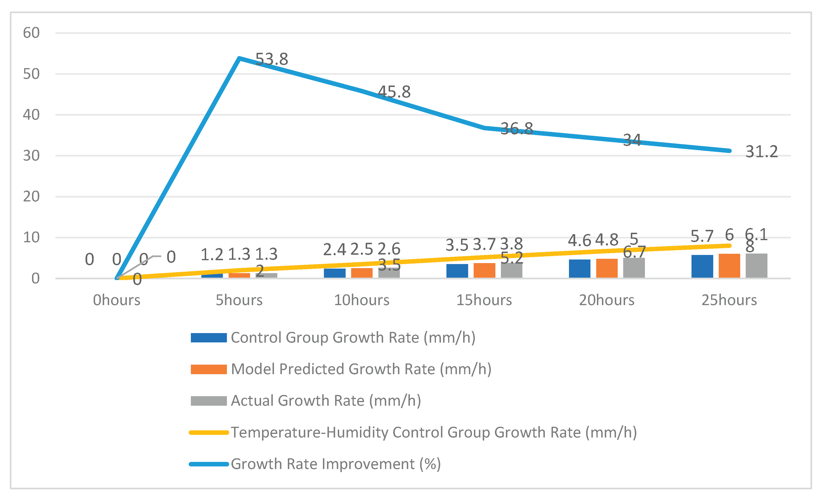
From the table, it is evident that the experimental group with the temperature-humidity coupling control system significantly outperforms the control group in growth rate, and the actual growth rate closely matches the model’s predicted value, validating the control model’s effectiveness and accuracy. The temperature-humidity control strategy demonstrated a significant improvement in growth rate across all experimental stages, indicating that it effectively promotes the growth of edible fungi.
6.4. Control System Dynamic Response Performance and Robustness Analysis
Dynamic response and robustness are evaluated by examining whether the system returns rapidly and smoothly to the target set points under sudden disturbances and model uncertainties. Table 5 shows that after a disturbance (e.g.; changes in external temperature and humidity), the deviations decrease quickly and the system recovers to the stable region within a few minutes, with recovery errors generally less than 0.3 °C and 0.5% RH.
From the data analysis, it can be seen that the system’s recovery time after disturbance is short, and the recovery errors are less than 0.3 °C and 0.5% humidity, demonstrating good dynamic response and robustness.
6.5. System Energy Consumption Analysis and Control Optimization Effect Evaluation
Energy consumption is evaluated by comparing the temperature-control energy, humidity-control energy, and total energy consumption across strategies (Table 6). The no-control case shows a total consumption of 8.6 kWh, while PID reduces it to 6.7 kWh, and fuzzy-PID further reduces it to 5.7 kWh.
With the optimized strategy, the total energy consumption decreases to 4.8 kWh, indicating a substantial improvement in energy efficiency while maintaining regulation performance.
The table shows that the optimized control strategy significantly reduced energy consumption for temperature-humidity regulation. Compared to the no-control strategy, energy efficiency improved by 47.3%.
7. Conclusion and Outlook
7.1. Summary of Research Conclusions
This study addresses the coupled temperature–humidity regulation problem in an edible fungi growth environment and develops a simulation-based control framework integrating a coupled dynamic model and a fuzzy-PID controller. The main conclusions are as follows.
(1) Stable tracking: Under the target set-points (e.g.; 22 °C and 90%RH), the closed-loop system can enter the stable region within minutes and maintain small steady-state fluctuations.
(2) Disturbance rejection: When step disturbances of ±2 °C and ±5%RH are injected, the system suppresses deviations effectively and returns to the target range within a short recovery time (about several minutes in the tested cases).
(3) Growth improvement: Compared with the no-regulation control group, the temperature–humidity regulated group achieves a clear growth-rate advantage. The growth-rate improvement in Table 4 ranges from 31.2% to 53.8% across the simulated period, averaging approximately 40%, and the measured growth rate is close to the model-predicted value, supporting model consistency.
(4) Energy saving: Energy-consumption comparison shows that the optimized strategy reduces total energy consumption (e.g.; from 8.6 kWh to 4.8 kWh) and achieves an energy-efficiency improvement of 47.3% in Table 6, indicating better cost-effectiveness while maintaining regulation performance.
7.2. Application Value of the Model and Control Strategy
The proposed coupled model and control strategy provide a reusable reference for environmental regulation in edible fungi cultivation. From an engineering perspective, the method offers a practical way to coordinate temperature and relative humidity, supporting stable environmental maintenance under external variations and reducing regulation-induced fluctuations.
Beyond edible fungi rooms, the same modeling-and-control idea can be extended to other controlled-environment agriculture scenarios (e.g.; greenhouse cultivation and plant factories). With appropriate parameter re-identification and set-point redesign for different crops or growth stages, the framework can serve as a baseline solution for smart-agriculture environmental control and energy-efficient operation.
7.3. Future Research Directions
Future work will focus on transferring the simulation framework to practical deployments and improving model generalization across species and cultivation stages. First, model parameters and growth-response functions should be re-identified for different edible fungi varieties and growth phases so that set-points and control constraints match real production requirements.
Second, advanced data-driven methods (e.g.; reinforcement learning for parameter self-tuning, or deep models for disturbance prediction) can be introduced on top of the PID/fuzzy-PID baseline to enhance adaptivity under highly variable environments. Finally, integrating low-cost sensors, actuator dynamics, and IoT-based monitoring will enable closed-loop validation in real cultivation rooms and support remote supervision and energy-aware control.
Future work will incorporate explicit coupling compensation and disturbance estimation to further improve performance under strong external perturbations. Disturbance models and state-estimation mechanisms (e.g.; Kalman-filter-based estimation) can be integrated to compensate system inputs online and enhance robustness in practical deployments .Future work will also include formal stability and controllability analysis of the closed-loop system (e.g.; via linearization and Lyapunov-based approaches) to provide theoretical guarantees in addition to simulation verification.
References
- Chen, Z.; Carter, J.L.; Banwart, A.S.; et al. Environmental levels of microplastics disrupt growth and stress pathways in edible crops via species-specific mechanisms [J]. Frontiers in Plant Science 2025, 16, 1670247–1670247. [Google Scholar] [CrossRef] [PubMed]
- Nora, A.; Hutabarat, C.J. D.; Lioe, N.H.; et al. UHPLC-HRMS-based metabolomics and antioxidant compounds of culinary mushrooms grown in Indonesia [J]. Journal of Food Measurement and Characterization 2025, 19, 1–14. [Google Scholar]
- Gao, J.; Zhang, Z.; Wang, Y. Numerical simulation of the growth environment inside edible fungi growth chambers based on CFD methods [J]. Journal of China Agricultural Machinery and Chemistry 2025, 46, 94–100+107. [Google Scholar]
- Hu, Q. Mechanisms of environmental factors affecting the growth, development, and secondary metabolite accumulation of edible fungi [J]. Industrial Microbiology 2025, 55, 234–236. [Google Scholar]
- Timm, G.T.; Arantes, T.S.M.; Oliveira, D.S.H.E.; et al. Substrate effects on the growth, yield, and nutritional composition of edible mushrooms [J]. Advances in Applied Microbiology 2025, 130, 159–190. [Google Scholar] [PubMed]
- Omer, N.S.; Shanmugam, V. Exploring tannery effluent bacteria for bioremediation and plant growth promotion: isolating and characterizing bacterial strains for environmental cleanup [J]. Journal of the Taiwan Institute of Chemical Engineers 2025, 166(P1), 105362–105362. [Google Scholar] [CrossRef]
- Stamford, D.J.; Hofmann, A.T.; Lawson, T. Sinusoidal LED light recipes can improve rocket edible biomass and reduce electricity costs in indoor growth environments [J]. Frontiers in Plant Science 2024, 15, 1447368–1447368. [Google Scholar] [CrossRef] [PubMed]
- Jian, Guan; Wenchao, Shang; Hui, Yan; et al. Electrical automation control strategies during the growth cycle of edible fungi and their impact on yield [J]. Special Economic Animals and Plants 2024, 27, 166–168. [Google Scholar]
- Yuhua, Gong; Jinying, Li; Chunmou, Wei; et al. Establishment of a correlation model between environmental factors and the fruiting body development of Morchella sextelata [C] // Chinese Mycological Society; Proceedings of the 2024 Annual Conference of the Chinese Mycological Society. Institute of Applied Mycology, Huazhong Agricultural University; National Key Laboratory of Agricultural Microbial Resources Discovery and Utilization; Hubei Hongshan Laboratory, 2024; p. 130. [Google Scholar]
- Shunquan, Gao. Research on understory edible mushroom cultivation modes [J]. China Forestry Industry 2024, 62–63. [Google Scholar]
- K. S. A., Sangeeta M. K., T. P. Microgreens of tropical edible-seed species, an economical source of phytonutrients—insights into nutrient content, growth environment, and shelf life [J]. Future Foods 2023, 8.
- Pei, Hong; Lili, Shu; Tianlai, Li; et al. Effects of light environment on the growth and development of edible fungi [J]. Journal of Edible Fungi 2021, 28, 108–115. [Google Scholar]
- Mulan, Hu. Application of computer technology in efficient cultivation and green pest control of edible fungi—Review of Efficient Cultivation and Green Pest Control of Edible Fungi [J]. China Edible Fungi 2020, 39, 284. [Google Scholar]
- Ye, Wei. Discussion on ecological environmental design in pollution-free factory production of edible fungi [J]. China Edible Fungi 2019, 38, 53–55+61. [Google Scholar]
- Ou, Long. Development of agricultural tourism resources—A case study of edible mushroom resources in Guizhou Province [J]. China Edible Fungi 2019, 38, 108–110. [Google Scholar]
- Li, Li; Jinglong, Jiang; Xiaohui, Ji; et al. Overview of minerals and heavy metals in wild edible fungi [J]. Food Industry Technology 2015, 36, 395–400. [Google Scholar]
- Wenke, Liu; Qichang, Yang. Photobiology of edible fungi and progress of LED applications [J]. Science & Technology Review 2013, 31, 73–79. [Google Scholar]
- Man, Lu; Haihui, Zhang; Boyou, Lu; et al. Research on edible fungi growth environment control systems [J]. Agricultural Mechanization Research 2013, 35, 111–114+118. [Google Scholar]
- Hailong, Yu; Qian, Guo; Juan, Yang; et al. Research progress on the effects of environmental factors on the growth and development of edible fungi [J]. Shanghai Agricultural Journal 2009, 25, 100–104. [Google Scholar]
- Chuncheng, Wu; Tianlai, Li; Ningning, Ma. Effects of different compost treatments on major environmental factors of greenhouse soil and the growth and development of tomatoes [J]. China Vegetables 2005, 4–7. [Google Scholar]

Table 1.
Simulation Parameter Design.
| Parameter Name | Value Range | Description |
|---|---|---|
| Temperature Setting Range | 18 °C ~ 28 °C | Temperature adjustment range |
| humidity Setting Range | 80% ~ 95% | humidity adjustment range |
| Air Heat Capacity | 1.0 J/(kg·K) | Simulated air heat capacity |
| Evaporation Rate | 0.05 kg/s | Evaporation rate for humidity control |
| External Temperature-humidity Disturbance | ±2 °C, ±5% RH | Range of external temperature-humidity disturbances |
Table 2.
Steady-State Control Performance Experiment Data.
| Time (min) | External temperature (°C) | External humidity (%) | Target Temperature (°C) | Target humidity (%) | Actual Temperature (°C) | Actual humidity (%) | Temperature Deviation (°C) | humidity Deviation (%) | Steady-State Time (min) |
|---|---|---|---|---|---|---|---|---|---|
| 0 | 25 | 80 | 22 | 90 | 22.5 | 89 | 0.5 | -1 | 5 |
| 10 | 24.8 | 82 | 22 | 90 | 22.2 | 89.5 | 0.2 | -0.5 | 5 |
| 20 | 25.2 | 79 | 22 | 90 | 22.1 | 89.8 | 0.1 | -0.2 | 5 |
| 30 | 24.9 | 81 | 22 | 90 | 22.1 | 89.9 | 0.1 | -0.1 | 5 |
| 40 | 25 | 80 | 22 | 90 | 22 | 90 | 0 | 0 | 5 |
Table 3.
Disturbance Suppression Ability Experiment Data.
| Time (min) | External Temperature Disturbance (°C) | External humidity Disturbance (%) | Target Temperature (°C) | Target humidity (%) | Actual Temperature (°C) | Actual humidity (%) | Temperature Deviation (°C) | humidity Deviation (%) | Recovery Time (min) |
|---|---|---|---|---|---|---|---|---|---|
| 0 | 0 | 0 | 22 | 90 | 22 | 90 | 0 | 0 | 0 |
| 5 | 2 | 5 | 22 | 90 | 24 | 95 | 2 | 5 | - |
| 10 | 2 | 5 | 22 | 90 | 23.5 | 94 | 1.5 | 4 | - |
| 15 | 2 | 5 | 22 | 90 | 22.3 | 91.5 | 0.3 | 1.5 | 2 |
| 20 | 2 | 5 | 22 | 90 | 22.1 | 90.5 | 0.1 | 0.5 | 5 |
| 25 | 0 | 0 | 22 | 90 | 22 | 90 | 0 | 0 | 5 |
Table 4.
Growth Rate Improvement and Model Validation Experiment Data.
| Time (hours) | Control Group Growth Rate (mm/h) | Model Predicted Growth Rate (mm/h) | Actual Growth Rate (mm/h) | Temperature-humidity Control Group Growth Rate (mm/h) | Growth Rate Improvement (%) |
|---|---|---|---|---|---|
| 0 | 0 | 0 | 0 | 0 | 0 |
| 5 | 1.2 | 1.3 | 1.3 | 2 | 53.8 |
| 10 | 2.4 | 2.5 | 2.6 | 3.5 | 45.8 |
| 15 | 3.5 | 3.7 | 3.8 | 5.2 | 36.8 |
| 20 | 4.6 | 4.8 | 5 | 6.7 | 34 |
| 25 | 5.7 | 6 | 6.1 | 8 | 31.2 |
Table 5.
Control System Dynamic Response Performance and Robustness Experiment Data.
| Time (min) | External Temperature Disturbance (°C) | External humidity Disturbance (%) | Actual Temperature (°C) | Actual humidity (%) | Temperature Deviation (°C) | humidity Deviation (%) | Recovery Time (min) | Recovery Error (°C/% RH) |
|---|---|---|---|---|---|---|---|---|
| 0 | 0 | 0 | 22 | 90 | 0 | 0 | 0 | 0 |
| 5 | 3 | 6 | 25 | 96 | 3 | 6 | 5 | 0.3/0.5 |
| 10 | 3 | 6 | 23.5 | 93 | 1.5 | 3 | 5 | 0.1/0.2 |
| 15 | 3 | 6 | 22.2 | 90.5 | 0.2 | 0.5 | 5 | 0.0/0.1 |
| 20 | 0 | 0 | 22 | 90 | 0 | 0 | 5 | 0 |
Table 6.
System Energy Consumption Analysis and Control Optimization Effect Evaluation Experiment Data.
Table 6.
System Energy Consumption Analysis and Control Optimization Effect Evaluation Experiment Data.
| Control Strategy | Temperature Control Energy Consumption (kWh) | humidity Control Energy Consumption (kWh) | Total Energy Consumption (kWh) | Pre-Optimization Total Energy Consumption (kWh) | Energy Efficiency Improvement (%) |
|---|---|---|---|---|---|
| No Control Strategy | 5.4 | 3.2 | 8.6 | - | - |
| PID Control Strategy | 4.1 | 2.6 | 6.7 | 9.1 | 26.4 |
| Fuzzy-PID Control Strategy | 3.5 | 2.2 | 5.7 | 9.1 | 37.4 |
Disclaimer/Publisher’s Note: The statements, opinions and data contained in all publications are solely those of the individual author(s) and contributor(s) and not of MDPI and/or the editor(s). MDPI and/or the editor(s) disclaim responsibility for any injury to people or property resulting from any ideas, methods, instructions or products referred to in the content. |
© 2026 by the authors. Licensee MDPI, Basel, Switzerland. This article is an open access article distributed under the terms and conditions of the Creative Commons Attribution (CC BY) license.
Copyright: This open access article is published under a Creative Commons CC BY 4.0 license, which permit the free download, distribution, and reuse, provided that the author and preprint are cited in any reuse.


