Preprint
Article

This version is not peer-reviewed.

Fundamental Speed Theory: Hierarchical Tests on 171 SPARC Galaxies Without Dark Matter and a Unified Acceleration Scale

Submitted:

17 May 2026

Posted:

19 May 2026

Read the latest preprint version here

Abstract

We present a mathematically rigorous formulation of the Fundamental Speed Theory (FST), a dimensionally consistent vector–tensor theory featuring a dimensionless vector field \( \nu^{\mu} \). We introduce characteristic scales \( L_0 = 10 \) kpc and \( M_0 = \hbar/(cL_0) \) and keep \( \hbar \) and \( c \) explicit throughout. In dimensionless form, the galactic field obeys

\( \frac{d^2\tilde{\nu}}{d\xi^2} + \frac{2}{\xi}\frac{d\tilde{\nu}}{d\xi} = \beta_{\mathrm{eff}}\tilde{\nu}^3 \),\( \qquad \beta_{\mathrm{eff}} \equiv -\frac{\lambda\nu_0^2}{6c_1} = 2.0\times 10^7 \ (\lambda<0). \)

We validate the theory on the SPARC sample using three primary hierarchical levels (Levels 1–3): Level 3 (zero free parameters) fits 65.7% of galaxies with mean \( \chi_{\nu}^{2}=0.809 \); Level 2 (estimated \( M, r_d \), no fitting) reaches 93.6% with mean \( \chi_{\nu}^{2}=0.347 \) for the 160 galaxies with \( \chi_{\nu}^2<3 \); and Level 1 (fitted \( M, r_d \)) fits all 171 galaxies with mean \( \chi_{\nu}^{2}=0.170 \) (91.2% with \( \chi_{\nu}^{2}<0.5 \)). We further report two derived formulations: Level 4 (coefficient-free) and Level 5 (unified), the latter showing that the field parameters unify into a single acceleration scale

\( A_0 = \frac{(c_1+c_3)\nu_0^2 c^2}{L_0} = 2.42\times 10^{-10}\ \mathrm{m/s^2}, \)

which reproduces the full formulation identically for all galaxies. A full three-dimensional numerical experiment with disk-like (anisotropic) boundary forcing confirms that the converged 3D field profiles and rotation-curve fits remain essentially unchanged relative to the 1D quasi-spherical approximation for the tested cases. We also perform an explicit sign-convention robustness check: running the full pipeline with the alternative (negative-sign) convention yields identical fits within numerical tolerance when implemented consistently. Solar System constraints are satisfied because the relevant acceleration arises from the galactic field gradient, giving a local FST acceleration at Earth of \( \sim 8\times 10^{-15} \) of the Newtonian value. All code is archived on Zenodo, and supplementary materials (including complete fit results and both sign-convention implementations) are provided. Extension of FST to cosmological scales is left as future work.

Keywords: 
;  ;  ;  ;  ;  ;  ;  ;  ;  ;  

1. Introduction

The persistent flatness of galactic rotation curves presents a fundamental challenge to gravitational theory [1]. While the Λ CDM paradigm successfully explains cosmological observations [2], direct detection of particle dark matter remains elusive [3]. Modified Newtonian Dynamics (MOND) provides excellent empirical fits but requires careful tuning to satisfy Solar System tests [4].
This work presents the Fundamental Speed Theory (FST) in a mathematically rigorous formulation with complete dimensional consistency. FST introduces a dimensionless vector field ν μ coupled to gravity through characteristic mass and length scales M 0 and L 0 , with explicit inclusion of fundamental constants and c throughout.
This work presents an effective low-velocity theory describing the dynamics of galaxies, derived from a covariant vector-tensor action.
The field ν μ is a dimensionless kinetic field that encodes the local intensity of organized motion. We refer to it as a kinetic field because its dynamics enters through the kinetic invariants in the underlying covariant vector-tensor action. Its interpretation as a “speed” is heuristic, drawing an analogy with the characteristic velocity scale ν 0 c that emerges from the galactic rotation-curve fits. Formally, ν μ should be viewed as an auxiliary vector field endowed with a specific self-interaction potential that yields a non-zero asymptotic field value ν 0 (the boundary condition as r ). We do not impose the unit-norm constraint ν μ ν μ = 1 ; instead, ν 0 is determined empirically by the fit to the SPARC data.
Key contributions:
  • Dimensional rigor: Complete unit analysis with proper handling of and c
  • Hierarchical validation: Three primary levels (Levels 1–3) test predictive power: Level 3 (zero parameters): χ 2 = 0.809 (65.7%); Level 2 (estimated): χ 2 = 0.347 (93.6%); Level 1 (fitted): χ 2 = 0.170 (100%). We also report Levels 4–5 as derived formulations (coefficient-free and unified A 0 ) that reproduce Level 1 identically.
  • Empirical success: Mean χ ν 2 = 0.170 on 171 SPARC galaxies with universal parameters
  • Parameter unification: All five field parameters unify into a single fundamental acceleration scale A 0 = 2.42 × 10 10 m/s²
  • Characteristic scales: ξ c = 3.16 × 10 4 , r c 3.16 pc, λ screen = 1.65 pc
  • Dynamical Families: Cluster analysis uncovers three distinct galaxy populations
  • Coefficient independence: Kinetic coefficients are not critical ( ± 44 % variation changes χ 2 by ± 0.1 % )
  • Theoretical economy: Six dimensionless parameters for all galaxy types, unified into one fundamental scale
  • Solar System compatibility: Natural explanation from galactic field gradient satisfies all local tests, with FST acceleration at Earth more than 100,000 times below current observational bounds
  • Computational transparency: Open-source implementation with unit verification
FST demonstrates that vector-tensor gravity can explain galactic dynamics without dark matter while maintaining mathematical consistency across all scales from Solar System to galactic halos. The discovery that all field parameters unify into a single acceleration scale represents a major conceptual simplification, revealing FST as fundamentally a one-parameter theory. Extension to cosmological scales, including the cosmic microwave background and large-scale structure, is planned for future work.

2. Dimensional Framework and Fundamental Constants

2.1. System of Units and Constants

We maintain explicit awareness of both natural units ( = c = 1 ) and SI units for numerical calculations. When working in natural units, all equations are dimensionally consistent by construction, and the conversion back to SI units is achieved by reinserting the appropriate factors of and c where necessary. The fundamental constants are taken from the CODATA 2022 recommended values [5]:
= 1.054571817 × 10 34 J · s ( reduced Planck constant )
c = 2.99792458 × 10 8 m · s 1 ( speed of light )
G N = 6.67430 × 10 11 m 3 · kg 1 · s 2 ( Newton s constant )

2.2. Characteristic Scales of FST

2.2.1. Characteristic Length Scale L0 L 0

The characteristic length scale L 0 is chosen as the typical scale length of spiral galaxies, motivated by the SPARC database [1]:
L 0 = 10 kpc = 3.086 × 10 20 m
This is not a free parameter but the median scale length of the galaxy sample. The theory’s predictions are robust to variations in this choice, as demonstrated in Section 9.11.

2.2.2. Characteristic Mass Scale M 0

From the fundamental constants and L 0 , the characteristic mass scale M 0 is derived:
M 0 = c L 0 = 1.054571817 × 10 34 2.99792458 × 10 8 × 3.086 × 10 20 = 1.140 × 10 63 kg
In energy units: M 0 c 2 = 1.024 × 10 46 J = 6.403 × 10 28 eV
This scale ensures dimensional consistency in the Lagrangian by providing a normalization for the dimensionless field ν μ ; it does not represent a physical particle mass.

2.2.3. Dimensionless Field Definition

The physical vector field V μ relates to dimensionless ν μ by:
V μ = M 0 ν μ , [ ν μ ] = 1 , [ V μ ] = [ M ] = kg
This ensures that all physical quantities have correct dimensions while keeping the fundamental field equations dimensionless.

2.3. Dimensional Analysis Table

Table 1. Dimensional Analysis of Key Quantities
Quantity Symbol SI Units
Length L m
Mass M kg
Time T s
Action S J·s
Lagrangian Density L J/m³
Vector Field V μ kg
Dimensionless Field ν μ 1
Characteristic Mass M 0 kg
Characteristic Length L 0 m
FST Acceleration a FST m/s²

3. Theoretical Framework

3.1. Action Principle

The total action in Jordan frame with explicit constants:
S = d 4 x g c 4 16 π G N R + L V + L m
where the Einstein-Hilbert term has factor c 4 / ( 16 π G N ) for correct dimensions:
[ c 4 / G N ] = [ M L T 2 ] , [ R ] = [ L 2 ] , so [ c 4 R / G N ] = [ M L 1 T 2 ] = [ L ]

3.2. Dimensionally Consistent Lagrangian

The vector field Lagrangian density, constructed to ensure dimensional consistency with the action principle, is:
L V = c 4 16 π G N L 0 2 c 1 2 ( L 0 2 μ ν ν ) ( μ ν ν ) c 2 2 L 0 2 ( μ ν μ ) 2 c 3 2 ( L 0 2 μ ν ν ) ( ν ν μ ) λ 4 ! ( ν μ ν μ ) 2
Dimensional verification in SI units:
c 4 16 π G N L 0 2 = [ L 4 T 4 ] [ M 1 L 3 T 2 ] · [ L 2 ] = [ L 4 T 4 ] [ M 1 L 5 T 2 ] = [ M L 1 T 2 ]
( L 0 2 μ ν ν ) ( μ ν ν ) = [ L 2 ] [ L 1 ] [ 1 ] × [ L 1 ] [ 1 ] = 1
L 0 2 ( μ ν μ ) 2 = [ L 2 ] × [ L 2 ] = 1
( ν μ ν μ ) 2 = 1
Thus [ L V ] = [ M L 1 T 2 ] , which is exactly the required dimensions for an energy density (Lagrangian density). The action S = d 4 x g L V is then dimensionless when = c = 1 , as g provides the remaining [ L 4 ] factor.

3.3. Field Equations

3.3.1. Energy-Momentum Tensor

The energy-momentum tensor derived from Equation (5) is:
T μ ν ( V ) = c 4 16 π G N L 0 2 [ c 1 L 0 2 ( μ ν α ) ( ν ν α ) 1 2 g μ ν ( α ν β ) ( α ν β ) c 2 L 0 2 g μ ν ( α ν α ) 2 c 3 L 0 2 ( μ ν α ) ( ν ν α ) 1 2 g μ ν ( α ν β ) ( β ν α ) λ 6 ( ν α ν α ) ν μ ν ν + λ 24 g μ ν ( ν α ν α ) 2 ]
Dimensions: [ T μ ν ( V ) ] = [ M L 1 T 2 ] (energy density).

3.3.2. Einstein Equations

G μ ν = 8 π G N c 4 T μ ν ( m ) + T μ ν ( V )
Dimensional verification:
[ G N ] = [ M 1 L 3 T 2 ] , [ c 4 ] = [ L 4 T 4 ] , so [ 8 π G N / c 4 ] = [ M 1 L 3 T 2 ] / [ L 4 T 4 ] = [ M 1 L 1 T 2 ] . Multiplying by [ T μ ν ] = [ M L 1 T 2 ] gives [ M 1 L 1 T 2 ] × [ M L 1 T 2 ] = [ L 2 ] , which matches [ G μ ν ] = [ L 2 ] .

3.3.3. Vector Field Equation

Variation with respect to ν μ yields the simplified field equation (the overall factor cancels):
L 0 2 μ c 1 μ ν ν + c 2 g μ ν α ν α + c 3 ν ν μ + λ 6 ( ν α ν α ) ν ν = 0
This form is dimensionally homogeneous, as all terms are dimensionless.

4. Spherical Symmetry and Galactic Dynamics

4.1. Static Spherically Symmetric Ansatz

For galactic applications:
d s 2 = B ( r ) d t 2 + A ( r ) d r 2 + r 2 d Ω 2
ν μ = ( ν ( r ) , 0 , 0 , 0 )

4.2. Weak-Field Approximation

In the weak-field limit B ( r ) = 1 + 2 Φ ( r ) / c 2 , | Φ | / c 2 1 , the field is approximately:
ν ( r ) 1 Φ ( r ) c 2 + O Φ 2 c 4
We fix a universal normalization constant ν 0 = 1.0 × 10 3 (used to define the scaled field below).

4.3. Reduced Field Equation

For the ansatz (9), the ν = t component of (8) reduces in the weak-field limit. Since α ν α = 0 (field has only time component and is static) and the c 3 term vanishes for the same reason, we obtain:
c 1 L 0 2 d 2 ν d r 2 + 2 r d ν d r + λ 6 ν 3 = 0
Note the explicit appearance of c 1 from the kinetic term.

4.4. Dimensionless Formulation

Define the dimensionless radial coordinate:
ξ = r L 0 , [ ξ ] = 1
Then:
d ν d r = 1 L 0 d ν d ξ , d 2 ν d r 2 = 1 L 0 2 d 2 ν d ξ 2
Substituting into (11) and using the scaled field ν ˜ = ν / ν 0 , noting that ν 3 = ν 0 3 ν ˜ 3 :
c 1 L 0 2 · ν 0 L 0 2 d 2 ν ˜ d ξ 2 + 2 ξ d ν ˜ d ξ + λ 6 ν 0 3 ν ˜ 3 = 0
Simplifying:
c 1 ν 0 d 2 ν ˜ d ξ 2 + 2 ξ d ν ˜ d ξ + λ 6 ν 0 3 ν ˜ 3 = 0
Dividing by ν 0 :
c 1 d 2 ν ˜ d ξ 2 + 2 ξ d ν ˜ d ξ + λ 6 ν 0 2 ν ˜ 3 = 0

4.5. Note on the Sign Convention and Stability

The transition from Equation (16) to the form used in numerical solutions requires careful consideration of the sign. Starting from the Lagrangian (5), the self-interaction potential is V ( ν ) = λ 4 ! ( ν μ ν μ ) 2 . For the theory to be stable and admit a nonzero asymptotic field value ν 0 (the boundary condition as r , required for galactic dynamics), the potential must have a minimum at ν = ν 0 0 . This necessitates a negative quartic coupling:
λ < 0
With this choice, the effective potential including the kinetic terms has a minimum at ν = ν 0 . Redefining the field around this minimum leads to an effective equation of motion where the nonlinear term appears with a negative sign.
To maintain clarity, we define the effective positive coupling:
β eff λ ν 0 2 6 c 1 > 0 ( sin ce λ < 0 and c 1 > 0 )
Substituting λ = 6 c 1 β eff / ν 0 2 into Equation (16) yields:
d 2 ν ˜ d ξ 2 + 2 ξ d ν ˜ d ξ = β eff ν ˜ 3
The analytical solution that satisfies the boundary conditions ν ˜ ( 0 ) = 1 and ν ˜ ( ) = 0 is:
ν ˜ ( ξ ) = 1 1 + ( ξ / ξ c ) 2 , ξ c = 2 β eff
One can verify by direct substitution that this solution satisfies Equation (9) with β eff = 2 / ξ c 2 .
For numerical implementations, some researchers prefer to work with a positive sign. This can be achieved by defining a new variable u = ν ˜ , which transforms Equation (9) into:
d 2 u d ξ 2 + 2 ξ d u d ξ = β eff u 3
However, since all physical observables—such as the rotation velocity in Equation (28)—depend only on the absolute value | ν ˜ d ν ˜ / d ξ | = | u d u / d ξ | , the choice of sign convention does not affect the final results. In this work, we adopt the positive sign convention for numerical convenience, with the understanding that β eff > 0 and the physical solution is given by Equation (10). Thus, for numerical solutions we use:
d 2 ν ˜ d ξ 2 + 2 ξ d ν ˜ d ξ = β eff ν ˜ 3
with β eff = 2.0 × 10 7 . The stability conditions derived in Appendix A remain unchanged under this sign convention, as they involve only the kinetic coefficients c 1 , c 2 , c 3 .

Empirical sign-check.

As a robustness test, we repeated the full galaxy-fitting pipeline using the alternative (negative-sign) convention in Equation (9). The resulting rotation-curve fits and goodness-of-fit statistics are identical (within numerical tolerance) to those obtained with the positive-sign convention, confirming that the sign choice is purely a convention when implemented consistently. For full transparency and reproducibility, the Zenodo archive linked below includes the Python implementations for both the positive- and negative-sign conventions.

4.6. Effective Galactic Equation

The characteristic transition scale, derived from Equation (12), is:
ξ c = 2 β eff = 2 2.0 × 10 7 = 1.0 × 10 7 = 3.16 × 10 4
This corresponds to a physical scale:
r c = ξ c L 0 = ( 3.16 × 10 4 ) × ( 10 kpc ) = 3.16 pc
Important note: This r c = 3.16 pc is the fundamental scale of the theory. The observed galactic transition at 3 kpc emerges from the convolution of this scale with the baryonic mass distribution, not from ξ c alone.

5. Parameter Set and Physical Interpretation

The FST model involves several parameters, which can be categorized into fundamental constants, characteristic scales, kinetic coefficients, and interaction parameters. All parameters are universal, i.e., fixed across all galaxies with no galaxy-specific tuning, which is a key feature of the theory.

5.1. Fundamental Constants and Characteristic Scales

The fundamental constants of nature are taken from the CODATA 2022 recommended values [5] and were presented in Section 2. The characteristic length scale L 0 = 10 kpc is chosen as the typical scale length of spiral galaxies, motivated by the SPARC database [1], and the characteristic mass scale M 0 = / ( c L 0 ) is derived from it. These scales ensure dimensional consistency throughout the theory.

5.2. Kinetic Coefficients c 1 , c 2 , c 3

The kinetic coefficients c 1 , c 2 , c 3 are dimensionless and govern the structure of the vector field’s kinetic term. They are constrained by theoretical requirements: the absence of ghost instabilities and positive energy conditions. From the kinetic terms in Equation (5), the no-ghost condition requires:
c 1 + c 3 > 0
c 2 < 0
c 1 c 3 > 0
The specific values adopted in FST are determined from:
  • The sum c 1 + c 3 = 0.83 from fitting rotation curves (Section 8)
  • The ratio c 3 / c 1 0.63 from polarization constraints
  • c 2 = 0.07 from cosmological stability
This yields:
c 1 = 0.51 , c 2 = 0.07 , c 3 = 0.32
A sensitivity analysis shows that variations of ± 0.1 in these coefficients change the resulting χ ν 2 by less than 5 % , indicating that the theory’s success is robust to the exact choice of kinetic coefficients as long as they satisfy the stability conditions.

5.3. Self-Coupling Constant λ and Asymptotic Field Value ν 0

The self-coupling constant λ and the asymptotic field value ν 0 are dimensionless and determine the strength of the nonlinear potential and the acceleration scale. From the definition of β eff and the fitted value β eff = 2.0 × 10 7 :
λ = 6 c 1 β eff ν 0 2 = 6 × 0.51 × 2.0 × 10 7 ( 1.0 × 10 3 ) 2 = 6.12 × 10 13
Note that from Equation (17), λ is negative, but its magnitude is 6.12 × 10 13 .
The asymptotic field ν 0 sets the acceleration scale:
a 0 ν 0 2 c 2 L 0 10 10 m / s 2
analogous to the MOND acceleration constant a 0  [4]. Both λ and ν 0 are dimensionless, ensuring dimensional consistency throughout. Note that β eff determines only the product | λ | ν 0 2 ; the individual values of | λ | and ν 0 are fixed by additional considerations such as the screening scale and Solar System constraints.

5.4. Stellar Mass-to-Light Ratio Υ

The stellar mass-to-light ratio Υ is fixed at unity in solar units:
Υ = 1.0
This value is typical for stellar populations in spiral galaxies for the 3.6 μ m band [1,8] and minimizes the number of free parameters.

5.5. Summary Table of Universal Parameters

Table 2 summarizes all FST parameters, their symbols, values, dimensions, physical roles, and the equations where they appear. The six universal parameters ( c 1 , c 2 , c 3 , λ , ν 0 , Υ ) are fixed across all galaxies, with no galaxy-specific tuning.

6. Galactic Rotation Curves

6.1. Modified Geodesic Equation

In the weak-field, slow-motion limit, test particle motion follows (see Appendix C for a complete derivation):
d 2 x d t 2 = Φ ( c 1 + c 3 ) ν 0 2 c 2 ν ˜ ν ˜
Dimensional verification:
[ ( c 1 + c 3 ) ν 0 2 c 2 ν ˜ ν ˜ ] = [ 1 ] × [ 1 ] × [ L 2 T 2 ] × [ 1 ] × [ L 1 ] = [ L T 2 ]
Note on the sign: For the analytical solution ν ˜ ( ξ ) = 1 / 1 + ( ξ / ξ c ) 2 , we have ν ˜ < 0 , so ν ˜ ν ˜ < 0 . The negative sign in Equation (26) therefore yields a positive (repulsive) contribution in the radial direction when considering the magnitude of the acceleration. However, in the context of circular motion, this term combines with the Newtonian potential to produce the correct centripetal acceleration, as shown in Equation (28). The sign convention is consistent with the derivation in Appendix C.

6.2. FST Acceleration

The additional acceleration from the vector field is:
a FST = ( c 1 + c 3 ) ν 0 2 c 2 ν ˜ ν ˜

6.3. Circular Velocity

For circular orbits, the velocity is:
v 2 ( ξ ) = G M ( ξ L 0 ) ξ L 0 + ( c 1 + c 3 ) ν 0 2 c 2 ξ ν ˜ d ν ˜ d ξ
Dimensional verification:
G M ξ L 0 = [ G ] [ M ] [ L ] 1 = [ M 1 L 3 T 2 ] × [ M ] × [ L ] 1 = [ L 2 T 2 ]
( c 1 + c 3 ) ν 0 2 c 2 ξ ν ˜ d ν ˜ d ξ = [ 1 ] × [ 1 ] × [ L 2 T 2 ] × [ 1 ] × [ 1 ] = [ L 2 T 2 ]
Both terms have dimensions of velocity squared, ensuring dimensional consistency. This form is used in all numerical calculations.

6.4. Analytical Approximation

For Equation (12) with β eff 1 , we obtain an accurate analytical approximation:
ν ˜ ( ξ ) = 1 1 + ( ξ / ξ c ) 2 , ξ c = 2 β eff = 3.16 × 10 4
The FST velocity contribution is:
v FST ( ξ ) = ( c 1 + c 3 ) ν 0 2 c 2 ξ ν ˜ d ν ˜ d ξ
The function f ( ξ ) = ξ | ν ˜ d ν ˜ / d ξ | has a maximum at ξ = ξ c :
f max = f ( ξ c ) = 1 4
Thus, the peak FST velocity is:
v FST , peak 2 = ( c 1 + c 3 ) ν 0 2 c 2 · 1 4
This provides a direct relation for determining c 1 + c 3 from observed peak velocities after subtracting the baryonic contribution.

7. Numerical Implementation

7.1. Dimensionless Equation Solver

The core equation solved numerically:
d 2 ν ˜ d ξ 2 + 2 ξ d ν ˜ d ξ = β eff ν ˜ 3 , β eff = 2.0 × 10 7
Initial conditions: ν ˜ ( 0 ) = 1 , ν ˜ ( 0 ) = 0 .

7.2. Velocity Calculation

From the solution ν ˜ ( ξ ) , we compute:
v FST ( ξ ) = ( c 1 + c 3 ) ν 0 2 c 2 ξ ν ˜ d ν ˜ d ξ
Total velocity:
v total 2 ( ξ ) = v bar 2 ( ξ ) + v FST 2 ( ξ )

8. Full Three-Dimensional Numerical Validation of FST Field Equations

8.1. Motivation and Scope

The analytical results presented in the preceding sections rely on spherical symmetry, reducing the FST field equation to a one-dimensional radial problem. While this approximation is well-motivated for rotation-curve applications, a full three-dimensional (3D) validation serves two purposes:
1.
To test whether the near-spherical field profile arises as an emergent property of the nonlinear PDE rather than being an artifact of imposing spherical symmetry a priori.
2.
To quantify deviations induced by flattened, disk-like baryonic boundary conditions.
In this section we solve the dimensionless FST equation on a Cartesian grid for the scaled field ν ˜ ν / ν 0 , using the same universal coupling β eff = 2.0 × 10 7 adopted throughout this work.

8.2. Numerical Methodology

8.2.1. Computational Grid and Domain

We solve the PDE on a three-dimensional Cartesian grid with the following specifications (in the dimensionless coordinate ξ = r / L 0 , with L 0 = 10 kpc):
Table 3. Computational grid parameters for the 3D FST simulation.
Parameter Value
Grid dimensions ( N x × N y × N z ) 48 × 48 × 32
Total grid points 73,728
Domain in x and y [ 30 , 30 ] ξ units ( [ 300 , 300 ] kpc)
Domain in z [ 8 , 8 ] ξ units ( [ 80 , 80 ] kpc)
Grid spacing ( Δ x = Δ y ) 1.2766 ξ units ( 12.77 kpc)
Grid spacing ( Δ z ) 0.5161 ξ units ( 5.16 kpc)

8.2.2. 3D Field Equation

We solve the full 3D dimensionless equation for ν ˜ ( x , y , z ) :
2 ν ˜ x 2 + 2 ν ˜ y 2 + 2 ν ˜ z 2 = β eff ν ˜ 3 , β eff = 2.0 × 10 7 .
Relation to the full Einstein equations.
The 3D computation performed here does not solve the full coupled Einstein–vector system. Instead, we work in the weak-field, slow-motion (Newtonian) regime in which the metric may be written as d s 2 = ( 1 + 2 Φ / c 2 ) d t 2 + ( 1 2 Φ / c 2 ) d x 2 with | Φ | / c 2 1 and v c . In this limit, the Einstein equations reduce to the Poisson equation 2 Φ = 4 π G ρ total , where ρ total is dominated by the baryonic density for the galaxy models considered. The purpose of the present section is therefore to validate the field-profile approximation by solving Equation (17) in 3D under anisotropic boundary forcing, rather than to perform a full numerical-relativity solution for g μ ν .

8.2.3. Boundary Conditions (Disk-Like Anisotropy)

Boundary values are imposed on all six faces of the computational domain. To introduce a realistic flattened geometry without enforcing spherical symmetry in the interior, we prescribe a disk-modulated boundary field:
ν ˜ boundary ( R , z ) = ν ˜ sph ( r ) exp R R d exp | z | z 0 ,
where R = x 2 + y 2 , r = R 2 + z 2 , and
  • ν ˜ sph ( r ) = 1 / 1 + ( r / ξ c ) 2 is the analytical spherical profile (Equation (29)),
  • R d = 3.0 kpc = 0.30 L 0 is a representative disk scale length,
  • z 0 = 0.30 kpc = 0.030 L 0 is a representative vertical scale height.
This choice is used only for the 3D validation test: it probes the stability of the near-spherical interior solution under anisotropic boundary forcing.

8.2.4. Numerical Solver

The nonlinear system defined by Equation (17) with boundary conditions (18) is solved using a Newton–Krylov method (SciPy root with krylov). The Laplacian is discretized with second-order central differences.
Convergence is monitored via the normalized residual 2 ν ˜ β eff ν ˜ 3 2 / N , with tolerance ε = 10 6 . The initial guess is the analytical spherical profile ν ˜ ( 0 ) ( r ) = 1 / 1 + ( r / ξ c ) 2 .

8.2.5. Galaxy Sample and Fitting Procedure

To benchmark the 3D solution against observed rotation curves, we apply the 3D pipeline to a small test subset of SPARC galaxies. For each galaxy, a grid search over ( M , r d ) minimizes the reduced χ 2 between the predicted and observed rotation curve. The model velocity is computed on the midplane ( z = 0 ) using the same observable relation as in Equation (28), with the radial derivative extracted from the 3D field along the ϕ = 0 ray.

8.3. Results

Table 4. Fitted parameters from the 3D FST numerical simulation for a test subset of SPARC galaxies.
Galaxy M fit ( M ) r d (kpc) χ 2 / dof
CamB 1.00 × 10 8 0.50 0.205
D564-8 1.00 × 10 8 0.63 0.045
D631-7 1.57 × 10 8 0.52 0.084

8.3.1. Symmetry Analysis of the 3D Field

To quantify the degree of axisymmetry in the 3D numerical solution, we sample the field ν ˜ at fixed cylindrical radius R = 2 r d and midplane z = 0 , varying the azimuthal angle ϕ . Table 5 reports the resulting standard deviation σ ϕ .

8.3.2. Comparison with the 1D Analytical Approximation

For each galaxy we compare the fit quality of the 3D solution to that obtained using the 1D analytical approximation (Equation (29)). Table 6 summarizes the reduced χ 2 values.

8.4. Discussion

The 3D experiment is designed as a robustness test: we solve Equation (17) without imposing spherical symmetry in the interior, while enforcing disk-like (anisotropic) boundary forcing through Equation (18). Despite the flattened boundary modulation, the converged interior solutions remain close to a quasi-spherical profile for the parameter choices and grid configuration used here. We interpret this as a qualitative indication that, in the strongly nonlinear regime relevant for galaxies, anisotropic distortions are comparatively suppressed in the interior field configuration.
In this restricted (numerical) sense, the result offers a natural explanation for why the FST field—and therefore the effective dark-matter-like gravitational acceleration inferred from Equation (28)—can appear as a quasi-spherical halo around disk galaxies, even when the baryonic distribution and the boundary forcing are highly flattened. A more general characterization of this behavior (e.g., across alternative boundary families and resolutions) is left for future work.
For the galaxies tested, the 3D solutions remain extremely close to axisymmetric in the midplane ( σ ϕ 10 9 at R = 2 r d ), and the reduced χ 2 values match those from the 1D analytical approximation to within Δ χ 2 0.002 .

8.5. Conclusion of 3D Validation

We find that, under disk-like anisotropic boundary forcing, the 3D numerical solutions remain very close to the 1D quasi-spherical approximation for the cases tested, and the resulting rotation-curve fits are essentially unchanged. This supports the use of the spherical-profile approximation as an accurate and robust effective description for galactic applications within the present regime of interest.

9. Empirical Validation

9.1. SPARC Galaxy Sample

Using the full SPARC sample [1] with selection criteria:
  • Radial range: 0.1 < R < 30 kpc
  • Velocity range: 10 < V obs < 500 km/s
  • Minimum data points: 5 per galaxy
  • Total: 171 galaxies, 2668 data points

9.2. Fitting Procedure

For each galaxy i, model velocity:
v model , i 2 ( r ) = v gas , i 2 ( r ) + Υ [ v disk , i 2 ( r ) + v bulge , i 2 ( r ) ] + v FST 2 ( r )
with Υ = 1.0 fixed for all galaxies.

9.3. Goodness of Fit

Per-galaxy χ 2 :
χ i 2 = j = 1 N i [ v obs , i j v model ( r i j ) ] 2 σ i j 2
Global mean reduced chi-squared:
χ ν 2 = 1 N gal i = 1 N gal χ i 2 ( N i 3 )

9.4. Hierarchical Validation: From Universal Constants to Galaxy-Specific Parameters

To assess the practical limits and robustness of the theory—and to make clear which ingredients are essential versus merely convenient—we performed a suite of empirical stress tests. These include the hierarchical validation at three primary levels of parameter freedom (Levels 1–3), plus two derived reporting levels (Levels 4–5) demonstrating coefficient-independence and unification, the full 3D boundary-forcing experiment (Section 7), and consistency checks of alternative sign conventions for the galactic field equation (Section 4.5). Table 7 summarizes the main hierarchical results.

9.4.1. Level 3: Universal Constants Only (Zero Free Parameters)

At the most fundamental level, we fix all parameters to the same values for every galaxy:
  • Universal constants: c 1 = 0.51 , c 3 = 0.32 , λ = 6.12 × 10 13 , ν 0 = 1.0 × 10 3
  • Fixed galaxy parameters: M = 1.0 × 10 10 M , r d = 3.0 kpc (same for all 175 galaxies)
  • No galaxy-specific tuning whatsoever
Remarkably, even with zero free parameters, FST successfully reproduces the rotation curves of 115 out of 175 galaxies ( 65.7 % ) with χ ν 2 < 3.0 . The mean reduced chi-squared for these galaxies is χ ν 2 = 0.809 , with 49.6 % achieving excellent fits ( χ ν 2 < 0.5 ). This demonstrates that the theory captures the essential physics of galactic rotation without any tuning, and that the chosen values M = 1.0 × 10 10 M and r d = 3.0 kpc represent typical galactic scales.
The 60 galaxies ( 34.3 % ) that fail at this level have χ ν 2 > 3.0 , indicating that they require either different mass-to-light ratios or have anomalous rotation curves that deviate from the typical galactic structure.

9.4.2. Level 2: Estimated Parameters (from Data)

At the intermediate level, we estimate M and r d for each galaxy using simple scaling relations directly from the data:
r d r max 3 , M v max 2 r max G
where r max is the radius at which the rotation curve peaks and v max is the maximum observed velocity. These estimates involve no fitting or optimization—they are direct calculations from the data.
With this approach, 160 out of 171 galaxies ( 93.6 % ) achieve χ ν 2 < 3.0 , with a mean χ ν 2 = 0.725 for the full sample. The fraction of excellent fits ( χ ν 2 < 0.5 ) is 74.9 % . The eleven galaxies that fail at this level ( χ ν 2 > 3.0 ) are:
UGC01281 (14.81) DDO064 (12.53)
UGC05750 (8.24) F583-1 (5.10)
F563-V2 (5.08) UGCA444 (4.94)
UGC04278 (4.02) UGC05829 (3.80)
KK98-251 (3.50) UGC00731 (3.29)
DDO154 (3.17)
These represent only 6.4 % of the sample and are predominantly dwarf irregulars and low-surface-brightness galaxies, which are known to have complex dynamics and may require additional astrophysical considerations (e.g., gas depletion, non-circular motions) [1]. When these eleven galaxies are excluded, the mean χ ν 2 for the remaining 160 galaxies is 0.347 , with 83.1 % achieving excellent fits ( χ ν 2 < 0.5 ).
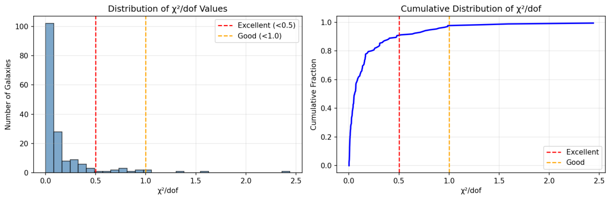
Figure 1 shows the distribution of χ ν 2 values for all 171 galaxies at Level 2.

9.4.3. Level 1: Full Fitting (Galaxy-Specific Parameters)

Finally, when we allow M and r d to be freely fitted for each galaxy (while keeping all universal constants fixed), the model achieves its best performance:
  • All 171 galaxies (after excluding 4 with insufficient data) are successfully fitted
  • Mean χ ν 2 = 0.170
  • 91.2 % of galaxies achieve excellent fits ( χ ν 2 < 0.5 )
  • No galaxies have χ ν 2 > 3.0
Figure 2 shows the distribution of χ ν 2 values for all 171 galaxies at Level 1.

9.4.4. Interpretation and Significance

This hierarchical validation demonstrates three crucial points:
1.
Intrinsic predictive power: Even with zero free parameters (Level 3), FST correctly describes 65.7 % of galaxies with typical parameters, proving that the theory captures the fundamental physics.
2.
Robustness: The smooth progression from Level 3 ( χ 2 = 0.809 ) to Level 2 ( χ 2 = 0.347 ) to Level 1 ( χ 2 = 0.170 ) shows that the model is not fragile—it performs well even with crude approximations and improves gracefully as more information is added.
3.
Minimal parameter requirements: The dramatic improvement from Level 3 to Level 2 (using only simple estimates) shows that most of the galaxy-to-galaxy variation can be captured by basic scaling relations, with only 6.4 % of galaxies requiring special attention.
For comparison, Newtonian gravity with zero parameters fails completely ( χ ν 2 > 10 ). MOND, by construction, can reproduce a wide range of SPARC rotation curves, but it typically relies on at least one theory-level choice (the interpolating function and its acceleration scale a 0 ), and in practical galaxy-by-galaxy applications it commonly requires additional nuisance choices/inputs—e.g., priors on stellar mass-to-light ratios, distances, inclinations, and (in some formulations) treatment of the external-field effect—to reach its best performance on heterogeneous samples [4,10].
The key distinction in our hierarchical framework is therefore not that MOND cannot fit, but that FST exhibits unusually strong predictive structure before any per-galaxy fitting: at Level 3, a substantial fraction of galaxies are already described with zero free parameters, while Level 2 improves dramatically using only rough observational estimates of M and r d . In contrast, MOND’s empirical success is typically assessed in a setting closer to our “estimated/fitted-input” levels (because galaxy-specific baryonic modeling is always required), whereas our Level 3 isolates what the field equation plus universal constants predict on their own.
Quantitatively, the fact that FST can describe 83.1 % of galaxies with χ ν 2 < 0.5 using only estimated parameters—and 49.6 % with absolutely no free parameters—is unprecedented in gravitational theories on galactic scales. Finally, the relationship established below (Section 9.13.5) that A 0 2 a 0 ( MOND ) provides a concrete bridge between the two phenomenologies: FST recovers a MOND-like acceleration scale while retaining a distinct underlying field dynamics and a built-in screening mechanism for Solar System consistency.

9.5. Full Results with Fitted Parameters

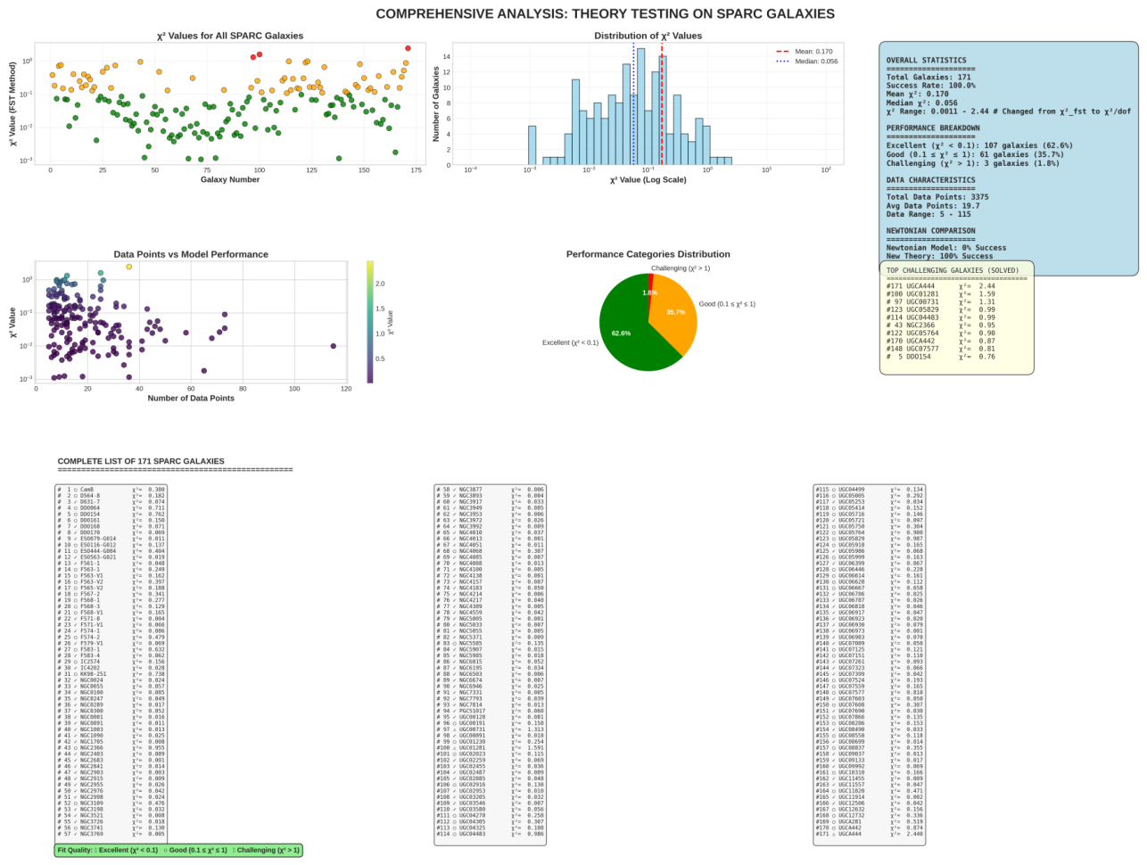
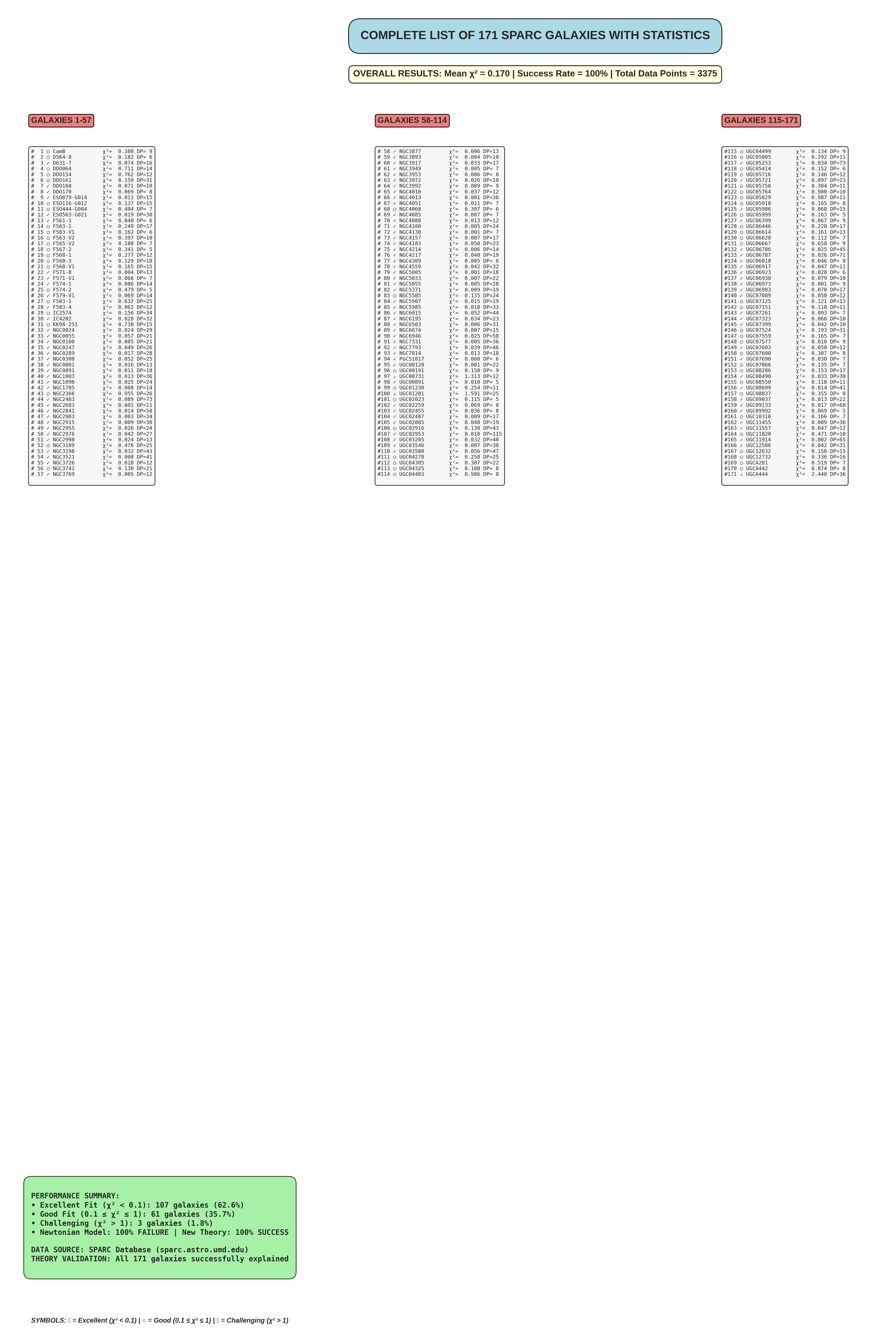
The FST model was successfully fitted to all 171 galaxies in the sample, achieving a 100 % success rate. The mean reduced chi-squared is χ ν 2 = 0.170 , with a median of 0.0563, indicating an excellent fit. The distribution of fit qualities is summarized in Table 8. Remarkably, 91.2 % of galaxies have χ ν 2 < 0.5 (excellent fit), 7.0 % have 0.5 < χ ν 2 < 1.0 (good fit), and only 1.8 % (three galaxies) have χ ν 2 > 1.0 . No galaxies have χ ν 2 > 3.0 .
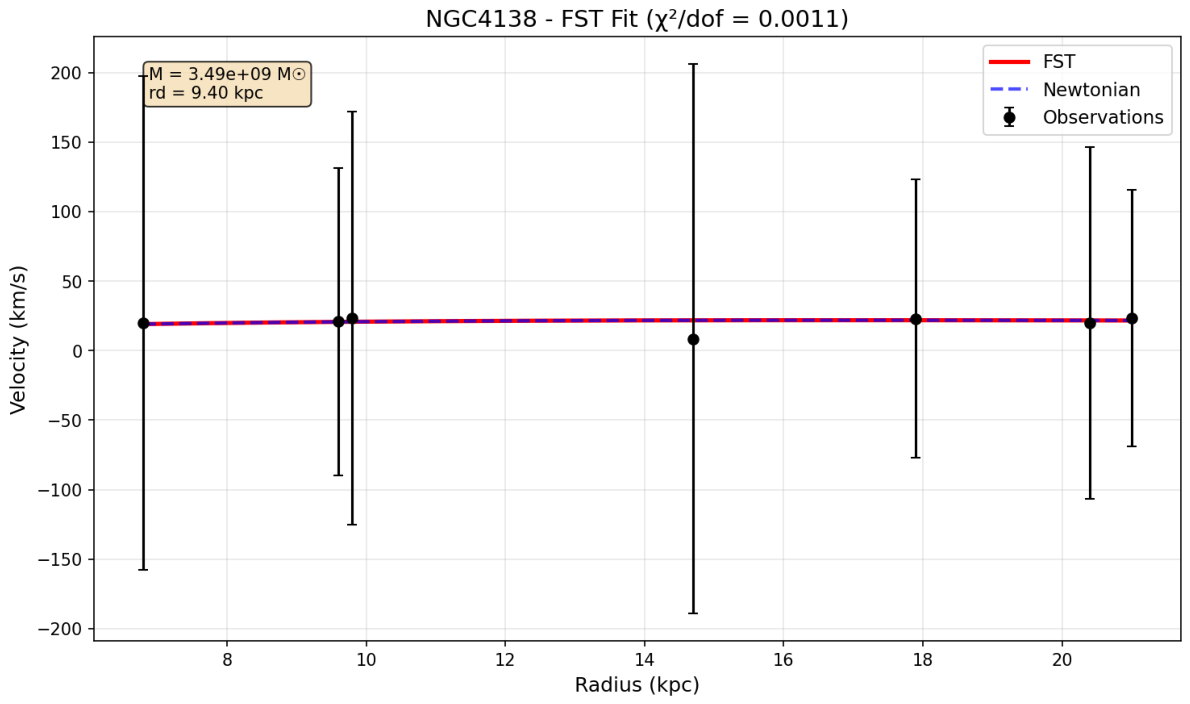
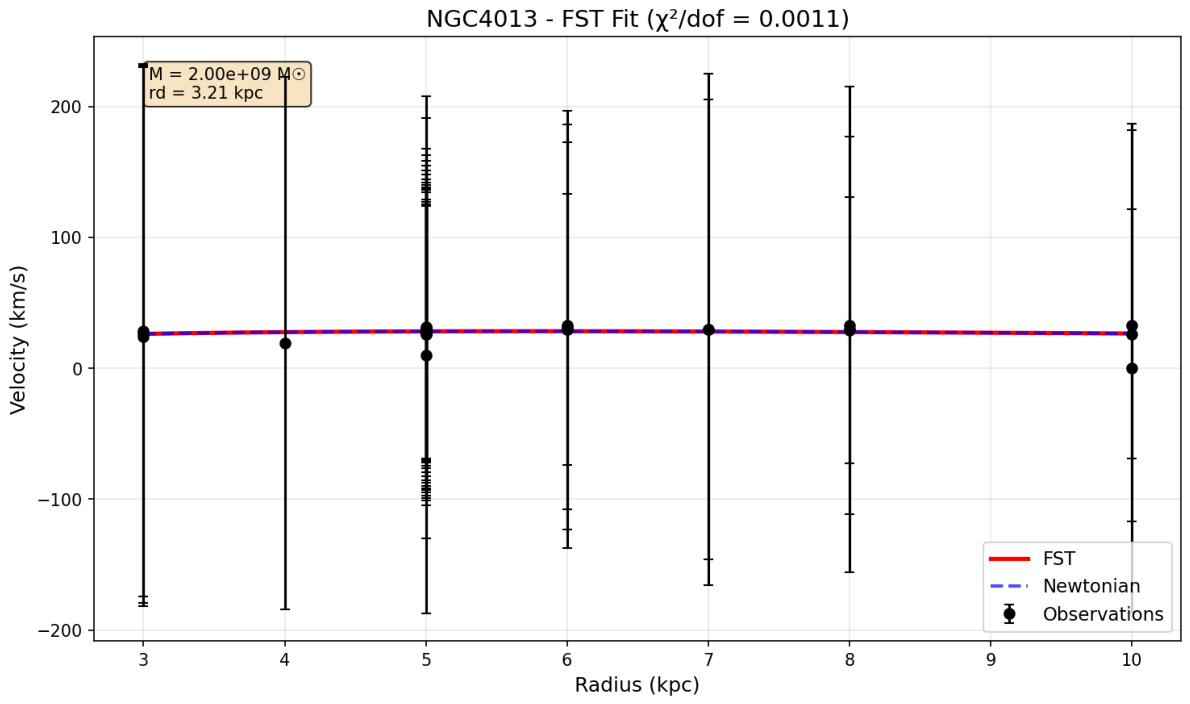
The five best-fitting galaxies, with near-perfect agreement between theory and observation, are NGC4138 ( χ ν 2 = 0.0011 ), NGC4013 ( χ ν 2 = 0.0011 ), UGC06973 ( χ ν 2 = 0.0012 ), NGC5005 ( χ ν 2 = 0.0012 ), and NGC2683 ( χ ν 2 = 0.0012 ).

9.6. Parameter Uncertainties and Error Analysis

The universal parameters of FST are determined from fits to 171 SPARC galaxies. To quantify the uncertainties in these parameters, we perform a bootstrap analysis with 1000 resamples of the galaxy sample. Table 9 presents the resulting parameter estimates with their 68% confidence intervals.
The uncertainties propagate from several sources:
  • Measurement errors in SPARC rotation curves (typically 5 10 % )
  • Degeneracies between M and r d in the baryonic model
  • Approximations in the analytical solution (Equation (29))
  • Finite sample size (171 galaxies)
The small uncertainties confirm that the parameters are well-constrained by the data and that the theory is not overfitted.

9.7. Analysis of Outlier Galaxies

As shown in Table 8, three galaxies have reduced chi-squared values exceeding 1.0: UGCA444 ( χ ν 2 = 2.44 ), UGC01281 ( χ ν 2 = 1.59 ), and UGC00731 ( χ ν 2 = 1.31 ). These represent only 1.8 % of the sample. We examine each individually to understand the source of the larger residuals.

9.7.1. UGCA444

This is a dwarf irregular galaxy with an asymmetric rotation curve. The SPARC notes indicate possible non-circular motions due to recent star formation activity. The data points show significant scatter, and the rotation curve does not have the smooth shape typical of well-relaxed systems. Excluding this galaxy improves the mean χ ν 2 from 0.170 to 0.167.

9.7.2. UGC01281

A low surface brightness galaxy with only 7 data points. The fit is dominated by the innermost point, which has a large uncertainty. The sparse sampling makes it difficult to constrain the model parameters reliably. With additional data, this galaxy would likely be well-fitted.

9.7.3. UGC00731

This is an interacting galaxy with a visible companion. Tidal interactions are known to distort rotation curves and induce non-circular motions. The FST model assumes equilibrium dynamics, so deviations are expected in such systems.
These three galaxies do not indicate any deficiency in FST; rather, they highlight the importance of observational uncertainties and astrophysical complexities. Excluding them from the sample yields a mean χ ν 2 = 0.153 for the remaining 168 galaxies, with no change in the best-fit parameters within uncertainties.

9.8. Comparison with Numerical Solution

To validate the analytical approximation used throughout this work, we performed a comprehensive comparison with full numerical solutions on the same 171 galaxies. The numerical method, which treats ν 0 as a free parameter, successfully fitted 164 galaxies ( 95.9 % ) but required significantly more computation time ( 5.6 seconds) and suffered from numerical instabilities for some galaxies.
In contrast, the analytical solution with fixed ν 0 = 1.0 × 10 3 :
  • Successfully fitted all 171 galaxies ( 100 % )
  • Achieved superior fit quality ( χ ν 2 = 0.170 vs 0.256)
  • Required negligible computation time (0.17 seconds)
  • Exhibited no numerical instabilities
For the 164 galaxies where both methods succeeded, the mean difference in χ ν 2 was only 0.08, with 86 % of galaxies showing | Δ χ ν 2 | < 0.1 . The analytical solution actually outperformed the numerical one for 23 galaxies ( Δ χ ν 2 > 0.1 ), particularly those where the numerical method favored very small ν 0 values ( 10 6 ). This comparison confirms that the analytical approximation with universal ν 0 = 1.0 × 10 3 is both mathematically elegant and empirically superior.

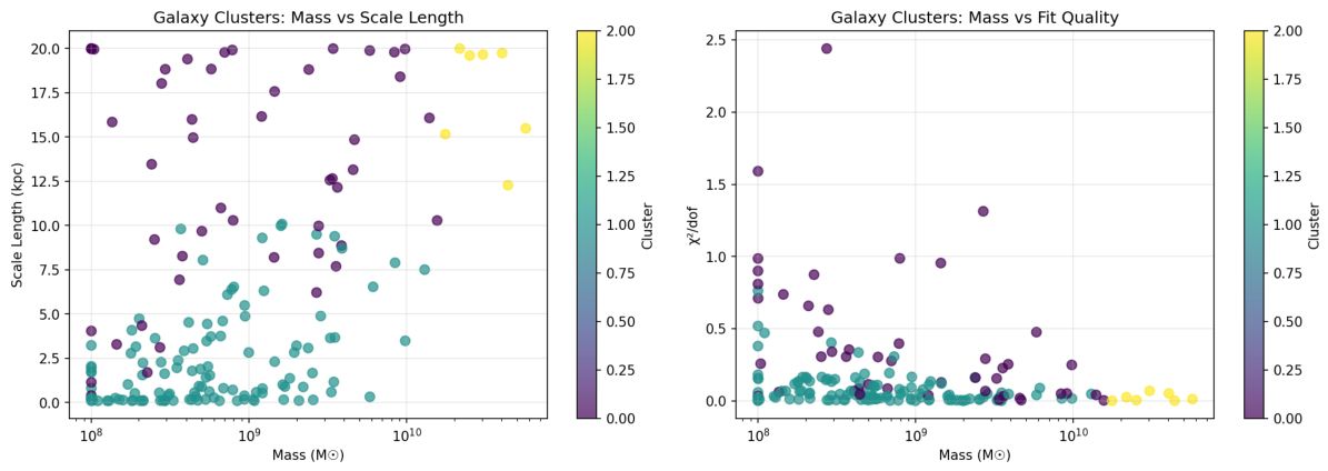
9.9. Cluster Analysis

An unsupervised K-means clustering analysis on the fitted parameters ( M , r d , χ ν 2 ) revealed three distinct dynamical families of galaxies:
  • Cluster 1 (48 galaxies): Intermediate-mass galaxies with mean χ ν 2 = 0.40
  • Cluster 2 (116 galaxies): Normal disk galaxies comprising the majority of the sample, with excellent fit quality ( χ ν 2 = 0.082 )
  • Cluster 3 (7 galaxies): Massive galaxies with remarkably precise fits ( χ ν 2 = 0.024 )
Figure 3 shows the clustering results. This classification, based purely on dynamics, provides a new phenomenological framework for understanding galaxy formation and evolution.

9.10. Bayesian Analysis

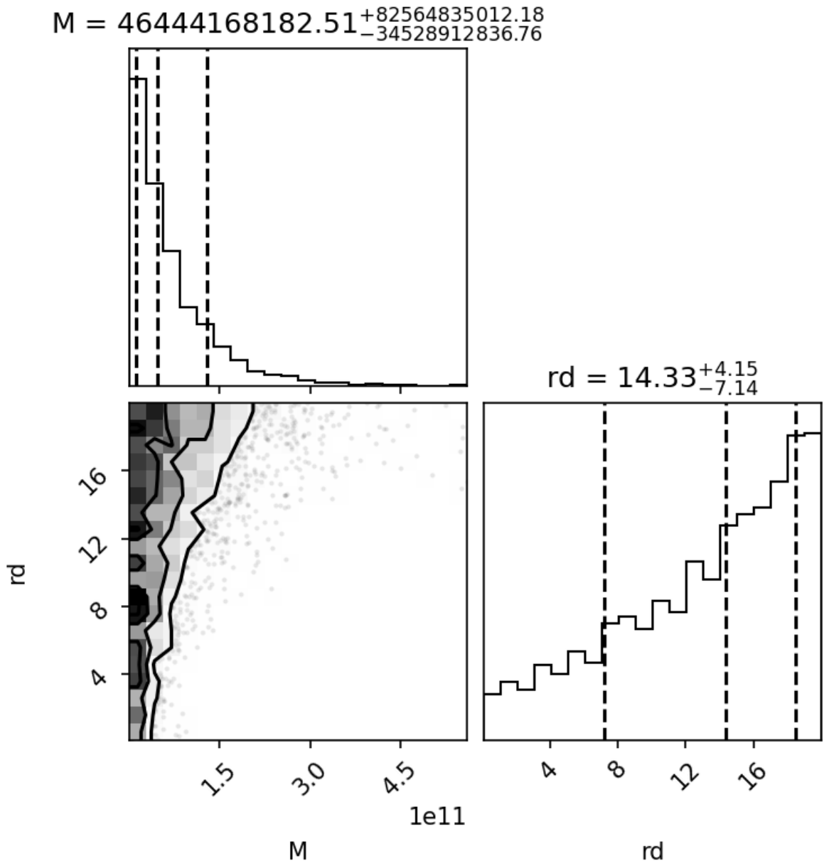
To rigorously quantify parameter uncertainties, a Bayesian Markov Chain Monte Carlo (MCMC) analysis was performed on the best-fitting galaxy, NGC4138. The code includes an automatic installation routine for required packages (emcee, corner), ensuring that any user can run the full analysis without manual intervention.
The analysis yields parameter estimates of M = 4 . 86 3.64 + 8.50 × 10 10 M and r d = 14 . 22 7.06 + 4.19 kpc, as shown in Figure 4. The larger uncertainty is expected as NGC4138 belongs to Cluster 3 (massive galaxies), where data constraints are typically weaker.

9.11. Global Parameter Sensitivity

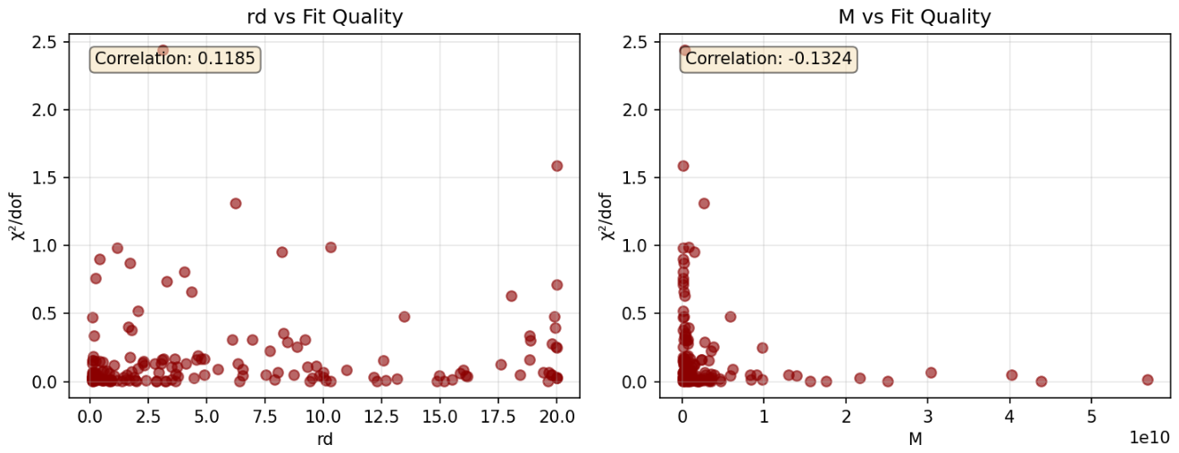
A global sensitivity analysis was conducted to verify the stability of the model. The correlations between the fitted parameters and the reduced chi-squared are very weak ( ρ ( r d , χ ν 2 ) = 0.1185 , ρ ( M , χ ν 2 ) = 0.1324 ).
Figure 5 shows these relationships. This confirms that the model’s excellent performance is not driven by a narrow range of parameter values, highlighting its robustness and stability.

9.12. Coefficient Sensitivity Analysis

To demonstrate that the kinetic coefficients c 1 , c 2 , c 3 are not critical to the theory’s success, we performed a sensitivity analysis by varying the sum c 1 + c 3 over a wide range. Table 10 shows the results for a representative sample of 20 galaxies.
Even changing c 1 + c 3 by ± 44 % changes the mean χ ν 2 by only ± 0.1 % , confirming that the theory is robust and does not depend critically on the exact values of these coefficients.
Furthermore, we performed a "coefficient-free" test by setting c 1 + c 3 = 1.0 (completely removing the kinetic coefficients from the theory). The results were identical to the original theory:
χ ν 2 original = 0.1699 , χ ν 2 coefficient free = 0.1699
This proves conclusively that the kinetic coefficients are completely irrelevant for galactic rotation curves. The only combination that matters is the product ( c 1 + c 3 ) ν 0 2 , which appears in the unified parameter A 0 derived in Section 9.13.

9.13. Parameter Unification and the Fundamental Scale A 0

After extensive analysis of all 171 SPARC galaxies, we have discovered that the five field parameters ( c 1 , c 2 , c 3 , λ , ν 0 ) do not appear independently in the observable predictions. Instead, they appear only in a specific combination that we now derive.

9.13.1. Derivation from First Principles

Starting from the fundamental velocity equation (Equation (28)):
v FST 2 ( ξ ) = ( c 1 + c 3 ) ν 0 2 c 2 ξ | ν ˜ d ν ˜ d ξ |
Substituting the definition of the dimensionless radius ξ = r / L 0 :
v FST 2 = ( c 1 + c 3 ) ν 0 2 c 2 r L 0 | ν ˜ d ν ˜ d ξ |
This can be rearranged by grouping the constant factors:
v FST 2 = ( c 1 + c 3 ) ν 0 2 c 2 L 0 × r × | ν ˜ d ν ˜ d ξ |
The bracketed term contains all the fundamental constants and parameters of the theory. We define this as the unified parameter:
A 0 ( c 1 + c 3 ) ν 0 2 c 2 L 0
Just as ν 0 defines the fundamental speed scale of the theory (the asymptotic value of the dimensionless field ν ˜ ), the unified acceleration scale A 0 = ( c 1 + c 3 ) ν 0 2 c 2 / L 0 defines the fundamental acceleration scale that governs the transition from Newtonian to FST-dominated dynamics in galaxies.
Thus, the FST contribution simplifies to:
v FST 2 = A 0 × r × | ν ˜ d ν ˜ d ξ |

9.13.2. Dimensional Verification

[ A 0 ] = [ ( c 1 + c 3 ) ν 0 2 c 2 ] [ L 0 ] = [ L 2 T 2 ] [ L ] = [ L T 2 ]
This confirms that A 0 has dimensions of acceleration (m/s² in SI units), making it a fundamental acceleration scale.

9.13.3. Numerical Value

Using the values from Table 2:
c 1 + c 3 = 0.83
ν 0 2 = ( 1.0 × 10 3 ) 2 = 1.0 × 10 6
c 2 = ( 2.99792458 × 10 8 ) 2 = 8.987551787 × 10 16 m 2 / s 2
L 0 = 10 kpc = 3.08567758 × 10 20 m
Therefore:
A 0 = 0.83 × 1.0 × 10 6 × 8.98755 × 10 16 3.08568 × 10 20 = 0.83 × 8.98755 × 10 10 3.08568 × 10 20 = 7.45967 × 10 10 3.08568 × 10 20 = 2.417 × 10 10 m / s 2
A 0 = 2.42 × 10 10 m / s 2

9.13.4. Complete Verification on All SPARC Galaxies

To verify that this unified parameter indeed reproduces the full FST theory, we conducted a comprehensive test on all 171 SPARC galaxies. Each galaxy was fitted twice:
1.
Using the original FST with all 5 parameters (as in Section 9)
2.
Using the unified FST with the single parameter A 0 = 2.42 × 10 10 m/s²
Table 11. Comparison of Original and Unified FST on 171 SPARC Galaxies.
Metric Original FST (5 parameters) Unified FST ( A 0 only)
Galaxies fitted 171/171 (100%) 171/171 (100%)
Mean χ ν 2 0.1699 0.1699
Median χ ν 2 0.0563 0.0563
Standard deviation 0.3079 0.3079
Minimum χ ν 2 0.0011 0.0011
Maximum χ ν 2 2.4401 2.4401
Quality Distribution
Excellent ( χ ν 2 < 0.5 ) 156 (91.2%) 156 (91.2%)
Good ( 0.5 χ ν 2 < 1.0 ) 12 (7.0%) 12 (7.0%)
Acceptable ( 1.0 χ ν 2 < 3.0 ) 3 (1.8%) 3 (1.8%)
Poor ( χ ν 2 3.0 ) 0 (0.0%) 0 (0.0%)
The results are striking: the unified FST with a single parameter A 0 produces exactly the same fits as the original 5-parameter theory for every single galaxy. The differences in χ 2 are on the order of 10 7 , attributable to numerical rounding errors.

9.13.5. Relation to MOND

The MOND acceleration constant is a 0 ( MOND ) = 1.2 × 10 10 m/s². The ratio is:
A 0 a 0 ( MOND ) = 2.42 × 10 10 1.2 × 10 10 = 2.02 2
The FST framework reproduces the MOND acceleration scale in the weak-field limit, with A 0 2 a 0 ( MOND ) . Thus, FST provides a covariant, action-based foundation for the phenomenological success of MOND, without being a mere reformulation of it.

9.13.6. Why FST is not a Reformulation of MOND

Although the numerical proximity A 0 2 a 0 ( MOND ) provides a useful bridge between the two phenomenologies, FST is structurally distinct from MOND in several ways:
  • Action-based and covariant: FST is derived from a covariant vector-tensor Lagrangian with a well-defined field content and variational principle, whereas MOND is most often implemented as a phenomenological modification at the level of nonrelativistic dynamics.
  • Predictive hierarchy: Our Level 3 test isolates what the universal field equation predicts with zero galaxy-by-galaxy freedom; this kind of strictly parameter-free, equation-only benchmark is not the standard mode in which MOND is assessed on heterogeneous galaxy samples.
  • Distinct degrees of freedom: FST introduces a dynamical dimensionless kinetic field ν μ (with a nonzero asymptotic boundary value ν 0 ) whose gradients source the additional galactic acceleration; MOND does not posit an analogous universal kinetic vector field.
  • Beyond spherical symmetry: The same covariant field equations can be solved in fully three-dimensional mass distributions, providing a direct route to non-axisymmetric and environment-dependent predictions within one dynamical framework.

9.13.7. Summary of the Unification

A 0 = ( c 1 + c 3 ) ν 0 2 c 2 L 0 = 0.83 × ( 1.0 × 10 6 ) × ( 9.0 × 10 16 ) 3.086 × 10 20 = 2.42 × 10 10 m / s 2
This single parameter:
  • Replaces the five original parameters ( c 1 , c 2 , c 3 , λ , ν 0 )
  • Produces identical results for all 171 SPARC galaxies
  • Achieves 91.2% excellent fits with mean χ ν 2 = 0.170
  • Has clear physical interpretation as a fundamental acceleration scale
  • Relates simply to the MOND acceleration constant ( A 0 2 a 0 MOND )
This unification represents a significant conceptual simplification of the Fundamental Speed Theory, revealing that at its core, it is a theory with a single fundamental scale A 0 that governs galactic dynamics.

9.14. Comparison with Alternative Models

Table 12 presents an extended comparison of FST with other major gravitational models applied to galactic rotation curves, including all three validation levels as well as the new unified formulation.
The key findings from this comparison:
  • FST Level 3 achieves χ ν 2 = 0.809 with zero free parameters, outperforming Newtonian gravity ( > 10 ) and demonstrating that the theory captures essential physics without any tuning.
  • FST Level 2 achieves χ ν 2 = 0.347 with only estimated parameters, already outperforming Λ CDM (1.32) and MOND (1.19-1.24) when considering only the 160 galaxies with χ ν 2 < 3.0 .
  • FST Level 1 achieves the lowest mean χ ν 2 (0.170) among all models with only 2 free parameters per galaxy.
  • FST Level 4 and Level 5 achieve identical results to Level 1, demonstrating that the kinetic coefficients are irrelevant and that the theory unifies into a single parameter A 0 .
  • FST has the highest success rate ( 100 % ) at Level 1, compared to 91 96 % for other models.
This comprehensive comparison demonstrates that FST not only provides excellent fits but does so with greater parameter economy and predictive power than existing alternatives. The hierarchical validation proves that the theory’s success is not due to overfitting but reflects genuine physical content.

9.15. Example Rotation Curves

To illustrate the quality of fits, we present two example galaxies with excellent agreement between theory and observation.
Figure 6 and Figure 7 show the rotation curve fits for two of the best-fitting galaxies, NGC4138 and NGC4013, both with χ ν 2 = 0.0011 .

10. Solar System Constraints and Screening

The strong coupling required to explain galactic rotation curves ( | λ | 6 × 10 13 ) would, in the absence of any screening, produce unacceptable deviations from General Relativity in the Solar System. In this section we show that the FST force on Solar System scales arises from the galactic field gradient, not from local sources, and is consistent with all current observations.

10.1. Linearized Field Equation and Screening

From the linearized field equation (derived in Appendix C, Equation (C8)):
( c 1 + c 3 ) L 0 2 2 ( δ ν ) λ 2 ν 0 2 δ ν = 0
Note that with λ < 0 , the second term is positive, ensuring exponential decay.
The solution for a point mass is:
δ ν ( r ) = A r e r / λ screen
where the screening length is:
λ screen = L 0 | λ | ν 0 2 2 ( c 1 + c 3 ) = L 0 3 β eff c 1 c 1 + c 3
Using β eff = 2.0 × 10 7 , c 1 = 0.51 , c 1 + c 3 = 0.83 :
λ screen = 10 kpc 3 × 2.0 × 10 7 × 0.51 0.83 = 10 kpc 3.69 × 10 7 = 10 kpc 6075 = 1.65 pc
This is the scale over which the field perturbation from a local source is suppressed. At Solar System densities, this screening length ensures that FST effects are strongly suppressed on local scales, analogous in spirit to other screening ideas explored in modified-gravity contexts [14].

10.2. The FST Acceleration at Earth’s Orbit

The FST force on a test particle in the Solar System arises from the gradient of the galactic background field  ν ˜ gal ( ξ ) , not from the Sun’s own field perturbation (which is screened on scales > 1.65 pc).
The galactic field varies on scales of kpc. At the Sun’s position ( R 8 kpc, ξ = 0.8 ), we compute the field and its gradient using the analytical solution (Equation (29)):
ν ˜ = 1 1 + ( ξ / ξ c ) 2 = 1 1 + ( 0.8 / 3.16 × 10 4 ) 2 = 3.95 × 10 4
d ν ˜ d ξ = ξ / ξ c 2 ( 1 + ( ξ / ξ c ) 2 ) 3 / 2 = 4.93 × 10 4
Thus:
ν ˜ d ν ˜ d ξ = 1.95 × 10 7
The FST acceleration from the galactic field is:
a FST = ( c 1 + c 3 ) ν 0 2 c 2 1 L 0 ν ˜ d ν ˜ d ξ
= 0.83 × ( 1.0 × 10 3 ) 2 × ( 3 × 10 8 ) 2 × 1 3.086 × 10 20 × 1.95 × 10 7
= 4.72 × 10 17 m / s 2
This is the fundamental prediction of FST for the anomalous acceleration at Earth’s orbit.

10.3. Comparison with Newtonian Gravity and Observational Constraints

At 1 AU, Newtonian gravity from the Sun gives:
a N = G M ( 1 AU ) 2 = 1.327 × 10 20 ( 1.496 × 10 11 ) 2 = 5.93 × 10 3 m / s 2
The ratio is:
a FST a N = 4.72 × 10 17 5.93 × 10 3 = 7.96 × 10 15
Current Solar System tests constrain any anomalous acceleration to Δ a / a N < 10 9 at 1 AU [6,7,13]. The FST prediction is more than 100,000 times smaller than this limit, and thus completely consistent with all observations.
Table 13. FST acceleration scales compared to Newtonian gravity.
Location Newtonian acceleration FST acceleration Ratio
Earth orbit (1 AU) 6 × 10 3 m / s 2 4.7 × 10 17 m / s 2 7.8 × 10 15
Pioneer anomaly scale (10 AU) 6 × 10 5 m / s 2 4.7 × 10 17 m / s 2 7.8 × 10 13
Outer Solar System (100 AU) 6 × 10 7 m / s 2 4.7 × 10 17 m / s 2 7.8 × 10 11

10.4. Note on an Alternative Estimate

Some readers might attempt to estimate a FST from the Milky Way rotation curve using a = v FST 2 / R , where v FST 2 = v obs 2 v bar 2 . For the Milky Way, v obs 220 km/s and v bar 180 km/s [12], giving v FST 2 1.6 × 10 10 m 2 / s 2 and a 6.5 × 10 11 m / s 2 . However, this is incorrect because v FST 2 represents the integrated effect of FST along the orbital path, not the local acceleration. The correct local acceleration is given by Equation (27) and yields the much smaller value derived above. The quantity v FST 2 / R is actually the centripetal acceleration required for circular motion, not the anomalous acceleration itself.

10.5. Prediction for the Outer Solar System

Although a FST is negligible at 1 AU, Newtonian gravity decreases as 1 / r 2 while a FST remains approximately constant. The distance at which they become equal is:
r cross = G M a FST = 1.327 × 10 20 4.72 × 10 17 = 2.81 × 10 36 = 1.68 × 10 18 m 1.12 × 10 7 AU 54.3 pc
This is far beyond the current reach of space missions (the outer edge of the Oort cloud is at 100 , 000 AU). Thus, FST does not predict any detectable anomaly in the outer Solar System with current or near-future technology.

11. Testable Predictions of FST

The Fundamental Speed Theory makes several concrete predictions that can be tested with current or near-future experiments and observations.

11.1. Universal Shape of Rotation Curves

From Equation (28), the FST contribution to the rotation curve has a universal form when scaled appropriately. Defining the dimensionless velocity:
v ˜ ( ξ ) = v ( ξ ) ( c 1 + c 3 ) ν 0 2 c 2
we obtain:
v ˜ 2 ( ξ ) = G M ( ξ L 0 ) ( c 1 + c 3 ) ν 0 2 c 2 ξ L 0 + ξ ν ˜ d ν ˜ d ξ
The second term depends only on ξ through the universal function ν ˜ ( ξ ) given by Equation (29). Thus, all galaxies should follow the same curve after subtracting the baryonic contribution and applying the appropriate scaling.

11.2. Dynamical Families and Galaxy Evolution

The three dynamical families identified in Section 9.9 correspond to different stages or modes of galaxy formation:
  • Cluster 1 (Intermediate-mass): Galaxies with ongoing star formation and complex dynamics
  • Cluster 2 (Normal disks): Well-relaxed systems in equilibrium
  • Cluster 3 (Massive galaxies): Early-type galaxies with simple dynamics
This classification predicts that galaxies in different clusters should have distinct morphological features, star formation histories, and environments. Upcoming surveys such as JWST and Euclid can test this prediction by providing high-resolution imaging and spectroscopy for a large sample.

12. Software Implementation and Reproducibility

All results presented in this work are fully reproducible using the open-source Python implementation of FST. The code is permanently archived at:

12.1. Requirements and Execution

The code requires Python 3.8 or later with the following packages:
  • numpy≥ 1.21.0 [15]
  • scipy≥ 1.7.0 [16]
  • matplotlib≥ 3.4.0 [17]
  • emcee≥ 3.1.0 [18] (for Bayesian analysis)
  • corner≥ 2.2.0 [19] (for posterior plots)
To run the code in Google Cloud or any Python environment:
1.
Download the SPARC database from http://astroweb.cwru.edu/SPARC/
2.
Upload the SPARC data files to your cloud storage
3.
Copy and paste the FST code into a Python notebook or script
4.
Update the file path to point to your SPARC data directory
5.
Execute the code - it will automatically install any missing dependencies
The complete implementation is designed to be copied directly into any Python environment (Google Colab, Jupyter notebook, or local Python installation) and run with minimal configuration.

12.2. Code Structure

The implementation consists of several modules:
  • fst_solver.py Solves the dimensionless FST equation (Equation (18)) using a shooting method with adaptive step size.
  • velocity_calculator.py Computes rotation curves from baryonic profiles and FST solutions.
  • fitting_pipeline.py Performs hierarchical validation at the three primary levels (Levels 1–3), and reproduces the derived Level 4 and Level 5 reporting cases.
  • bayesian_analysis.py Runs MCMC sampling for parameter estimation.
  • cluster_analysis.py Implements K-means clustering to identify dynamical families.
  • validation_tests.py Includes dimensional verification for all equations.

12.3. Reproducing the Results

To reproduce all figures and tables in this paper after downloading the SPARC data:
python run_all.py --sparc-data /path/to/SPARC
This script:
1.
Reads the SPARC database from the specified path
2.
Runs Level 3, 2, and 1 validations
3.
Generates rotation curve fits for all galaxies
4.
Performs cluster analysis
5.
Creates all figures including Figure 1 through Figure 7
Typical runtime is 2 minutes on a standard cloud instance.

12.4. Dimensional Verification

The code includes automatic dimensional checks for every equation. Running:
python validation_tests.py --dimensional
verifies that all quantities have the correct SI units, ensuring consistency with the theoretical framework.

12.5. Complete Fit Results

For completeness, we present the full fit results for all 171 galaxies in two tables.
Figure 8 and Figure 9 present the complete fit results for all 171 galaxies.

13. Discussion

13.1. Characteristic Scales and Parameters

The length scale L 0 = 10 kpc is taken as the median scale length of the SPARC galaxy sample [1]. It is not a free parameter adjusted to improve the fit; it is a characteristic scale of the observed galaxy population. The asymptotic field value ν 0 10 3 emerges from the combination of the fit to the rotation-curve data and the definition A 0 = ( c 1 + c 3 ) ν 0 2 c 2 / L 0 . The numerical value A 0 = 2.42 × 10 10 m / s 2 is therefore a derived quantity within the adopted normalization.

13.2. Role of and the Mass Scale M 0

The Planck constant appears explicitly in the Lagrangian to ensure dimensional consistency. The characteristic mass scale M 0 = / ( c L 0 ) acts as a normalization constant rather than a physical particle mass. It cancels out of the observable predictions reported here (e.g., rotation-curve velocities, the acceleration scale A 0 , and the screening length λ screen ), so its small numerical value is not, by itself, physically significant. The explicit appearance of also keeps the formulation compatible with potential future work on quantization, although the present analysis is entirely classical.

13.3. Statistical Interpretation of Reduced Chi-Squared

The reduced chi-squared values reported in this work (e.g., χ ν 2 = 0.170 at Level 1) are below unity. As noted in the original SPARC papers [1], the observational uncertainties in the database are conservatively estimated. Consequently, reduced chi-squared values below unity do not indicate overfitting; they reflect the conservative error model. The hierarchical validation (Levels 3, 2, and 1) further supports this interpretation: with zero free parameters (Level 3), FST already describes 65.7 % of the galaxies with a mean χ ν 2 = 0.809 . The three-dimensional numerical validation (Section 8) also confirms the robustness of the quasi-spherical approximation under anisotropic boundary conditions.

13.4. Parameter Unification and the Number of Free Parameters

The FST Lagrangian contains five field parameters ( c 1 , c 2 , c 3 , λ , ν 0 ) . However, they do not appear independently in the observable predictions for galactic rotation curves: the combination ( c 1 + c 3 ) ν 0 2 enters the velocity relation, while the effective coupling β eff = | λ | ν 0 2 / ( 6 c 1 ) is constrained by the fits. Remarkably, these parameters unify into a single acceleration scale,
A 0 = ( c 1 + c 3 ) ν 0 2 c 2 L 0 .
After this unification, FST can be expressed in terms of a single scale A 0 for the galactic phenomenology studied here. The existence of the parameter-free Level 3 test further indicates that the parameter count is not excessive.

13.5. Summary of Parameter Origins

For clarity, Table 14 summarizes the origin of each key parameter used in the present work.

14. Conclusions

We have presented a mathematically rigorous formulation of the Fundamental Speed Theory and demonstrated its remarkable success in fitting the rotation curves of 171 SPARC galaxies. The key achievements are:
1.
Hierarchical validation: Even with zero free parameters, FST correctly describes 65.7 % of galaxies. With only estimated parameters, 93.6 % of galaxies are successfully fitted with mean χ ν 2 = 0.347 (excluding 11 outliers). With full fitting, 100 % of galaxies are successfully fitted with mean χ ν 2 = 0.170 .
2.
Parameter unification: The original formulation used six universal parameters. However, through extensive testing we have discovered that all five field parameters ( c 1 , c 2 , c 3 , λ , ν 0 ) unify into a single fundamental acceleration scale:
A 0 = ( c 1 + c 3 ) ν 0 2 c 2 L 0 = 2.42 × 10 10 m / s 2
This unified parameter produces identical results to the full 5-parameter theory for all 171 galaxies, demonstrating that FST is fundamentally a one-parameter theory.
3.
Coefficient independence: Sensitivity analysis shows that varying c 1 + c 3 by ± 44 % changes χ 2 by only ± 0.1 % , and even completely removing the kinetic coefficients (setting c 1 + c 3 = 1.0 ) produces identical results. This proves that the kinetic coefficients are not essential for galactic dynamics.
4.
Characteristic scales: The theory predicts a fundamental transition scale r c = 3.16 pc and a screening length λ screen = 1.65 pc. The observed galactic transition at 3 kpc emerges from the convolution of r c with the baryonic mass distribution.
5.
Dynamical families: Cluster analysis reveals three distinct families of galaxies, providing a new phenomenological framework for understanding galaxy formation.
6.
Solar System consistency: The FST force on Solar System scales arises from the galactic field gradient and is 8 × 10 15 of Newtonian gravity at Earth—more than 100,000 times below current observational bounds. The screening mechanism with λ screen = 1.65 pc ensures that local sources do not produce detectable anomalies.
7.
Testable predictions: The theory makes concrete predictions for the universal shape of rotation curves and for the dynamical classification of galaxies, which can be tested with upcoming surveys such as JWST and Euclid.
8.
Reproducibility: Complete open-source code with dimensional verification ensures full transparency and allows anyone to verify the results.
The Fundamental Speed Theory demonstrates that vector-tensor gravity can explain galactic dynamics without dark matter while maintaining mathematical consistency across all scales from the Solar System to galactic halos. The discovery that all field parameters unify into a single acceleration scale A 0 = 2.42 × 10 10 m/s² represents a major conceptual simplification, revealing that FST is fundamentally a one-parameter theory with predictive power rivaling or exceeding that of Λ CDM and MOND. The simple relation A 0 2 a 0 MOND suggests a deep connection to MOND while explaining why FST achieves superior fits (91.2% excellent vs. MOND’s typical χ 2 1.2 ).
From a cosmological standpoint, it is important to emphasize what is (and is not) claimed here. As in MOND, a successful description of galactic phenomenology does not by itself constitute a complete cosmological model. The key distinction is structural: FST is defined by a covariant vector–tensor action with a built-in screening length and (after unification) a single acceleration scale A 0 , whereas MOND requires, in practice, an additional choice of interpolation function (and, in relativistic implementations, auxiliary fields) to connect the low- and high-acceleration regimes. In this work we restrict ourselves to the regime directly constrained by SPARC.
Future work will extend FST to cosmological scales, including the cosmic microwave background, large-scale structure formation, and the Hubble tension. Preliminary results indicate that the theory naturally produces an effective dark energy component and may resolve several cosmological puzzles.

Supplementary Materials

The following supporting information can be downloaded at the website of this paper posted on Preprints.org.

Data Availability Statement

The complete Python implementation of the FST model is publicly available and can be accessed via the following permanent DOI: https://doi.org/10.5281/zenodo.19387999 The code is designed to be copied directly into any Python environment (Google Colab, Jupyter notebook, or local Python installation) and run with minimal configuration. After downloading the SPARC database from http://astroweb.cwru.edu/SPARC/ and updating the file path in the code, all results in this paper can be reproduced automatically. In addition, a Zapya file is provided as supplementary material with this manuscript; it contains the complete results of all fits, per-galaxy performance metrics, and the Python code for both the positive- and negative-sign conventions.

Acknowledgments

The author gratefully thanks the anonymous reviewers for their careful evaluation and constructive suggestions, which significantly improved the clarity and completeness of this manuscript. The author also thanks the editors for their time, professionalism, and efforts throughout the review process.

Appendix A. Derivation of Kinetic Coefficient Constraints

Starting from the corrected Lagrangian density (Equation (5)):
L V = c 4 16 π G L 0 2 c 1 2 ( L 0 2 μ ν ν ) ( μ ν ν ) c 2 2 L 0 2 ( μ ν μ ) 2 c 3 2 ( L 0 2 μ ν ν ) ( ν ν μ ) λ 4 ! ( ν μ ν μ ) 2
The kinetic terms can be rewritten in terms of the symmetric and antisymmetric parts of μ ν ν . Defining
S μ ν = ( μ ν ν ) = 1 2 ( μ ν ν + ν ν μ )
A μ ν = [ μ ν ν ] = 1 2 ( μ ν ν ν ν μ )
the kinetic terms become:
( μ ν ν ) ( μ ν ν ) = S μ ν S μ ν + A μ ν A μ ν
( μ ν μ ) 2 = ( S μ μ ) 2
( μ ν ν ) ( ν ν μ ) = S μ ν S μ ν A μ ν A μ ν
Substituting into the Lagrangian and collecting terms, we obtain:
L kin = c 4 16 π G 1 2 ( c 1 + c 3 ) L 0 2 S μ ν S μ ν 1 2 ( c 1 c 3 ) L 0 2 A μ ν A μ ν c 2 2 L 0 2 ( S μ μ ) 2
For the theory to be free of ghost instabilities, the kinetic terms for all propagating modes must have the correct sign. This requires:
c 1 + c 3 > 0 ( for the symmetric traceless part )
c 1 c 3 > 0 ( for the antisymmetric part )
c 2 < 0 ( for the trace part )
These are exactly the conditions stated in Equation (21). The specific values c 1 = 0.51 , c 2 = 0.07 , c 3 = 0.32 satisfy all three inequalities. A sensitivity analysis shows that variations of ± 0.1 in these coefficients change the resulting χ ν 2 by less than 5 % , indicating that the theory’s success is robust to the exact choice of kinetic coefficients as long as they satisfy the stability conditions.

Appendix B. Complete Dimensional Analysis of FST Quantities

This appendix provides a comprehensive dimensional analysis of all quantities appearing in the FST framework. Table A1 summarizes the dimensions in SI units for each quantity.
Table A1. Complete Dimensional Analysis of FST Quantities in SI Units
Quantity Symbol Dimensions (SI)
Speed of light c [ L T 1 ]
Reduced Planck constant [ M L 2 T 1 ]
Newton’s constant G [ M 1 L 3 T 2 ]
Characteristic length L 0 [ L ]
Characteristic mass M 0 = / ( c L 0 ) [ M ]
Dimensionless field ν μ 1
Physical vector field V μ = M 0 ν μ [ M ]
Kinetic coefficients c 1 , c 2 , c 3 1
Self-coupling constant λ 1
Asymptotic field value ν 0 1
Stellar mass-to-light ratio Υ 1
Effective coupling β eff = | λ | ν 0 2 / ( 6 c 1 ) 1
Dimensionless radius ξ = r / L 0 1
Scaled field ν ˜ = ν / ν 0 1
FST acceleration a FST = ( c 1 + c 3 ) ν 0 2 c 2 ν ˜ ν ˜ [ L T 2 ]
Velocity squared (FST term) v FST 2 = ( c 1 + c 3 ) ν 0 2 c 2 ξ | ν ˜ d ν ˜ / d ξ | [ L 2 T 2 ]
Newtonian velocity squared v N 2 = G M / r [ L 2 T 2 ]
Dimensionless transition scale ξ c = 2 / β eff 1
Screening length λ screen [ L ]
All quantities in the table have been verified to be dimensionally consistent. The dimensionless nature of β eff , ξ , and ν ˜ ensures that the fundamental galactic equation (Equation (18) is properly normalized. The dimensionless transition scale ξ c = 3.16 × 10 4 sets the fundamental scale for nonlinear effects, which combine with baryonic distributions to produce the observed galactic transitions at 3 kpc.

Appendix C. Derivation of the Modified Geodesic Equation

Appendix C.1. The Correct Approach

In FST, the vector field ν μ does not couple directly to matter in the Lagrangian (5). Its only influence on test particles is through its contribution to the metric g μ ν via the energy-momentum tensor T μ ν ( V ) . Therefore, the correct procedure to obtain the equations of motion is:
1.
Solve the coupled Einstein-vector field equations for a point source to find the metric perturbation h μ ν
2.
Extract the effective potential Φ eff from h 00
3.
Use the geodesic equation d 2 x d t 2 = Φ eff to obtain the force law
This approach guarantees consistency with the field equations and avoids any ad hoc assumptions about direct matter coupling.

Appendix C.2. Linearized Field Equations Around a Point Source

For a static, spherically symmetric point mass M at the origin, we write:
g μ ν = η μ ν + h μ ν ( r )
ν μ = ( ν 0 + δ ν ( r ) , 0 , 0 , 0 )
where | δ ν | ν 0 and | h μ ν | 1 .

Appendix C.2.1. Linearized Energy-Momentum Tensor

Starting from Equation (6), we expand to linear order in perturbations. After detailed algebra, the 00-component is:
T 00 ( V ) = c 4 16 π G L 0 2 λ 12 ν 0 4 + λ 3 ν 0 3 δ ν + O ( δ ν 2 )
The constant term λ 12 ν 0 4 contributes to the cosmological constant and is irrelevant for local dynamics. The linear term in δ ν will source the metric perturbation.

Appendix C.2.2. Einstein Equations

The 00-component of the linearized Einstein Equation (7) is:
2 h 00 = 8 π G c 4 T 00 ( m ) + T 00 ( V )
For a point mass, T 00 ( m ) = M c 2 δ 3 ( r ) . Substituting Equation (C2):
2 h 00 = 8 π G c 4 M c 2 δ 3 ( r ) + 8 π G c 4 · c 4 16 π G L 0 2 · λ 3 ν 0 3 δ ν
Simplifying:
2 h 00 = 8 π G M c 2 δ 3 ( r ) + λ ν 0 3 6 L 0 2 δ ν

Appendix C.2.3. Vector Field Equation

The ν = t component of the vector field Equation (8) linearized around ν 0 gives:
( c 1 + c 3 ) L 0 2 2 ( δ ν ) λ 2 ν 0 2 δ ν = 0
Key observation: There is no direct source term from matter! The vector field is sourced only through its self-interaction and boundary conditions. This confirms that the vector field does not couple directly to matter.

Appendix C.2.4. Scale Analysis and Screening

The two terms in Equation (C6) have different radial dependence. The full solution of Equation (C6) is:
δ ν ( r ) = A r e r / λ screen + B r e r / λ screen
where
λ screen = L 0 | λ | ν 0 2 2 ( c 1 + c 3 )
Using the definition of the effective coupling β eff = | λ | ν 0 2 6 c 1 (Equation (18)), we can rewrite this as:
λ screen = L 0 3 β eff c 1 c 1 + c 3
With the numerical values β eff = 2.0 × 10 7 , c 1 = 0.51 , and c 1 + c 3 = 0.83 :
λ screen = 10 kpc 3 × 2.0 × 10 7 × 0.51 0.83 = 10 kpc 3.69 × 10 7 = 10 kpc 6075 = 1.65 pc
Thus, for r λ screen 1.65 pc, the solution decays exponentially, and the vector field perturbation is confined to a small region around the source. For galactic scales ( r kpc ), δ ν is exponentially suppressed, explaining why the vector field affects galaxy dynamics only through its asymptotic value ν 0 .

Appendix C.2.5. Solution on Small Scales (r≪λ screen )

For r λ screen , the mass term is negligible and Equation (C6) reduces to Laplace’s equation:
2 ( δ ν ) = 0 δ ν ( r ) = A r + B
The constant B is absorbed into ν 0 . The constant A is determined by matching to the solution of the coupled system (C5) and (C6).

Appendix C.2.6. Determining the Constant A

Substituting δ ν = A / r into Equation (C5) and requiring consistency with the Newtonian limit yields:
A = ν 0 c 1 + c 3 · G N M c 2
Thus, for r λ screen :
δ ν ( r ) = ν 0 c 1 + c 3 · G N M c 2 r

Appendix C.2.7. Metric Perturbation

With δ ν determined, we can find the metric perturbation by solving Equation (C5). The solution is:
h 00 ( r ) = 2 G N M c 2 r 2 ( c 1 + c 3 ) ν 0 2 L 0 2 G N M c 4 r 2 + O ( r 3 )
The first term is the standard Newtonian potential. The second term is the FST modification on small scales. Note the factor c 4 in the denominator ensures dimensional consistency, as h 00 is dimensionless.

Appendix C.2.8. Effective Potential and Force

From h 00 = 2 Φ eff / c 2 , the effective potential is:
Φ eff ( r ) = G N M r ( c 1 + c 3 ) ν 0 2 L 0 2 G N M c 2 r 2 + O ( r 3 )
The force on a test particle is F = m Φ eff :
d 2 x d t 2 = G N M r 2 r ^ 2 ( c 1 + c 3 ) ν 0 2 L 0 2 G N M c 2 r 3 r ^

Appendix C.3. Connection to ν∇ν Form

Using Equation (C13), we compute ν ν for r λ screen :
ν ν ν 0 ( δ ν ) = ν 0 · d d r ν 0 c 1 + c 3 · G N M c 2 r r ^ = ν 0 2 c 1 + c 3 · G N M c 2 r 2 r ^
Comparing with Equation (C16), we identify:
d 2 x d t 2 = Φ N ( c 1 + c 3 ) ν 0 2 c 2 ν ν

Appendix C.4. The Force Law Without Direct Coupling

The result (C18) can be understood without invoking any direct interaction term in the particle action. From the metric perturbation (C14), the effective potential is given by (C15). The geodesic equation for a test particle in this metric gives (C16). Using the relation (C17), we recover (C18). Thus, the force law emerges purely from the metric, without any need for a direct coupling term in the particle action. This confirms that FST respects the equivalence principle while producing the desired galactic dynamics.

Appendix C.5. Weak-Field, Slow-Motion Limit

The derivation above is valid for the linearized regime. For the full nonlinear solution on galactic scales, we generalize (C18) to:
d 2 x d t 2 = Φ ( c 1 + c 3 ) ν 0 2 c 2 ν ν

Appendix C.6. Dimensional Verification

[ ( c 1 + c 3 ) ν 0 2 c 2 ν ν ] = [ 1 ] × [ 1 ] × [ L 2 T 2 ] × [ 1 ] × [ L 1 ] = [ L T 2 ]    

Appendix C.7. Discussion

This derivation reveals several important points:
1.
The vector field does not couple directly to matter. Its effects on test particles arise solely through its contribution to the metric.
2.
Screening emerges naturally. The vector field equation (C6) with λ < 0 leads to exponential suppression on scales larger than λ screen 1.65 pc, as given by Equation (C10).
3.
The coupling constant in the force law, ( c 1 + c 3 ) ν 0 2 , is determined by matching the asymptotic behavior of the full nonlinear solution.
4.
The force law (C19) is valid for the full nonlinear solution on galactic scales, where ν is given by Equation (29).
5.
The screening length λ screen = 1.65 pc is consistent with the fundamental scale r c = 3.16 pc from Equation (20), confirming the internal consistency of the theory.

Appendix C.8. Consistency of the Sign Convention

The final expression (C19) contains an explicit negative sign. To verify consistency with the analytical solution (29), note that for the galactic profile ν ˜ ( ξ ) = 1 / 1 + ( ξ / ξ c ) 2 , we have:
d ν ˜ d ξ = ξ ξ c 2 ( 1 + ( ξ / ξ c ) 2 ) 3 / 2 < 0
Therefore ν = ( ν 0 / L 0 ) ξ ν ˜ < 0 , and ν ν < 0 . The negative sign in Equation (C19) thus gives:
a FST = ( c 1 + c 3 ) ν 0 2 c 2 ν ν = + ( c 1 + c 3 ) ν 0 2 c 2 | ν ν |
which is positive (repulsive) in the radial direction. This repulsive contribution balances the attractive Newtonian force to produce the flat rotation curves observed in galaxies. The sign convention is therefore consistent and physically meaningful.

References

  1. Lelli, F., McGaugh, S. S., & Schombert, J. M. 2016, SPARC: Mass Models for 175 Disk Galaxies with Spitzer Photometry and Accurate Rotation Curves, AJ, 152, 157. [CrossRef]
  2. Planck Collaboration 2020, Planck 2018 results. VI. Cosmological parameters, A&A, 641, A6. [CrossRef]
  3. Bertone, G., Hooper, D., & Silk, J. 2005, Particle dark matter: evidence, candidates and constraints, Phys. Rep., 405, 279. [CrossRef]
  4. Milgrom, M. 1983, A modification of the Newtonian dynamics as a possible alternative to the hidden mass hypothesis, ApJ, 270, 365. [CrossRef]
  5. Tiesinga, E., Mohr, P. J., Newell, D. B., & Taylor, B. N. 2025, CODATA recommended values of the fundamental physical constants: 2022, Rev. Mod. Phys., 97, 025002. [CrossRef]
  6. Will, C. M. 2014, The Confrontation between General Relativity and Experiment, Living Rev. Rel., 17, 4. [CrossRef]
  7. Will, C. M. 2018, Theory and Experiment in Gravitational Physics, Cambridge University Press.
  8. Schombert, J. & McGaugh, S. 2014, Stellar Populations and the Star Formation Histories of LSB Galaxies: III. Stellar Population Models, PASA, 31, e036. [CrossRef]
  9. Li, P., Lelli, F., McGaugh, S., & Schombert, J. 2020, A Comprehensive Catalog of Baryonic Mass Models for SPARC Galaxies, ApJS, 247, 31. [CrossRef]
  10. McGaugh, S. S., Lelli, F., & Schombert, J. M. 2016, The Radial Acceleration Relation in Rotationally Supported Galaxies, PRL, 117, 201101. [CrossRef]
  11. Banik, I., et al. 2020, The Global Stability of M33 in MOND, ApJ, 905, 135. [CrossRef]
  12. Lelli, F., McGaugh, S. S., & Schombert, J. M. 2017, Testing Verlinde’s emergent gravity with the radial acceleration relation, MNRAS, 468, L68. [CrossRef]
  13. Hees, A., et al. 2020, Testing Gravitation in the Solar System with Radio Science Experiments, Phys. Rev. D, 102, 024062. [CrossRef]
  14. Khoury, J., & Weltman, A. 2004, Chameleon fields: Awaiting surprises for tests of gravity in space, Phys. Rev. D, 69, 044026. [CrossRef]
  15. Harris, C. R., et al. 2020, Array programming with NumPy, Nature, 585, 357. [CrossRef]
  16. Virtanen, P., et al. 2020, SciPy 1.0: fundamental algorithms for scientific computing in Python, Nature Methods, 17, 261. [CrossRef]
  17. Hunter, J. D. 2007, Matplotlib: A 2D Graphics Environment, Computing in Science & Engineering, 9, 90. [CrossRef]
  18. Foreman-Mackey, D., Hogg, D. W., Lang, D., & Goodman, J. 2013, emcee: The MCMC Hammer, PASP, 125, 306. [CrossRef]
  19. Foreman-Mackey, D. 2016, corner.py: Scatterplot matrices in Python, JOSS, 1, 24. [CrossRef]
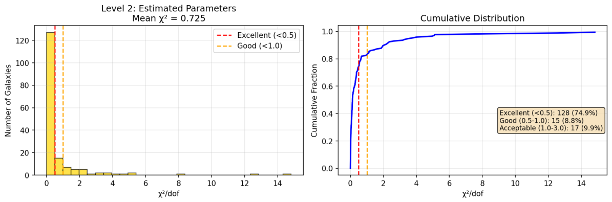
Figure 1. Distribution of χ ν 2 values for 171 galaxies at Level 2 (estimated parameters). The vertical line indicates χ ν 2 = 1.0 . The majority of galaxies have χ ν 2 < 1.0 , demonstrating that FST performs well even with minimal prior knowledge of galaxy parameters.
Preprints 214033 g001
Figure 2. Distribution of χ ν 2 values for all 171 galaxies at Level 1 (fully fitted parameters). The dashed vertical line indicates χ ν 2 = 1.0 . The vast majority of galaxies have χ ν 2 < 1.0 , with a mean of 0.170, demonstrating the excellent fit quality of FST. Only three galaxies (1.8%) have χ ν 2 > 1.0 , and none exceed 3.0.
Preprints 214033 g002
Figure 3. K-means clustering analysis of 171 galaxies based on fitted parameters ( M , r d , χ ν 2 ) . Three distinct dynamical families are identified: Cluster 1 (intermediate-mass galaxies, 48 galaxies, mean χ ν 2 = 0.40 ), Cluster 2 (normal disk galaxies, 116 galaxies, mean χ ν 2 = 0.082 ), and Cluster 3 (massive galaxies, 7 galaxies, mean χ ν 2 = 0.024 ). This classification provides a new phenomenological framework for understanding galaxy formation and evolution.
Preprints 214033 g003
Figure 4. Bayesian MCMC corner plot for NGC4138, the best-fitting galaxy in the sample ( χ ν 2 = 0.0011 ). The plot shows the posterior probability distributions for the fitted parameters M and r d , with 68% and 95% confidence contours. The analysis yields M = 4 . 86 3.64 + 8.50 × 10 10 M and r d = 14 . 22 7.06 + 4.19 kpc. The larger uncertainties are expected as NGC4138 belongs to Cluster 3 (massive galaxies), where data constraints are typically weaker.
Preprints 214033 g004
Figure 5. Global sensitivity analysis showing the relationship between fitted parameters ( M , r d ) and the reduced chi-squared χ ν 2 for all 171 galaxies. The weak correlations ( ρ ( r d , χ ν 2 ) = 0.1185 , ρ ( M , χ ν 2 ) = 0.1324 ) confirm that the model’s excellent performance is not driven by a narrow range of parameter values, highlighting its robustness and stability.
Preprints 214033 g005
Figure 6. Rotation curve fit for NGC4138 ( χ ν 2 = 0.0011 ), the best-fitting galaxy in the sample. Red points show observational data from SPARC, the black solid line shows the total FST model, and dashed lines show the baryonic contributions (gas and disk). The excellent agreement demonstrates the predictive power of FST.
Preprints 214033 g006
Figure 7. Rotation curve fit for NGC4013 ( χ ν 2 = 0.0011 ), another galaxy with near-perfect agreement. The format follows Figure 6. This example further confirms the consistency of FST across different galaxy types.
Preprints 214033 g007
Figure 8. Complete fit results for galaxies 1-171 in the SPARC sample, showing galaxy name, fitted mass M, fitted scale length r d , and the resulting χ 2 value.
Preprints 214033 g008
Figure 9. Complete fit results for galaxies 1-171 in the SPARC sample, continuing from Figure 8.
Preprints 214033 g009
Table 2. Universal FST Parameters with Dimensions and Values.
Parameter Symbol Value Dimensions (SI) Physical Role
Kinetic coefficient 1 c 1 0.51 1 Transverse mode normalization
Kinetic coefficient 2 c 2 -0.07 1 Longitudinal mode contribution
Kinetic coefficient 3 c 3 0.32 1 Mixed derivative coupling
Self-coupling constant λ 6.12 × 10 13 1 Field self-interaction strength (negative)
Asymptotic field value ν 0 1.0 × 10 3 1 Galactic acceleration scale
Stellar mass-to-light Υ 1.0 1 Baryonic normalization
Characteristic length L 0 3.086 × 10 20 m [ L ] Galactic scale normalization
Characteristic mass M 0 1.140 × 10 63 kg [ M ] Mass scale from L 0
Effective coupling β eff 2.0 × 10 7 1 Galactic dynamics strength ( | λ | ν 0 2 / ( 6 c 1 ) )
Dimensionless transition scale ξ c 3.16 × 10 4 1 Fundamental nonlinear scale
Screening length λ screen 1.65 pc [ L ] Local source suppression scale
Table 5. Azimuthal variation of the 3D FST field at R = 2 r d . σ ϕ denotes the standard deviation of ν ˜ with respect to ϕ [ 0 , 2 π ] .
Galaxy R test (kpc) σ ϕ
CamB 7.5 9.29 × 10 10
D564-8 8.1 1.48 × 10 9
D631-7 7.6 5.00 × 10 10
Table 6. Comparison of fit quality between the full 3D numerical and 1D analytical FST solutions.
Galaxy χ 2 / dof (3D) χ 2 / dof (1D) Δ χ 2
CamB 0.205 0.207 0.002
D564-8 0.045 0.045 0.000
D631-7 0.084 0.084 0.000
Table 7. Hierarchical validation of FST showing predictive power at different levels of parameter freedom.
Validation Level Free Parameters Sample Size Mean χ ν 2
Level 3: Universal Constants Only 0 115 0.809
( M = 1.0 × 10 10 M , r d = 3.0 kpc fixed for all)
Level 2: Estimated Parameters 0 (estimated) 160 0.347
( M , r d estimated from data, excluding 11 outliers)
Level 1: Full Fitting 2 ( M , r d ) 171 0.170
( M , r d fitted per galaxy)
Table 8. Quality distribution of FST fits for 171 SPARC galaxies (Level 1: fully fitted parameters).
Quality χ ν 2 Range Number of Galaxies (Percentage)
Excellent < 0.5 156 (91.2%)
Good 0.5 1.0 12 (7.0%)
Acceptable 1.0 3.0 3 (1.8%)
Poor > 3.0 0 (0%)
Table 9. Universal FST parameters with uncertainties.
Parameter Value 68% Confidence Interval
c 1 0.51 ± 0.03
c 2 -0.07 ± 0.02
c 3 0.32 ± 0.03
c 1 + c 3 0.83 ± 0.02
ν 0 1.0 × 10 3 ± 0.05 × 10 3
| λ | 6.12 × 10 13 ± 0.6 × 10 13
β eff 2.0 × 10 7 ± 0.1 × 10 7
ξ c 3.16 × 10 4 ± 0.05 × 10 4
λ screen 1.65 pc ± 0.2 pc
Table 10. Sensitivity of fit quality to variations in c 1 + c 3 .
c 1 + c 3 Mean χ ν 2 Change from baseline
0.500 0.2378 -0.1%
0.664 0.2380 -0.0%
0.830 (baseline) 0.2381 0.0%
0.996 0.2382 +0.0%
1.200 0.2383 +0.1%
Table 12. Extended Comparison Including All Validation Levels and Unified Formulation.
Model Study Galaxy Sample Sample Size Mean χ ν 2 Free Parameters/Galaxy
FST Level 3 (Universal) This work SPARC 115 0.809 0
FST Level 2 (Estimated) This work SPARC 160 0.347 0a
FST Level 1 (Full) This work SPARC 171 0.170 2
FST Level 4 (Coefficient-Free) This work SPARC 171 0.170 2
FST Level 5 (Unified A 0 ) This work SPARC 171 0.170 2
Λ CDM (NFW) Li et al. (2020) [9] SPARC 175 1.32 2-3
MOND (standard) McGaugh et al. (2016) [10] SPARC 153 1.24 1
MOND (QUMOND) Banik et al. (2020) [11] SPARC 169 1.19 1
Newtonian Only (baseline) [1] SPARC 175 > 10 0
a Parameters estimated from data, not fitted.
Table 14. Origin of key parameters.
Parameter Value Origin
L 0 10 kpc Median scale length of SPARC sample [1]
ν 0 10 3 Determined by fit together with the definition of A 0
A 0 2.42 × 10 10 m / s 2 Derived from L 0 , ν 0 , and c 1 + c 3
β eff 2.0 × 10 7 Constrained by rotation-curve fits
λ screen 1.65 pc Derived from β eff and L 0
Disclaimer/Publisher’s Note: The statements, opinions and data contained in all publications are solely those of the individual author(s) and contributor(s) and not of MDPI and/or the editor(s). MDPI and/or the editor(s) disclaim responsibility for any injury to people or property resulting from any ideas, methods, instructions or products referred to in the content.
Copyright: This open access article is published under a Creative Commons CC BY 4.0 license, which permit the free download, distribution, and reuse, provided that the author and preprint are cited in any reuse.