Submitted:
06 February 2026
Posted:
06 February 2026
You are already at the latest version
Abstract
Repeated measures ANOVA is the statistical method for comparing means of the same sample measured at least two different times, or two different contexts. It may also be used to compare means between two or more related groups. This paper serves as a tutorial for repeated measures ANOVA using R. It will introduce readers to parametric, nonparametric and robust one-way repeated measures ANOVA using the rstatix, afex, WRS2, and ARTool packages.
Keywords:
repeated measures ANOVA
; analysis of variance
; statistics education
; statistical programming
; R programming
; repeated measures analysis of variance
Introduction
Repeated Measures ANOVA
Repeated measures ANOVA (RMA), also called dependent ANOVA, is a method for comparing two or more means of related groups, or (more commonly) the same group measured at two or more times, contexts, or conditions. Like independent ANOVA it may be used for two or more means, and also uses the assumption of normality of outcomes at each level if the independent variable. Sphericity is defined as the equality of variances of the differences between each pair of treatment levels, and is also an assumption for the use of parametric RMA (Field, 2013). The assumption of sphericity therefore requires at least three levels of the independent variable. Sphericity is assessed by Mauchly’s test of sphericity, and this is standard output for software computing RMA. If it is non-significant, sphericity may be assumed. If significant, corrections exist. These include the Greenhouse-Geisser and Huynh-Feldt corrections (Field, 2013). For violations of normality, several methods exist such as Friedman’s ANOVA. Whereas the assumption of independent observations exists for independent ANOVA, RMA assumes related observations (i.e., relatedness). Hence, this method is typically used in studies where participants are measured at two or more timepoints, contexts, or conditions. It may also be potentially used to study related samples (e.g., comparing the same traits of several generations of plants or bacteria). Repeated measures ANOVA also requires complete data for all timepoints. Any case with incomplete data will be excluded from analysis, and standard repeated measures ANOVA may not be used. For studies requiring repeated measurements, where the violations of related observations and complete data occur, methods such as multilevel models may be used. Finally, for analyses with more than two levels, post hoc comparisons may be used. A brief discussion of post hoc comparisons and their descriptions is listed below.

Table 1.
List of ANOVA pairwise comparisons/post hoc tests.
| Pairwise comparison | Description of method |
| Bonferroni | Single step. Strong control of Type I error/family-wise error rate (FWER). However, strong control may lead to Type II error. |
| Dunnett | Single step. Designed to compare treatment groups to a control group. |
| Benjamini-Hochberg/False Discovery Rate (BH/FDR) | Controls false discovery rate (FDR) rather than FWER; more powerful than Bonferroni, Holm. |
| Benjamini-Yekutieli (BY) | Same as above. |
| Hochberg | Step-up. Similar to Tukey, but better for unbalanced designs. More powerful than Bonferroni. |
| Holm | More powerful, step-down modification of Bonferroni procedure, while controlling FWER. |
| Hommel | Step up. Generally more powerful than Holm. |
| Sidak | Single step, though a step down version also exists. Stringent Type I error control, but more powerful than Bonferroni. |
| Scheffe | Single step. Flexible, with lower power compared to Tukey for pairwise comparisons. |
| Tukey HSD (Honestly Significant Difference) | Single step. Widely used method across several fields; use for balanced designs. |
| Games-Howell | Single step. Use when the assumption for equal variances is violated. |
| Dunn | Single step. Non-parametric test; use with non-parametric ANOVA. |
| Fisher’s Least Significant Differences | Single step. Does not control for inflation of Type I error; generally not recommended for post hoc testing. |
The R environment
R is a free and open-source environment for statistical computing, supported by a worldwide network of scientists and programmers. It contains add-on packages for statistics, data science, and related areas such as geographical information systems. These qualities make R a powerful tool for teaching and data analysis. However, R requires coding which may intimidate new users, and may compound statistical anxiety in introductory statistics courses using R. R may be used with an integrated development environment such as RStudio (Posit, 2025) to more easily manage data, packages, and objects.
Repeated Measures ANOVA in R
There are several packages that implement RMA in R. The rstatix package (Kassambara, 2025) is a comprehensive option for both parametric and nonparametric RMA. Other packages include afex (Singmann, et al., 2025) combined with datawizard (Patil, et al, 2022), and emmeans (Lenth & Piakowski, 2025) for parametric RMA. The ARTool package (Wobbrock at al., 2011) combined with emmeans are also a good option for nonparametric analysis. The WRS2 package also offers a robust option as well as robust post hoc tests. The tidyr package (Wickham et al., 2024) is used to demonstrate reformatting of data from long to wide, and vice versa. The ggstatsplot package (Patil, 2021) will be used for visualization.
For Type I sums of squares in ANOVA analysis, the order in which predictors are entered matters. This method is not recommended for repeated measures designs, as they do not evaluate main effects or interactions. The base R package uses this variant only (Field, Miles & Field, 2012). Conversely, Type II sums of squares takes all main effects into consideration, while ignoring higher order (interaction) effects. Type III sums of squares evaluates the effects (main and interaction), taking all other effects into context, and is also used for unbalanced designs. It is the default used by commercial packages that implement RMA like SPSS, and for R packages such as rstatix (Field, Miles & Field, 2012; Kassambara, 2025). The second problem with using the base R functions is that they do not produce tests of sphericity. Hence repeated measures ANOVA using the base R package will be omitted from this tutorial.
The packages presented here use the long data format. This means that the time or context variable has one dedicated column with all of its levels, and each observation’s timepoint is in a separate row. Hence, for a study that measures four timepoints, each participant will have four rows of data. An ID number is used so that the software can discern every participant across all levels. This is in contrast to the wide format, where every level of time or condition has its own dedicated column, and therefore each participant has a dedicated row across several columns. This latter format is used for packages such as SPSS (Armonk, NY), and JASP (JASP Team, 2025). Syntaxes for conversion from wide long format and vice versa will be shown.
Objects
An object is a way of summarizing, storing, and managing some entity created, or found in R. For example, an object may be used for a dataset. For example, data1<-c(2, 4, 6, 17) assigns the object “data1” to four scores. In the table below, a dataset is converted from long to wide format, and a new object is assigned to the newly formatted data. Users are encouraged to create and manage objects at their discretion.
Data
The premise for this dataset is that a group of students engaged in a four-phase learning program designed to improve their performance in an undergraduate applied statistics course. Student performance was measured at each phase to evaluate the program’s effectiveness.
Method
Once the datasets have been uploaded into RStudio, the following steps may be taken to reformat data if needed, and for analysis. For parametric analysis, rstatix as well as afex and emmeans will be used. The rstatix package, WRS2, as well as ARTool and emmeans will be used. The syntaxes for converting from long to wide and vice versa using the tidyr package are shown below.
Table 2.
Syntaxes for conversion of formats.
| Syntax | Purpose |
| library(tidyr) | Loads the package |
| pivot_wider(rma, names_from = phase, values_from = score) | Converts data from long format to wide format. |
| rma_wide<-pivot_wider(rma, names_from = phase, values_from = score) | Assigns a new object to the newly created data. |
| View(rma_wide) | Checks to make sure dataset was properly converted. |
| rma_long<-pivot_longer(rma_wide, cols = -ID, names_to = "phase", values_to = "score") | Converts data from wide to long format. |
Parametric Repeated Measures ANOVA
Repeated Measures ANOVA Using the Rstatix Package
The following syntaxes are used to compute RMA. Both the rstatix and afex packages require the long format for analysis. The ggstatsplot package is used to create a custom plot to visualize the analysis.
Table 3.
Parametric Repeated Measures ANOVA syntax using rstatix.
| Package | Syntax | Purpose |
| library(rstatix) library(afex) library(emmeans) |
||
| rstatix | rma_desc<-rma %>% group_by(phase) %>% get_summary_stats(score) |
Creates object for descriptive statistics table. |
| rma_desc | Shows descriptive statistics. | |
| rm_rstatix<-anova_test(data = rma, dv = score, wid = ID, within = phase) | Repeated measures ANOVA in rstatix. General eta squared is the default effect size. | |
| rm_rstatix0<-anova_test(data = rma, dv = score, wid = ID, within = phase, effect.size = "pes") | Similar to the above. Although the general interpretation is similar, note the difference between general and partial eta squared. | |
| rm_rstatix_post_hoc<- rma%>% pairwise_t_test(score~phase, paired = TRUE, p.adjust.method = "holm") | Post hoc tests using holm adjustment. Other options include Bonferroni, Hochberg, Hommel, and others. |
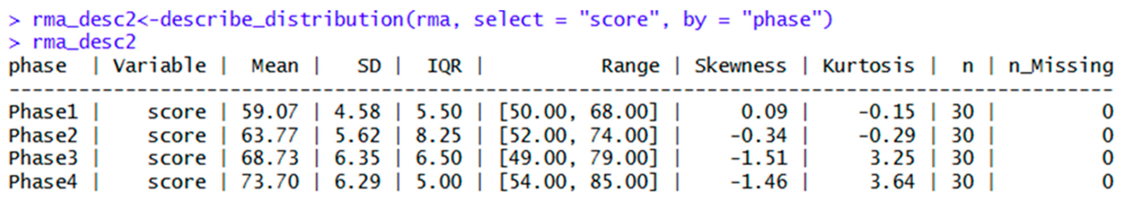
Figure 1.
Descriptive statistics.
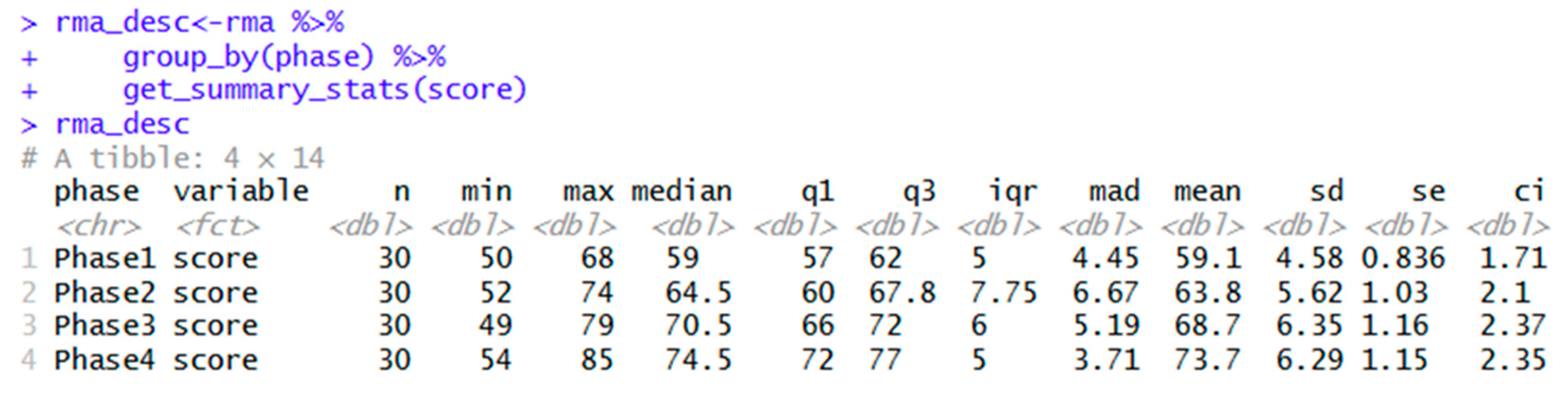
The default effect size for rstatix is general eta squared as shown below. Note the difference from partial eta squared, which tends to be more upward biased (Ellis, 2017).
Figure 2.
RM ANOVA summary table.
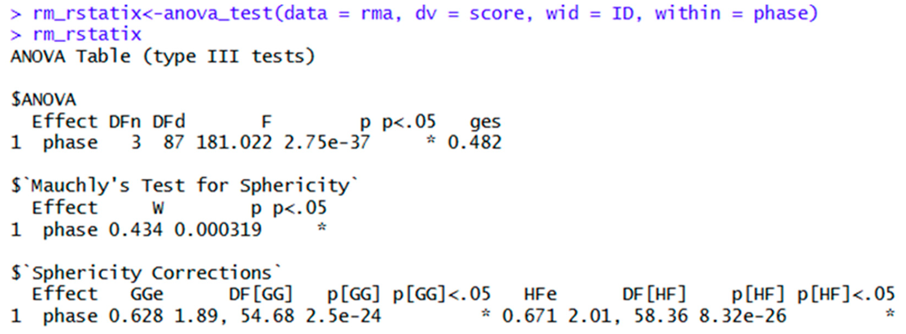
If the assumption of Sphericity were met, the ANOVA table could be used, and reported as follows: F(3, 87) = 181, p < .01, η2g = .48. However, Mauchly’s Test of Sphericity is violated. Hence, either the Greenhouse-Geisser or Huynh-Feldt adjustment should be reported. The Greenhouse-Geisser adjustment is reported as follows: F(1.89. 54.68) = 181, p < .01, η2g = .48. In other words, the F value from the second line of the output is reported, along with the Greenhouse-Geisser adjusted degrees of freedom and the p-value from the “Sphericity Corrections” section. Alternatively, the Huynh-Feldt adjustment can be reported as follows: F(2.01, 58.36) = 181, p < .01, η2g = .48. Feel free to round as appropriate, e.g. F(2, 58.4) = 181, p < .01, η2g = .48.
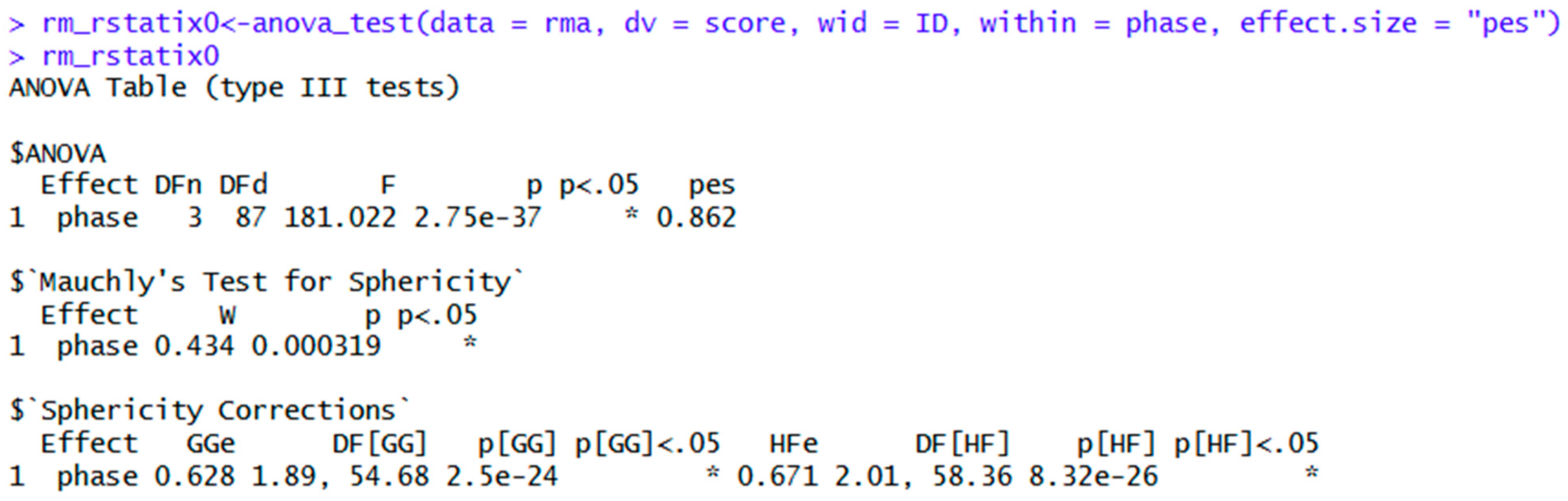
If partial eta squared is chosen as the effect size, then report as follows: F(1.9. 54.7) = 181, p < .01, η2p = .86. Note that the latter report uses the Greenhouse-Geisser adjustment, and the Huynh-Feldt adjustment may be reported instead.
Figure 3.
ANOVA table with partial eta squared effect size.
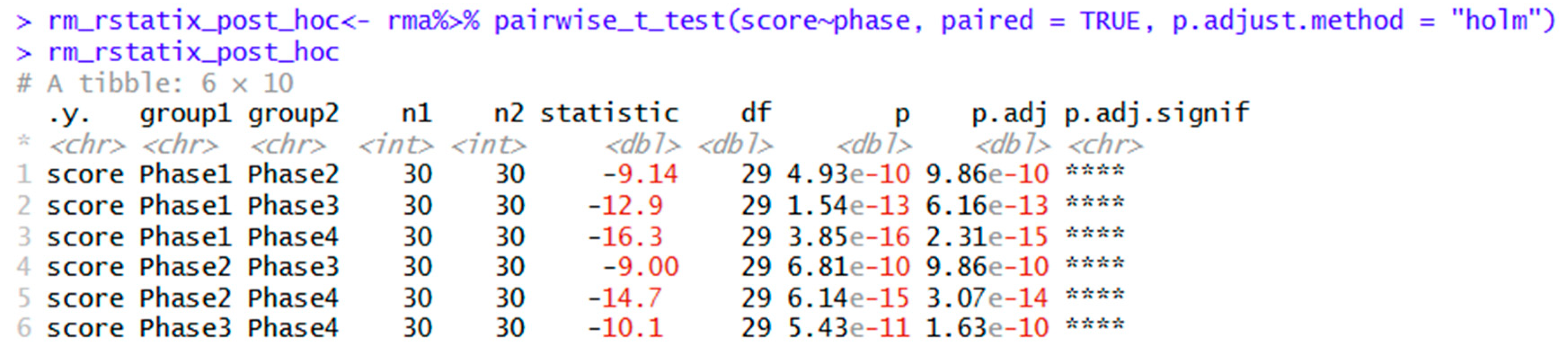
Finally, the output for the Holm post hoc test is shown below. Pairwise comparisons show that all means differed from one another. The descriptive statistics table shows that the score increased significantly from Phase 1 through Phase 4.
Figure 4.
Post hoc tests using Holm adjustment for multiple comparisons.
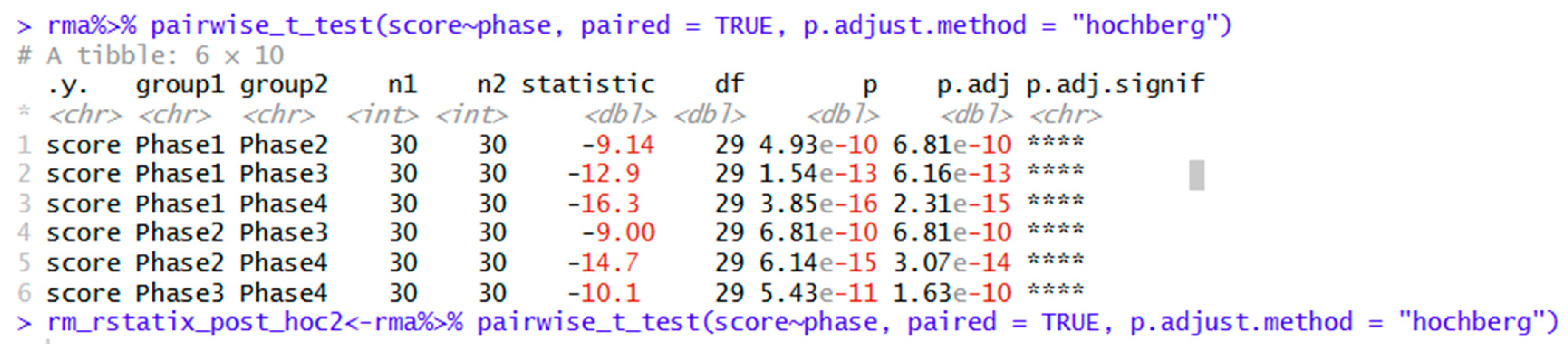
Other options for post hoc testing are shown in Table 2. Simply use the adjustment you wish in the “p.adjust.method” command in all lower-case letters. For example, the Hochberg method is shown below.
Figure 5.
Post hoc tests using Hochberg adjustment for multiple comparisons.
Repeated Measures ANOVA Using Afex and Emmeans
The afex package may also be used to compute RMA in tandem with the emmeans package to compute post hoc analysis. Visualization using the ggstatsplot package is also shown in this section.
Table 4.
Parametric Repeated Measures ANOVA syntax using datawizard, afex and emmeans.
| Package | Syntax | Purpose |
| library(afex) library(datawizard) library(emmeans) library(ggstatsplot) |
||
| datawizard | describe_distribution(rma, select = "score", by = "phase") | Descriptive statistics |
| afex | rm_afex<-aov_ez(data = rma, id = "ID", dv = "score", within = "phase", anova_table = list(es = "pes")) | Repeated measures ANOVA in afex. |
| rm_afex | Shows ANOVA table with any adjustments. Greenhouse-Geisser is the default method. | |
| summary(rm_afex) | Same as above, but with more detail. | |
| rm_afex_HF<- aov_ez(data = rma, id = "ID", dv = "score", within = "phase", anova_table = list(es = "pes", correction = "HF")) | Use this syntax to get Huynh-Feldt adjustment instead. | |
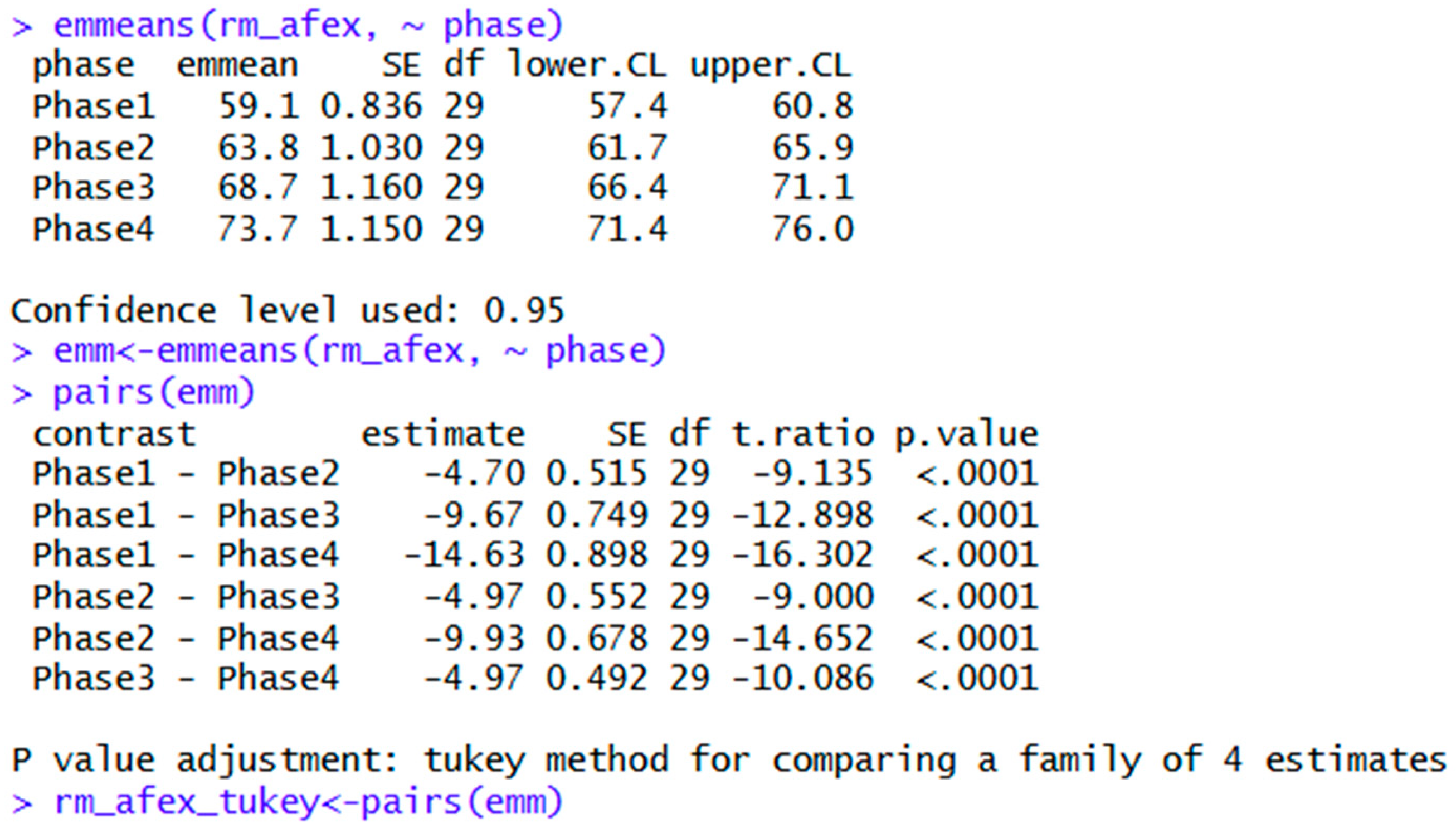
| emmeans | emm<-emmeans(rm_afex, ~ phase) | Shows means and other parameters for each level of the ANOVA. |
| pairs(emm) | Pairwise comparisons; Tukey post hoc is the default. | |
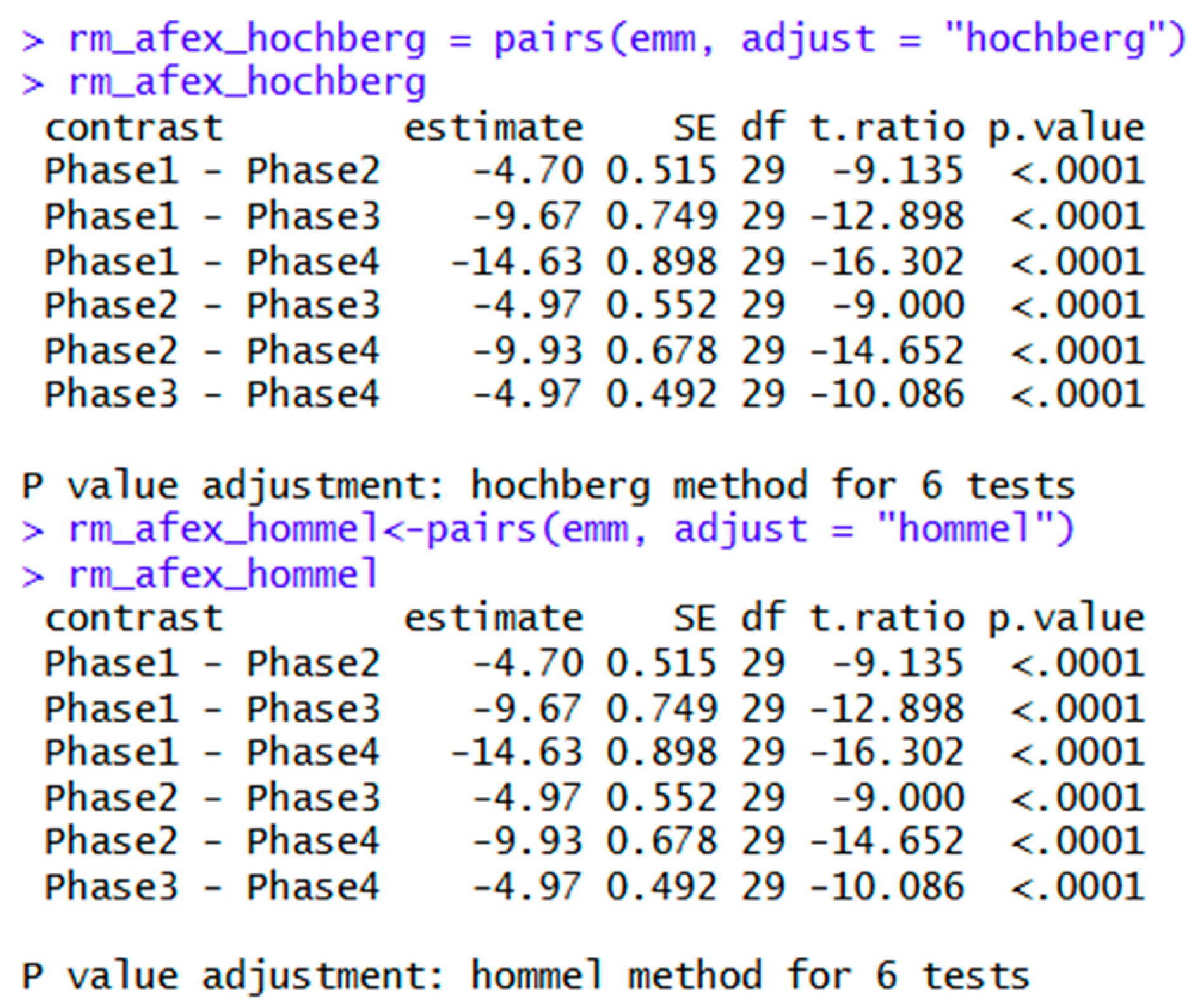
| rm_afex_hochberg = pairs(emm, adjust = "hochberg") | Creates an object for Hochberg post hoc tests. Bonferroni, Hommel, Holm, Scheffe, Sidak, and other options may be found here. | |
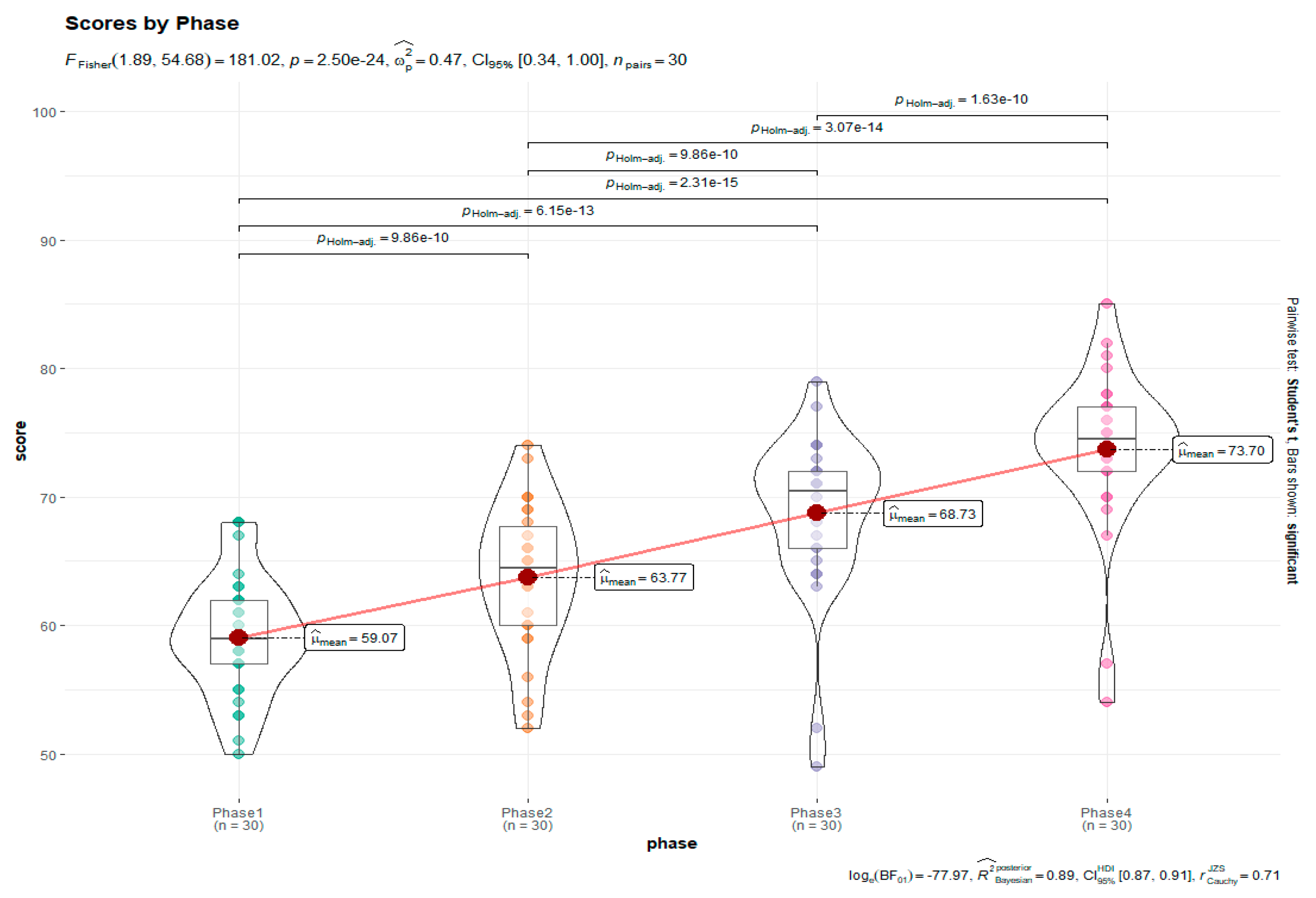
| ggstatsplot | rmplot<-ggwithinstats(data = rma, x = phase, y = score, type = "parametric", pairwise.comparisons = TRUE, p.adjust.method = "holm", title = "Scores by Phase") |
Visualization. |
The afex package is also capable of computing parametric RMA analyses. Unlike rstatix, it does not offer descriptive statistics or post hoc tests. These may be respectively obtained using the datawizard and emmeans packages. Descriptive statistics using the datawizard package is shown below.
Figure 6.
Descriptive statistics using the datawizard package.
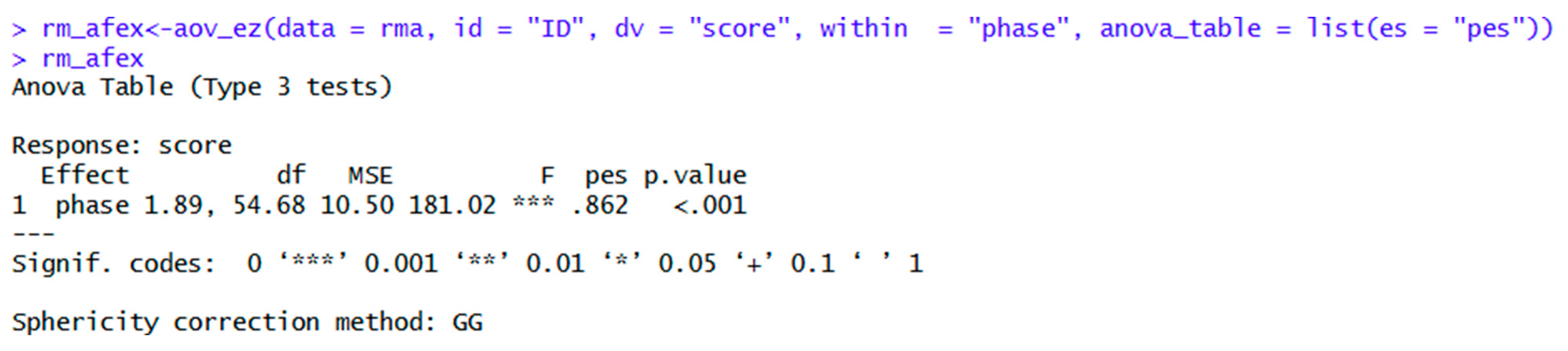
Note that the “aov_ez” command provides an abridged ANOVA table, while the summary command offers more detailed output. However, the abridged output mentions that the Greenhouse-Geisser adjustment is used, and also gives the adjusted degrees of freedom for this method. Therefore, this command intuitively suggests that Mauchly’s Test of Sphericity is violated.
Figure 7.
Repeated measures ANOVA table using afex.
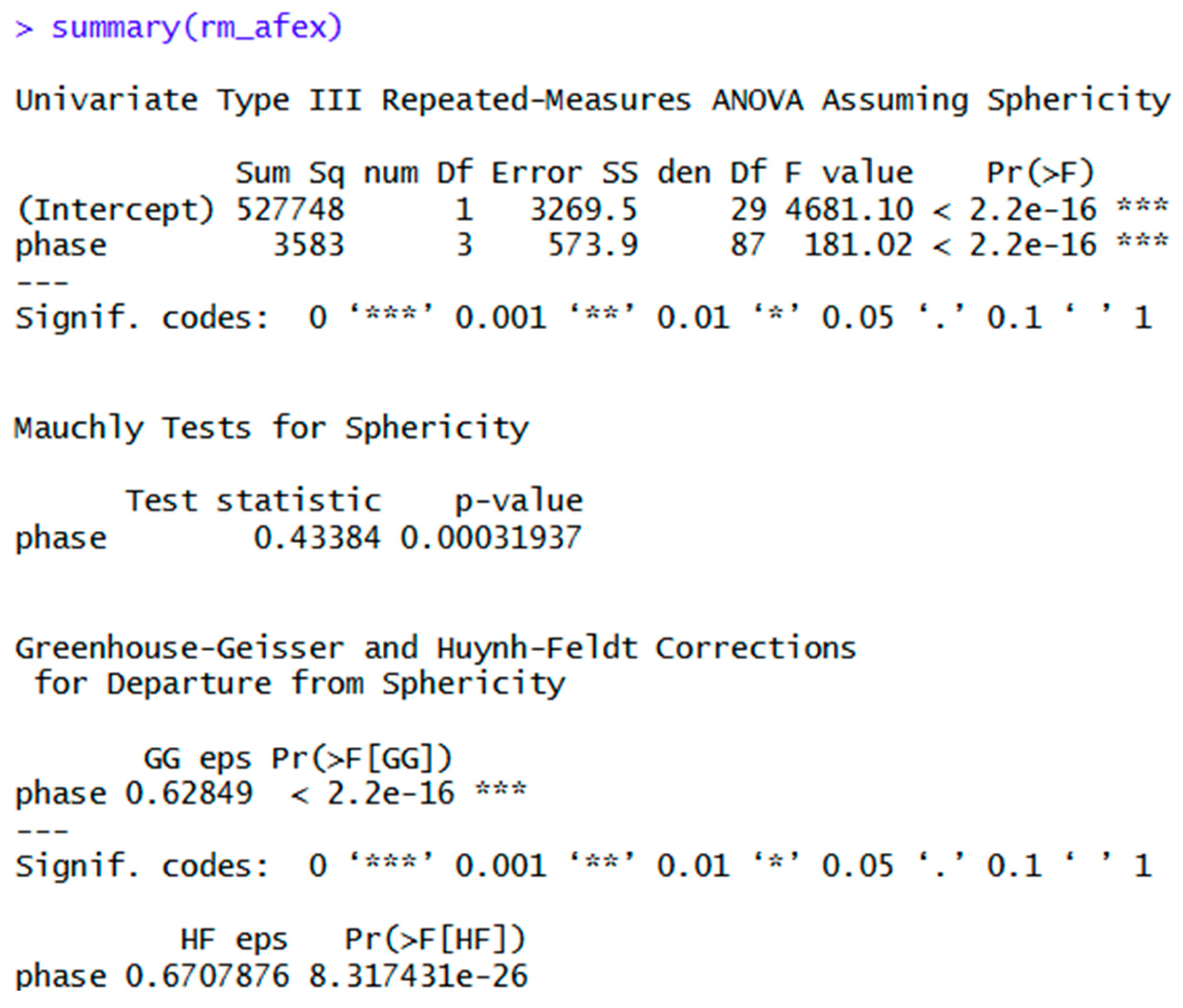
The more detailed output below does provide an actual value for Mauchly’s Test, and p-values for both adjustments, but does not offer the adjusted degrees of freedom for either.
Figure 8.
Detailed afex ANOVA output.
Post hoc testing may be obtained using the syntaxes below using the emmeans package. The Tukey adjustment is the default method.
Figure 9.
Tukey post hoc comparisons using emmeans.
Other post hoc tests may be obtained by specifying the adjustments as shown below.
Figure 10.
Hochberg and Hommel post hoc comparisons using emmeans.
Finally, visualization using the ggstatsplot package is shown below.
Figure 11.
Visualization using ggstatsplot.
Options for Violated Normality Assumptions
Friedman’s ANOVA Using Afex
Friedman’s ANOVA is a popular non-parametric option for heavily skewed data, or small sample sizes. The rstatix package also performs Friedman’s ANOVA. The syntaxes are shown below, with ggstatsplot used for visualization.
Table 5.
Friedman’s ANOVA using rstatix.
| Package | Syntax | Purpose |
| rstatix | friedman_rstatix<-friedman_test(data = rma, score~phase|ID) | Friedman’s ANOVA in rstatix. |
| fes<-friedman_effsize(data = rma, score~phase|ID) | Generates Kendall’s W. | |
| friedman_post_rstatix<-pairwise_wilcox_test(rma, score~phase, paired = TRUE, p.adjust.method = "holm") | Pairwise Wilcoxon tests with Holm adjustments. | |
| pairwise_wilcox_test(rma, score~phase, paired = TRUE, p.adjust.method = "bonferroni") | Same as above, except with Bonferroni adjustment. | |
| ggstatsplot | friedmanplot<-ggwithinstats(data = rma, x = phase, y = score, type = "nonparametric", pairwise.comparisons = TRUE, p.adjust.method = "holm", title = "Scores by Phase") | Visualization. This package is helpful as it also gives an APA style report and post hoc comparisons. |
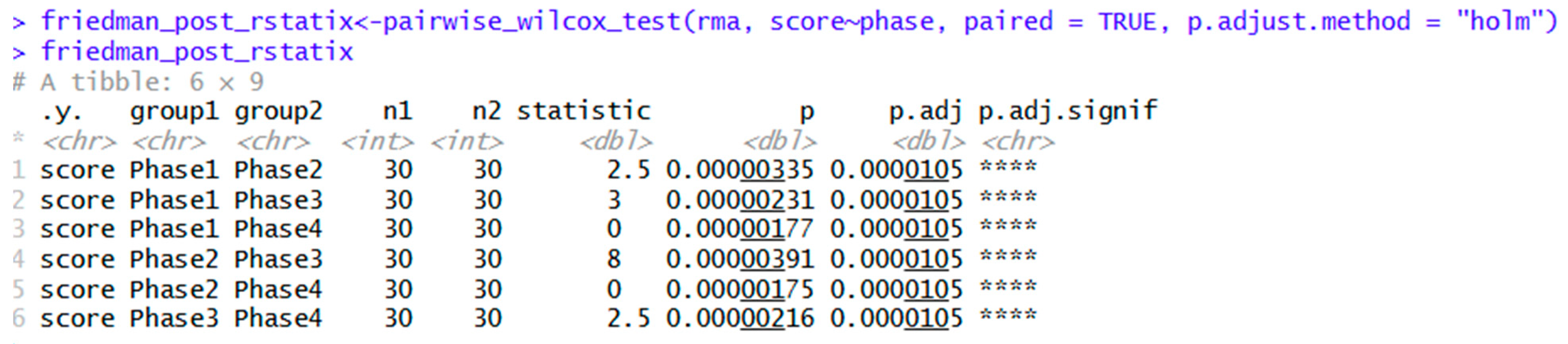
The Friedman test and Kendall’s W effect size outputs are shown below. They may be reported as follows: χ2Friedman(3, n = 30) = 80.5, p < .001, W = .90
Figure 12.
Friedman’s ANOVA output using rstatix.
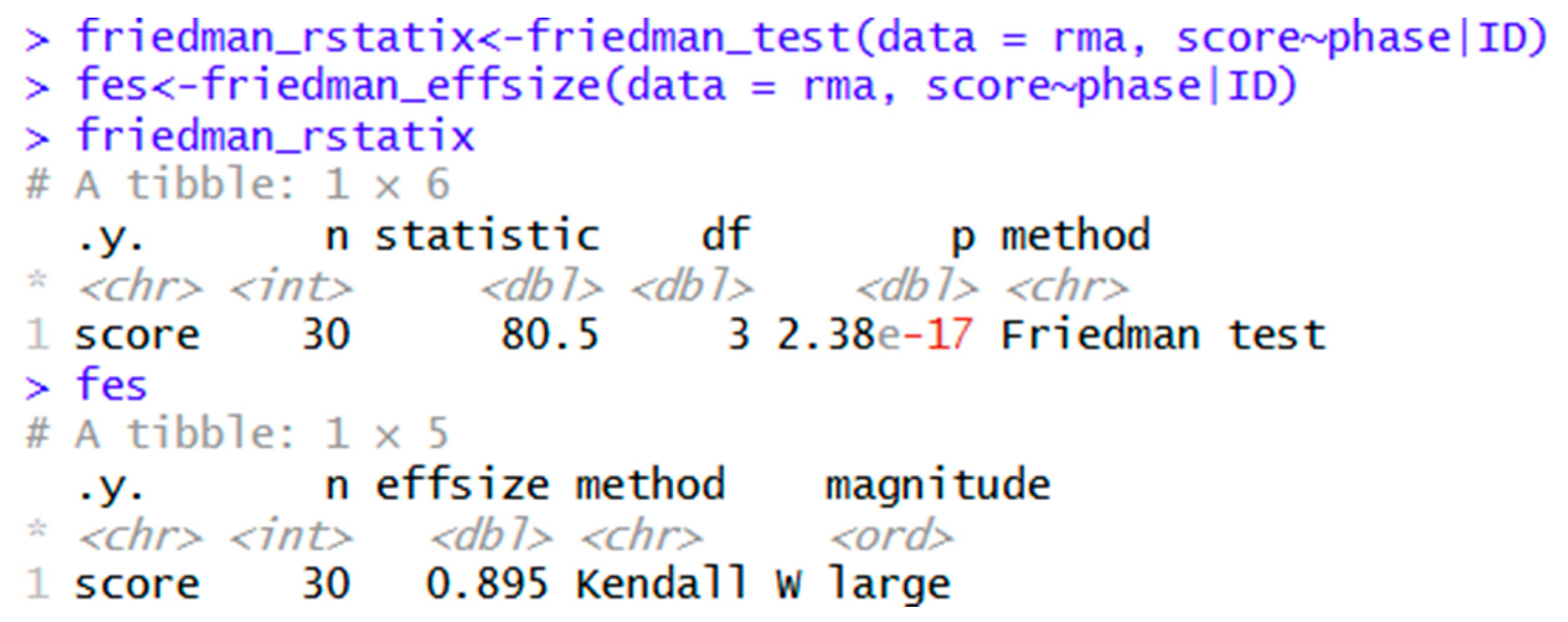
Figure 13.
Pairwise Wilcoxon post hoc comparisons with Holm adjustments.
Robust Repeated Measures ANOVA Syntax Using WRS2
The WRS2 package is another alternative. It offers robust and bootstrapped options for RMA and post hoc tests in case of violated assumptions. The syntaxes are shown in the table below.
Table 6.
Syntax for repeated measures ANOVA using WRS2.
| Package | Syntax | Purpose |
| library(WRS2) | ||
| WRS2 | robust_RM_WRS2<-rmanova(y = rma$score, groups = rma$phase, blocks = rma$ID) | Robust repeated measures ANOVA |
| with(rma, (rmanova(y = score, groups = phase, blocks = ID))) | Alternate syntax for above. | |
| rmmcp(y = rma$score, groups = rma$phase, blocks = rma$ID) | Post hoc tests for trimmed means. | |
| rmanovab(y = rma$score, groups = rma$phase, blocks = rma$ID) | Bootstrapped robust ANOVA. | |
| rmanovab(y = rma$score, groups = rma$phase, blocks = rmaf$ID, nboot = 2000) | Same as above, specifying 2000 bootstrapped samples. | |
| pairdepb(y= rma$score, groups = rma$phase, blocks = rma$ID, nboot = 2000) | Bootstrapped post hoc tests for the above ANOVA. |
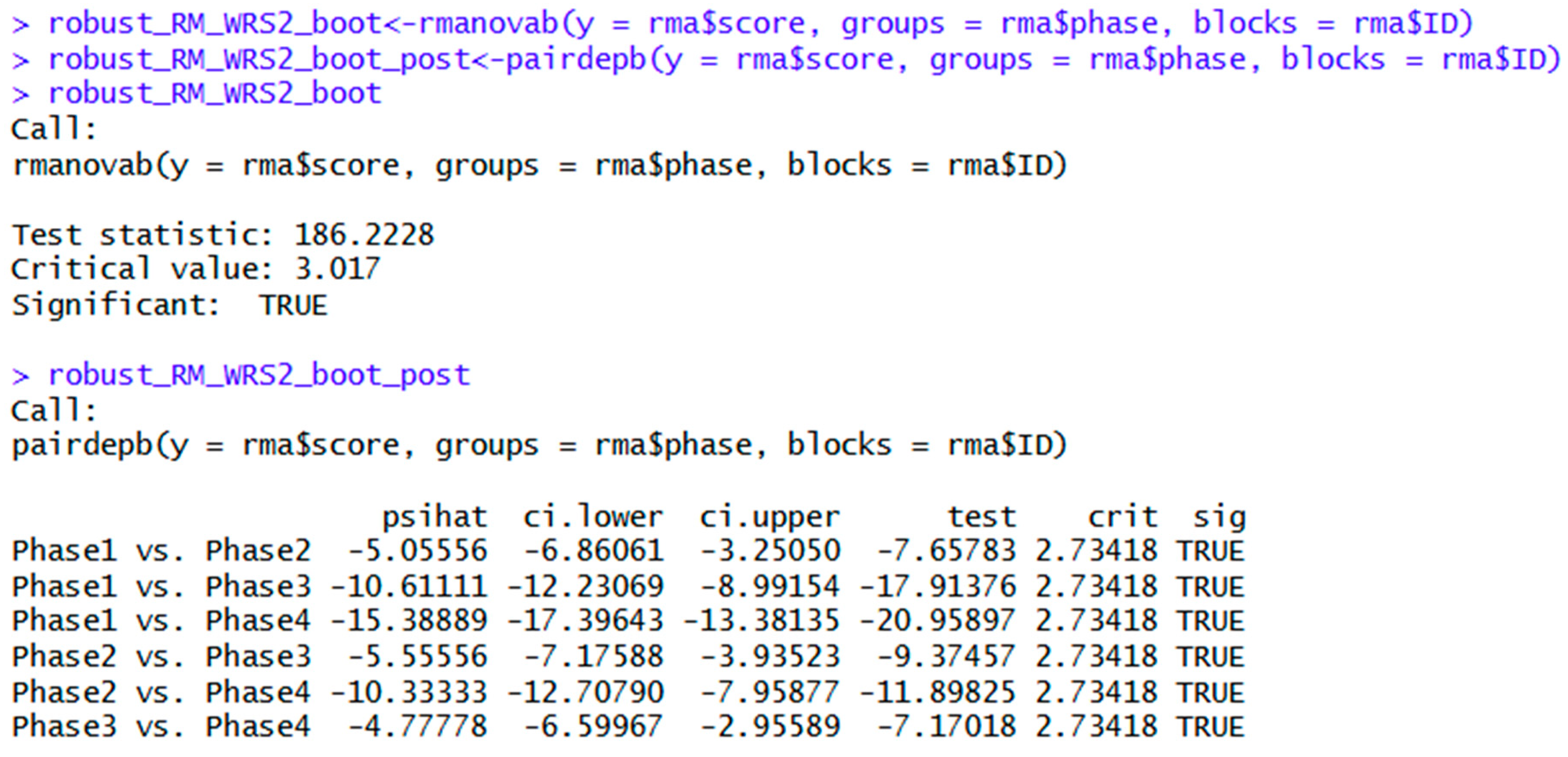
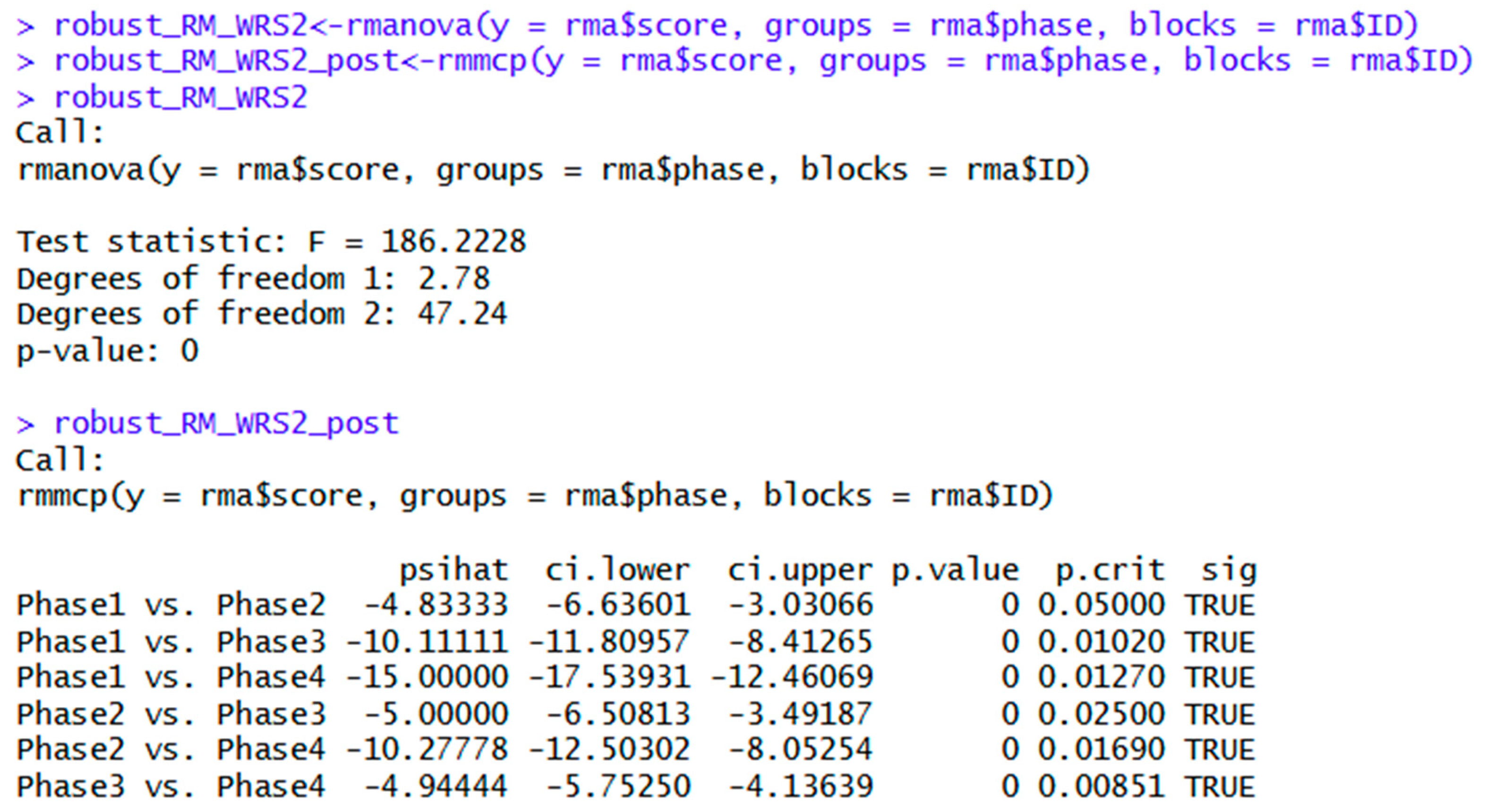
The first option for WRS2 is repeated measures ANOVA with 20% trimmed means. The null hypothesis is rejected, and should be reported as follows: F(2.78, 47.24) = 186.2, p < .001. The interpretation is exactly the same as the Friedman’s ANOVA in rstatix. However, a disadvantage of the WRS2 package is that it does not offer an effect size for RMA.
Figure 14: Robust one-way repeated measures ANOVA using WRS2
The WRS2 package also allows bootstrapped robust ANOVA and post hoc tests, as shown below. The overall null hypothesis is also rejected using this method. The bootstrapped robust RMA showed a significant effect of phase on score, as the test statistic (186.2) exceeded the critical value of 3.0, thus rejecting the null hypothesis. Note the interpretation of the post hoc tests is also similar to the rstatix analysis.
Figure 15.
Bootstrapped robust one-way repeated measures ANOVA using WRS2.
Aligned Rank Transformed ANOVA Using ARTool
The ARTool package is another option for nonparametric analysis. While specialized for factorial designs (Wobbrock et al., 2011), its use for one-way RMA is demonstrated below. It is somewhat more labor intensive than WRS2, and may be suitable for more advanced R users. It may be used with the effectsize and emmeans packages to obtain effect sizes and post hoc tests respectively. The syntaxes and workflow are shown in the table below.
Table 7.
Syntaxes for ANOVA of aligned rank transformed data using ARTool, effectsize, and emmeans packages.
Table 7.
Syntaxes for ANOVA of aligned rank transformed data using ARTool, effectsize, and emmeans packages.
| Package | Syntax | Purpose |
| library(ARTool) | ||
| rma$ID <-factor(rma$ID) | Convert the ID variable into a factor. | |
| rma$phase <-factor(rma$phase) | Same for independent variable. | |
| ARTool | artmodel<-art(score ~ phase + Error(ID), data = rma) | Transformation of repeated measures data using ARTool. |
| artanova<- anova(artmodel) | Repeated measures ANOVA of aligned rank transformed data in ARTool. | |
| artanova | Shows ANOVA table. | |
| art_phase<-artlm(artmodel, "phase") | ||
| effectsize | eta_squared(art_phase) | Partial eta squared. |
| art_effectsize2<-eta_squared(art_phase, partial = FALSE) | Generalized eta squared. | |
| eta_squared(art_phase, partial = FALSE, generalized = TRUE) | Same as above. | |
| emmeans | art_post <-emmeans(art_phase, pairwise ~ phase) | Pairwise comparisons with Tukey adjustment as the default method. Multiple post hoc tests are shown for demonstration only. Choose one post hoc test ahead of time. |
| emmeans(art_phase, pairwise ~ phase, adjust = "bonferroni") | Bonferroni adjustment. | |
| art_post_holm<-emmeans(art_phase, pairwise ~ phase, adjust = "holm") | Holm adjustment. Also offers Scheffe, Sidak, and others. |
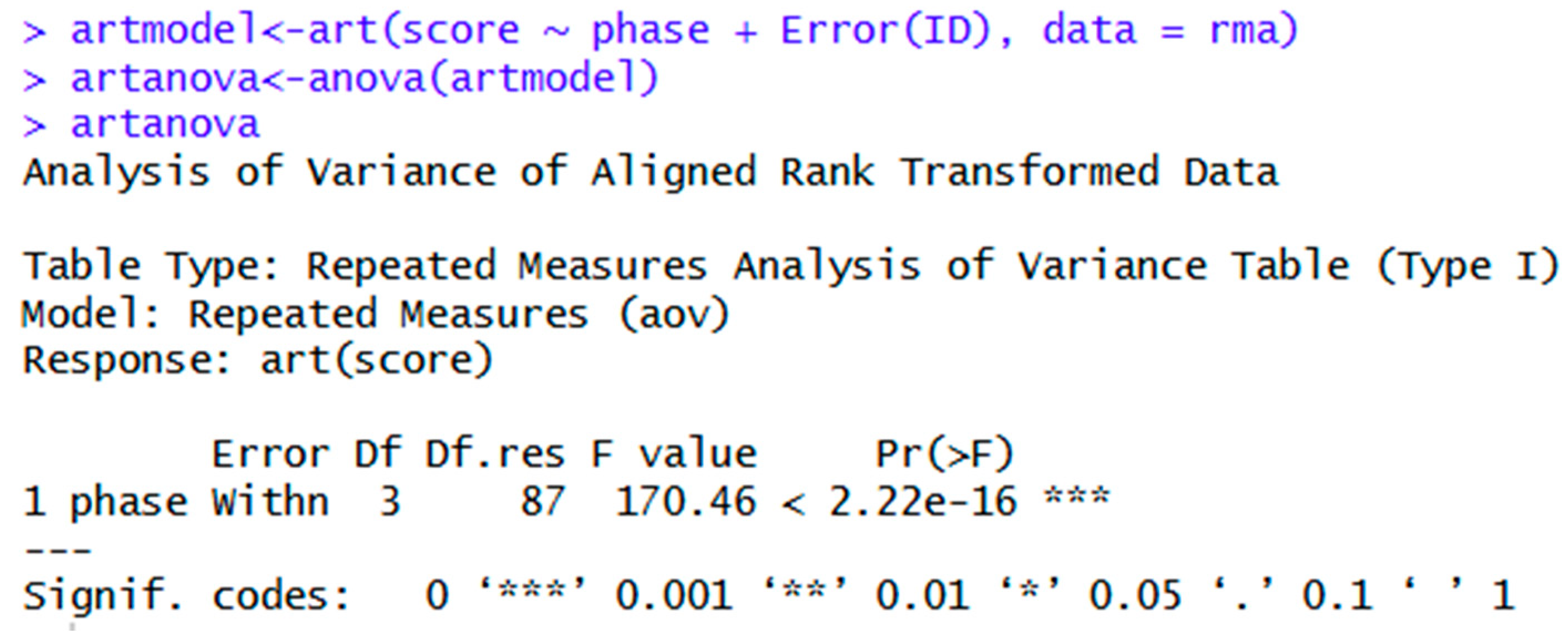
The figure below shows the ANOVA table. Note that obtaining the ANOVA table is comprised of two steps: transforming the data, followed by the ANOVA analysis.
Figure 16.
Syntax and output for ANOVA of aligned rank transformed data.
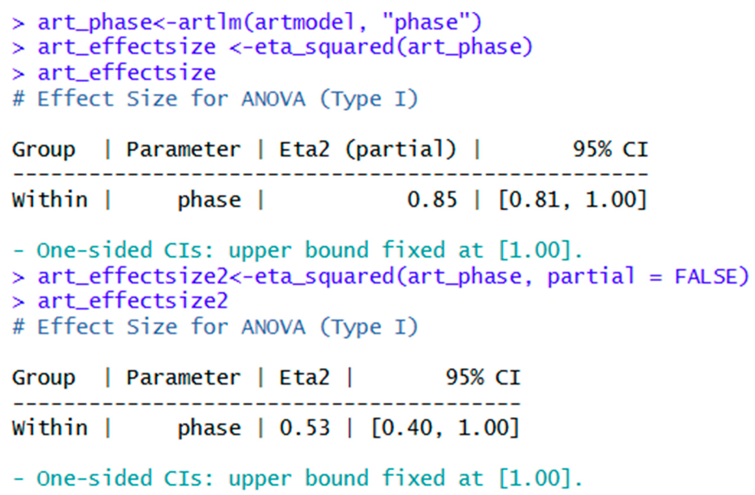
The effectsize package may be used to obtain either partial eta squared or generalized eta squared. Note that partial eta squared tends to be upwardly biased. The analysis may be reported as follows: F(3, 87) = 170.5, p < .001, η2g = .53 for generalized eta squared, or F(3, 87) = 170.5, p < .001, η2p = .85 for partial eta squared.
Figure 17.
Effect sizes for ANOVA of aligned rank transformed data.
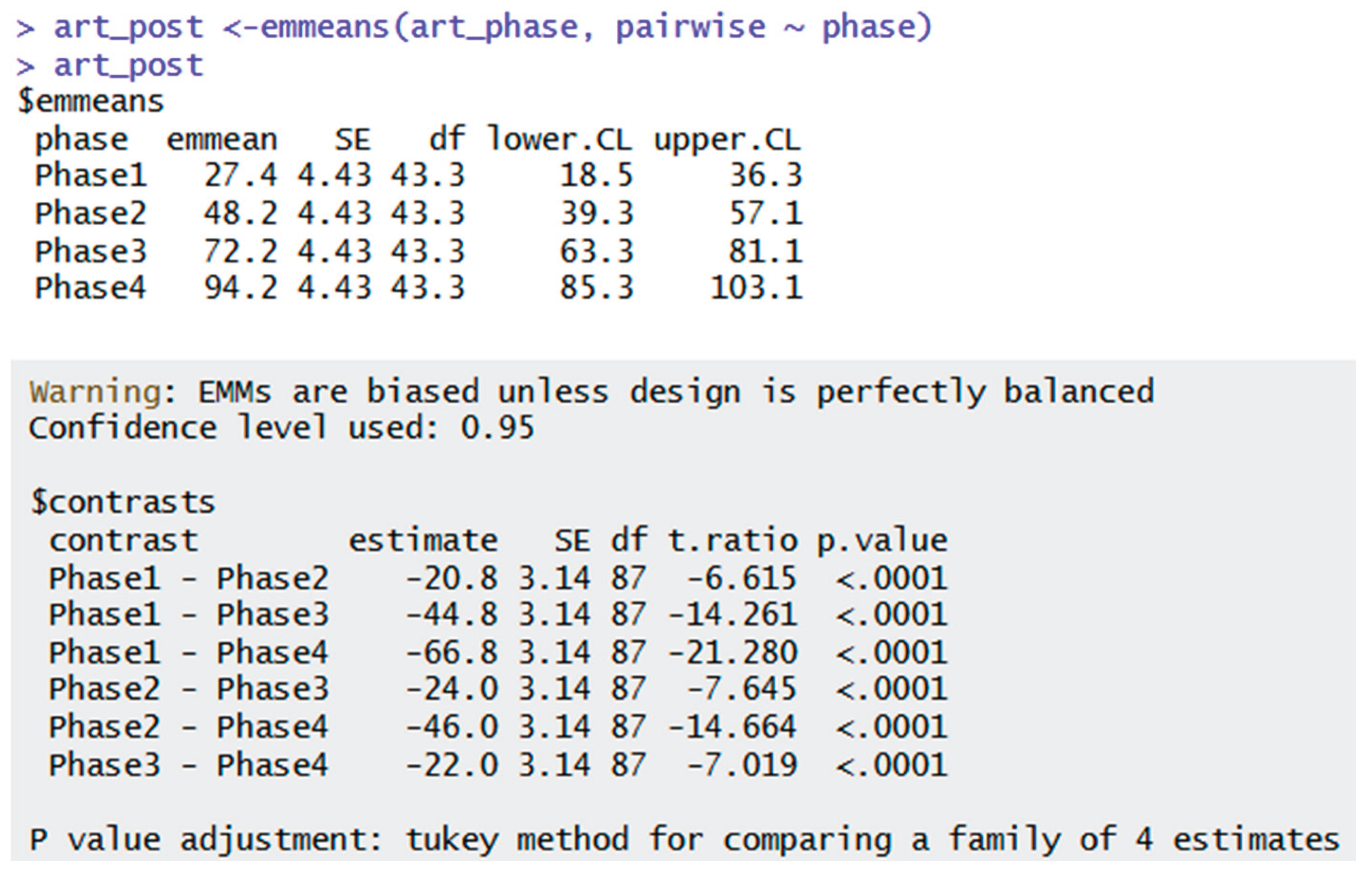
As shown below, the Tukey adjustment is the default for pairwise comparisons. As aforementioned, other post hoc tests may be chosen in emmeans depending on the user’s preference and objective.
Figure 18.
Post hoc tests for ANOVA of aligned rank transformed data.
Discussion
R offers several options for one-way RMA analysis. In this tutorial, the rstatix package was used as it is a comprehensive package for parametric and nonparametric options. It offers descriptive statistics, parametric and nonparametric RMA, effect sizes, and post hoc tests. The afex package also offers parametric RMA and effect sizes. However, another package such as datawizard may be used to get descriptive statistics, and emmeans may be used for post hoc tests. The WRS2 package offers robust and bootstrapped RMA and post hoc tests, although it does not offer descriptive statistics or an effect size. The ARTool package may be used in tandem with the effectsize and emmeans packages to offer effect sizes and post hoc tests respectively.
Limitations
While four options are shown for RMA in this paper, it is not a comprehensive list of packages for this method. Users are encouraged to explore other packages at their discretion. This method is included in this tutorial, as it naturally progresses from the paired t-test, as independent ANOVA naturally progresses from the independent t-test. That said, RMA is not taught in all introductory courses, and instructors may choose to include or omit as they see fit. Multilevel models are an option for violations of the assumptions of relatedness and incomplete data. As this content is meant for an introductory course, these are not included.
Conclusions
R offers several options for RMA analysis and visualization. The rstatix package offers the most comprehensive option for parametric and nonparametric analyses. The afex package is a good option for parametric analysis, while WRS2 and ARTool offer options for violated assumptions. Readers are encouraged to practice using these packages and explore others at their own discretion.
References
- Ben-Shachar, M., Lüdecke, D., & Makowski, D. (2020). effectsize: Estimation of effect size indices and standardized parameters. Journal of Open Source Software, 5(56), 2815. [CrossRef]
- Cohen, J. (1988). Statistical Power Analysis for the Behavioral Sciences (2nd ed.). Hillsdale, NJ: Lawrence Erlbaum Associates, Publishers.
- Ellis, P. D. (2017). The essential guide to effect sizes : statistical power, meta-analysis and the interpretation of research results. Cambridge University Press.
- Field, A. (2013). Discovering statistics using IBM SPSS statistics (4th ed.). Sage Publications.
- Field, A., Miles, J., & Field, Z. (2012). Discovering Statistics Using R. SAGE.
- Kassambara, A. (2025). rstatix: Pipe-friendly framework for basic statistical tests. R package version 0.7.2.
- Kay, M., Elkin, L., Higgins, J., & Wobbrock, J. (2025). ARTool: Aligned rank transformation for nonparametric factorial ANOVAs. [CrossRef]
- Lenth, R., & Piaskowski, J. (2025). Emmeans: Estimated marginal means, aka least-squares means. [CrossRef]
- Mair, P., & Wilcox, R. (2019). Robust statistical methods in R using the WRS2 package. Behavior Research Methods, 52. [CrossRef]
- Patil, I. (2021). Visualizations with statistical details: The 'ggstatsplot' approach. Journal of Open Source Software, 6(61), 3167. [CrossRef]
- Patil, I., Makowski, D., Ben-Shachar, M. S., Wiernik, B. M., Bacher, E., & Ludecke, D. (2022). datawizard: An R Package for Easy Data Preparation and Statistical Transformations. Journal of Open Source Software, 7(78), 4684. [CrossRef]
- Posit (2025). RStudio Desktop. Posit. https://posit.co/download/rstudio-desktop/.
- R Core Team (2025). R: A language and environment for statistical computing. R Foundation for Statistical Computing, Vienna, Austria. https://www.R-project.org/.
- Singmann H., Bolker B., Westfall J., Aust F., & Ben-Shachar, M. (2025). afex: Analysis of factorial experiments. R package version 1.5-0, https://github.com/singmann/afex.
- Wickham, H., Vaughan, D., & Girlich, M. (2024). tidyr: Tidy Messy Data [R package tidyr version 1.1.3] https://doi.org/10.32614/CRAN.package.tidyr. R package version 1.3.1. [CrossRef]
- Wobbrock, J. O., Findlater, L., Gergle, D., & Higgins, J. J. (2011). The aligned rank transform for nonparametric factorial analyses using only ANOVA procedures. Proceedings of the 2011 Annual Conference on Human Factors in Computing Systems - CHI ’11. [CrossRef]
Figure 14.
Robust one-way repeated measures ANOVA using WRS2.
Disclaimer/Publisher’s Note: The statements, opinions and data contained in all publications are solely those of the individual author(s) and contributor(s) and not of MDPI and/or the editor(s). MDPI and/or the editor(s) disclaim responsibility for any injury to people or property resulting from any ideas, methods, instructions or products referred to in the content. |
© 2026 by the authors. Licensee MDPI, Basel, Switzerland. This article is an open access article distributed under the terms and conditions of the Creative Commons Attribution (CC BY) license (http://creativecommons.org/licenses/by/4.0/).
Copyright: This open access article is published under a Creative Commons CC BY 4.0 license, which permit the free download, distribution, and reuse, provided that the author and preprint are cited in any reuse.


