
Submitted:
05 February 2026
Posted:
06 February 2026
Read the latest preprint version here
Abstract
Let $A\in\C^{d\times d}$ and let $W(A)$ denote its numerical range. For a bounded convex domain $\Omega\subset\C$ with $C^1$ boundary containing $\spec(A)$, consider the operator-valued boundary kernel \[ P_{\Omega}(\sigma,A)\;:=\;\Real\!\Bigl(n_{\Omega}(\sigma)\,(\sigma\Id-A)^{-1}\Bigr), \qquad \sigma\in\partial\Omega, \] where $n_{\Omega}(\sigma)$ is the outward unit normal at $\sigma$. For convex $\Omega$ with $W(A)\subset\Omega$ this kernel is strictly positive definite on $\partial\Omega$ and underlies boundary-integral functional calculi on convex domains. We analyze the opposite limiting regime $\Omega\downarrow W(A)$. Along any $C^1$ convex exhaustion $\Omega_\varepsilon\downarrow W(A)$, if $\sigma_\varepsilon\in\partial\Omega_\varepsilon$ approaches $\sigma_0\in\partial W(A)$ with convergent outward normals and $\sigma_0\notin\spec(A)$, then $\lambda_{\min}(P_{\Omega_\varepsilon}(\sigma_\varepsilon,A))\to 0$ and the corresponding min-eigenvectors converge (up to subsequences and phases) to the canonical subspace $(\sigma_0\Id-A)\mathcal M(n)$ determined by the maximal eigenspace of $H(n)=\Real(\overline{n}A)$. Quantitatively, we obtain two-sided bounds in terms of an explicit support-gap scalar, yielding a linear degeneracy rate under bounded-resolvent hypotheses and an explicit rate for outer offsets $W(A)+\varepsilon\mathbb{D}$. For normal matrices we compute the eigenvalues of $P_{\Omega}(\sigma,A)$ explicitly, showing that degeneracy may fail at spectral support points unless the supporting face contains multiple eigenvalues.
Keywords:
numerical range
; operator-valued Poisson kernel
; convex domains
; functional calculus
; boundary integral methods
1. Introduction
Let and denote its numerical range
It is a compact convex subset of (Toeplitz–Hausdorff theorem; see, e.g., [1,2]). A central open problem due to Crouzeix asks whether is a 2-spectral set for A, i.e.,
See [3,4] for the formulation and [5] for the best known universal constant .
Background and relation to the convex-domain functional calculus. Up to harmless normalization conventions, a recurring tool in the convex-domain approach of Delyon–Delyon and Crouzeix is the operator-valued boundary kernel
defined for a bounded convex domain with boundary containing , where is the outward unit normal at . This kernel appears in double-layer potential representations and boundary integral operators used to obtain functional calculus bounds on convex domains [4,5,6,7,8]. For convex with , positivity/coercivity of on encodes strict separation of supporting half-planes and serves as a key structural input in such estimates [7,8,9].
Motivation: loss of coercivity near . In applications and numerical implementations of boundary-integral calculi, one often approximates by convex supersets . It is therefore natural to ask whether coercivity of the pointwise kernel can remain uniform as . The results below show that this is impossible in general: even when the resolvent stays bounded (i.e. at non-spectral boundary points ), the smallest eigenvalue of must deteriorate at boundary points approaching in a fixed supporting direction.
What is new in this paper. The existing convex-domain literature primarily exploits positivity of (1.2) for fixed domains [4,7,8,9]. Here we analyze the complementary limiting regime in which shrinks to , and we make explicit the resulting loss of coercivity of the pointwise kernel. The analysis is driven by a congruence identity and by a scalar support gap , which admits a support-function interpretation in standard convex-geometry terminology.
- We prove a qualitative degeneracy theorem (Theorem 1): along any convex exhaustion , if approaches a non-spectral boundary point with convergent outward normals , then and the limiting min-eigenvector directions lie in , where is the maximal eigenspace of .
- We establish two-sided bounds for in terms of the support gap , yielding a linear degeneracy rate under bounded-resolvent hypotheses (Lemma 3 and Corollary 3), and compute explicitly for standard outer offsets (Proposition 2).
- Under a spectral-isolation hypothesis for , we obtain convergence of the entire near-kernel invariant subspace (spectral projector) along the exhaustion (Proposition 3).
- We analyze the contrasting spectral-support regime for normal matrices via an explicit eigenvalue formula for , showing that degeneracy may fail at a spectral support point unless the supporting face contains multiple eigenvalues (Proposition 4 and Examples 1–2).
Organization.Section 2 fixes notation and recalls support-function identities. Section 3 introduces , proves the key congruence identity, and establishes quantitative support-gap bounds together with a geometric interpretation of . Section 4 contains the degeneracy theorem, quantitative corollaries, subspace convergence, and explicit examples, followed by a brief discussion of open problems.
2. Preliminaries
We use the standard notation for disks:
Throughout, is fixed. For vectors we use . For matrices we use the induced operator norm . We write for the conjugate transpose and .
For a Hermitian matrix B, we write its eigenvalues in nondecreasing order as
and in nonincreasing order as . In particular, and .
Remark 1
(Spectrum is contained in the numerical range). One has . Indeed, if with , then . Consequently, implies for any open set .
2.1. Support Functions and the Hermitian Pencil
For unimodular (i.e. ), define the Hermitian matrix
We will later write (with ) for outward unit normals on ; in the support-function identities below and throughout, such an n simply plays the role of the unimodular direction .
Let denote its largest eigenvalue and let
denote the corresponding maximal eigenspace.
Lemma 1
(Support function of the numerical range). For every unimodular ,
Moreover, if is a unit eigenvector of associated with , then and
Proof.
For ,
Taking the maximum over yields (2.2) by Rayleigh–Ritz. If x is a maximizing unit vector, then attains the support functional in direction , hence lies on and satisfies the stated identity. □
2.2. Convex Domains with Boundary and Normals
We identify with in the usual way. Let be a bounded open convex set with boundary. Then for each there is a unique outward unit normal vector. This assumption is used only to guarantee that the outward unit normal exists and is unique at every boundary point, ensuring that is well-defined; no higher regularity (e.g. curvature bounds) is used. We represent the normal as a unimodular complex number with so that the supporting half-plane at is
Equivalently, by convexity one has and . Under the identification , the functional is the Euclidean inner product with the unit vector corresponding to n.
Definition 1
( convex exhaustion). A family is called a convex exhaustionof a compact convex set if:
- (i)
- each is a bounded open convex set with boundary;
- (ii)
- for ;
- (iii)
- for all ;
- (iv)
- .
Remark 2
(Subsequence selection for convergent normals). Let and be any sequence. Since each outward normal is unimodular, the sequence lies in a compact set. Hence there is always a subsequence (not relabeled) such that for some unimodular n. In particular, the normal convergence hypothesis in Theorem 1 can always be arranged by passing to a subsequence.
3. The Operator-Valued Poisson Kernel
Let be a bounded open convex set with boundary and assume . Then exists for all .
Definition 2
(Operator-valued Poisson kernel). For , define
3.1. A Congruence Identity
Lemma 2
(Congruence identity). Let and let be unimodular. Then
Proof.
Write . Then and . Using ,
Expanding gives (3.2). □
3.2. Support-Gap Bounds
For unimodular define the support gap
Lemma 3
(Support-gap characterization and quantitative bounds). Let , let , and let be unimodular. Set
(This notation emphasizes dependence on the prescribed direction n; when one has .) Then:
- (a)
- if and only if , and if and only if .
- (b)
- If , then is singular and
- (c)
- If , then
Proof.
Let and . By Lemma 2,
Since B is invertible, congruence by B preserves (semi)definiteness, so and . As Q is Hermitian with , this proves (a).
If , then is singular with , and by (a). For , . Writing ,
so , proving (b).
If , then and . For and , one has and hence ; thus
giving the lower bound in (3.3). For the upper bound, take y a unit eigenvector of Q for and set ; then
□
Remark 3
(Connection with the convex-domain Poisson kernel literature). Up to normalization conventions, is the operator-valued boundary kernel appearing in the Carl Neumann double-layer potential framework for convex domains; see, e.g., [7,8,9]. Lemma 3 isolates the dependence of on the scalar support gap .
3.3. Strict positivity when
Lemma 4
(Strict separation at a supporting line). Let be a bounded open convex set with boundary and let be compact. Fix and let be the outward unit normal. Then
Proof.
By (2.3), , hence . The continuous function attains its maximum on compact K, and this maximum is strictly negative. Rearranging yields the claim. □
Proposition 1
(Positivity of the Poisson kernel). Assume . Then for every ,
Proof.
Fix and set and . By Lemma 4 with and Lemma 1,
so . Now apply Lemma 3 (a). □
3.4. Geometric Meaning of the Support Gap and Offset Exhaustions
For a compact convex set and unimodular , define its support function
If is a bounded open convex set with boundary and has outward normal , then necessarily , i.e. the boundary point lies on the supporting line in direction n.
Lemma 5
(Support gap as a support-function difference). Let be a bounded open convex set with boundary and . Let . Then
In particular, measures the separation between the supporting line of in direction n and the corresponding supporting line of .
Proof.
Since n is the outward unit normal at , the supporting half-plane characterization implies for all , hence . By Lemma 1, . Combining gives the claim. □
Proposition 2
(Outer offsets: is explicit). Let be compact and convex and fix . Define the outer offset (outer parallel set)
Then for every unimodular ,
In particular, taking and , for any boundary point with outward normal (whenever defined) one has
Consequently, since implies and hence (Remark 1), Lemma 3 (c) yields
Proof.
Fix unimodular n. For any and with ,
so . On the other hand, choosing with and gives and
so . This proves the support-function identity and hence the displayed formula for follows from Lemma 5.
The final eigenvalue bounds are an immediate substitution of into (3.3). □
Remark 4
(Smoothness versus offsets). If K has flat faces, then is typically only (curvature may jump at transitions between translated faces and rounded arcs). Proposition 2 is therefore best viewed as a geometric model illustrating how the support gap scales with the outer distance parameter ε. For the purposes of Definition 1, one may replace by any convex domain with boundary whose support function differs from by a quantity comparable to ε; the same interpretation of δ then applies. For example, one may take Minkowski sums with a fixed smooth strictly convex unit ball (instead of ) or smooth the support function to obtain a genuine (indeed smooth) convex exhaustion with the same first-order support-gap scaling.
3.5. Hausdorff distance and support-function control of the support gap
For a nonempty compact set and , write
For nonempty compact sets , define the (Euclidean) Hausdorff distance
Lemma 6
(Hausdorff distance via support functions). Let be nonempty compact convex sets and let . Then
If moreover , then for all and hence
Proof.
For and a nonempty compact set K, the Minkowski sum
is the closed t-neighborhood of K, i.e. . Consequently,
For compact convex sets one has if and only if for all . (Indeed, the forward direction is immediate; conversely, if , a separating supporting line for the convex compact set N yields a unimodular n with , hence .)
Moreover, support functions add under Minkowski sums, and for ; hence
Therefore, is equivalent to for all , and similarly is equivalent to for all . Thus is the smallest t such that for all , i.e.
If , then , so the absolute value may be dropped, giving the second identity. □
Corollary 1
(Support gap bounded by the Hausdorff approximation error). Assume , and set
Then for every with outward normal ,
Consequently, since for , Lemma 3 (c) yields
Moreover, there exists such that
and for this point one has the two-sided estimate
Proof.
The identity is Lemma 5, and the bound follows from the definition of . The eigenvalue bounds are then immediate from Lemma 3 (c).
Finally, the function is continuous on the unit circle, so it attains its maximum at some unimodular . Choose such that ; then and the supporting line is a supporting line for at . Since is , the outward unit normal at is uniquely defined and equals , and hence
□
4. Degeneracy Along a Convex Exhaustion
4.1. Qualitative Degeneracy and Limiting Kernel Directions
Theorem 1
(Degeneracy of the Operator-Valued Poisson Kernel). Let and let be a convex exhaustion of (Definition 1). For , set
Fix any sequence and points such that
(After passing to a subsequence, the convergence is automatic; see Remark 2.) Assume . Let and .
Then:
- (1)
- (Vanishing) as .
- (2)
- (Limiting directions)If is any unit eigenvector of for , then every accumulation point of satisfies
- (3)
-
(One-dimensional case)If , then there exist phases such thatwhere v is any unit vector spanning .
Proof.
Set and , and define
Define also , , , .
Step 1: Congruence identities. By Lemma 2,
where .
Step 2: . Since is the outward normal at , the supporting half-plane property gives for all and hence for all . Passing to the limit yields for all . Because , equality holds at , so . Lemma 1 now gives
so is singular.
Step 3: in operator norm. Since , is invertible. Write
Then , so for large k, is invertible and
Therefore,
Step 4: and . Since are Hermitian, Weyl’s inequality yields
so . By (4.1) and Step 2,
Since is invertible, is singular, hence , proving (1). Moreover,
by Lemma 3 (b) (with ).
Step 5: Limiting eigenvectors. Let be unit min-eigenvectors: . Along a convergent subsequence, . Then
Since , this implies , proving (2).
Step 6: One-dimensional case. If , then , so the smallest eigenvalue of is simple. By the Davis–Kahan theorem for invariant subspaces (see [10]), the corresponding one-dimensional eigenspaces of converge to in gap metric, hence there exist phases such that , where spans . This gives (3). □
Remark 5
(Why is essential). The hypothesis ensures that remains bounded near , so is a finite Hermitian matrix. When , the resolvent diverges and the behavior of depends on the spectral geometry; see Proposition 4 below and Section 4.7.
Corollary 2
(Global coercivity collapse along a convex exhaustion). Assume that A is not a scalar multiple of the identity (equivalently, is not a singleton). Let be a convex exhaustion of and define the global coercivity constant
Then
In particular, there do not exist and such that for all and all .
Proof.
Since A is not scalar, the compact convex set contains more than one point, hence is infinite, whereas is finite. Choose .
Fix any sequence . We claim that . Indeed, if not, then there exist and a subsequence (not relabeled) such that for all k, hence the open ball is contained in for all k. Taking closures and intersecting over k yields , contradicting .
Therefore we may choose with . By compactness of the unit circle, after passing to a subsequence we have for some unimodular n. Theorem 1 then gives
Since , it follows that . □
4.2. Quantitative Degeneracy Rate
Corollary 3
(Linear rate in terms of the support gap). In the setting of Theorem 1, define
Then for each k and . Moreover, for all sufficiently large k,
In particular, .
Proof.
Since and with normal , Lemma 4 and Lemma 1 imply , so .
As and , . Also in operator norm, hence . By Step 2 in the proof of Theorem 1, , so .
Set and . Since and is invertible, for large k one has and . Applying Lemma 3 (c) to gives
and the stated constants follow. □
4.3. Convergence of the Near-Kernel Subspace
Proposition 3
(Convergence of the near-kernel spectral projector). Assume the setting of Theorem 1 and set . Assume that is isolated with multiplicity m, i.e.
Let
be the orthogonal projector onto .
For each k, let and let be the orthogonal projector onto the direct sum of the eigenspaces of corresponding to its m smallest eigenvalues. Then as .
Moreover, writing , one has the explicit spectral-gap bound
and consequently, for all sufficiently large k,
Proof.
By Lemma 2 and Step 2 of Theorem 1,
The eigenvalues of are 0 with multiplicity m and at least on , so .
Using the Courant–Fischer characterization with the change of variables , one obtains for every j
Taking gives (4.4).
Next, Theorem 1 gives . Since has an isolated cluster of m eigenvalues at 0 separated by the gap , the Davis–Kahan theorem for invariant subspaces [10] yields (4.5), and hence . □
4.4. The Spectral-Support Regime for Normal Matrices
Proposition 4
(Normal matrices: explicit eigenvalues near a spectral support point). Let A be normal with eigenvalues (listed with algebraic multiplicity). Fix and unimodular . Then
is unitarily diagonalizable and its eigenvalues are the scalars
Now fix and let
Let and unimodular satisfy
Write . Then:
- (i)
- For every ,
- (ii)
-
For every one has theexactidentityIn particular, if there exists such thatthen for every .
- (iii)
-
Assume in addition that n is a supporting direction for at , i.e.Then for every ,and if and only if lies on the same supporting line . If moreover (4.7) holds (so that all for ), thenwhich is strictly positive if and only if no eigenvalue lies on the supporting line .
Proof.
Since A is normal, for some unitary U, hence
Therefore,
which proves (4.6). The limit in (i) follows by continuity of the map when . For (ii), if then
and (4.7) implies .
Finally, (4.8) implies for all j, giving the nonnegativity (and the characterization of equality) in (iii). If additionally (4.7) holds, then for all while for , so for large k the minimum eigenvalue is attained among indices , yielding the stated limit and positivity criterion. □
Example 1
(Nondegeneracy at a spectral support point). Let , so . Take with and . Then
so as . Thus the smallest eigenvalue doesnotdegenerate when the limiting support point is spectral and unique on the support face.
Example 2
(Degeneracy at a spectral point with a flat support face). Let and take , . Then
so . Here the supporting functional is maximized by more than one eigenvalue, and degeneracy persists at .
4.5. A fully explicit example: a nilpotent Jordan block
Example 3
(Exact Poisson kernel and exact degeneracy rate for a disk exhaustion). Let
Then . For , let and choose . The outward normal at σ is and
Hence
whose eigenvalues are . In particular,
so the degeneracy islinearas .
Moreover, a min-eigenvector is (independent of r). For the support direction ,
At ,
in agreement with Theorem 1.
4.6. Numerical Experiments
This section provides numerical illustrations of: (i) the linear degeneracy predicted by Corollary 3 (and, in offset form, Proposition 2), (ii) the global coercivity collapse of Corollary 2, and (iii) the contrasting behavior at spectral support points for normal matrices (Proposition 4 and Examples 1–2).
Sampling model for an “outer offset” exhaustion. Fix a unimodular direction . Let and let be a unit vector in the maximal eigenspace of (Lemma 1). The corresponding numerical-range support point is
For we define the offset boundary point
Then , so the support gap equals (cf. Proposition 2). Moreover, , hence (because ; Remark 1), so the resolvent is well-defined.
We evaluate the pointwise kernel
and track as . In the generic (bounded-resolvent) regime , Corollary 3 predicts the linear scaling and convergence of min-eigenvectors to (Theorem 1).
Experiment 1: exact linear rate for the nilpotent Jordan block. We revisit Example 3 with and the disk exhaustion , . Writing , one has the exact formula , hence linear degeneracy as . Figure 1 compares the computed smallest eigenvalue to the exact expression.
Experiment 2: generic nonnormal matrix—linear degeneracy and eigenvector convergence. We generate a fixed random complex matrix (seeded for reproducibility), fix one direction , and form as above. Figure 2 shows against on a log–log scale, together with a reference line; the observed slope is on the plotted range. Figure 3 tracks the distance of a min-eigenvector of to the predicted limiting subspace , quantified by where is the orthogonal projector onto (consistent with Theorem 1).
Experiment 3: approximate global coercivity collapse. For the same A we approximate the global coercivity constant
by sampling a fine grid of directions and using the offset model . Figure 4 plots the sampled minimum versus , illustrating the collapse asserted by Corollary 2. (Here the offset model has , so Corollary 1 also predicts that uniform coercivity cannot persist as .)
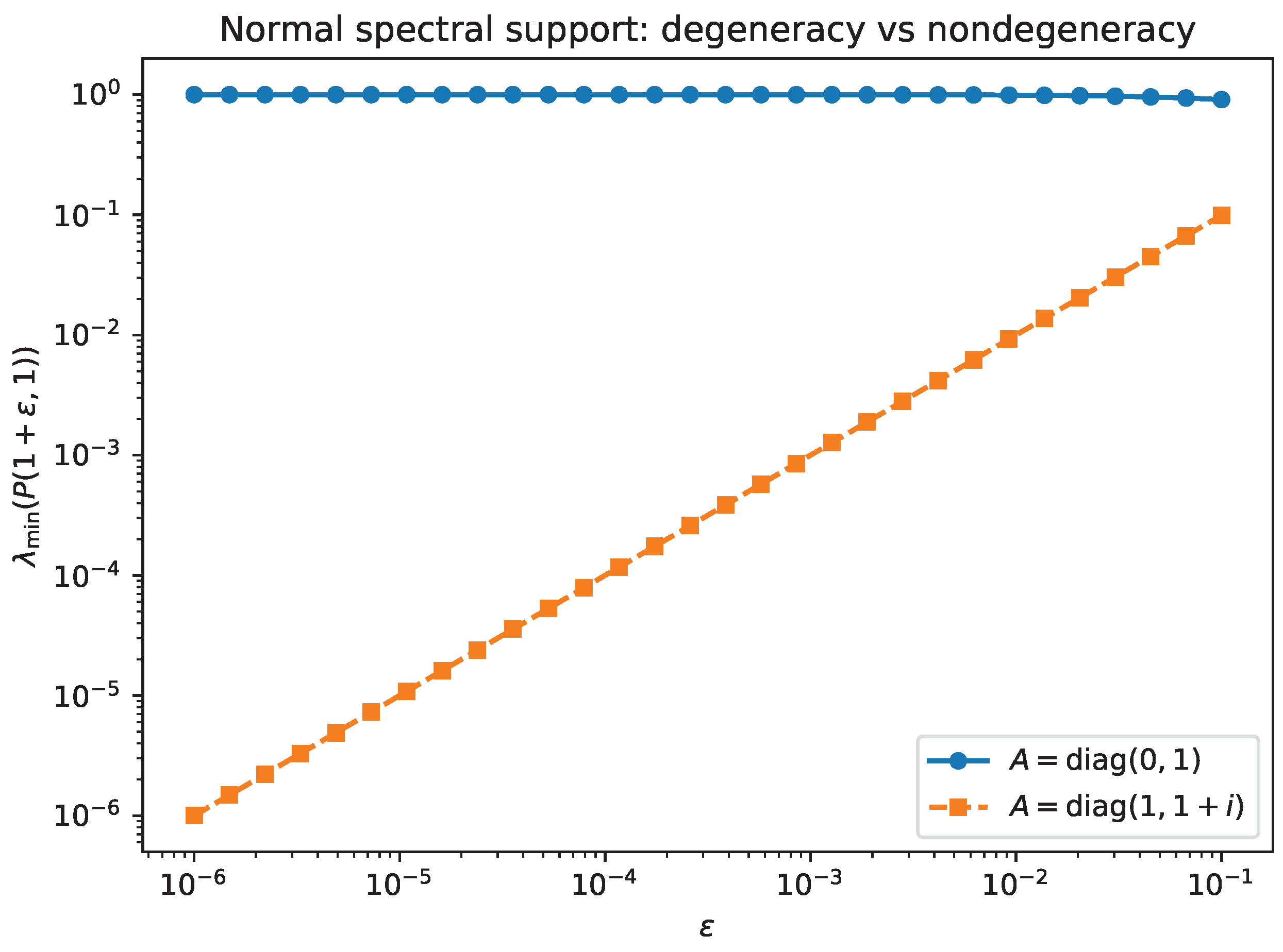
Experiment 4: normal matrices at spectral support points. We reproduce the contrasting behavior in Examples 1–2 by evaluating for two diagonal (hence normal) matrices: and . Figure 5 shows that the former remains bounded away from 0 as , while the latter degenerates linearly, consistent with Proposition 4.
Reproducibility. All figures are generated by the accompanying scripts poisson_utils.py and run_numerical_experiments.py, which require only NumPy and Matplotlib and save PDF figures into a figs/ folder.
4.7. Discussion and Open Problems: the Nonnormal Spectral-Support Regime
Remark 6
(Beyond the normal case at spectral support points). Theorem 1 treats the bounded-resolvent regime , while Proposition 4 gives a complete description of what can happen at a spectral support point fornormalmatrices.
Fornonnormalmatrices, the regime appears substantially more delicate: the resolvent typically diverges as , and the interplay between (i) the approach geometry along , (ii) the supporting direction n, and (iii) the Jordan/pseudospectral behavior of A near can produce several qualitatively different limits for .
Natural questions suggested by the present results include:
- Can one classify (or even bound) the possible asymptotic behavior of as , in terms of the local spectral data of A (e.g. Jordan structure) and the support direction n?
- In analogy with Proposition 4, is there a purely geometric/spectral criterion characterizing when degeneracy must occur at a spectral support point for a general (possibly defective) A?
- How do these boundary effects interact with quantitative constants in boundary-integral functional calculi and with conditioning of numerical schemes based on domain approximations ?
We leave these questions for future work.
References
- Toeplitz, O. Das algebraische Analogon zu einem Satze von Fejér. Math. Z 1918, 2(no. 1–2), 187–197. [Google Scholar] [CrossRef]
- Hausdorff, F. Der Wertevorrat einer Bilinearform. Math. Z 1919, 3(no. 1), 314–316. [Google Scholar] [CrossRef]
- Crouzeix, M. Bounds for analytical functions of matrices. Integral Equations Operator Theory 2004, 48, 461–477. [Google Scholar] [CrossRef]
- Crouzeix, M. Numerical range and functional calculus in Hilbert space. J. Funct. Anal. 2007, 244(no. 2), 668–690. [Google Scholar] [CrossRef]
- Crouzeix, M.; Palencia, C. The numerical range is a (1+2)-spectral set. SIAM J. Matrix Anal. Appl. 2017, 38(no. 2), 649–655. [Google Scholar] [CrossRef]
- Delyon, B.; Delyon, F. Generalization of von Neumann’s spectral sets and integral representation of operators. Bull. Soc. Math. France 1999, 127(no. 1), 25–41. [Google Scholar] [CrossRef]
- Badea, C.; Crouzeix, M.; Delyon, B. Convex domains and K-spectral sets. Math. Z 2006, 252(no. 2), 345–365. [Google Scholar] [CrossRef]
- Schwenninger, F. L.; de Vries, J. The double-layer potential for spectral constants revisited. Integr. Equ. Oper. Theory 2025, 97 13. [Google Scholar] [CrossRef] [PubMed]
- Crouzeix, M.; Greenbaum, A. Spectral Sets: Numerical Range and Beyond. SIAM J. Matrix Anal. Appl. 2019, 40(no. 3), 1087–1101. [Google Scholar] [CrossRef]
- Davis, C.; Kahan, W. M. The rotation of eigenvectors by a perturbation. III. SIAM J. Numer. Anal. 1970, 7, 1–46. [Google Scholar] [CrossRef]
Figure 1.
Nilpotent Jordan block (Example 3): log–log plot of versus , showing the predicted linear scaling.
Figure 1.
Nilpotent Jordan block (Example 3): log–log plot of versus , showing the predicted linear scaling.
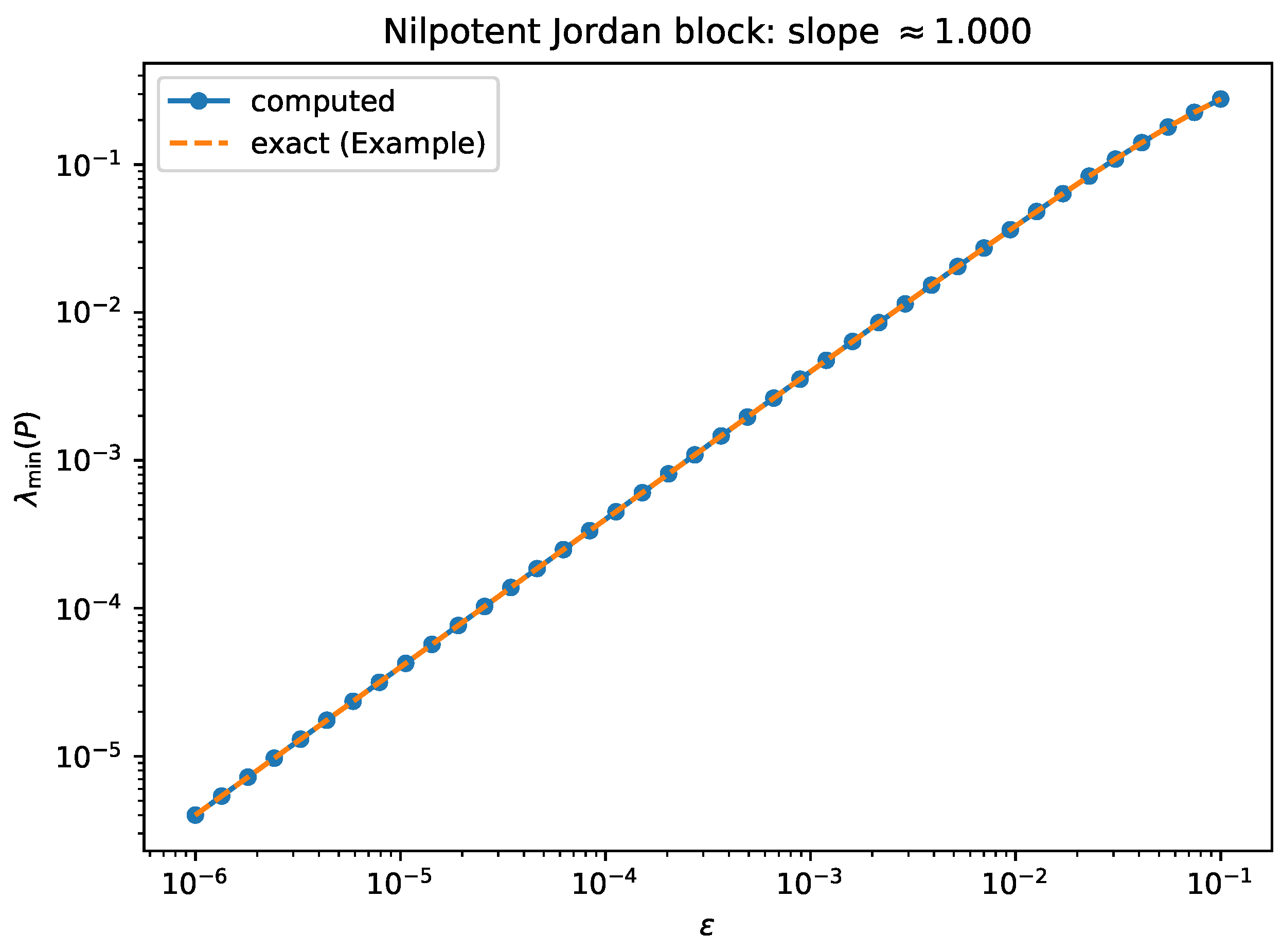
Figure 2.
Random nonnormal (fixed seed), fixed direction n: scales linearly in (Corollary 3).
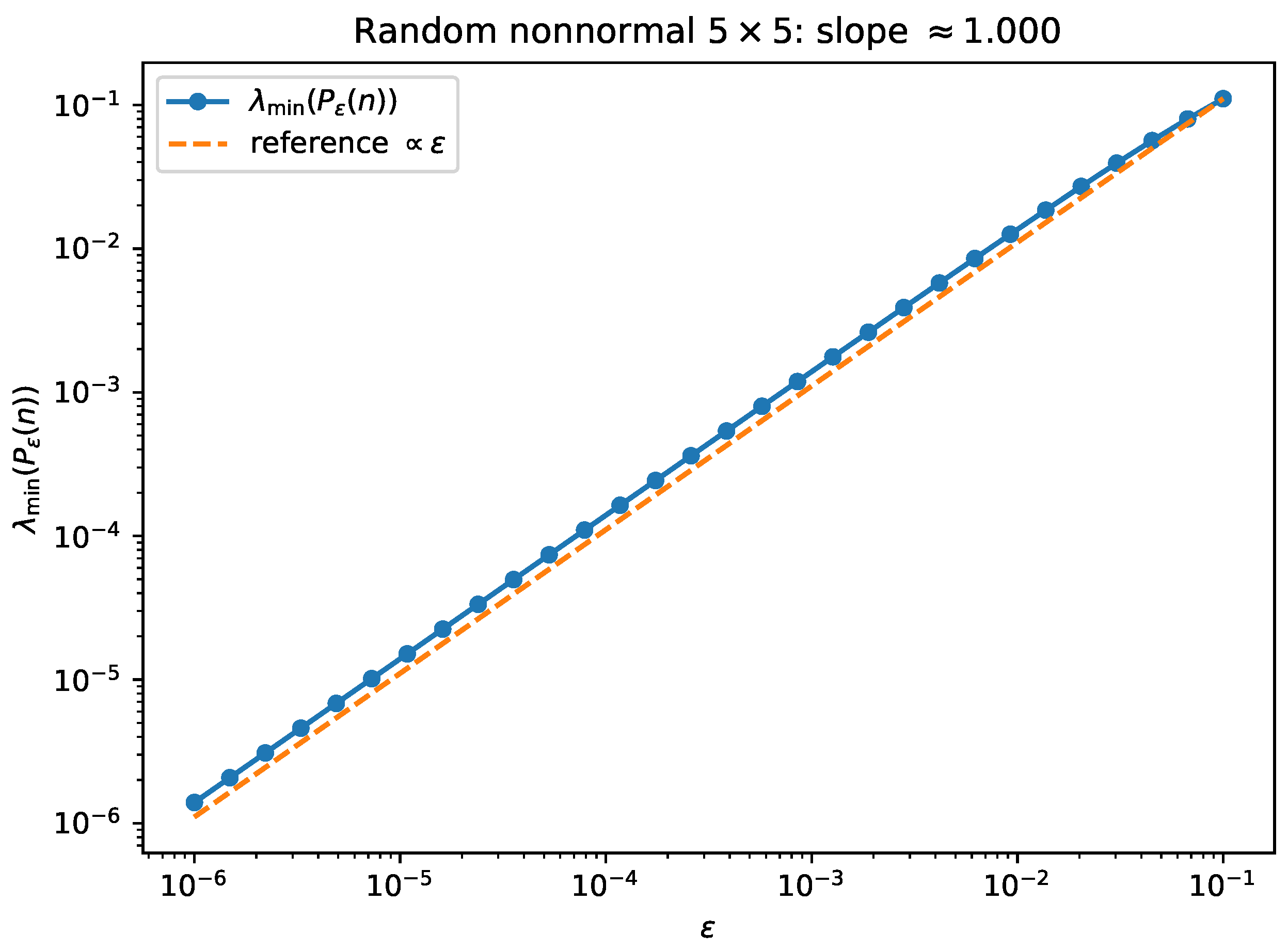
Figure 3.
Same setup as Figure 2: the min-eigenvector direction converges to as (Theorem 1). The plotted “gap” is .
Figure 3.
Same setup as Figure 2: the min-eigenvector direction converges to as (Theorem 1). The plotted “gap” is .
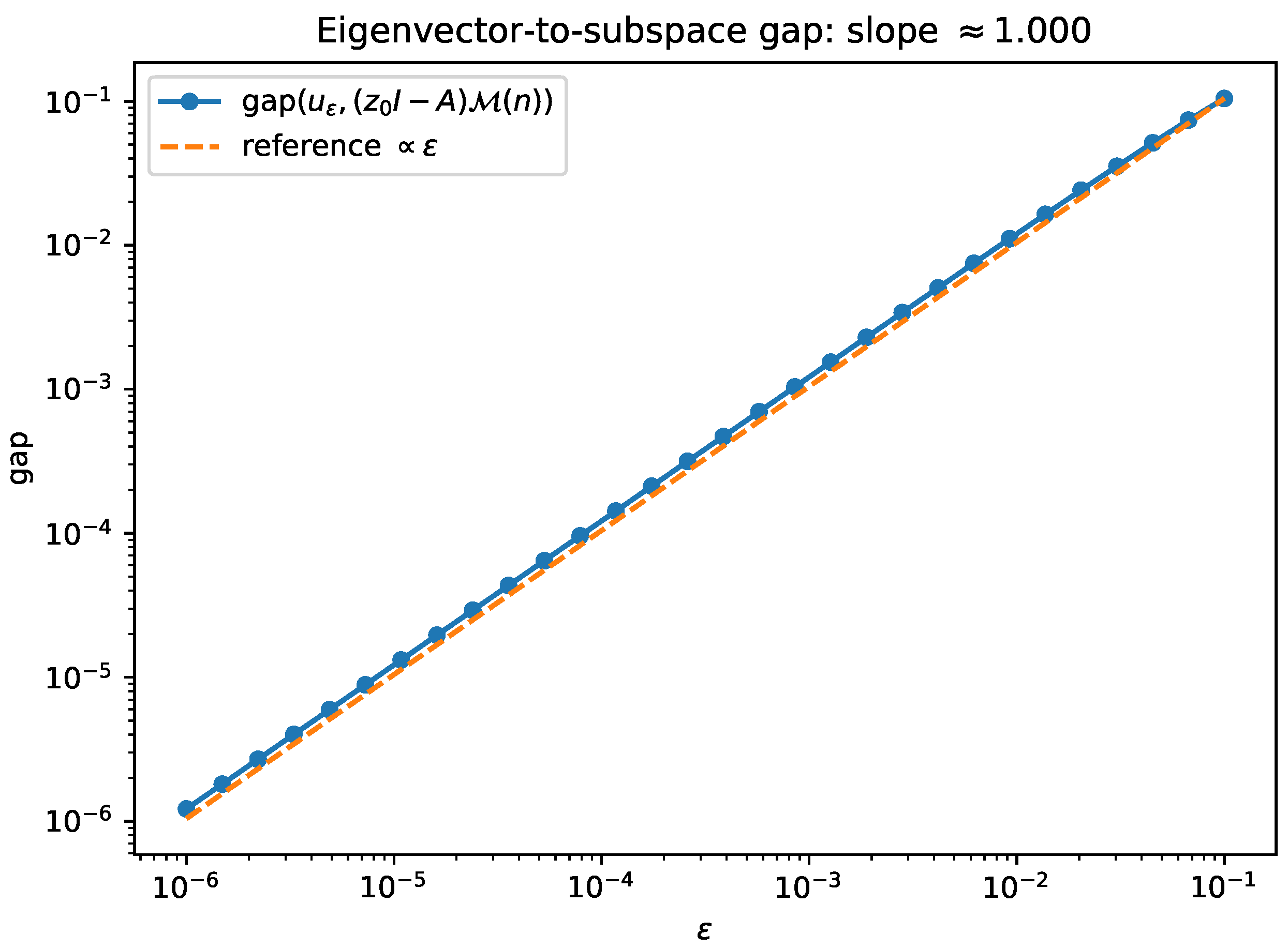
Figure 4.
Approximate global coercivity constant computed by sampling directions and using the offset model . The minimum over directions tends to 0 with (Corollary 2).
Figure 4.
Approximate global coercivity constant computed by sampling directions and using the offset model . The minimum over directions tends to 0 with (Corollary 2).
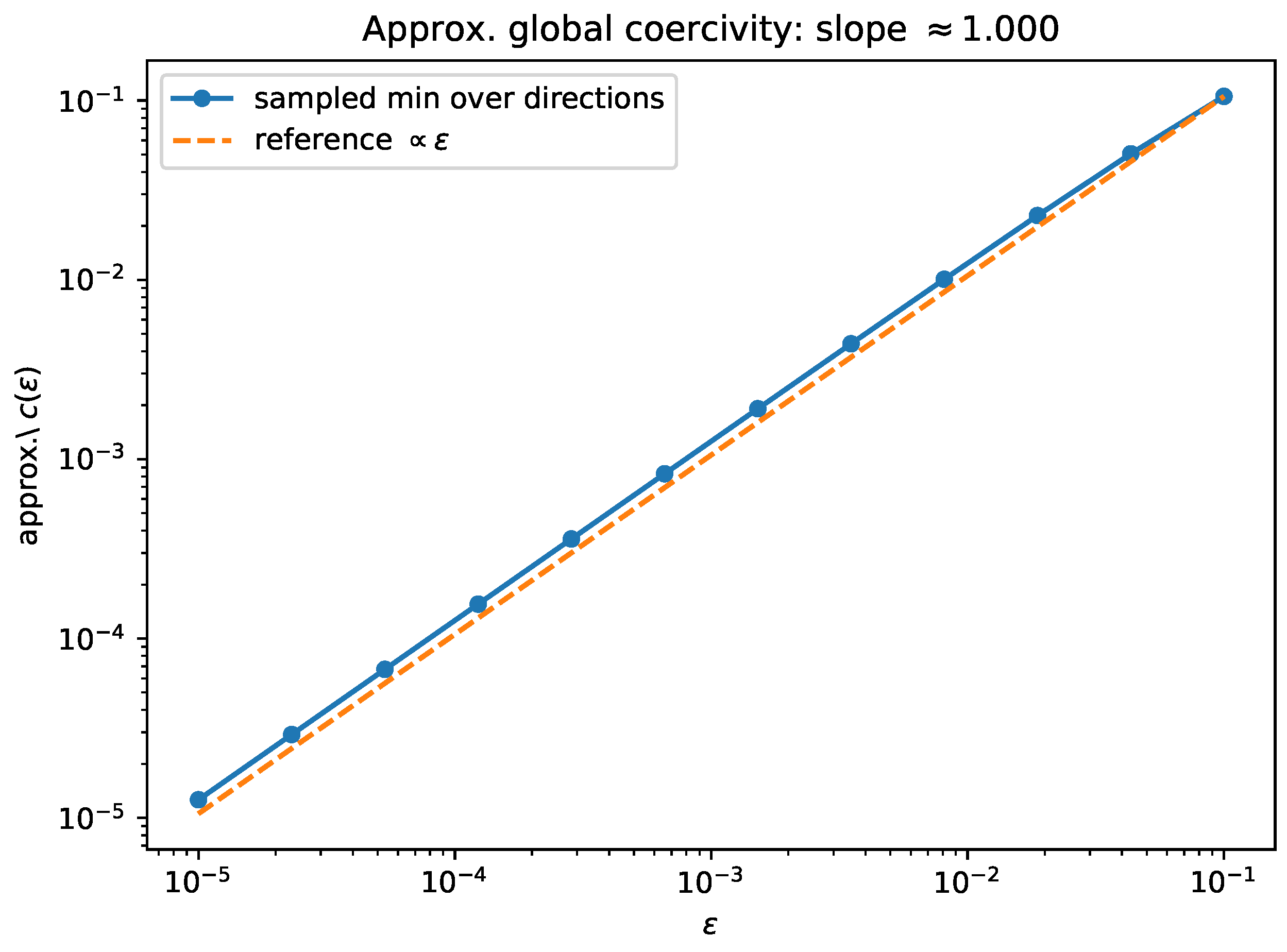
Figure 5.
Normal matrices at a spectral support point: nondegeneracy for versus linear degeneracy for , consistent with Proposition 4.
Figure 5.
Normal matrices at a spectral support point: nondegeneracy for versus linear degeneracy for , consistent with Proposition 4.
Disclaimer/Publisher’s Note: The statements, opinions and data contained in all publications are solely those of the individual author(s) and contributor(s) and not of MDPI and/or the editor(s). MDPI and/or the editor(s) disclaim responsibility for any injury to people or property resulting from any ideas, methods, instructions or products referred to in the content. |
© 2026 by the authors. Licensee MDPI, Basel, Switzerland. This article is an open access article distributed under the terms and conditions of the Creative Commons Attribution (CC BY) license (http://creativecommons.org/licenses/by/4.0/).
Copyright: This open access article is published under a Creative Commons CC BY 4.0 license, which permit the free download, distribution, and reuse, provided that the author and preprint are cited in any reuse.


