
Submitted:
06 February 2026
Posted:
06 February 2026
You are already at the latest version
Abstract
This paper features an empirical evaluation of Yang and Zhang’s (2000) short-cut method for calculating drift-independent realised volatility, based on high, low, open, and close prices using a historical time series. They suggest that this method is unbiased in the continuous limit, independent of the drift, and consistent when faced with opening price jumps. Souto and Moradi (2024) published Python script to implement this method and claimed that this was the first open-source code made available, that automates its estimation from high-frequency intraday stock data. We convert their code to R script and undertake an evaluation of the method using high-frequency hourly data on Bitcoin, originally sourced from Binance, for a period from January 1, 2018, to May 29, 2025. The method is benchmarked against the Bipower variation method of Barndorff-Nielsen and Shephard (2004a, 2004b). The ordinary least squares regression analysis reveals a close relationship between the methods. We further explore the persistence of volatility estimates by regressing the absolute values of daily Bitcoin returns on lags of themselves. The results suggest significant persistence out to seven daily lags. This finding supports the range enhanced GARCH model for modelling cryptocurrencies of Fiszeder et al. (2024). (The R code developed is attached in the Appendix).
Keywords:
short-cut volatility estimates
; Yang and Zhang
; realised Bipower covariance
; R code
1. Introduction
An empirical assessment of the Yang and Zhang (2000) short-cut method for calculating drift-independent realised volatility (RV) is performed using a historical time series of high, low, open, and close prices. The open-source Python script of Souto and Moradi (2024) is converted into R code and implemented in RStudio.
The Yang and Zhang (YZ) estimator utilises more information: unlike traditional methods that primarily rely on closing prices (e.g., close-to-close volatility), this estimator incorporates daily high, low, open, and close prices. It is drift-independent, and thus it is suggested that the estimator provides a more robust measure of volatility. It is designed to account for “opening price jumps” and provides an efficient and precise volatility estimates given the available data.
2. Literature Review
2.1. Evolution of Range-Based Volatility Estimators
The quest for more efficient volatility measures than those provided by daily squared returns or close-to-close estimators has a long history in financial econometrics. Early breakthroughs by Parkinson (1980) demonstrated that the high-low price range contains significantly more information about volatility than closing prices alone. This was further refined by Garman and Klass (1980), who incorporated opening and closing prices to create a more efficient estimator, though their model assumed a zero-drift process.
A major challenge in this field was developing an estimator that remained robust in the presence of both drift and "opening price jumps"—the gaps that occur between a previous day's close and the current day's open. Rogers and Satchell (1991) introduced an estimator () that was notably drift-independent, providing a more reliable measure when the underlying asset followed a geometric Brownian motion with non-zero drift. However, even this measure did not fully account for the volatility generated by overnight price gaps.
The synthesis of these approaches culminated in the Yang and Zhang (2000) estimator, which combines the overnight (close-to-open) volatility, the open-to-close volatility, and the Rogers-Satchell range-based estimator. By utilizing a weighting factor ($k$) to minimize variance, the Yang-Zhang method provides a measure that is theoretically unbiased in the continuous limit and independent of drift. Recent empirical work by Korkusuz et al. (2023) has begun to re-evaluate these extreme range estimators in the context of G7 stock markets, suggesting they may offer superior forecasting capabilities over traditional realized volatility measures
2.2. High-Frequency Data and the Bipower Variation Benchmark
While range-based "shortcuts" like the Yang-Zhang method rely on daily OHLC data, a parallel branch of literature has focused on the use of high-frequency intraday data to construct "realised" measures of volatility. This approach is predicated on the idea that summing squared returns over very short intervals—such as the hourly data used in this study—captures intraday dynamics and reduces the "noise" associated with end-of-day measures. However, simple realised volatility (RV) measures are often biased by market microstructure noise, such as bid-ask bounces and trading pauses.
The Realised Bipower Covariance (rBPCov) method, introduced by Barndorff-Nielsen and Shephard (2004a, 2004b), emerged as a robust solution to these frictions. Unlike standard quadratic variation methods that aggregate both continuous price movements and discrete "jumps," the rBPCov specifically targets and estimates the quadratic covariation of the continuous component of the price process. By utilizing products of absolute returns over adjacent high-frequency intervals, this method remains "robust to jumps," making it a preferred benchmark for evaluating the accuracy of other volatility estimators.
In the context of the 24/7 cryptocurrency market, where "jumps" are a frequent driver of fat-tailed distributions, the distinction between continuous and jump-driven volatility is critical. As noted in the development of the "highfrequency" R package by Boudt et al. (2022), the ability to isolate these components is essential for precise econometric analysis. This paper utilizes the rBPCov as a "gold standard" to test whether the computationally simpler Yang-Zhang shortcut can effectively capture the same volatility dynamics without the need for high-frequency data infrastructure.
Some of the benefits in contrast to daily, or lower frequency data, include the capturing of intraday dynamics. In an intraday sample you have more observations which should improve accuracy, and the estimates should be less noisy. The method should improve forecasting accuracy and pick up the impact of news events leading to changes in volatility more readily than end-of-day measures.
On the other hand, realised measures may be more susceptible to market microstructure noise such as bid-ask bounce, discrete price quotes, trading pauses etc. So, simply summing squared returns at the highest possible frequency can lead to biased estimates due to these frictions.
We required a benchmark to assess the effectiveness of the Yang and Zhang (2000) method, so we choose the Realised Bipower Covariance (rBPCov) method, introduced by Barndorff-Nielsen and Shephard in (2004a). This is regarded as being the preferred method for calculating realised volatility. This procedure has several advantages: it is robust to “jumps” in asset prices. Standard realised covariance methods estimate the total quadratic covariation of asset prices (which includes both the continuous diffusion component and any jump components), rBPCov specifically targets and consistently estimates the quadratic covariation of the continuous component of the price process. The core idea behind Bipower variation (BPV) is to utilise products of absolute returns (or sums of absolute returns) over adjacent high-frequency intervals.
2.3. Volatility Persistence and the Taylor Effect
A fundamental characteristic of financial time series is that while returns themselves are often close to unpredictable, the magnitude of those returns—volatility—exhibits significant clustering and persistence. This phenomenon was prominently described by Taylor (1986), who observed that the autocorrelations of absolute returns are typically much larger than those of squared returns. This empirical regularity, now known as the "Taylor Effect," suggests that absolute returns provide a more robust proxy for the underlying volatility process than the squared returns traditionally used in standard GARCH models.
Granger and Ding (1995) expanded on this by exploring the long-memory properties of absolute returns, arguing that they offer a more stable measure of risk over time. In the context of digital assets, Takaishi and Adachi (2018) confirmed the presence of the Taylor Effect in Bitcoin time series, noting that the persistence of volatility often displays unique daily seasonality and time-lag dependence.
This persistence is particularly relevant for the evaluation of the Yang-Zhang (2000) estimator. If volatility is persistent, an efficient "shortcut" estimator that captures the range-based dynamics of a single day should logically correlate with future volatility. Recent studies, such as Fiszeder et al. (2024), have leveraged these range-based insights to enhance GARCH models, demonstrating that incorporating range-based data—like the high and low prices used in this paper—leads to superior forecasting of Value at Risk and expected shortfall in cryptocurrency markets. By regressing absolute daily returns on multiple lags, this study explicitly tests whether the "Taylor Effect" holds for our specific Bitcoin sample, thereby situating the Yang-Zhang estimator within the broader framework of volatility forecasting.
2.4. Identification of Research Gaps
Despite the established theoretical advantages of the Yang-Zhang (YZ) estimator, its application in the rapidly evolving cryptocurrency landscape remains under-explored in several key dimensions. First, much of the foundational literature on range-based estimation was developed for traditional equity markets with set trading hours and discrete overnight gaps. In contrast, the 24/7 continuous trading nature of Bitcoin presents a unique environment where the "opening jump" is not a structural market closure gap but a result of arbitrary daily periodization. While recent studies (Korkusuz et al., 2023) have tested range estimators on G7 stock markets, there is a significant lack of empirical work that benchmarks the YZ "shortcut" against high-frequency measures like Realised Bipower Covariance specifically within the crypto-asset class.
Second, a notable "software-to-science" gap exists. While advanced volatility modeling is common in institutional finance, the tools to implement these specific range-based shortcuts have only recently become accessible in open-source environments. Souto and Moradi (2024) provided a vital contribution with their Python-based automation of the YZ method, but the academic and statistical community remains heavily reliant on the R ecosystem for reproducible econometric research. There is currently no widely documented R-based implementation that replicates these automated "shortcut" results for a 2020s-era Bitcoin dataset.
This paper addresses these gaps by:
- Methodological Bridging: Providing a direct empirical comparison between the daily YZ estimator and the high-frequency rBPCov benchmark in a continuous trading environment.
- Technological Contribution: Converting and validating the automated logic from Python into an R-based framework, ensuring that researchers in the R community can efficiently deploy these shortcuts.
- Temporal Relevance: Testing the validity of the "Taylor Effect" and volatility persistence using the most recent Bitcoin price dynamics, thereby updating the findings of earlier studies like Takaishi and Adachi (2018).
3. Materials and Methods
3.1. Data Set
The data used was Bitcoin historical data (2018-2025), in hourly observations, in US dollar terms (BTC/USDT), from January 1, 2018, to May 29, 2025, providing 64,823 datapoints (A feature of Bitcoin is that it trades 24 hours per day). The data was sourced from the Binance API and made available on Kaggle at the following webaddress:https://www.kaggle.com/datasets/novandraanugrah/bitcoin-historical-datasets-2018-2024?resource =download&select=btc_15m_data_2018_to_2025.csv.
Table 1 provides a descriptive summary of the Bitcoin hourly dataset converted into 2701 daily continuously compounded returns. The mean and median returns are positive at around 0.07 percent a day, there is very pronounced volatility, given that the standard deviation is 0.036 and the coefficient of variation is a massive 46.705. There is negative skewness of -1.1456 and very pronounced excess kurtosis of 17.089. A plot of the daily Bitcoin returns is provided in Figure 1.
3.2. Research Method
3.1.1. Yang-Zhang Estimator
The formula for the YZ volatility (variance) is given as
, (1)
where is the YZ daily volatility (variance), is the variance of open-to-close (OC) returns, is the variance of close-to-open (CO) returns (overnight returns), is the Rogers-Satchell (RS) volatility (variance) (Rogers and Satchell, 1991) and is a weighting factor. We take the logs of all the series: (log of open price on day ), (log of high price on day ), (log of low price on day ), and (log of close price on day ). The OC volatility () is a component that captures the volatility within the trading day. For days of data, assuming zero drift, is given by
, (2)
while the CO volatility () captures the over-night volatility. Again, assuming no drift, it is given by
. (3)
The RS volatility () estimator is drift-independent and robust to opening price jumps. Its average estimator is given by
. (4)
The weighting factor was derived by Yang and Zhang (2000) as the optimal factor that minimises the variance of their estimator. This is given by
,
where is the number of days in the estimation period.
For trading days, the YZ estimator for the daily variance can then be written as
, (5)
with the final YZ volatility is the square root of this variance: .
3.1.2. Barndorff-Nielsen and Shephard Realised Bipower Variance/Covariance
Barndorff-Nielsen and Shephard (2004a, 2004b) provide a recognised way for estimating the realised volatility of a set of high frequency (within the day) observations for a financial time-series that is robust to jumps. Their method provides a useful benchmark for testing the effectiveness of Yang-Zhang (2000) measure. We used the R library package ‘highfrequency’ by Boudt et al. (2022) to undertake the analysis on the Bitcoin data set and then uses the daily volatility estimates as a benchmark for testing the veracity of Yang-Zhang (2000) estimator.
Barndorff-Nielsen and Shephard (2004a, 2004b) proceed by letting be a d-dimensional vector of logarithmic asset prices. They assume that follows a general jump-diffusion semi-martingale process:
. (6)
In the Equation (6), is the -dimensional drift process, is a matrix-valued spot volatility process representing the instantaneous covariance of the continuous component, is a -dimensional standard Brownian motion, is a counting process representing the number of jumps up to time and are the jump sizes at the jump times.
The realised quadratic covariation over a period , based on intraday observations for returns (where ), is given by:
, (7)
where is the instantaneous covariance matrix of the continuous component, and the second term is the sum of squared jump sizes (the jump component of quadratic variation). This shows that estimates the total quadratic covariation, including jumps.
Barndorff-Nielsen and Shephard (2004a and 2004b) further demonstrate how to isolate the continuous component and how it is robust to jumps, via the realised Bipower covariation. Under regularity conditions, this realised Bipower covariation converges in probability to the integrated covariance of the continuous component. We estimate this benchmark measure, applied to the Bitcoin data, using the ‘highfrequency’ R package.
4. Results
Descriptive summaries of the YZ estimates of RV are shown in Table 2, together with the Barndorff-Nielsen and Shephard RV benchmark. It can be seen from Table 2 that the results of the two sets of estimations are very similar. The main difference is that that we programmed the YZ estimator in R in real numbers, whereas the estimates of RV in the ‘highfrequency’ R package are in percentage terms, so the values of the estimations differ by a factor of a 100. If we convert the YZ RV estimations into percentage terms, the mean YZ estimate of RV is 0.0159 whereas the mean estimate of the benchmark RV in the ‘highfrequency’ package is 0.00135. The coefficient of variation in the former is 2.304 and in the latter 2.346, the skewness is 12.963 for YZ and 13.347 for Barndorff-Nielsen and Shephard BPV, and finally the two values of the excess kurtosis are 252.83 and 272.57. Plots of the two different estimates of Bitcoin daily RV are shown in Figure 2.
Both distributions are right skewed, with have some extreme values in the right tail, and their means are greater than their medians. The Barndorff-Nielsen and Shephard Bi-power variation method, by construction, aims to isolate and estimate the continuous component of volatility, effectively “ignoring” or making itself robust to the presence of jumps. Since jumps are a major driver of fat tails in financial data, the theoretical and empirical distribution of the Bipower variation estimator (as an estimate of continuous volatility) tends to have lighter tails than the YZ method. The latter will still incorporate the impact of intraday jumps through its reliance on the high-low range, which makes its distribution appear to have fatter tails when jumps are present. This effect is accentuated by the fact that Bitcoin trades continuously, so all jumps are ‘within the day’.
We assessed the similarity between the two sets of estimates by standardising the two sets of estimates by dividing them by their standard deviation. We then ran an ordinary least squares (OLS) regression analysis of the benchmark BPV standardised estimates on the YZ standardised estimates. The results of the OLS regression reported in Table 3 suggest that there is a very close relationship between the two RV estimates. The slope coefficient is 0.979 which is significant at the 1% level. The R-squared is 0.956 and the F statistic is 62076, which is highly significant. This suggests that RV estimates based on high and low prices within the day, daily closing prices, and close to open prices, capture 95% of the BPV estimate of RV, at least in the case of this hourly sample of Bitcoin prices.
There are some peculiar features of Bitcoin, in that it is traded 24 hours per day, 365 days per year. This means that aspects of traditional asset markets, which feature opening/closing auctions or overnight gaps when the market is closed are not considerations. Bitcoin's continuous trading means that price discovery is constant and not subject to interruptions.
This suggests that volatility patterns might well be smoother and not display spikes at the open and the close that are a feature of traditional markets. However, the market is unregulated, and Bitcoin is traded on numerous independent exchanges worldwide. This creates highly fragmented liquidity, with different order books and varying prices across platforms at any given moment. On the other hand, this means that arbitrage can be continuous, which should promote price convergence. The dominance of retail investors may also mean that Bitcoin is over-exposed to news cycles, social media, pump-and-dump schemes, and the lack of circuit-breakers may account for Bitcoin’s relatively high volatility.
Granger and Ding (1995) mentioned the ‘Taylor effect’, in reference to Taylor (1986, Chapter 2), and the observation that persistence in volatility can be captured by the autocorrelation of the absolute return series. Takaishi and Adachi (2018) recently explored this feature of Bitcoin returns and reported that the Taylor effect is present in Bitcoin time series. They noted that: the power d that maximizes the autocorrelation is time-lag dependent, that exchange rate returns show a daily seasonality in the Taylor effect, and that they observed no evidence of seasonality. To further explore this matter, Table 4 reports an OLS regression of the absolute value of the daily Bitcoin return regressed on ten lags of itself.
It can be seen in Table 4 that seven of the ten lags are significant with six significant at the 1% level, and the Adjusted R-squared is 0.07. This suggests that Bitcoin volatility is very persistent.
5. Conclusions
We have explored the effectiveness of Yang and Zhang’s (2000) short-cut method for calculating drift-independent realised volatility, based on high, low, open, and close prices and applied the method to hourly Bitcoin prices. To benchmark the effectiveness of this approach we used the BPV method of calculating RV, of Barndorff-Nielson and Shephard (2004a, 2004b). The OLS results suggest the existence of a very close correspondence between the estimates produced by the two methods. Both the slope coefficient and the R squared of the regression are very close to 1, suggesting that investment analysts and portfolio risk modellers could use either measure, as estimates of volatility, in the case of Bitcoin, and that intraday observations do not confer a marked advantage, as daily observation from Yahoo finance that include, open, close, high and low prices, work equally well. This confirms the recent findings by Korkusuz et al. (2023) on G7 stock market indices,
We further explored the persistence in the volatility of daily Bitcoin prices using the absolute value of the return series and found significant evidence of persistence, in seven lags of daily absolute returns. Fiszeder et al. (2024) have demonstrated the superior forecasting performance of a GARCH model enhanced by range-based methods, as applied to Bitcoin, Ethereum Classic, Ethereum, and Litecoin and find that it forecasts variances, value at risk, and expected shortfall more accurately than the standard GARCH model. Our findings support this approach.
Supplementary Materials
The R Code used to implement the analysis is provided in the Appendix.
Author Contributions
Conceptualization, Allen, Chang, Ng, and Peiris.; methodology, Allen; software, Allen; validation, Allen, Chang, Ng, and Peiris.; formal analysis, Allen.; investigation, Allen; resources, Peiris.; data curation, Allen.; writing—original draft preparation, Allen.; writing—review and editing, Allen, Chang, Ng, and Peiris.; visualization, Allen.; project administration, Allen.; funding acquisition, Peiris. All authors have read and agreed to the published version of the manuscript.
Funding
This research was funded by the School of Mathematics and Statistics, The University of Sydney, and the personal funding account of Professor Shelton Peiris.
Informed Consent Statement
Not Applicable.
Data Availability Statement
The data was sourced from the Binance API and made available on Kaggle at the following webaddress:https://www.kaggle.com/datasets/novandraanugrah/bitcoin-historical-datasets-2018-2024?resource =download&select=btc_15m_data_2018_to_2025.csv.
Acknowledgments
The results of the analysis in this paper were presented at the 26th International Congress on Modelling and Simulation (MODSIM2025) held at the Adelaide Convention Centre from Sunday 30 November to 4 December 2025. The authors have reviewed and edited the output and take full responsibility for the content of this publication.
During: the preparation of this work, the authors used Gemini (a large language model built by Google) to assist with structural suggestions and language refinement. After using this tool, the authors reviewed and edited the content as needed and take full responsibility for the content of the publication.
Conflicts of Interest
The authors declare no conflicts of interest.
Abbreviations
The following abbreviations are used in this manuscript:
| MDPI | Multidisciplinary Digital Publishing Institute |
| DOAJ | Directory of open access journals |
| TLA | Three letter acronym |
| LD | Linear dichroism |
Appendix A
Appendix A.1 R Code used in the Analysis
#R Code to Run Yang and Zhang estimator 20 November 2025
# 1. Load Required Libraries
# The TTR package is needed for the volatility calculation.
# The xts package is the standard for financial time series in R.
# If these packages are not already installed, run:
# install.packages(c("TTR", "xts"))
library(TTR)
library(xts)
# 2. Load the Data
# Ensure the file path is correct for your environment.
file_path <- "~/conferences/MODSIM2025/RVPROXY/btc_1d_data_2018_to_2025.csv"
data_df <- read.csv(file_path, stringsAsFactors = FALSE)
# 3. Prepare the Data for Time Series Analysis (xts)
# a) Convert the 'Open.time' column to a proper Date/Time format.
# We will use this column as the time series index.
data_df$Open.time <- as.POSIXct(data_df$Open.time, format = "%Y-%m-%d %H:%M:%S", tz = "UTC")
# b) Select the necessary OHLC (Open, High, Low, Close) columns.
ohlc_data <- data_df[, c("Open", "High", "Low", "Close")]
# c) Create the xts time series object.
# xts is the preferred format for financial functions in R.
btc_xts <- xts(ohlc_data, order.by = data_df$Open.time)
# 4. Calculate Yang & Zhang Volatility
# The 'volatility' function from the TTR package is used.
# 'calc = "yang.zhang"' specifies the estimator.
# We set N=252 to annualize the daily volatility series (assuming 252 trading days). But 365 for Bitcoin.
#In this case because Bitcoin trades daily N=365.
# The result will be a daily annualized volatility series.
yz_volatility <- volatility(
OHLC = btc_xts,
calc = "yang.zhang",
N = 365,
mean.adj = TRUE # Standard setting for YZ volatility
)
# 5. Inspect the Results
# Print the start of the calculated daily volatility series.
cat("--- Head of Calculated Daily Yang & Zhang Volatility Series ---\n")
head(yz_volatility)
# 6. Plot the Volatility Series
# Plotting helps visualize the change in volatility over time.
plot(
yz_volatility,
main = "Annualized Daily Volatility (Yang & Zhang Estimator)",
ylab = "Annualized Volatility ($\\sigma$)",
major.format = "%Y-%m",
col = "blue"
)
# You can save the plot if needed:
# png("btc_yang_zhang_volatility.png", width = 800, height = 400)
# plot(yz_volatility, ...)
# dev.off()#R Code to Run Yang and Zhang estimator 20 November 2025
References
- Barndorff-Nielsen, O.E.; Shepherd, N. Power and bipower variation with stochastic volatility and jumps. Journal of Financial Econometrics 2004a, 2((1)), 1–37. [Google Scholar] [CrossRef]
- Barndorff-Nielsen, O.E.; Shepherd, N. Econometric analysis of realized covariation: High frequency based covariance, regression, and correlation in financial economics. Econometrica 2004b, 72(3), 885–925. Available online: https://www.jstor.org/stable/3598838. [CrossRef]
- Boudt, K.; Kleen, O.; Sjørup, E. Analyzing intraday financial data in R: The highfrequency package. Journal of Statistical Software 2022, 104(8), 1–36. [Google Scholar] [CrossRef]
- Fiszeder, P.; Małecka, M.; Molnár, P. Robust estimation of the range-based GARCH model: Forecasting volatility, value at risk and expected shortfall of cryptocurrencies. Economic Modelling 2024, 141, 106887. [Google Scholar] [CrossRef]
- Garman, M.B.; Klass, M.J. On the estimation of security price volatilities from historical data. Journal of Business 1980, 53, 67–78. [Google Scholar] [CrossRef]
- Granger, C.W.J.; Ding, Z. Some properties of absolute return: An alternative measure of risk. Annales d'Economie et de Statistique 1995, 40, 67–91. Available online: https://www.jstor.org/stable/20076016. [CrossRef]
- Korkusuz, B.; Kambouroudis, D.; McMillan, D.G. Do extreme range estimators improve realized volatility forecasts? Evidence from G7 Stock Markets. Finance Research Letters 2023, 55, 103992. [Google Scholar] [CrossRef]
- Parkinson, M. The extreme value method for estimating the variance of the rate of return. Journal of Business 1980, 53, 61–65. [Google Scholar] [CrossRef]
- Rogers, L.C.G.; Satchell, S.E. Estimating variance from high, low and closing prices. The Annals of Applied Probability 1991, 1(4), 504–512. Available online: https://www.jstor.org/stable/2959703. [CrossRef]
- Souto, H.G.; Moradi, A. Yang & Zhang’s realized volatility: Automated estimation in Python. Software Impacts 2024, 19, 100613. [Google Scholar] [CrossRef]
- Takaishi, T.; Adachi, T. Taylor effect in Bitcoin time series. Economics Letters 2018, 172, 5–7. [Google Scholar] [CrossRef]
- Taylor, S.J. Modelling Financial Time Series; Wiley: Chichester, 1986. [Google Scholar]
- Yang, D.; Zhang, Q. Drift-independent volatility estimation based on high, low, open, and close prices. The Journal of Business 2000, 73(3), 477–492. Available online: https://www.jstor.org/stable/10.1086/209650. [CrossRef]
Figure 1.
Plot of daily Bitcoin returns.
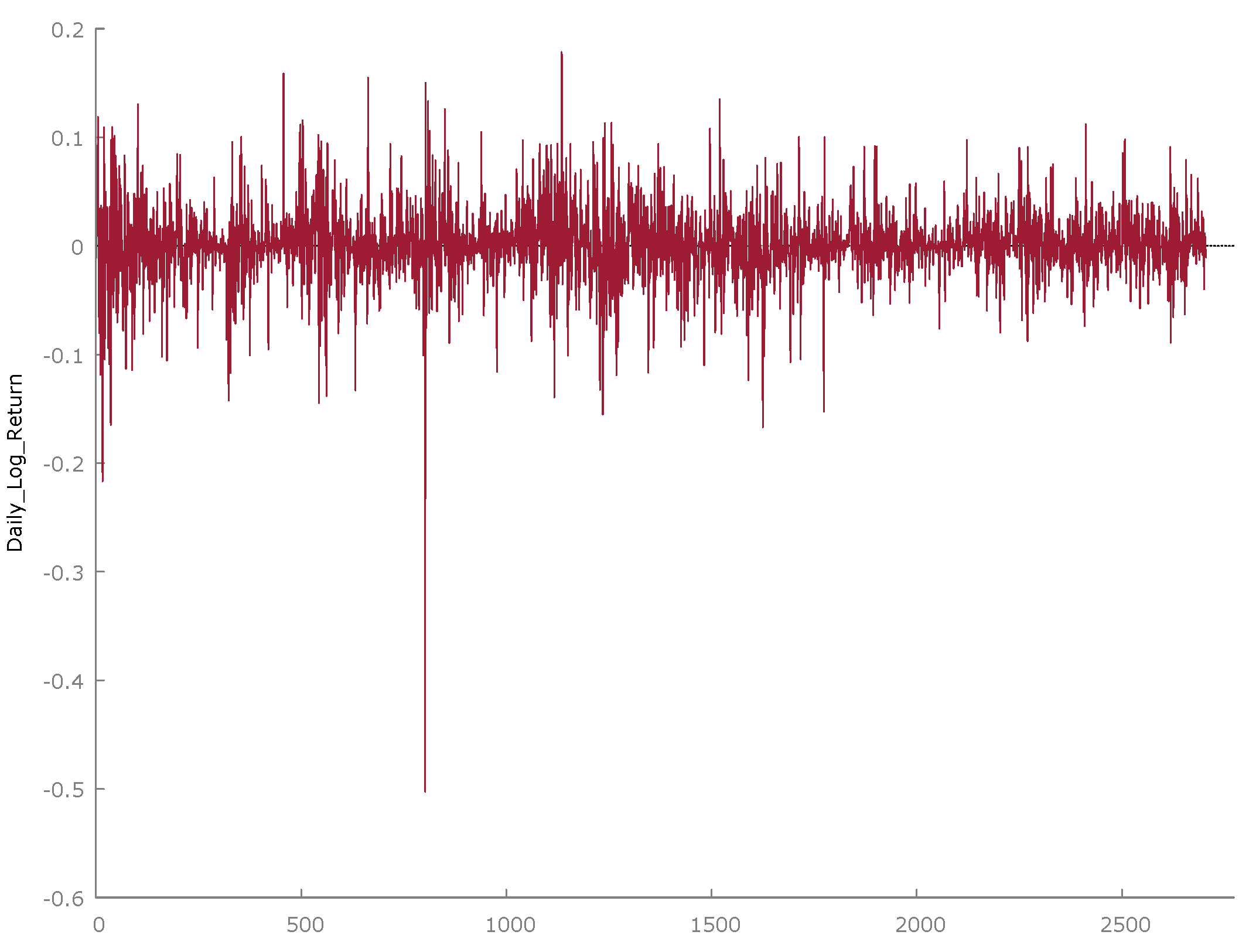
Figure 2.
Plots of YZ and BPV estimates of Bitcoin daily RV.
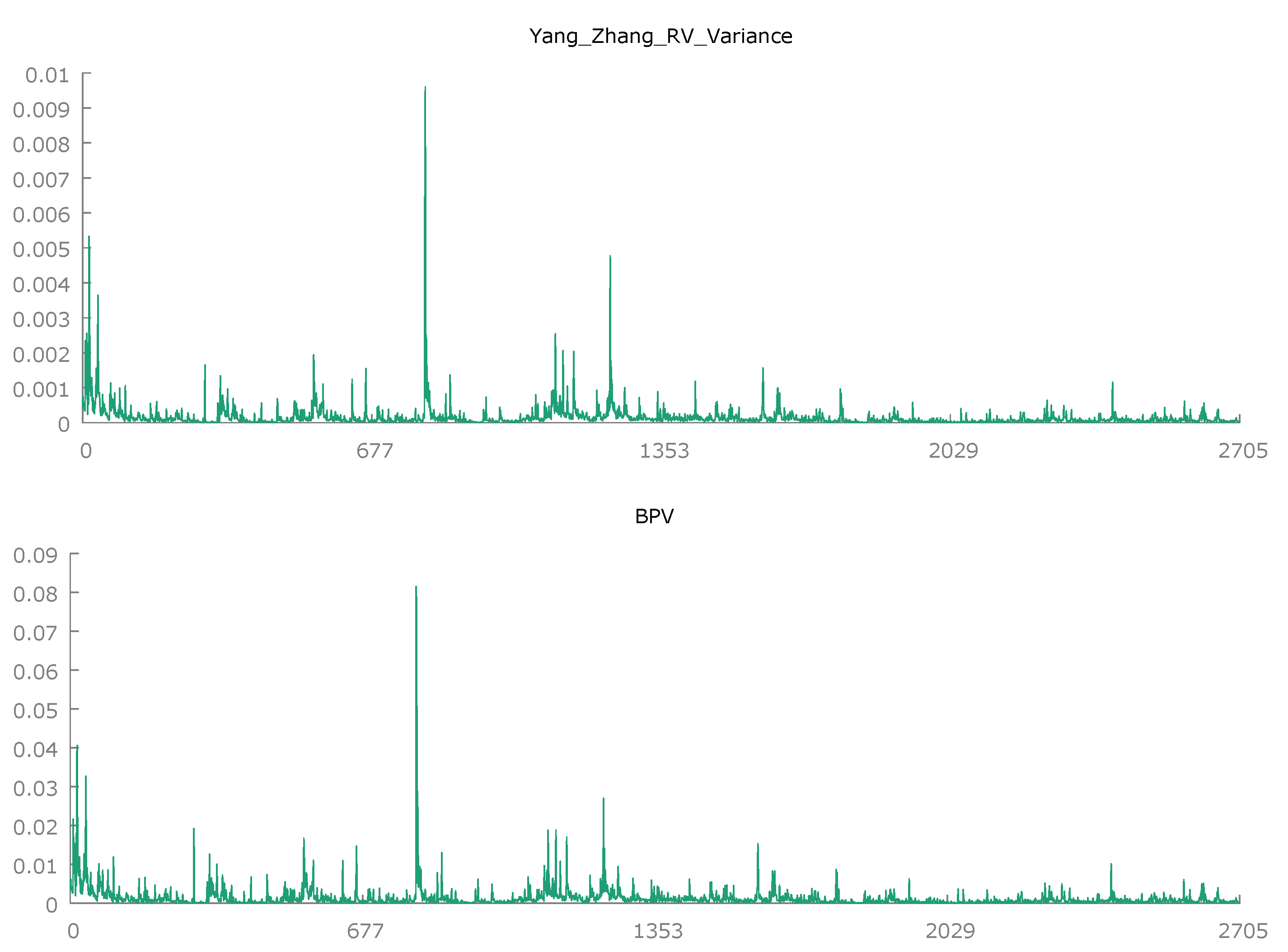

Table 1.
Descriptive statistics daily continuously compounded Bitcoin returns.
| Mean | Median | Minimum | Maximum |
| 0.00076720 | 0.00070766 | -0.50261 | 0.17845 |
| Standard Deviation | Coefficient of Variation | Skewness | Excess Kurtosis |
| 0.035832 | 46.705 | -1.1456 | 17.089 |
Table 2.
Descriptive statistics YZ RV and Barndorff-Nielson and Shephard RV benchmark.
| Yang-Zhang RV | |||
| Mean | Median | Minimum | Maximum |
| 0.00015919 | 7.6161e-05 | 1.1269e-06 | 0.0096028 |
| Standard Deviation | Coefficient of Variation | Skewness | Excess Kurtosis |
| 0.00036679 | 2.3042 | 12.963 | 252.83 |
| Barndorff-Nielson and Shephard RV benchmark | |||
| Mean | Median | Minimum | Maximum |
| 0.0013513 | 0.00062817 | 9.5734e-06 | 0.081530 |
| Standard Deviation | Coefficient of Variation | Skewness | Excess Kurtosis |
| 0.0031696 | 2.3457 | 13.347 | 272.57 |
Table 3.
OLS regression analysis of the benchmark BPV standardised RV estimates on the YZ standardised RV estimates.
Table 3.
OLS regression analysis of the benchmark BPV standardised RV estimates on the YZ standardised RV estimates.
| Coefficient | Standard error | t-ratio | P-value | ||
| Constant | 0.00000 | 0.00392827 | −5.565e-14 | 1.0000 | |
| YZ_RV_Variance | 0.978915 | 0.00392900 | 249.2 | <0.0001*** | |
| Mean dependent variable | 0.000000 | S.D. dependent variable | 1.000000 | ||
| Sum squared residual | 112.8278 | S.E. of regression | 0.204308 | ||
| R-squared | 0.958274 | Adjusted R-squared | 0.958258 | ||
| F (1, 2703) | 62076.36 | P-value (F test) | 0.000000*** | ||
Note: *** indicates significance at the 1% level.
Table 4.
Absolute value of daily Bitcoin returns regressed on 10 lags of itself.
| Coefficient | Standard error | t-ratio | P-value | |
| const | 0.0105661 | 0.00107099 | 9.866 | <0.0001*** |
| absret_1 | 0.0999311 | 0.0193003 | 5.178 | <0.0001*** |
| absret_2 | 0.0318748 | 0.0193945 | 1.643 | 0.1004 |
| absret_3 | 0.0271037 | 0.0193704 | 1.399 | 0.1619 |
| absret_4 | 0.115878 | 0.0193201 | 5.998 | <0.0001*** |
| absret_5 | 0.0665995 | 0.0194122 | 3.431 | 0.0006*** |
| absret_6 | 0.0545868 | 0.0193649 | 2.819 | 0.0049*** |
| absret_7 | 0.0768649 | 0.0192671 | 3.989 | <0.0001*** |
| absret_8 | 0.0465316 | 0.0193108 | 2.410 | 0.0160** |
| absret_9 | 0.0164999 | 0.0192998 | 0.8549 | 0.3927 |
| absret_10 | 0.0154718 | 0.0192085 | 0.8055 | 0.4206 |
| Mean dependent variable | 0.023628 | S.D. dependent variable | 0.026792 | |
| Sum squared residual | 1.789787 | S.E. of regression | 0.025823 | |
| R-squared | 0.074446 | Adjusted R-squared | 0.070997 | |
| F (10, 2684) | 21.58838 | P-value (F) | 3.54e-39 | |
| Log-likelihood | 6035.695 | Akaike criterion | −12049.39 | |
Note: *** and ** indicate significance at the 1% and 5% levels, respectively.
Disclaimer/Publisher’s Note: The statements, opinions and data contained in all publications are solely those of the individual author(s) and contributor(s) and not of MDPI and/or the editor(s). MDPI and/or the editor(s) disclaim responsibility for any injury to people or property resulting from any ideas, methods, instructions or products referred to in the content. |
© 2026 by the authors. Licensee MDPI, Basel, Switzerland. This article is an open access article distributed under the terms and conditions of the Creative Commons Attribution (CC BY) license.
Copyright: This open access article is published under a Creative Commons CC BY 4.0 license, which permit the free download, distribution, and reuse, provided that the author and preprint are cited in any reuse.


